RANDOM GEOMETRIC GRAPH DIAMETER IN THE UNIT
17
RANDOM GEOMETRIC GRAPH DIAMETER IN THE UNIT BALL ROBERT B. ELLIS, JEREMY L. MARTIN, AND CATHERINE YAN Abstract. The unit ball random geometric graph G = G d p (λ, n) has as its vertices n points distributed independently and uniformly in the unit ball in R d , with two vertices adjacent if and only if their ‘p-distance is at most λ. Like its cousin the Erd˝ os-R´ enyi random graph, G has a connectivity threshold : an asymptotic value for λ in terms of n, above which G is connected and below which G is disconnected. In the connected zone, we determine upper and lower bounds for the graph diameter of G. Specifically, almost always, diamp(B)(1 - o(1))/λ ≤ diam(G) ≤ diamp(B)(1 + O((ln ln n/ ln n) 1/d ))/λ, where diamp(B) is the ‘p-diameter of the unit ball B. We employ a combination of methods from probabilistic combinatorics and stochastic geometry. 1. Introduction A random geometric graph consists of a set of vertices distributed randomly over some metric space X , with two vertices joined by an edge if the distance between them is sufficiently small. This construction presents a natural alternative to the classical Erd˝ os-R´ enyi random graph model, in which the presence of each edge is an independent event (see, e.g., [2]). The study of random geometric graphs is a relatively new area; the monograph [9] by M. Penrose is the current authority. In addition to their theoretical interest, random geometric graphs have many applica- tions, including wireless communication networks; see, e.g., [4, 10, 12]. In this article, we study the unit ball random geometric graph G = G d p (λ, n), defined as follows. Let d and n be positive integers, B the Euclidean unit ball in R d centered at the origin, λ a positive real number, and p ∈ [1, ∞] (that is, either p ∈ [1, ∞) or p = ∞). Let V n be a set of n points in B, distributed independently and uniformly with respect to Lebesgue measure on R d . Then G is the graph with vertex set V n , where two vertices x =(x 1 ,...,x d ) and y =(y 1 ,...,y d ) are adjacent if and only if kx - yk p ≤ λ. (Thus the larger λ is, the more edges G has.) Here k·k p is the ‘ p -metric defined by kx - yk p = ( (∑ d i=1 |x i - y i | p ) 1/p for p ∈ [1, ∞), max{|x i - y i | :1 ≤ i ≤ d} for p = ∞, where the case p = 2 gives the standard Euclidean metric on R d . When d = 1, G is known as a random interval graph. (Note that the value of p is immaterial when d = 1.) Random interval graphs have been studied extensively in the literature; the asymptotic distributions for the number of isolated vertices and the number of connected components were determined precisely by E. Godehardt and J. Jaworski [7]. The random Euclidean unit disk graph G 2 2 (λ, n) was studied by X. Jia and the first and third authors [5]. 1 Please note that this is an author-produced PDF of an article accepted for publication following peer review. The publisher version is available on its site. Random geometric graph diameter in the unit ball (with Robert B. Ellis and Catherine Yan) Algorithmica 47, no. 4 (2007), 421--438. The original publication is available at www.springerlink.com: http://dx.doi.org/10.1007/s00453-006-0172-y Open Access version: http://kuscholarworks.ku.edu/dspace/. [This document contains the author's accepted manuscript. For the publisher's version, see the link in the header of this document.]
Transcript of RANDOM GEOMETRIC GRAPH DIAMETER IN THE UNIT
RANDOM GEOMETRIC GRAPH DIAMETER IN THE UNIT
BALL
ROBERT B. ELLIS, JEREMY L. MARTIN, AND CATHERINE YAN
Abstract. The unit ball random geometric graph G = Gdp(λ, n) has as its
vertices n points distributed independently and uniformly in the unit ball inR
d, with two vertices adjacent if and only if their `p-distance is at most λ.Like its cousin the Erdos-Renyi random graph, G has a connectivity threshold :an asymptotic value for λ in terms of n, above which G is connected and belowwhich G is disconnected. In the connected zone, we determine upper and lowerbounds for the graph diameter of G. Specifically, almost always, diamp(B)(1−
o(1))/λ ≤ diam(G) ≤ diamp(B)(1 + O((ln lnn/ ln n)1/d))/λ, where diamp(B)is the `p-diameter of the unit ball B. We employ a combination of methodsfrom probabilistic combinatorics and stochastic geometry.
1. Introduction
A random geometric graph consists of a set of vertices distributed randomly oversome metric space X , with two vertices joined by an edge if the distance betweenthem is sufficiently small. This construction presents a natural alternative to theclassical Erdos-Renyi random graph model, in which the presence of each edge isan independent event (see, e.g., [2]). The study of random geometric graphs is arelatively new area; the monograph [9] by M. Penrose is the current authority. Inaddition to their theoretical interest, random geometric graphs have many applica-tions, including wireless communication networks; see, e.g., [4, 10, 12].
In this article, we study the unit ball random geometric graph G = Gdp(λ, n),
defined as follows. Let d and n be positive integers, B the Euclidean unit ball inR
d centered at the origin, λ a positive real number, and p ∈ [1,∞] (that is, eitherp ∈ [1,∞) or p = ∞). Let Vn be a set of n points in B, distributed independentlyand uniformly with respect to Lebesgue measure on R
d. Then G is the graph withvertex set Vn, where two vertices x = (x1, . . . , xd) and y = (y1, . . . , yd) are adjacentif and only if ‖x − y‖p ≤ λ. (Thus the larger λ is, the more edges G has.) Here‖ · ‖p is the `p-metric defined by
‖x − y‖p =
{
(∑d
i=1 |xi − yi|p)1/p
for p ∈ [1,∞),
max{|xi − yi| : 1 ≤ i ≤ d} for p = ∞,
where the case p = 2 gives the standard Euclidean metric on Rd.
When d = 1, G is known as a random interval graph. (Note that the value of p isimmaterial when d = 1.) Random interval graphs have been studied extensively inthe literature; the asymptotic distributions for the number of isolated vertices andthe number of connected components were determined precisely by E. Godehardtand J. Jaworski [7]. The random Euclidean unit disk graph G2
2(λ, n) was studiedby X. Jia and the first and third authors [5].
1
Ple
ase
note
that
this
is a
n au
thor
-pro
duce
d P
DF
of a
n ar
ticle
acc
epte
d fo
r pub
licat
ion
follo
win
g pe
er re
view
. The
pub
lishe
r ver
sion
is a
vaila
ble
on it
s si
te.
Random geometric graph diameter in the unit ball (with Robert B. Ellis and Catherine Yan) Algorithmica 47, no. 4 (2007), 421--438. The original publication is available at www.springerlink.com: http://dx.doi.org/10.1007/s00453-006-0172-y Open Access version: http://kuscholarworks.ku.edu/dspace/.
[This document contains the author's accepted manuscript. For the publisher's version, see the link in the header of this document.]
2 ROBERT B. ELLIS, JEREMY L. MARTIN, AND CATHERINE YAN
In the present article, we focus on the case d ≥ 2 and p ∈ [1,∞], but also com-ment along the way on the special case d = 1. We are interested in the asymptoticbehavior of the connectivity and graph diameter of G as n → ∞ and λ → 0. In fact,G has a connectivity threshold : roughly speaking, an expression for λ as a func-tion of n, above which G is connected and below which G is disconnected. (Thisbehavior is ubiquitous in the theory of the Erdos-Renyi random graph model; cf.[2].)
We are interested primarily in the combinatorial graph diameter of G, diam(G),above the connectivity threshold. Our results include
• a lower bound for diam(G) (Proposition 7 of §4);• an “absolute” upper bound diam(G) < K/λ, where K is a constant de-
pending only on d (Theorem 8 of §5); and• an asymptotically tight upper bound within a factor of the form (1 + o(1))
of the lower bound, the proof of which builds on the absolute upper bound(Theorem 10 of §6).
2. Definitions and Notation
As mentioned above, the main object of our study is the random geometricgraph G = Gd
p(λ, n), where d ≥ 1 is the dimension of the ambient unit ball B,p ∈ [1,∞] describes the metric, λ > 0 is the `p-distance determining adjacency, andn is the number of vertices. We will generally avoid repeating the constraints onthe parameters.
The graph distance dG(x, y) between two vertices x, y ∈ Vn is defined to be thelength of the shortest path between x and y in G, or ∞ if there is no such path.The graph diameter of G is defined to be diam(G) := max{dG(x, y) : x, y ∈ Vn}.This graph-theoretic quantity is not to be confused with the `p-diameter of a setX ⊆ R
d, defined as diamp(X) := sup{‖x − y‖p : x, y ∈ X}. The `p-ball of radiusr centered at x ∈ R
d is defined as
Bdp(x, r) := {y ∈ R
d : ‖x − y‖p ≤ r},while the `p-ball of radius r around a set X ⊆ R
d is Bdp(X, r) := ∪x∈XBd
p(x, r).
The origin of Rd is O := (0, . . . , 0); when the center of a ball is not explicitly given,
we define Bdp(r) := Bd
p(O, r). Thus B = Bd2 (1). The `p-diameter of B is
diamp(B) =
{
2d1/p−1/2 when 1 ≤ p ≤ 2,
2 when 2 ≤ p ≤ ∞.
The distance dp(X, Y ) between two sets X, Y ⊆ Rd is defined as inf{‖x−y‖p : x ∈
X, y ∈ Y }. The boundary ∂X of X is its closure minus its interior (in the usualtopology on R
d), and its volume vol(X) is its Lebesgue measure.We will make frequent use of the quantity
(1) αdp :=
vol(Bdp(r))
vol(Bd2 (r))
=Γ
(
p+1p
)d
· Γ(
2+d2
)
Γ(
32
)d · Γ(
p+dp
) ,
where Γ is the usual gamma function (see, e.g., [11]). The calculation of αdp, along
with the proofs of several other useful facts about `p-geometry, may be found inthe Appendix at the end of the article.
Random geometric graph diameter in the unit ball (with Robert B. Ellis and Catherine Yan) Algorithmica 47, no. 4 (2007), 421--438. The original publication is available at www.springerlink.com: http://dx.doi.org/10.1007/s00453-006-0172-y Open Access version: http://kuscholarworks.ku.edu/dspace/.
RANDOM GEOMETRIC GRAPH DIAMETER 3
We will say that the random graph G has a property P almost always, or a.a., if
limn→∞
Pr [G has property P ] = 1.
By the notation f(n) = o(g(n)) and f(n) = O(g(n)), we mean, respectively,limn→∞ f(n)/g(n) = 0 and lim supn→∞ f(n)/g(n) ≤ c, for some absolute non-negative constant c.
3. Connectivity thresholds
In order for G = Gdp(λ, n) to have finite diameter, it must be connected. There-
fore, we seek a connectivity threshold – a lower bound on λ so that G is almostalways connected. When d = 1, all `p-metrics are identical. For this case we nowquote parts of Theorems 10 and 12 of [7], to which we refer the reader for their pre-cise determination of the asymptotic Poisson distributions of the number of isolatedvertices and the number of connected components.
Theorem 1 (Godehardt, Jaworski). Let λ1(n) = 1n (log n + c + o(1)) and λ2(n) =
2n (log n + c + o(1)), where c is a constant. Then
limn→∞
Pr[G1p(λ1(n), n)has an isolated vertex ] = e−e−c
,
limn→∞
Pr[G1p(λ2(n), n)is connected ] = e−e−c
.
In particular, by replacing c in Theorem 1 with a nonnegative sequence γ(n) →∞, almost always G1
p(λ1(n), n) has no isolated vertices and G1p(λ2(n), n) is con-
nected. The case d = 1 is exceptional in that the thresholds for having isolatedvertices and for connectivity are separated.
For d ≥ 2, we will use the fact that the connectivity threshold coincides with thethreshold for the disappearance of isolated vertices, which follows from two theoremsof M. Penrose. First we compute the threshold for isolated vertices, which is easierto calculate.
Proposition 2. Let d ≥ 2, let p ∈ [1,∞], and let α = αdp be the constant of (1).
Suppose γ(n) is a nonnegative sequence such that limn→∞ γ(n) → ∞, and that
λ ≥(
1
αn
(
2(d − 1)
dln n +
2
dln ln n + γ(n)
))1/d
.
Then, almost always, G = Gdp(λ, n) has no isolated vertices.
Proof. Let Vn = {v1, v2, . . . , vn} be the vertex set of G. For each vertex vi, let Ai
be the event that vi is an isolated vertex, and let Xi be the indicator of Ai; that is,Xi = 1 if Ai occurs and 0 otherwise. Set X = X1 + X2 + · · · + Xn. We will showthat E[X ] = o(1).
By definition, vi is isolated if and only if there are no other vertices in Bdp(vi, λ)∩
B. We condition Pr[Ai] on the `2-distance from vi to the origin O. If ‖vi − O‖2 ∈[0, 1 − d1/2λ), then Bd
p(vi, λ) ⊆ B. Otherwise, if ‖vi − O‖2 ∈ (1 − d1/2λ, 1], then
the volume of Bdp(vi, λ) ∩ B is not less than 1
2vol(Bdp(vi, λ))(1 + O(λ)). Hence
Pr[Ai] ≤ (1 − d1/2λ)d(1 − αλd)n−1 +
(1 − (1 − d1/2λ)d)
(
1 − αλd
2(1 + O(λ))
)n−1
.
Random geometric graph diameter in the unit ball (with Robert B. Ellis and Catherine Yan) Algorithmica 47, no. 4 (2007), 421--438. The original publication is available at www.springerlink.com: http://dx.doi.org/10.1007/s00453-006-0172-y Open Access version: http://kuscholarworks.ku.edu/dspace/.
4 ROBERT B. ELLIS, JEREMY L. MARTIN, AND CATHERINE YAN
Using 1 − x = e−x(1 + o(1)) as x → 0 and the binomial expansion, we have
Pr[Ai] ≤ (1 + o(1))e−αnλd
+ (dd1/2λ + O(λ2))(1 + o(1))e−αnλd/2.
The first term is o(n−1) for d ≥ 2. By linearity of expectation, E[X ] = n · Pr[Ai],and so
E[X ] ≤ o(1) + d3/2nλ(1 + o(1))n−1+1/d(ln n)−1/de−γ(n)/2 .
The second term is o(1), and so Pr[X > 0] ≤ E[X ] ≤ o(1); that is, almost always,G has no isolated vertices. �
The number of isolated vertices below the threshold is easy to compute in certainspecial cases. For example, if p ∈ [1,∞], d = 2, λ =
√
c ln n/n, and 0 ≤ c < α−1,then a minor modification of [5, Theorem 1] yields X = (1 + o(1))n1−αc almostalways. In general, to determine the behavior of X more exactly would requirecomplicated integrals that describe the volume of Bd
p(vi, λ)∩B near the boundaryof B (cf. [9, Chapter 8]). For our purposes, it suffices to concentrate on the valuesof λ for which G has no isolated vertices.
For d ≥ 2 and p ∈ (1,∞], the connectivity threshold for the unit-cube randomgeometric graph coincides with the threshold for lacking isolated vertices. We quotePenrose’s theorem [8, Thm. 1.1] after some supporting definitions. Define the unit
cube geometric graph H = Hdp (λ, n) analogously to G = Gd
p(λ, n), except that its
vertices are points in [0, 1]d rather than B. For any nonnegative integer k, define
ρ(H ; κ ≥ k + 1) = min{λ | H has vertex connectivity κ ≥ k + 1},(2a)
ρ(H ; δ ≥ k + 1) = min{λ | H has minimum degree δ ≥ k + 1}.(2b)
Theorem 3 (Penrose). Let p ∈ (1,∞] and let k ≥ 0 be an integer. Then
limn→∞
Pr[ ρ(H ; κ ≥ k + 1) = ρ(H ; δ ≥ k + 1) ] = 1.
When k = 0, Theorem 3 asserts that as λ increases (forcing more edges into thegraph), almost always, H becomes connected simultaneously as the last isolatedvertex disappears. In the proof of Theorem 3 in [8], Penrose shows that the limitingprobability distributions for ρ(H ; κ ≥ k +1) and ρ(H ; δ ≥ k +1) are the same. Theproof requires only a series of geometric and probabilistic arguments which hold inthe unit ball as well as in the unit cube (see, in particular, Sections 2 and 5 of [8]),so we have as an immediate corollary the following.
Corollary 4. Let d ≥ 2 and p ∈ (1,∞], and let λ = λ(n) be sufficiently large
so that, almost always, G = Gdp(λ(n), n) has no isolated vertices. Then, almost
always, G is connected.
We now consider the case that d ≥ 2 and p = 1. Here Theorem 3 does notapply. However, we can appeal to two general results about the behavior of arandom geometric graph in an `p-metric space whose boundary is a compact (d−1)-submanifold of R
d For such a graph, Theorem 7.2 of [9] provides a threshold forthe disappearance of isolated vertices, and Theorem 13.7 provides a threshold forconnectivity. Applying these results to G, with the thresholds for G defined as in(2a) and (2b), we obtain the following fact.
Random geometric graph diameter in the unit ball (with Robert B. Ellis and Catherine Yan) Algorithmica 47, no. 4 (2007), 421--438. The original publication is available at www.springerlink.com: http://dx.doi.org/10.1007/s00453-006-0172-y Open Access version: http://kuscholarworks.ku.edu/dspace/.
RANDOM GEOMETRIC GRAPH DIAMETER 5
Proposition 5. Let d ≥ 2, p ∈ [1,∞], and G = Gdp(λ(n), n). Let α = αd
p be the
constant of (1), and let k ≥ 0 be an integer. Then, almost always,
limn→∞
(
nα
log nρ(G; κ ≥ k + 1)d
)
= limn→∞
(
nα
log nρ(G; δ ≥ k + 1)d
)
=2(d − 1)
d.
We now collect the above results to present the connectivity thresholds that wewill use in the rest of the paper.
Theorem 6. Let G = Gdp(λ, n) and let α = αd
p be the constant of (1).
(i) Suppose that d ≥ 2, p ∈ (1,∞], γ(n) is a nonnegative sequence such that
γ(n) → ∞ and
λ ≥(
1
αn
(
2(d − 1)
dln n +
2
dln ln n + γ(n)
))1/d
.
Then, almost always, G is connected.
(ii) Suppose that d ≥ 2, p ∈ [1,∞], and λ = (c ln n/n)1/d for some constant
c > 0. Then, almost always, G is connected if c > (2(d − 1)/(dα)), and
disconnected if c < (2(d − 1)/(dα)).(iii) Suppose that d = 1, p ∈ [1,∞], and λ = 2(ln n + γ(n))/n. Then, almost
always, G is connected if γ(n) → ∞ and disconnected if γ(n) → −∞.
Assertion (i) follows from combining Proposition 2 with Corollary 4, and asser-tion (ii) is implied by Proposition 5. (When p > 1 and d ≥ 2, the lower bound in(ii) is implied by the stronger bound in (i).) Assertion (iii) is implied by Theorem 1and its accompanying remarks.
4. A lower bound for diameter
When G is connected, B will usually contain two vertices whose `p-distance is(asymptotically) diamp(B). Therefore, the diameter of G will almost always be atleast diamp(B)(1 − o(1))/λ. The precise statement is as follows.
Proposition 7 (Diameter lower bound). Let d ≥ 1 and p ∈ [1,∞], and suppose
that λ = λ(n) is sufficiently large so that Theorem 6 guarantees that almost always,
G = Gdp(λ, n) is connected. If h = h(n) satisfies
(3) limn→∞
h(d+1)/2n = ∞,
then, almost always,
diam(G) ≥ 1 − h
λdiamp(B) =
{
2(1− h)d1/p−1/2/λ if p ≤ 2,
2(1− h)/λ if p ≥ 2.
Proof. Let ±a be a pair of antipodes of the unit ball B, chosen as in Figure 4, andlet ±C be the spherical cap formed by slicing B with hyperplanes at distance hfrom ±a respectively, perpendicular to the line joining a and −a. Let A be theevent that at least one of the two caps ±C contains no vertex of Vn. Then
Pr[A] = 2 Pr[C ∩ Vn = ∅] = 2
(
1 − vol(C)
vol(B)
)n
≤ 2 exp
(
−nvol(C)
vol(B)
)
.
On the other hand, vol(C)/vol(B) = O(h(d+1)/2) by (18) of §A.3, which togetherwith the condition (3) on h implies that Pr[A] = o(1). That is, G almost always
Random geometric graph diameter in the unit ball (with Robert B. Ellis and Catherine Yan) Algorithmica 47, no. 4 (2007), 421--438. The original publication is available at www.springerlink.com: http://dx.doi.org/10.1007/s00453-006-0172-y Open Access version: http://kuscholarworks.ku.edu/dspace/.
6 ROBERT B. ELLIS, JEREMY L. MARTIN, AND CATHERINE YAN
contains a vertex in each of C and −C. The result now follows from the definitionof G and the lower bound (19) on the `p-distance between C and −C. �
Note that for all d ≥ 1, h can be chosen to satisfy both (3) and limn→∞ h/λ = 0.Also, if the limit in (3) is a nonnegative constant, then limn→∞ Pr[A] > 0; that is,vertices are not guaranteed in both caps. For the case p = 2, Proposition 7 can bestrengthened by identifying a collection of mutually disjoint antipodal pairs of capsof height h and showing that, almost always, both caps in at least one pair containa vertex. Such a collection corresponds to an antipodally symmetric spherical code(see [3]).
5. The absolute upper bound
In this section we prove that when G is connected, the graph distance dG(x, y)between two vertices x, y ∈ Vn is at most K‖x − y‖p/λ, where K > 0 is a con-stant independent of n and p, but dependent on d. As a consequence, diam(G) ≤Kdiamp(B)/λ. This will not be strong enough to meet (asymptotically) the lowerbound in Proposition 7, but does guarantee a short path between any pair of ver-tices. This fact will be used repeatedly in the proof of the tight upper bound inTheorem 10 of §6. It is sufficient to prove the following Theorem 8, since for anytwo points x, y ∈ R
d, we have ‖x − y‖2 ≤ d1/2‖x − y‖p.
Theorem 8. Let d ≥ 2, and suppose that λ = λ(n) is sufficiently large so that
Theorem 6 guarantees that almost always, G = Gdp(λ, n) is connected. Then for
any two points x, y ∈ Vn there exists a constant K independent of n and p such
that as n → ∞, almost always,
dG(x, y) ≤ K‖x − y‖2
λ.
The proof is based on Proposition 9 below. For any two vertices x, y ∈ Vn, let
Tx,y(k) =[
convex closure of (Bd2 (x, kλ) ∪ Bd
2 (y, kλ))]
∩ B.
Thus Tx,y is a “lozenge”-shaped region. Let An(k) be the event that there exist
two vertices x, y ∈ Vn such that (i) at least one point is inside Bd2(O, 1−(k+
√d)λ),
and (ii) there is no path of G that lies in Tx,y(k) and connects x and y. The proofof our next result uses ingredients from [9, p. 285], adapted and extended for ourpresent purposes.
Proposition 9. Under the same assumptions as in Theorem 8, there exists a
constant k0 > 0, such that for all k > k0,
limn→∞
Pr[An(k)] = 0.
Proof. First, we cover the unit ball B with d-dimensional cubes, each of side lengthελ, where ε = 1/(4d). Let Ld be the set of centers of these cubes, and for eachz ∈ Ld, denote the closed cube centered at z by Qz.
Suppose An(k) occurs for a pair of vertices x, y; without loss of generality, sup-
pose y ∈ Bd2 (O, 1 − (k +
√d)λ). Abbreviate Tx,y(k) by Tx,y.
Step 1. First we construct a connected subset P ⊆ Tx,y such that
(i) Bdp(P, λ/4) ⊆ B;
(ii) diam2(P ) ≥ (k −√
d)λ; and(iii) Bd
p(P, λ/4) ∩ Vn = ∅.
Random geometric graph diameter in the unit ball (with Robert B. Ellis and Catherine Yan) Algorithmica 47, no. 4 (2007), 421--438. The original publication is available at www.springerlink.com: http://dx.doi.org/10.1007/s00453-006-0172-y Open Access version: http://kuscholarworks.ku.edu/dspace/.
RANDOM GEOMETRIC GRAPH DIAMETER 7
y
w
ux
PSfrag replacements
∂B
∂Tx,y
P1
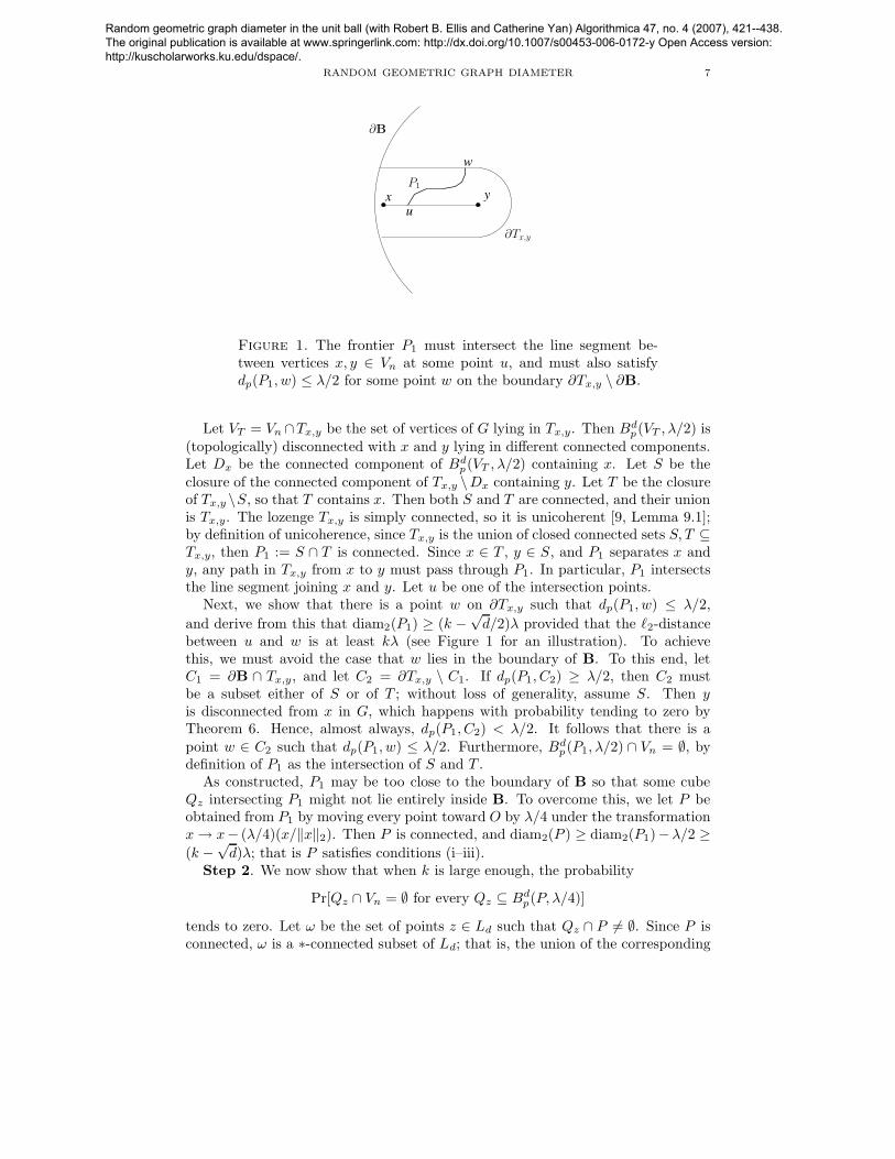
Figure 1. The frontier P1 must intersect the line segment be-tween vertices x, y ∈ Vn at some point u, and must also satisfydp(P1, w) ≤ λ/2 for some point w on the boundary ∂Tx,y \ ∂B.
Let VT = Vn ∩Tx,y be the set of vertices of G lying in Tx,y. Then Bdp(VT , λ/2) is
(topologically) disconnected with x and y lying in different connected components.Let Dx be the connected component of Bd
p(VT , λ/2) containing x. Let S be theclosure of the connected component of Tx,y \Dx containing y. Let T be the closureof Tx,y \S, so that T contains x. Then both S and T are connected, and their unionis Tx,y. The lozenge Tx,y is simply connected, so it is unicoherent [9, Lemma 9.1];by definition of unicoherence, since Tx,y is the union of closed connected sets S, T ⊆Tx,y, then P1 := S ∩ T is connected. Since x ∈ T , y ∈ S, and P1 separates x andy, any path in Tx,y from x to y must pass through P1. In particular, P1 intersectsthe line segment joining x and y. Let u be one of the intersection points.
Next, we show that there is a point w on ∂Tx,y such that dp(P1, w) ≤ λ/2,
and derive from this that diam2(P1) ≥ (k −√
d/2)λ provided that the `2-distancebetween u and w is at least kλ (see Figure 1 for an illustration). To achievethis, we must avoid the case that w lies in the boundary of B. To this end, letC1 = ∂B ∩ Tx,y, and let C2 = ∂Tx,y \ C1. If dp(P1, C2) ≥ λ/2, then C2 mustbe a subset either of S or of T ; without loss of generality, assume S. Then yis disconnected from x in G, which happens with probability tending to zero byTheorem 6. Hence, almost always, dp(P1, C2) < λ/2. It follows that there is apoint w ∈ C2 such that dp(P1, w) ≤ λ/2. Furthermore, Bd
p(P1, λ/2) ∩ Vn = ∅, bydefinition of P1 as the intersection of S and T .
As constructed, P1 may be too close to the boundary of B so that some cubeQz intersecting P1 might not lie entirely inside B. To overcome this, we let P beobtained from P1 by moving every point toward O by λ/4 under the transformationx → x− (λ/4)(x/‖x‖2). Then P is connected, and diam2(P ) ≥ diam2(P1)−λ/2 ≥(k −
√d)λ; that is P satisfies conditions (i–iii).
Step 2. We now show that when k is large enough, the probability
Pr[Qz ∩ Vn = ∅ for every Qz ⊆ Bdp(P, λ/4)]
tends to zero. Let ω be the set of points z ∈ Ld such that Qz ∩ P 6= ∅. Since P isconnected, ω is a ∗-connected subset of Ld; that is, the union of the corresponding
Random geometric graph diameter in the unit ball (with Robert B. Ellis and Catherine Yan) Algorithmica 47, no. 4 (2007), 421--438. The original publication is available at www.springerlink.com: http://dx.doi.org/10.1007/s00453-006-0172-y Open Access version: http://kuscholarworks.ku.edu/dspace/.
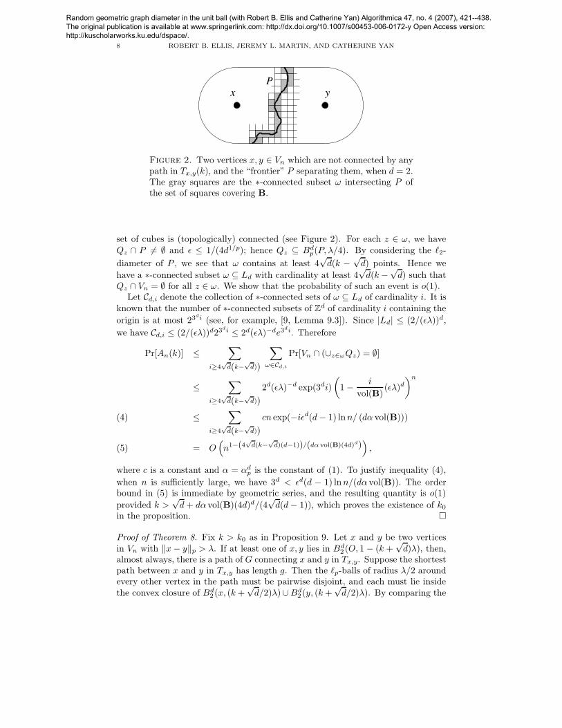
8 ROBERT B. ELLIS, JEREMY L. MARTIN, AND CATHERINE YAN
Pyx
Figure 2. Two vertices x, y ∈ Vn which are not connected by anypath in Tx,y(k), and the “frontier” P separating them, when d = 2.The gray squares are the ∗-connected subset ω intersecting P ofthe set of squares covering B.
set of cubes is (topologically) connected (see Figure 2). For each z ∈ ω, we haveQz ∩ P 6= ∅ and ε ≤ 1/(4d1/p); hence Qz ⊆ Bd
p(P, λ/4). By considering the `2-
diameter of P , we see that ω contains at least 4√
d(k −√
d) points. Hence we
have a ∗-connected subset ω ⊆ Ld with cardinality at least 4√
d(k −√
d) such thatQz ∩ Vn = ∅ for all z ∈ ω. We show that the probability of such an event is o(1).
Let Cd,i denote the collection of ∗-connected sets of ω ⊆ Ld of cardinality i. It isknown that the number of ∗-connected subsets of Z
d of cardinality i containing the
origin is at most 23di (see, for example, [9, Lemma 9.3]). Since |Ld| ≤ (2/(ελ))d,
we have Cd,i ≤ (2/(ελ))d23di ≤ 2d(ελ)−de3di. Therefore
Pr[An(k)] ≤∑
i≥4√
d(k−√
d))
∑
ω∈Cd,i
Pr[Vn ∩ (∪z∈ωQz) = ∅]
≤∑
i≥4√
d(k−√
d))
2d(ελ)−d exp(3di)
(
1 − i
vol(B)(ελ)d
)n
≤∑
i≥4√
d(k−√
d))
cn exp(−iεd(d − 1) ln n/ (dα vol(B)))(4)
= O(
n1−(4√
d(k−√
d)(d−1))/(dα vol(B)(4d)d))
,(5)
where c is a constant and α = αdp is the constant of (1). To justify inequality (4),
when n is sufficiently large, we have 3d < εd(d − 1) ln n/(dα vol(B)). The orderbound in (5) is immediate by geometric series, and the resulting quantity is o(1)
provided k >√
d + dα vol(B)(4d)d/(4√
d(d − 1)), which proves the existence of k0
in the proposition. �
Proof of Theorem 8. Fix k > k0 as in Proposition 9. Let x and y be two verticesin Vn with ‖x − y‖p > λ. If at least one of x, y lies in Bd
2 (O, 1 − (k +√
d)λ), then,almost always, there is a path of G connecting x and y in Tx,y. Suppose the shortestpath between x and y in Tx,y has length g. Then the `p-balls of radius λ/2 aroundevery other vertex in the path must be pairwise disjoint, and each must lie insidethe convex closure of Bd
2 (x, (k +√
d/2)λ)∪Bd2 (y, (k +
√d/2)λ). By comparing the
Random geometric graph diameter in the unit ball (with Robert B. Ellis and Catherine Yan) Algorithmica 47, no. 4 (2007), 421--438. The original publication is available at www.springerlink.com: http://dx.doi.org/10.1007/s00453-006-0172-y Open Access version: http://kuscholarworks.ku.edu/dspace/.
RANDOM GEOMETRIC GRAPH DIAMETER 9
volume of the `p-balls of radius λ/2 to the volume of Tx,y, we obtain⌊g
2
⌋
vol(
Bdp(x, λ/2)
)
≤ vol(
Bd2 (x, (k +
√d/2)λ)
)
+d2(x, y) · vol(
Bd−12 (x, (k +
√d/2)λ)
)
,
which implies that g ≤ K1 + K2d2(x, y)/λ ≤ (K1
√d + K2)d2(x, y)/λ, where K1
and K2 are constants independent of n and p.If both x and y lie outside Bd
2 (O, 1 − (k +√
d)λ), then we can travel from x to
an intermediate vertex x1 just inside B(O, 1 − (k +√
d)λ) via a path of bounded
length, and then on to y. To this end, let r = max{(αdp)
1/d√
d,√
d}, and let En(k)
be the event that there is a vertex z ∈ Vn such that z 6∈ B(O, 1 − (k +√
d)λ) and
Vn ∩ (B(O, 1 − (k +√
d)λ) ∩ B(z, (k +√
d + 2r)λ)) = ∅. Then
Pr[En(k)] ≤ n(
1 − (1 − (k +√
d)λ)d)
(1 − (√
dλ)d)n = o(1).
Applying this observation with z = x, we can find a point x1 ∈ Vn inside B(O, 1 −(k +
√d)λ) ∩B(x, (k +
√d + 2r)λ). By the preceding argument we can first travel
from x to x1 in Kd2(x, x1)/λ steps, and then from x1 to y in Kd2(x1, y)/λ steps.The total length of the path is no more than K(d2(x, y) + 2d2(x, x1))/λ. Theorem
8 follows from the fact that d2(x, x1) ≤ (k +√
d + 2r)λ. �
We briefly discuss the case that d = 1, so that B is the interval [−1, 1] ⊂ R.Suppose that λ = λ(n) is sufficiently large so that Theorem 6 guarantees that,almost always, G1
p(λ, n) is connected. For any two vertices x, y, the shortest pathbetween them clearly consists of a strictly increasing set of vertices x = x0 < x1 <x2 < · · · < xdG(x,y) = y. Moreover, the balls B(x0, λ/2), B(x2, λ/2), B(x4, λ/2), . . .must be pairwise disjoint (else some xi is redundant). Hence |x−y| ≥ ddG(x, y)/2eλ,and from this it is not hard to deduce that dG(x, y) ≤ 2|x − y|/λ.
6. The asymptotically tight upper bound
In this section, we improve the upper bound in Theorem 8, reducing the constantK to diamp(B) (asymptotically). Our main result is as follows:
Theorem 10. Let d ≥ 2 and p ∈ [1,∞], and suppose that λ = λ(n) is sufficiently
large so that Theorem 6 guarantees that almost always, G = Gdp(λ, n) is connected.
Then as n → ∞, almost always,
diam(G) ≤{
(
2d1/p−1/2 + O(
(ln ln n/ ln n)1/d))
/λ when 1 ≤ p ≤ 2,(
2 + O(
(ln ln n/ lnn)1/d))
/λ when 2 ≤ p ≤ ∞.
That is, almost always, diam(G) ≤ diamp(B)(1 + O((ln ln n/ lnn)1/d))/λ.
The proof uses the geometric ingredients of pins and pincushions. A pin consistsof a collection of evenly spaced, overlapping `p-balls whose centers lie on a diameterof the Euclidean unit d-ball B. By making suitable choices for the geometry, wecan ensure that each intersection of consecutive balls contains a vertex in Vn, sothat the pin provides a “highway” through G. Having done this, we construct apincushion so that every point of B is reasonably close to an `p-ball in one of itsconstituent pins. The following definitions are illustrated in Figure 3.
Random geometric graph diameter in the unit ball (with Robert B. Ellis and Catherine Yan) Algorithmica 47, no. 4 (2007), 421--438. The original publication is available at www.springerlink.com: http://dx.doi.org/10.1007/s00453-006-0172-y Open Access version: http://kuscholarworks.ku.edu/dspace/.
10 ROBERT B. ELLIS, JEREMY L. MARTIN, AND CATHERINE YAN
������������������������������
������������������������������
������������������������������������������
������������������������������������������
������������������������������
������������������������������
������������������������������
�������������������������
������������������
������������
������������������������������
������������������������������
� � � � � � � � � � � �
������������������������������
������������������������������������������
������������������������������������������
������������������������������
������������������������������
������������������������������������������
������������������������������������������
������������������������������
������������������������������
������������������������������
������������������������������������������������������������
������������������������������������������������������������������������
������������������������������������������������������������������������������������
������������������������������������������
������������������������������
� � � � � � � � � � � � !�!�!!�!�!!�!�!!�!�!!�!�!!�!�!
"�"�""�"�""�"�""�"�""�"�""�"�"#�#�#�##�#�#�##�#�#�##�#�#�##�#�#�##�#�#�#
$�$�$�$$�$�$�$$�$�$�$$�$�$�$$�$�$�$$�$�$�$%�%�%�%%�%�%�%%�%�%�%%�%�%�%%�%�%�%%�%�%�%
&�&�&�&&�&�&�&&�&�&�&&�&�&�&&�&�&�&&�&�&�&
'�'�''�'�''�'�''�'�''�'�''�'�'
(�(�((�(�((�(�((�(�((�(�((�(�(
)�)�))�)�))�)�))�)�))�)�))�)�)
*�*�**�*�**�*�**�*�**�*�*+�+�+�++�+�+�++�+�+�++�+�+�++�+�+�++�+�+�+
,�,�,,�,�,,�,�,,�,�,,�,�,
-�-�--�-�--�-�--�-�--�-�--�-�-
.�.�..�.�..�.�..�.�..�.�..�.�.
/�/�/�//�/�/�//�/�/�//�/�/�//�/�/�//�/�/�/
0�0�0�00�0�0�00�0�0�00�0�0�00�0�0�00�0�0�0
1�1�11�1�11�1�11�1�11�1�11�1�1
2�2�22�2�22�2�22�2�22�2�22�2�2
3�3�3�33�3�3�33�3�3�33�3�3�33�3�3�33�3�3�3
4�4�4�44�4�4�44�4�4�44�4�4�44�4�4�4
5�5�55�5�55�5�55�5�55�5�55�5�5
6�6�66�6�66�6�66�6�66�6�66�6�6
7�7�77�7�77�7�77�7�77�7�77�7�7
8�8�88�8�88�8�88�8�88�8�88�8�8
9�9�9�99�9�9�99�9�9�99�9�9�99�9�9�99�9�9�9
:�:�::�:�::�:�::�:�::�:�::�:�:
;�;�;;�;�;;�;�;;�;�;;�;�;;�;�;
<�<�<<�<�<<�<�<<�<�<<�<�<<�<�<
=�=�==�=�==�=�==�=�==�=�==�=�=
>�>�>>�>�>>�>�>>�>�>>�>�>>�>�>
?�?�?�??�?�?�??�?�?�??�?�?�??�?�?�??�?�?�?
@�@�@�@@�@�@�@@�@�@�@@�@�@�@@�@�@�@@�@�@�@
A�A�AA�A�AA�A�AA�A�AA�A�AA�A�A
B�B�BB�B�BB�B�BB�B�BB�B�BB�B�B
C�C�CC�C�CC�C�CC�C�CC�C�CC�C�C
D�D�DD�D�DD�D�DD�D�DD�D�D
E�E�EE�E�EE�E�EE�E�EE�E�EE�E�E
F�F�FF�F�FF�F�FF�F�FF�F�F
G�G�G�GG�G�G�GG�G�G�GG�G�G�GG�G�G�GG�G�G�G
H�H�H�HH�H�H�HH�H�H�HH�H�H�HH�H�H�HH�H�H�H
I�I�I�II�I�I�II�I�I�II�I�I�II�I�I�II�I�I�I
J�J�J�JJ�J�J�JJ�J�J�JJ�J�J�JJ�J�J�JJ�J�J�J
K�K�KK�K�KK�K�KK�K�KK�K�KK�K�K
L�L�LL�L�LL�L�LL�L�LL�L�LL�L�L
M�M�MM�M�MM�M�MM�M�MM�M�MM�M�M
N�N�NN�N�NN�N�NN�N�NN�N�NN�N�N
O�O�O�OO�O�O�OO�O�O�OO�O�O�OO�O�O�OO�O�O�O
P�P�P�PP�P�P�PP�P�P�PP�P�P�PP�P�P�PP�P�P�P
Q�Q�Q�QQ�Q�Q�QQ�Q�Q�QQ�Q�Q�QQ�Q�Q�QQ�Q�Q�Q
R�R�R�RR�R�R�RR�R�R�RR�R�R�RR�R�R�RR�R�R�R
S�S�SS�S�SS�S�SS�S�SS�S�SS�S�S
T�T�TT�T�TT�T�TT�T�TT�T�TT�T�T
U�U�UU�U�UU�U�UU�U�UU�U�UU�U�U
V�V�VV�V�VV�V�VV�V�VV�V�VV�V�V
W�W�W�WW�W�W�WW�W�W�WW�W�W�WW�W�W�WW�W�W�W
X�X�XX�X�XX�X�XX�X�XX�X�XX�X�X
Y�Y�Y�YY�Y�Y�YY�Y�Y�YY�Y�Y�YY�Y�Y�Y
Z�Z�ZZ�Z�ZZ�Z�ZZ�Z�ZZ�Z�Z
[�[�[[�[�[[�[�[[�[�[[�[�[
\�\�\\�\�\\�\�\\�\�\\�\�\
]�]�]�]]�]�]�]]�]�]�]]�]�]�]]�]�]�]
^�^�^^�^�^^�^�^^�^�^^�^�^
_�_�_�__�_�_�__�_�_�__�_�_�__�_�_�_
`�`�`�``�`�`�``�`�`�``�`�`�``�`�`�`
a�a�aa�a�aa�a�aa�a�aa�a�a
b�b�bb�b�bb�b�bb�b�bb�b�b
c�c�cc�c�cc�c�cc�c�cc�c�c
d�d�dd�d�dd�d�dd�d�dd�d�d
e�e�e�ee�e�e�ee�e�e�ee�e�e�ee�e�e�e
f�f�ff�f�ff�f�ff�f�ff�f�f
g�g�g�gg�g�g�gg�g�g�gg�g�g�gg�g�g�g
h�h�h�hh�h�h�hh�h�h�hh�h�h�hh�h�h�h
i�i�ii�i�ii�i�ii�i�ii�i�i
j�j�jj�j�jj�j�jj�j�jj�j�j
k�k�k�kk�k�k�kk�k�k�kk�k�k�kk�k�k�k
l�l�l�ll�l�l�ll�l�l�ll�l�l�ll�l�l�l
m�m�m�mm�m�m�mm�m�m�mm�m�m�mm�m�m�m
n�n�nn�n�nn�n�nn�n�nn�n�n
o�o�oo�o�oo�o�oo�o�oo�o�o
p�p�pp�p�pp�p�pp�p�pp�p�p
q�q�q�qq�q�q�qq�q�q�qq�q�q�qq�q�q�q
r�r�rr�r�rr�r�rr�r�rr�r�r
s�s�s�ss�s�s�ss�s�s�ss�s�s�ss�s�s�s
t�t�tt�t�tt�t�tt�t�tt�t�t
u�u�uu�u�uu�u�uu�u�uu�u�u
v�v�vv�v�vv�v�vv�v�vv�v�v
w�w�w�ww�w�w�ww�w�w�ww�w�w�ww�w�w�w
x�x�x�xx�x�x�xx�x�x�xx�x�x�xx�x�x�x
y�y�y�yy�y�y�yy�y�y�yy�y�y�yy�y�y�y
z�z�z�zz�z�z�zz�z�z�zz�z�z�zz�z�z�z{�{�{{�{�{{�{�{{�{�{{�{�{
|�|�||�|�||�|�||�|�||�|�|}�}�}�}}�}�}�}}�}�}�}}�}�}�}}�}�}�}
~�~�~�~~�~�~�~~�~�~�~~�~�~�~~�~�~�~
�����������������������������������
������������������������������������������������������������
������������������������������������������������������������
�����������������������������������
������������������������������
������������������������������
������������������������������
������������������������������
������������������������������
������������������������������
������������������������������
������������������������������
������������������������������
������������������������������
������������������������������
������������������������������
������������������������������
������������������������������
������������������������������
�������������������������
������������������������������
������������������������������
������������������������������
������������������������������
������������������������������
������������������������������
u1 O
Ou0
r
B
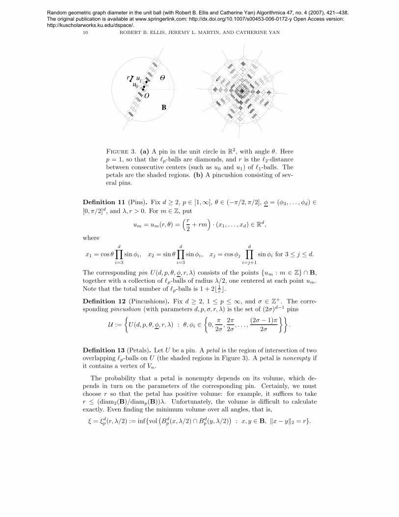
Figure 3. (a) A pin in the unit circle in R2, with angle θ. Here
p = 1, so that the `p-balls are diamonds, and r is the `2-distancebetween consecutive centers (such as u0 and u1) of `1-balls. Thepetals are the shaded regions. (b) A pincushion consisting of sev-eral pins.
Definition 11 (Pins). Fix d ≥ 2, p ∈ [1,∞], θ ∈ (−π/2, π/2], φ = (φ3, . . . , φd) ∈[0, π/2]d, and λ, r > 0. For m ∈ Z, put
um = um(r, θ) =(r
2+ rm
)
· (x1, . . . , xd) ∈ Rd,
where
x1 = cos θ
d∏
i=3
sin φi, x2 = sin θ
d∏
i=3
sinφi, xj = cosφj
d∏
i=j+1
sin φi for 3 ≤ j ≤ d.
The corresponding pin U(d, p, θ, φ, r, λ) consists of the points {um : m ∈ Z} ∩ B,together with a collection of `p-balls of radius λ/2, one centered at each point um.Note that the total number of `p-balls is 1 + 2b 1
r c.Definition 12 (Pincushions). Fix d ≥ 2, 1 ≤ p ≤ ∞, and σ ∈ Z
+. The corre-sponding pincushion (with parameters d, p, σ, r, λ) is the set of (2σ)d−1 pins
U :=
{
U(d, p, θ, φ, r, λ) : θ, φi ∈{
0,π
2σ,2π
2σ, . . . ,
(2σ − 1)π
2σ
}}
.
Definition 13 (Petals). Let U be a pin. A petal is the region of intersection of twooverlapping `p-balls on U (the shaded regions in Figure 3). A petal is nonempty ifit contains a vertex of Vn.
The probability that a petal is nonempty depends on its volume, which de-pends in turn on the parameters of the corresponding pin. Certainly, we mustchoose r so that the petal has positive volume: for example, it suffices to taker ≤ (diam2(B)/diamp(B))λ. Unfortunately, the volume is difficult to calculateexactly. Even finding the minimum volume over all angles, that is,
ξ = ξdp(r, λ/2) := inf{vol
(
Bdp(x, λ/2) ∩ Bd
p(y, λ/2))
: x, y ∈ B, ‖x − y‖2 = r}.
Random geometric graph diameter in the unit ball (with Robert B. Ellis and Catherine Yan) Algorithmica 47, no. 4 (2007), 421--438. The original publication is available at www.springerlink.com: http://dx.doi.org/10.1007/s00453-006-0172-y Open Access version: http://kuscholarworks.ku.edu/dspace/.
RANDOM GEOMETRIC GRAPH DIAMETER 11
requires integrals that are not easily evaluated (although for fixed d and r, it iscertainly true that ξ = Θ(λd)). The easiest way to find a lower bound for ξ is toinscribe another `p-ball in the petal.
Lemma 14. Let d ≥ 1, p ∈ [1,∞], λ > 0 and 0 ≤ r ≤ (diamp(B)/diam2(B))λ.
Then, for all x, y ∈ B with ‖x − y‖2 = r,
Bd2
(
x+y2 , r′
)
⊆ Bdp(x, λ/2) ∩ Bd
p(y, λ/2),
where
r′ =
{
λ2 d1/2−1/p − r
2 when 1 ≤ p ≤ 2,λ2 − r
2 when 2 ≤ p ≤ ∞.
In particular,
ξ
vol(B)≥
{
(
λ2 d1/2−1/p − r
2
)dwhen 1 ≤ p ≤ 2,
(
λ2 − r
2
)dwhen 2 ≤ p ≤ ∞.
Proof. Let z ∈ Bd2 (x+y
2 , r′). By the triangle inequality,
‖z − x‖2 ≤∥
∥z − x+y2
∥
∥
2+
∥
∥
x+y2 − x
∥
∥
2≤ r′ + r
2 ,
which, together with (17), implies that ‖z − x‖p ≤ λ/2. That is, z ∈ Bdp(x, λ/2).
The same argument implies that z ∈ Bdp(y, λ/2). The bound on ξ is then a simple
application of (14). �
For the remainder of this section, we work with the pincushion U defined by
(6a) σ = σ(n) = b(ln n)1/dcand
(6b) r = r(n) =
{
λd1/2−1/p(1 − ρ(n)) when 1 ≤ p ≤ 2,
λ(1 − ρ(n)) when 2 ≤ p ≤ ∞,
where
(6c) ρ = ρ(n) =
{
2d1/p−1/2(ln ln n/ ln n)1/d when 1 ≤ p ≤ 2,
2(ln ln n/ lnn)1/d when 2 ≤ p ≤ ∞.
Let τU = τU (n) be the number of empty petals along the pin U ∈ U , and define
τ = τ(n) = max{τU (n) : U ∈ U}.We first calculate an upper bound on τ .
Lemma 15. With the assumptions of Theorem 10, and the parameters σ, r, ρ as
just defined, almost always,
τ ≤ σ(d−1)/2 2
rexp
( −nξ
vol(B)
)
.
Proof. Denote the right-hand side of the desired inequality by T . By linearity ofexpectation,
Pr[τ ≥ T ] ≤ E[|{U : τU ≥ T}|]≤ (2σ)d−1 · Pr[τU∗ ≥ T ],(7)
Random geometric graph diameter in the unit ball (with Robert B. Ellis and Catherine Yan) Algorithmica 47, no. 4 (2007), 421--438. The original publication is available at www.springerlink.com: http://dx.doi.org/10.1007/s00453-006-0172-y Open Access version: http://kuscholarworks.ku.edu/dspace/.
12 ROBERT B. ELLIS, JEREMY L. MARTIN, AND CATHERINE YAN
where U∗ is chosen so as to maximize Pr[τU ≥ T ]. Let Xi be the indicator randomvariable of the event that the ith petal of U ∗ is empty, and let X =
∑
i Xi. NowU∗ contains at most 2/r petals, so by linearity of expectation,
(8) E[X ] ≤ 2
r
(
1 − ξ
vol(B)
)n
≤ 2
rexp
( −nξ
vol(B)
)
.
Also,
var[X ] ≤ E[X ] +∑
i6=j
cov(Xi, Xj),(9)
where the covariance cov(Xi, Xj) for i 6= j is
cov(Xi, Xj) = Pr[XiXj = 1] − Pr[Xi = 1] · Pr[Xj = 1]
=
(
1 − 2ξ
vol(B)
)n
−(
1 − ξ
vol(B)
)2n
≤ o(1) · exp
( −2nξ
vol(B)
)
.(10)
Combining (8), (9) and (10) gives
(11) var[X ] ≤ 2
rexp
( −nξ
vol(B)
)
+4
r2o(1) · exp
( −2nξ
vol(B)
)
.
By Chebyshev’s inequality (cf. [1]) and the bounds for E[X ] and var[X ] in (8) and(11),
Pr[
X ≥ T]
≤ Pr[
|X − E[X ]| ≥ T − E[X ]]
≤ var[X ]
(T − E[X ])2= o
(
1
σd−1
)
.
Now Pr[τU ≥ T ] = Pr[X ≥ T ]. Therefore, substituting this last bound into (7)gives Pr[τ ≥ T ] = o(1), which implies the desired result. �
We can now prove the main result of this section.
Proof of Theorem 10. Let x, y ∈ Vn. We will find vertices x1 and y1 near x and yrespectively, belonging to petals of the pincushion U . From each of x1, y1, we walkalong the appropriate pin to points x2, y2 near the origin and belonging to petals onthe same pin as x1 and y1, respectively. We will then use Theorem 8 to construct apath from x2 to y2, as well as any “detours” needed in case there are missing edgesin the paths along the pins. Without loss of generality, we may assume that
(12) ‖x‖2, ‖y‖2 ≥ (τ + 3/2)r.
The justification for this is deferred until the end of the proof.Let Rx be the (possibly empty) petal nearest to x, and let Ux be the pin contain-
ing Rx. When n is sufficiently large, the distance from x to Rx is at most dπ/2σ.By definition of τ , there is another vertex x1 ∈ Vn, which also lies in a petal onUx, but is closer to the origin, so that ‖x− x1‖2 ≤ dπ/2σ + r(τ + 1). Repeat theseconstructions for y to obtain an analogous vertex y1. Then
‖x − x1‖2, ‖y − y1‖2 ≤ dπ
2σ+ r(τ + 1),
Random geometric graph diameter in the unit ball (with Robert B. Ellis and Catherine Yan) Algorithmica 47, no. 4 (2007), 421--438. The original publication is available at www.springerlink.com: http://dx.doi.org/10.1007/s00453-006-0172-y Open Access version: http://kuscholarworks.ku.edu/dspace/.
RANDOM GEOMETRIC GRAPH DIAMETER 13
and, by Theorem 8,
dG(x, x1), dG(y, y1) ≤(
dπ
2σ+ r(τ + 1)
)
K
λ.
By definition of τ , there is a vertex x2 that belongs to a petal Rx2on Ux (indeed,
lying on the same side of O along Ux) with Rx2⊆ Bd
2 (O, r(τ + 3/2)). In the worstcase, all empty petals in Ux occur non-consecutively between x1 and x2, so for nlarge enough, we have
dG(x1, x2) ≤ ‖x1‖2
r+
2Krτ
λ
≤ ‖x‖2
r+
dπ
2σr+
2Krτ
λ.
The same construction goes through if we replace the x’s with y’s. Moreover,‖x2 − y2‖2 ≤ (2τ + 3)r, so the shortest path in G between x2 and y2 satisfies
dG(x2, y2) ≤(2τ + 3)rK
λ.
Concatenating all the above paths, we find that
dG(x, y) ≤ dG(x, x1) + dG(x1, x2) + dG(x2, y2) + dG(y2, y1) + dG(y1, y)
≤ ‖x‖2 + ‖y‖2
r+
(
dπ
σ+ (8τ + 5)r
)
K
λ+
dπ
σr
≤ diamp(B)
diam2(B)
‖x‖2 + ‖y‖2 + O(ρ)
λ+ O(τ) + O
(
(ln n)−1/d
λ
)
.(13)
By the definitions of r and ρ given in (6b) and (6c), and the bounds on ξ and τ(Lemmas 14 and 15), it follows that
ξ
vol(B)≥ λd ln ln n
ln n≥ ln ln n
n,
where the second inequality follows from the assumption that λ is above the thresh-old for connectivity in Theorem 6. Therefore
τ ≤ 2σ(d−1)/2
rexp
( −nξ
vol(B)
)
≤ 4
λ(ln n)(d−1)/(2d)(ln n)−1 =
O(
(ln n)−(d+1)/(2d))
λ=
o(ρ)
λ.
Plugging this bound for τ into (13) gives
dG(x, y) ≤ diamp(B)
diam2(B)
‖x‖2 + ‖y‖2 + O(ρ)
λ,
and the theorem follows.We now explain the assumption (12). If ‖x‖2, ‖y‖2 ≤ (τ + 3/2)r, then by
Theorem 8, dG(u, v) ≤ (2τ + 3)rK/λ = o(ρ)/λ. On the other hand, if ‖x‖2 ≤(τ +3/2)r ≤ ‖y‖2, then, almost always, there is a vertex x2 ∈ Bd
2 (O, (τ +3/2)r) be-longing to some petal. By the preceding argument, dG(x, y) ≤ o(ρ/λ)+dG(x2, y) ≤(diamp(B)/diam2(B))(‖y‖2 + O(ρ))/λ. �
Random geometric graph diameter in the unit ball (with Robert B. Ellis and Catherine Yan) Algorithmica 47, no. 4 (2007), 421--438. The original publication is available at www.springerlink.com: http://dx.doi.org/10.1007/s00453-006-0172-y Open Access version: http://kuscholarworks.ku.edu/dspace/.
14 ROBERT B. ELLIS, JEREMY L. MARTIN, AND CATHERINE YAN
We conclude with two remarks. First, the proof of Theorem 10 can easilybe adapted to the case d = 1 to obtain the upper bound diam(G1
p(λ, n)) ≤(2 + O(ln ln n/ lnn)) /λ. (Note that when d = 1 a pincushion consists of just onepin.) Second, the technique of Theorem 10 can be extended to obtain the strongerresult dG(x, y) ≤
(
‖x − y‖p + O(
(ln ln n/ lnn)1/d))
/λ, so that the graph distance
approximates the `p-metric. Each pin is replaced by σd−1 evenly spaced parallelpins. We can still bound τ by o(ρ)/λ, but now any two vertices x and y are closeto the same pin, on which a short path from x to y is found. We refer the readerto [6] for details.
Acknowledgements
The authors thank Thomas Schlumprecht, Joel Spencer and Dennis Stanton forvarious helpful discussions and comments. We also thank the anonymous refereesfor several helpful suggestions.
Appendix A. Facts about `p- and spherical geometry
In the body of the article, we used various facts about the Euclidean and `p-geometry of balls and spherical caps. None of these facts are difficult; however, forconvenience we present them together here along with brief proofs.
A.1. Volume of the `p-unit ball. Fix p ∈ [1,∞] and an integer d ≥ 1. Let Bdp(r)
be the `p-ball centered at the origin in Rd with radius r:
Bdp(r) =
{
x ∈ Rd :
d∑
i=1
|xi|p ≤ rp
}
.
We will show that the (d-dimensional) volume of Bdp(r) is
(14) vol(Bdp(r)) =
(2r)dΓ(
p+1p
)d
Γ(
p+dp
) ,
where Γ is the usual gamma function [11]. For d = 1 this is trivial. For d > 1 wehave
vol(Bdp(r)) = 2
∫ r
0
vol(
Bd−1p ((rp − xp)1/p)
)
dx.
Make the substitution u = xp/rp, x = ru1/p, dx = (r/p)u(1−p)/p du. By inductionon d, we obtain
vol(Bdp(r)) =
2drdΓ(
p+1p
)d−1
pΓ(
p+d−1p
)
∫ 1
0
(1 − u)d−1
p u1−p
p du.
Evaluating this integral as in [11, §12.4] yields the desired formula (14). It followsthat
(15) αdp :=
vol(Bdp(r))
vol(Bd2 (r))
=Γ
(
p+1p
)d
· Γ(
2+d2
)
Γ(
32
)d · Γ(
p+dp
) .
Random geometric graph diameter in the unit ball (with Robert B. Ellis and Catherine Yan) Algorithmica 47, no. 4 (2007), 421--438. The original publication is available at www.springerlink.com: http://dx.doi.org/10.1007/s00453-006-0172-y Open Access version: http://kuscholarworks.ku.edu/dspace/.
RANDOM GEOMETRIC GRAPH DIAMETER 15
A.2. `p-antipodes on the Euclidean sphere. Let B = Bd2 (1) be the Euclidean
unit ball, centered at the origin in Rd, and let p 6= 2. We wish to calculate the
`p-diameter of B, that is,
diamp(B) = max {‖x − y‖p : x, y ∈ B} .
A pair of points of B at distance diamp(B) are called `p-antipodes. If d = 1, thenB is a line segment and the only antipodes are its endpoints. Of course, if p = 2,then the antipodes are the pairs ±x with ‖x‖2 = 1.
Suppose that d > 1. Every pair of antipodes x, y must satisfy ‖x‖2 = ‖y‖2 = 1.Without loss of generality, we may assume xi ≥ 0 ≥ yi for every i. Using the method
of Lagrange multipliers (with objective function (‖x − y‖p)p
=∑d
i=1(xi −yi)p), we
find that for every i,
(16) p(xi − yi)p−1 = 2λxi = −2µyi,
where λ and µ are nonzero constants. In particular yi = (−λ/µ)xi for every i,so y = −x. (That is, every pair of `p-antipodes on B is a pair of `2-antipodes.)Substituting for yi in (16) gives
νxp−1i = xi,
where ν is some nonzero constant. In particular, the set of coordinates {x1, . . . , xd}can contain at most one nonzero value, so either x is a coordinate unit vector orelse xi = d−1/2 for every i. In the first case ‖(−x) − x‖p = 2, while in the second
case ‖(−x) − x‖p = 2d−1/2+1/p. In summary:
Proposition 16. Let d ≥ 2, and let B = Bd2 (1) be the Euclidean unit ball, centered
at the origin in Rd. Then the pairs of `p-antipodes on B are precisely the pairs
{±x} satisfying the following additional conditions:
|x1| = · · · = |xd| = d−1/2 when 1 ≤ p < 2,
‖x‖p = 1 when p = 2,
x is a coordinate unit vector when 2 < p ≤ ∞.
In particular, the `p-diameter of B is
(17) diamp(B) = max(
2, 2d1/p−1/2)
=
{
2d1/p−1/2 for 1 ≤ p ≤ 2,
2 for 2 ≤ p ≤ ∞.
A.3. Spherical caps. Let B = Bd2 (r) be the Euclidean ball of radius r, centered
at the origin in Rd. Let C be a spherical cap of B of height h, with 0 ≤ h ≤ r; for
instance,
C = {(x1, . . . , xd) ∈ B : r − h ≤ x1 ≤ r}.The volume of C can be determined exactly, but the precise formula is awkwardfor large d (one has to evaluate the integral
∫
sind θ dθ). On the other hand, wecan easily obtain a lower bound for vol(C) by inscribing in it a “hypercone” H of
height h whose base is a (d− 1)-sphere of radius s =√
r2 − (r − h)2 =√
2rh − h2.
For r−h ≤ x ≤ r, the cross-section of H at x = x1 is Bd−12 (s(r−x)/h), so applying
(14) gives
vol(H) =2d−1sd−1Γ
(
32
)d−1
hd−1Γ(
d+12
)
∫ r
r−h
(r − x)d−1 dx
Random geometric graph diameter in the unit ball (with Robert B. Ellis and Catherine Yan) Algorithmica 47, no. 4 (2007), 421--438. The original publication is available at www.springerlink.com: http://dx.doi.org/10.1007/s00453-006-0172-y Open Access version: http://kuscholarworks.ku.edu/dspace/.
16 ROBERT B. ELLIS, JEREMY L. MARTIN, AND CATHERINE YAN
����������������������������������������������������������������������������������������������������������������������������������
����������������������������������������������������������������������������������������������������������������������������������
��������������������������������������������������������������������������������������������������������������������������������������������������������������������������������������
��������������������������������������������������������������������������������������������������������������������������������������������������������������������������������������
� � � � � � � � � � � � � � � � � � � � � � � � � � � � � � � � � � � � � � � � � � � � � � � � � � � � � � � � � � � � � � � � � � � � � � � � � � � � � � � � � � � � � � � � � � � � � � � � � � � � � � � � � � � � � � � � � � � � � � � � � � � � � � � � � � � � � � � � � � � � � � � � � � � � � � � � � � � � � � � � � � � � � � � � � � �
¡�¡�¡�¡�¡�¡�¡�¡�¡�¡¡�¡�¡�¡�¡�¡�¡�¡�¡�¡¡�¡�¡�¡�¡�¡�¡�¡�¡�¡¡�¡�¡�¡�¡�¡�¡�¡�¡�¡¡�¡�¡�¡�¡�¡�¡�¡�¡�¡¡�¡�¡�¡�¡�¡�¡�¡�¡�¡¡�¡�¡�¡�¡�¡�¡�¡�¡�¡¡�¡�¡�¡�¡�¡�¡�¡�¡�¡¡�¡�¡�¡�¡�¡�¡�¡�¡�¡¡�¡�¡�¡�¡�¡�¡�¡�¡�¡¡�¡�¡�¡�¡�¡�¡�¡�¡�¡¡�¡�¡�¡�¡�¡�¡�¡�¡�¡¡�¡�¡�¡�¡�¡�¡�¡�¡�¡¡�¡�¡�¡�¡�¡�¡�¡�¡�¡¡�¡�¡�¡�¡�¡�¡�¡�¡�¡¡�¡�¡�¡�¡�¡�¡�¡�¡�¡¡�¡�¡�¡�¡�¡�¡�¡�¡�¡¡�¡�¡�¡�¡�¡�¡�¡�¡�¡¡�¡�¡�¡�¡�¡�¡�¡�¡�¡
¢�¢�¢�¢�¢�¢�¢�¢�¢�¢¢�¢�¢�¢�¢�¢�¢�¢�¢�¢¢�¢�¢�¢�¢�¢�¢�¢�¢�¢¢�¢�¢�¢�¢�¢�¢�¢�¢�¢¢�¢�¢�¢�¢�¢�¢�¢�¢�¢¢�¢�¢�¢�¢�¢�¢�¢�¢�¢¢�¢�¢�¢�¢�¢�¢�¢�¢�¢¢�¢�¢�¢�¢�¢�¢�¢�¢�¢¢�¢�¢�¢�¢�¢�¢�¢�¢�¢¢�¢�¢�¢�¢�¢�¢�¢�¢�¢¢�¢�¢�¢�¢�¢�¢�¢�¢�¢¢�¢�¢�¢�¢�¢�¢�¢�¢�¢¢�¢�¢�¢�¢�¢�¢�¢�¢�¢¢�¢�¢�¢�¢�¢�¢�¢�¢�¢¢�¢�¢�¢�¢�¢�¢�¢�¢�¢¢�¢�¢�¢�¢�¢�¢�¢�¢�¢¢�¢�¢�¢�¢�¢�¢�¢�¢�¢¢�¢�¢�¢�¢�¢�¢�¢�¢�¢¢�¢�¢�¢�¢�¢�¢�¢�¢�¢
£�£�£�£�£�£�£�£�£�££�£�£�£�£�£�£�£�£�££�£�£�£�£�£�£�£�£�££�£�£�£�£�£�£�£�£�££�£�£�£�£�£�£�£�£�££�£�£�£�£�£�£�£�£�££�£�£�£�£�£�£�£�£�££�£�£�£�£�£�£�£�£�££�£�£�£�£�£�£�£�£�££�£�£�£�£�£�£�£�£�££�£�£�£�£�£�£�£�£�££�£�£�£�£�£�£�£�£�££�£�£�£�£�£�£�£�£�££�£�£�£�£�£�£�£�£�££�£�£�£�£�£�£�£�£�££�£�£�£�£�£�£�£�£�££�£�£�£�£�£�£�£�£�££�£�£�£�£�£�£�£�£�££�£�£�£�£�£�£�£�£�£
−a
z
h−C
r
C
a
yBa
−a
z
y
r
h
B
C
−C
2p2p
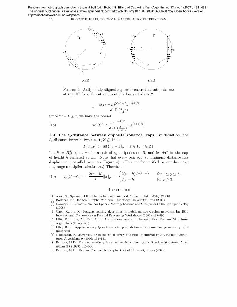
Figure 4. Antipodally aligned caps ±C centered at antipodes ±aof B ⊆ R
2 for different values of p below and above 2.
=π(2r − h)(d−1)/2h(d+1)/2
d · Γ(
d+12
) .
Since 2r − h ≥ r, we have the bound
(18) vol(C) ≥ πr(d−1)/2
d · Γ(
d+12
) · h(d+1)/2.
A.4. The `p-distance between opposite spherical caps. By definition, the`p-distance between two sets Y, Z ⊆ R
d is
dp(Y, Z) := inf{‖y − z‖p : y ∈ Y, z ∈ Z}.Let B = Bd
2 (r), let ±a be a pair of `p-antipodes on B, and let ±C be the capof height h centered at ±a. Note that every pair y, z at minimum distance hasdisplacement parallel to a (see Figure 4). (This can be verified by another easyLagrange-multiplier calculation.) Therefore
(19) dp(C,−C) =2(r − h)
r‖a‖p =
{
2(r − h)d1/p−1/2 for 1 ≤ p ≤ 2,
2(r − h) for p ≥ 2.
References
[1] Alon, N., Spencer, J.H.: The probabilistic method. 2nd edn. John Wiley (2000)[2] Bollobas, B.: Random Graphs. 2nd edn. Cambridge University Press (2001)[3] Conway, J.H., Sloane, N.J.A.: Sphere Packing, Lattices and Groups. 3rd edn. Springer-Verlag
(1998)[4] Chen, X., Jia, X.: Package routing algorithms in mobile ad-hoc wireless networks. In: 2001
International Conference on Parallel Processing Workshops. (2001) 485–490[5] Ellis, R.B., Jia, X., Yan, C.H.: On random points in the unit disk. Random Structures
Algorithms (to appear)[6] Ellis, R.B.: Approximating `p-metrics with path distance in a random geometric graph.
(preprint)[7] Godehardt, E., Jaworski, J: On the connectivity of a random interval graph. Random Struc-
tures Algorithms 9 (1996) 137–161[8] Penrose, M.D.: On k-connectivity for a geometric random graph. Random Structures Algo-
rithms 15 (1999) 145–164[9] Penrose, M.D.: Random Geometric Graphs. Oxford University Press (2003)
Random geometric graph diameter in the unit ball (with Robert B. Ellis and Catherine Yan) Algorithmica 47, no. 4 (2007), 421--438. The original publication is available at www.springerlink.com: http://dx.doi.org/10.1007/s00453-006-0172-y Open Access version: http://kuscholarworks.ku.edu/dspace/.
RANDOM GEOMETRIC GRAPH DIAMETER 17
[10] Stojmenovic, I., Seddigh, M., Zunic, J.: Dominating sets and neighbor elimination-basedbroadcasting algorithms in wireless networks. IEEE Trans. Parallel Distrib. Syst. 13 (2002)14–25
[11] Whittaker, E.T., Watson, G.N.: A course of modern analysis. Cambridge University Press(1996)
[12] Wu, J., Li, H.: A dominating-set-based routing scheme in ad hoc wireless networks. Telecom-munication Systems 18 (2001) 13–36
Department of Applied Mathematics, Illinois Institute of Technology, Chicago, IL
60616, USA
E-mail address: [email protected]
Department of Mathematics, University of Kansas, Lawrence, KS 66045-7523
E-mail address: [email protected]
Department of Mathematics, Texas A&M University, College Station, TX 77843-
3368, USA
E-mail address: [email protected]
Random geometric graph diameter in the unit ball (with Robert B. Ellis and Catherine Yan) Algorithmica 47, no. 4 (2007), 421--438. The original publication is available at www.springerlink.com: http://dx.doi.org/10.1007/s00453-006-0172-y Open Access version: http://kuscholarworks.ku.edu/dspace/.