
RELIABILITY IN SOFTWARE ENGINEERING QUALITATIVE RESEARCH ...
QUALITATIVE PROPERTIES OF α-FAIR POLICIES INBANDWIDTH-SHARING NETWORKS
By D. Shah and J. N. Tsitsiklis and Y. Zhong∗
Massachusetts Institute of Technology,University of California, Berkeley
We consider a flow-level model of a network operating under anα-fair bandwidth sharing policy (with α > 0) proposed by Robertsand Massoulie (2000). This is a probabilistic model that captures thelong-term aspects of bandwidth sharing between users or flows in acommunication network.
We study the transient properties as well as the steady-state dis-tribution of the model. In particular, for α ≥ 1, we obtain boundson the maximum number of flows in the network over a given timehorizon, by means of a maximal inequality derived from the standardLyapunov drift condition. As a corollary, we establish the full statespace collapse property for all α ≥ 1.
For the steady-state distribution, we obtain explicit exponentialtail bounds on the number of flows, for any α > 0, by relying on anorm-like Lyapunov function. As a corollary, we establish the validityof the diffusion approximation developed by Kang et al (2009), insteady state, for the case where α = 1 and under a local trafficcondtion.
1. Introduction. We consider a flow-level model of a network that op-erates under an α-fair bandwidth-sharing policy, and establish a variety ofnew results on the resulting performance. These results include tail boundson the size of a maximal excursion during a finite time interval, finitenessof expected queue sizes, exponential tail bounds under the steady-state dis-tribution, and the validity of the heavy-traffic diffusion approximation insteady state. We note that our results are to a great extent parallel and com-plementary to our work on packet-switched networks, which was reported
∗April 12, 2011; revised September 2012. This work was supported by NSF projectCCF-0728554. The first two authors are affiliated with the Laboratory for Informationand Decision Systems as well as the Operations Research Center at MIT. The last authoris affiliated with the Algorithms, Machines and People’s Laboratory at the Universityof California, Berkeley. Emails: devavrat,[email protected], [email protected]. Theauthors are grateful to Kuang Xu for reading the manuscript and his comments.
AMS 2000 subject classifications: Primary 60K20, 68M12; Secondary 68M20Keywords and phrases: Bandwidth-Sharing Policy, State Space Collapse, α-fair, Heavy
Traffic
1
2 SHAH & TSITSIKLIS & ZHONG
in [18].In the remainder of this section, we put our results in perspective by
comparing them with earlier work, and conclude with some more details onthe nature of our contributions.
1.1. Background. The flow-level network model that we consider wasintroduced by Roberts and Massoulie [17] to study the dynamic behavior ofInternet flows. It builds on a static version of the model that was proposedearlier by Kelly, Maulloo, and Tan [15], and subsequently generalized byMo and Walrand [16] who introduced a class of “fair” bandwidth-sharingpolicies parameterized by α > 0.
The most basic question regarding flow-level models concerns necessaryand sufficient conditions for stability, that is, for the existence of a steady-state distribution for the associated Markov process. This question was an-swered by Bonald and Massoulie [4] for the case of α-fair policies with α > 0,and by de Veciana et al. [6] for the case of max-min fair policies (α → ∞)and proportionally fair (α = 1) policies. In all cases, the stability conditionsturned out to be the natural deterministic conditions based on mean arrivaland service rates.
Given these stability results, the natural next question is whether thesteady-state expectation of the number of flows in the system is finite andif so, to identify some nontrivial upper bounds. When α ≥ 1, the finitenessquestion can be answered in the affirmative, and explicit bounds can beobtained, by exploiting the same Lyapunov drift inequality that had beenused in earlier work to establish stability. However, this approach does notseem to apply to the case where α ∈ (0, 1), which remained an open problem;this is one of the problems that we settle in this paper.
A more refined analysis of the number of flows present in the system con-cerns exponentially decaying bounds on the tail of its steady-state distribu-tion. We provide results of this form, together with explicit bounds for theassociated exponent. While a result of this type was not previously available,we take note of related recent results by Stolyar [21] and Venkataramananand Lin [23] who provide a precise asymptotic characterization of the expo-nent of the tail probability, in steady state, for the case of switched networks(as opposed to flow-level network models). (To be precise, their results con-cern the (1 + α) norm of the vector of flow counts under maximum weightor pressure policies parameterized by α > 0.) We believe that their meth-ods extend to the model considered here, without much difficulty. However,their approach leads to a variational characterization that appears to bedifficult to evaluate (or even bound) explicitly. We also take note of work by
3
Subramanian [22], who establishes a large deviations principle for a class ofswitched network models under maximum weight or pressure policies withα = 1.
The analysis of the steady-state distribution for underloaded networksprovides only partial insights about the transient behavior of the associatedMarkov process. As an alternative, the heavy-traffic (or diffusion) scalingof the network can lead to parsimonious approximations for the transientbehavior. A general two-stage program for developing such diffusion approx-imations has been put forth by Bramson [5] and Williams [24], and has beencarried out in detail for certain particular classes of queueing network mod-els. To carry out this program, one needs to: (i) provide a detailed analysis ofa related fluid model when the network is critically loaded; and, (ii) identifya unique distributional limit of the associated diffusion-scaled processes bystudying a related Skorohod problem. The first stage of the program wascarried out by Kelly and Williams [14] who identified the invariant manifoldof the associated critically loaded fluid model. This further led to the proofby Kang et al. [13] of a multiplicative state space collapse property, simi-lar to results by Bramson [5]. We note that the above summarized resultshold under α-fair policies with an arbitrary α > 0. The second stage of theprogram has been carried out for the proportionally fair policy (α = 1) byKang et al. [13], under a technical local traffic condition, and more recently,by Ye and Yao [25], under a somewhat less restrictive technical condition.We note however that when α 6= 1, a diffusion approximation has not beenestablished. In this case, it is of interest to see at least whether propertiesthat are stronger than multiplicative state space collapse can be derived,something that is accomplished in the present paper.
The above outlined diffusion approximation results involve rigorous state-ments on the finite-time behavior of the original process. Kang et al. [13]further established that for the particular setting that they consider, theresulting diffusion approximation has an elegant product-form steady-statedistribution; this result gives rise to an intuitively appealing interpretationof the relation between the congestion control protocol utilized by the flows(the end-users) and the queues formed inside the network. It is natural toexpect that this product-form steady-state distribution is the limit of thesteady-state distributions in the original model under the diffusion scaling.Results of this type are known for certain queueing systems such as gen-eralized Jackson networks; see the work by Gamarnik and Zeevi [10]. Onthe other hand, the validity of such a steady-state diffusion approximationwas not known for the model considered in [13]; it will be established in thepresent paper.
4 SHAH & TSITSIKLIS & ZHONG
1.2. Our contributions. In this paper, we advance the performance anal-ysis of flow-level models of networks operating under an α-fair policy, inboth the steady-state and the transient regimes.
For the transient regime, we obtain a probabilistic bound on the maximal(over a finite time horizon) number of flows, when operating under an α-fair policy with α ≥ 1. This result is obtained by combining a Lyapunovdrift inequality with a natural extension of Doob’s maximal inequality fornon-negative supermartingales. Our probabilistic bound, together with priorresults on multiplicative state space collapse, leads immediately to a strongerproperty, namely, full state space collapse, for the case where α ≥ 1.
For the steady-state regime, we obtain non-asymptotic and explicit boundson the tail of the distribution of the number of flows, for any α > 0. In theprocess, we establish that, for any α > 0, all moments of the steady-statenumber of flows are finite. These results are proved by working with a normedversion of the Lyapunov function that was used in prior work. Specifically,we establish that this normed version is also a Lyapunov function for thesystem (i.e., it satisfies a drift inequality). It also happens to be a Lipschitzcontinuous function and this helps crucially in establishing exponential tailbounds, using results of Hajek [12] and Bertsimas et al. [2].
The exponent in the exponential tail bound that we establish for thedistribution of the number of flows is proportional to a suitably defineddistance (“gap”) from critical loading; this gap is of the same type as thefamiliar 1 − ρ term, where ρ is the usual load factor in a queueing system.This particular dependence on the load leads to the tightness of the steady-state distributions of the model under diffusion scaling. It leads to one of ourmain results, namely, the validity of the diffusion approximation, in steadystate, when α = 1 and a local traffic condition holds.
1.3. Organization. The rest of the paper is organized as follows. In Sec-tion 2, we define the notation and some of the terminology that we will em-ploy. We also describe the flow-level network model, as well as the weightedα-fair bandwidth-sharing policies. In Section 3, we provide formal statementsof our main results. The transient analysis is presented in Section 4. We startwith a general lemma, and specialize it to obtain a maximal inequality underα-fair policies, when α ≥ 1. We then apply the latter inequality to prove fullstate space collapse when α ≥ 1.
We then proceed to the steady-state analysis. In Section 5, we establisha drift inequality for a suitable Lyapunov function, which is central to ourproof of exponential upper bounds on tail probabilities We prove the ex-ponential upper bound on tail probabilities in Section 6. The validity of
5
the heavy-traffic steady-state approximation is established in Section 7. Weconclude the paper with a brief discussion in Section 8.
2. Model and Notation.
2.1. Notation. We introduce here the notation that will be employedthroughout the paper. We denote the real vector space of dimension M byRM , the set of nonnegative M -tuples by RM+ , and the set of positive M -tuples by RMp . We write R for R1, R+ for R1
+, and Rp for R1p. We let Z
be the set of integers, Z+ the set of nonnegative integers, and N the set ofpositive integers. Throughout the paper, we reserve bold letters for vectorsand plain letters for scalars.
For any vector x ∈ RM , and any α > 0, we define
‖x‖α =
(M∑i=1
|xi|α)1/α
,
and we define ‖x‖∞ = maxi∈1,...,M |xi|. For any two vectors x = (xi)Mi=1
and y = (yi)Mi=1 of the same dimensions, we let 〈x,y〉 =
∑Mi=1 xiyi be the
inner product of x and y. We let ei be the i-th unit vector in RM , and 1the vector of all ones. For a set S, we denote its cardinality by |S|, and itsindicator function by IS . For a matrix A, we let AT denote its transpose.
2.2. Flow-Level Network Model.
The Model. We adopt the model and notation in [14]. As explained indetail in [14], this model faithfully captures the long-term (or macro level)behavior of congestion control in the current Internet.
Let time be continuous and indexed by t ∈ R+. Consider a network witha finite set J of resources and a set I of routes, where a route is identifiedwith a non-empty subset of the resource set J . Let A be the |J | × |I|matrix with Aji = 1 if resource j is used by route i, and Aji = 0 otherwise.Assume that A has rank |J |. Let C = (Cj)j∈J be a capacity vector, wherewe assume that each entry Cj is a given positive constant. Let the numberof flows on route i at time t be denoted by Ni(t), and define the flow vectorat time t by N(t) = (Ni(t))i∈I . For each route i, new flows arrive as anindependent Poisson process of rate νi. Each arriving flow brings an amountof work (data that it wishes to transfer) which is an exponentially distributedrandom variable with mean 1/µi, independent of everything else. Each flowgets service from the network according to a bandwidth-sharing policy. Oncea flow is served, it departs the network.
6 SHAH & TSITSIKLIS & ZHONG
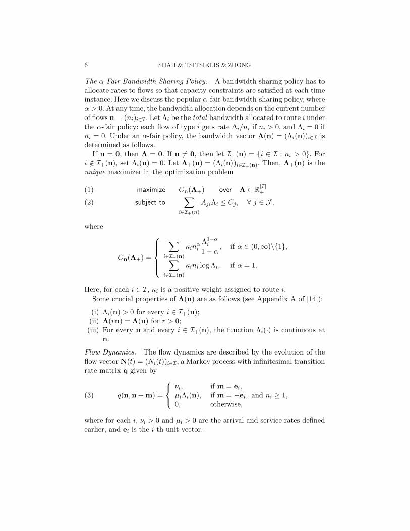
The α-Fair Bandwidth-Sharing Policy. A bandwidth sharing policy has toallocate rates to flows so that capacity constraints are satisfied at each timeinstance. Here we discuss the popular α-fair bandwidth-sharing policy, whereα > 0. At any time, the bandwidth allocation depends on the current numberof flows n = (ni)i∈I . Let Λi be the total bandwidth allocated to route i underthe α-fair policy: each flow of type i gets rate Λi/ni if ni > 0, and Λi = 0 ifni = 0. Under an α-fair policy, the bandwidth vector Λ(n) = (Λi(n))i∈I isdetermined as follows.
If n = 0, then Λ = 0. If n 6= 0, then let I+(n) = i ∈ I : ni > 0. Fori /∈ I+(n), set Λi(n) = 0. Let Λ+(n) = (Λi(n))i∈I+(n). Then, Λ+(n) is theunique maximizer in the optimization problem
maximize Gn(Λ+) over Λ ∈ R|I|+(1)
subject to∑
i∈I+(n)
AjiΛi ≤ Cj , ∀ j ∈ J ,(2)
where
Gn(Λ+) =
∑
i∈I+(n)
κinαi
Λ1−αi
1− α, if α ∈ (0,∞)\1,∑
i∈I+(n)
κini log Λi, if α = 1.
Here, for each i ∈ I, κi is a positive weight assigned to route i.Some crucial properties of Λ(n) are as follows (see Appendix A of [14]):
(i) Λi(n) > 0 for every i ∈ I+(n);(ii) Λ(rn) = Λ(n) for r > 0;(iii) For every n and every i ∈ I+(n), the function Λi(·) is continuous at
n.
Flow Dynamics. The flow dynamics are described by the evolution of theflow vector N(t) = (Ni(t))i∈I , a Markov process with infinitesimal transitionrate matrix q given by
(3) q(n,n + m) =
νi, if m = ei,µiΛi(n), if m = −ei, and ni ≥ 1,0, otherwise,
where for each i, νi > 0 and µi > 0 are the arrival and service rates definedearlier, and ei is the i-th unit vector.
7
Capacity Region. Flows of type i bring to the system an average of ρi =νi/µi units of work per unit time. Therefore, in order for the Markov processN(·) to be positive recurrent, it is necessary that
Aρ < C, componentwise.(4)
We note that under the α-fair bandwidth-sharing policy, Condition (4) isalso sufficient for positive recurrence of the process N(·) [4, 6, 14].
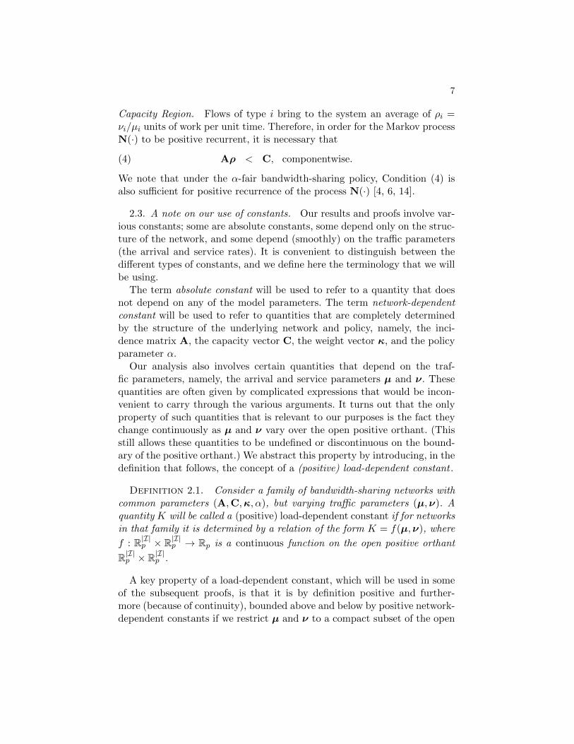
2.3. A note on our use of constants. Our results and proofs involve var-ious constants; some are absolute constants, some depend only on the struc-ture of the network, and some depend (smoothly) on the traffic parameters(the arrival and service rates). It is convenient to distinguish between thedifferent types of constants, and we define here the terminology that we willbe using.
The term absolute constant will be used to refer to a quantity that doesnot depend on any of the model parameters. The term network-dependentconstant will be used to refer to quantities that are completely determinedby the structure of the underlying network and policy, namely, the inci-dence matrix A, the capacity vector C, the weight vector κ, and the policyparameter α.
Our analysis also involves certain quantities that depend on the traf-fic parameters, namely, the arrival and service parameters µ and ν. Thesequantities are often given by complicated expressions that would be incon-venient to carry through the various arguments. It turns out that the onlyproperty of such quantities that is relevant to our purposes is the fact theychange continuously as µ and ν vary over the open positive orthant. (Thisstill allows these quantities to be undefined or discontinuous on the bound-ary of the positive orthant.) We abstract this property by introducing, in thedefinition that follows, the concept of a (positive) load-dependent constant .
Definition 2.1. Consider a family of bandwidth-sharing networks withcommon parameters (A,C,κ, α), but varying traffic parameters (µ,ν). Aquantity K will be called a (positive) load-dependent constant if for networksin that family it is determined by a relation of the form K = f(µ,ν), where
f : R|I|p × R|I|p → Rp is a continuous function on the open positive orthant
R|I|p × R|I|p .
A key property of a load-dependent constant, which will be used in someof the subsequent proofs, is that it is by definition positive and further-more (because of continuity), bounded above and below by positive network-dependent constants if we restrict µ and ν to a compact subset of the open
8 SHAH & TSITSIKLIS & ZHONG
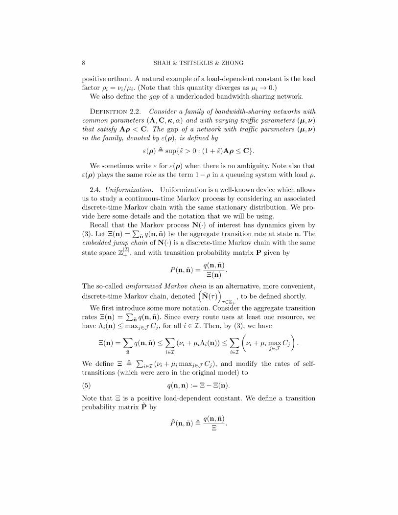
positive orthant. A natural example of a load-dependent constant is the loadfactor ρi = νi/µi. (Note that this quantity diverges as µi → 0.)
We also define the gap of a underloaded bandwidth-sharing network.
Definition 2.2. Consider a family of bandwidth-sharing networks withcommon parameters (A,C,κ, α) and with varying traffic parameters (µ,ν)that satisfy Aρ < C. The gap of a network with traffic parameters (µ,ν)in the family, denoted by ε(ρ), is defined by
ε(ρ) , supε > 0 : (1 + ε)Aρ ≤ C.
We sometimes write ε for ε(ρ) when there is no ambiguity. Note also thatε(ρ) plays the same role as the term 1−ρ in a queueing system with load ρ.
2.4. Uniformization. Uniformization is a well-known device which allowsus to study a continuous-time Markov process by considering an associateddiscrete-time Markov chain with the same stationary distribution. We pro-vide here some details and the notation that we will be using.
Recall that the Markov process N(·) of interest has dynamics given by(3). Let Ξ(n) =
∑n q(n, n) be the aggregate transition rate at state n. The
embedded jump chain of N(·) is a discrete-time Markov chain with the same
state space Z|I|+ , and with transition probability matrix P given by
P (n, n) =q(n, n)
Ξ(n).
The so-called uniformized Markov chain is an alternative, more convenient,
discrete-time Markov chain, denoted(N(τ)
)τ∈Z+
, to be defined shortly.
We first introduce some more notation. Consider the aggregate transitionrates Ξ(n) =
∑n q(n, n). Since every route uses at least one resource, we
have Λi(n) ≤ maxj∈J Cj , for all i ∈ I. Then, by (3), we have
Ξ(n) =∑n
q(n, n) ≤∑i∈I
(νi + µiΛi(n)) ≤∑i∈I
(νi + µi max
j∈JCj
).
We define Ξ ,∑
i∈I (νi + µi maxj∈J Cj), and modify the rates of self-transitions (which were zero in the original model) to
(5) q(n,n) := Ξ− Ξ(n).
Note that Ξ is a positive load-dependent constant. We define a transitionprobability matrix P by
P (n, n) ,q(n, n)
Ξ.
9
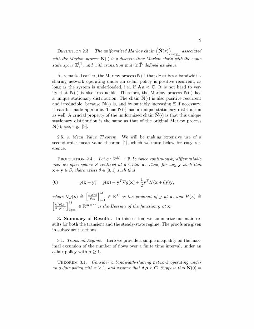
Definition 2.3. The uniformized Markov chain(N(τ)
)τ∈Z+
associated
with the Markov process N(·) is a discrete-time Markov chain with the same
state space Z|I|+ , and with transition matrix P defined as above.
As remarked earlier, the Markov process N(·) that describes a bandwidth-sharing network operating under an α-fair policy is positive recurrent, aslong as the system is underloaded, i.e., if Aρ < C. It is not hard to ver-ify that N(·) is also irreducible. Therefore, the Markov process N(·) hasa unique stationary distribution. The chain N(·) is also positive recurrentand irreducible, because N(·) is, and by suitably increasing Ξ if necessary,it can be made aperiodic. Thus N(·) has a unique stationary distributionas well. A crucial property of the uniformized chain N(·) is that this uniquestationary distribution is the same as that of the original Markov processN(·); see, e.g., [9].
2.5. A Mean Value Theorem. We will be making extensive use of asecond-order mean value theorem [1], which we state below for easy ref-erence.
Proposition 2.4. Let g : RM → R be twice continuously differentiableover an open sphere S centered at a vector x. Then, for any y such thatx + y ∈ S, there exists θ ∈ [0, 1] such that
(6) g(x + y) = g(x) + yT∇g(x) +1
2yTH(x + θy)y,
where ∇g(x) ,[∂g(x)∂xi
]Mi=1∈ RM is the gradient of g at x, and H(x) ,[
∂2g(x)∂xi∂xj
]Mi,j=1
∈ RM×M is the Hessian of the function g at x.
3. Summary of Results. In this section, we summarize our main re-sults for both the transient and the steady-state regime. The proofs are givenin subsequent sections.
3.1. Transient Regime. Here we provide a simple inequality on the max-imal excursion of the number of flows over a finite time interval, under anα-fair policy with α ≥ 1.
Theorem 3.1. Consider a bandwidth-sharing network operating underan α-fair policy with α ≥ 1, and assume that Aρ < C. Suppose that N(0) =
10 SHAH & TSITSIKLIS & ZHONG
0. Let N∗(T ) = supt∈[0,T ],i∈I Ni(t), and let ε be the gap. Then, for any b > 0,
(7) P (N∗(T ) ≥ b) ≤ KT
εα−1bα+1,
for some positive load-dependent constant K.
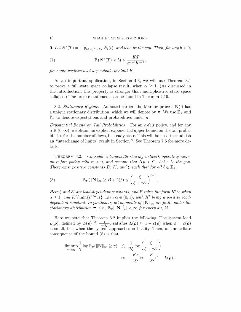
As an important application, in Section 4.3, we will use Theorem 3.1to prove a full state space collapse result, when α ≥ 1. (As discussed inthe introduction, this property is stronger than multiplicative state spacecollapse.) The precise statement can be found in Theorem 4.10.
3.2. Stationary Regime. As noted earlier, the Markov process N(·) hasa unique stationary distribution, which we will denote by π. We use Eπ andPπ to denote expectations and probabilities under π.
Exponential Bound on Tail Probabilities. For an α-fair policy, and for anyα ∈ (0,∞), we obtain an explicit exponential upper bound on the tail proba-bilities for the number of flows, in steady state. This will be used to establishan “interchange of limits” result in Section 7. See Theorem 7.6 for more de-tails.
Theorem 3.2. Consider a bandwidth-sharing network operating underan α-fair policy with α > 0, and assume that Aρ < C. Let ε be the gap.There exist positive constants B, K, and ξ such that for all ` ∈ Z+:
(8) Pπ (‖N‖∞ ≥ B + 2ξ`) ≤(
ξ
ξ + εK
)`+1
.
Here ξ and K are load-dependent constants, and B takes the form K ′/ε whenα ≥ 1, and K ′/minε1/α, ε when α ∈ (0, 1), with K ′ being a positive load-dependent constant. In particular, all moments of ‖N‖∞ are finite under thestationary distribution π, i.e., Eπ[‖N‖k∞] <∞ for every k ∈ N.
Here we note that Theorem 3.2 implies the following. The system loadL(ρ), defined by L(ρ) , 1
1+ε(ρ) , satisfies L(ρ) ≈ 1 − ε(ρ) when ε = ε(ρ)is small, i.e., when the system approaches criticality. Then, an immediateconsequence of the bound (8) is that
lim supγ→∞
1
γlogPπ(‖N‖∞ ≥ γ) .
1
2ξlog
(ξ
ξ + εK
)≈ −Kε
2ξ2≈ − K
2ξ2(1− L(ρ)).
11
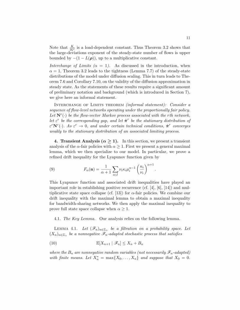
Note that K2ξ2
is a load-dependent constant. Thus Theorem 3.2 shows thatthe large-deviations exponent of the steady-state number of flows is upperbounded by −(1− L(ρ)), up to a multiplicative constant.
Interchange of Limits (α = 1). As discussed in the introduction, whenα = 1, Theorem 3.2 leads to the tightness (Lemma 7.7) of the steady-statedistributions of the model under diffusion scaling. This in turn leads to The-orem 7.6 and Corollary 7.10, on the validity of the diffusion approximation insteady state. As the statements of these results require a significant amountof preliminary notation and background (which is introduced in Section 7),we give here an informal statement.
Interchange of Limits theorem (informal statement): Consider asequence of flow-level networks operating under the proportionally fair policy.Let Nr(·) be the flow-vector Markov process associated with the rth network,let εr be the corresponding gap, and let πr be the stationary distribution ofεrNr(·). As εr → 0, and under certain technical conditions, πr convergesweakly to the stationary distribution of an associated limiting process.
4. Transient Analysis (α ≥ 1). In this section, we present a transientanalysis of the α-fair policies with α ≥ 1. First we present a general maximallemma, which we then specialize to our model. In particular, we prove arefined drift inequality for the Lyapunov function given by
(9) Fα(n) =1
α+ 1
∑i∈I
νiκiµα−1i
(niνi
)α+1
.
This Lyapunov function and associated drift inequalities have played animportant role in establishing positive recurrence (cf. [4], [6], [14]) and mul-tiplicative state space collapse (cf. [13]) for α-fair policies. We combine ourdrift inequality with the maximal lemma to obtain a maximal inequalityfor bandwidth-sharing networks. We then apply the maximal inequality toprove full state space collapse when α ≥ 1.
4.1. The Key Lemma. Our analysis relies on the following lemma.
Lemma 4.1. Let (Fn)n∈Z+ be a filtration on a probability space. Let(Xn)n∈Z+ be a nonnegative Fn-adapted stochastic process that satisfies
(10) E[Xn+1 | Fn] ≤ Xn +Bn
where the Bn are nonnegative random variables (not necessarily Fn-adapted)with finite means. Let X∗n = maxX0, . . . , Xn and suppose that X0 = 0.
12 SHAH & TSITSIKLIS & ZHONG
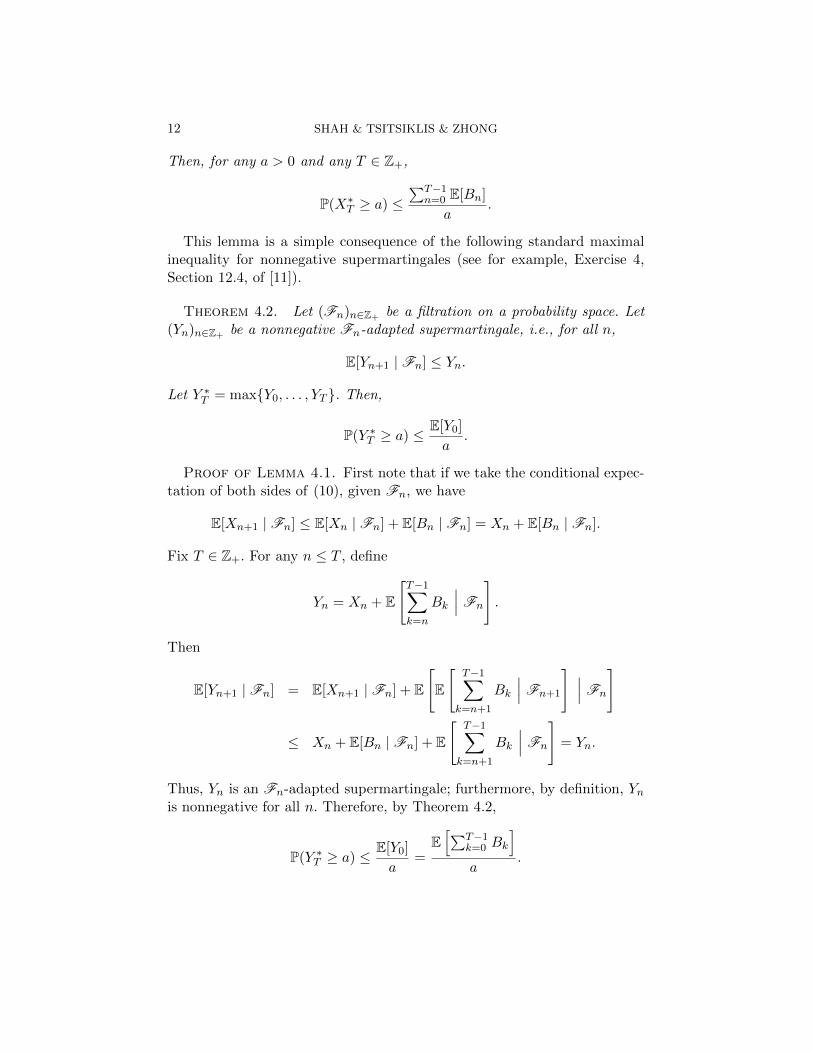
Then, for any a > 0 and any T ∈ Z+,
P(X∗T ≥ a) ≤∑T−1
n=0 E[Bn]
a.
This lemma is a simple consequence of the following standard maximalinequality for nonnegative supermartingales (see for example, Exercise 4,Section 12.4, of [11]).
Theorem 4.2. Let (Fn)n∈Z+ be a filtration on a probability space. Let(Yn)n∈Z+ be a nonnegative Fn-adapted supermartingale, i.e., for all n,
E[Yn+1 | Fn] ≤ Yn.
Let Y ∗T = maxY0, . . . , YT . Then,
P(Y ∗T ≥ a) ≤ E[Y0]
a.
Proof of Lemma 4.1. First note that if we take the conditional expec-tation of both sides of (10), given Fn, we have
E[Xn+1 | Fn] ≤ E[Xn | Fn] + E[Bn | Fn] = Xn + E[Bn | Fn].
Fix T ∈ Z+. For any n ≤ T , define
Yn = Xn + E
[T−1∑k=n
Bk
∣∣∣ Fn
].
Then
E[Yn+1 | Fn] = E[Xn+1 | Fn] + E
[E
[T−1∑k=n+1
Bk
∣∣∣ Fn+1
] ∣∣∣ Fn
]
≤ Xn + E[Bn | Fn] + E
[T−1∑k=n+1
Bk
∣∣∣ Fn
]= Yn.
Thus, Yn is an Fn-adapted supermartingale; furthermore, by definition, Ynis nonnegative for all n. Therefore, by Theorem 4.2,
P(Y ∗T ≥ a) ≤ E[Y0]
a=
E[∑T−1
k=0 Bk
]a
.
13
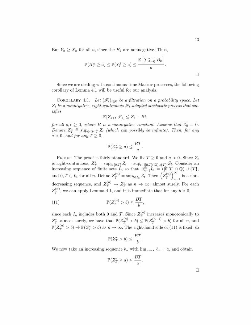
But Yn ≥ Xn for all n, since the Bk are nonnegative. Thus,
P(X∗T ≥ a) ≤ P(Y ∗T ≥ a) ≤E[∑T−1
k=0 Bk
]a
.
Since we are dealing with continuous-time Markov processes, the followingcorollary of Lemma 4.1 will be useful for our analysis.
Corollary 4.3. Let (Ft)t≥0 be a filtration on a probability space. LetZt be a nonnegative, right-continuous Ft-adapted stochastic process that sat-isfies
E[Zs+t|Fs] ≤ Zs +Bt,
for all s, t ≥ 0, where B is a nonnegative constant. Assume that Z0 ≡ 0.Denote Z∗T , sup0≤t≤T Zt (which can possibly be infinite). Then, for anya > 0, and for any T ≥ 0,
P(Z∗T ≥ a) ≤ BT
a.
Proof. The proof is fairly standard. We fix T ≥ 0 and a > 0. Since Ztis right-continuous, Z∗T = supt∈[0,T ] Zt = supt∈([0,T ]∩Q)∪T Zt. Consider anincreasing sequence of finite sets In so that ∪∞n=1In = ([0, T ] ∩ Q) ∪ T,and 0, T ∈ In for all n. Define Z
(n)T = supt∈In Zt. Then
(Z
(n)T
)∞n=1
is a non-
decreasing sequence, and Z(n)T → Z∗T as n → ∞, almost surely. For each
Z(n)T , we can apply Lemma 4.1, and it is immediate that for any b > 0,
(11) P(Z(n)T > b) ≤ BT
b,
since each In includes both 0 and T . Since Z(n)T increases monotonically to
Z∗T , almost surely, we have that P(Z(n)T > b) ≤ P(Z
(n+1)T > b) for all n, and
P(Z(n)T > b)→ P(Z∗T > b) as n→∞. The right-hand side of (11) is fixed, so
P(Z∗T > b) ≤ BT
b.
We now take an increasing sequence bn with limn→∞ bn = a, and obtain
P(Z∗T ≥ a) ≤ BT
a.
14 SHAH & TSITSIKLIS & ZHONG
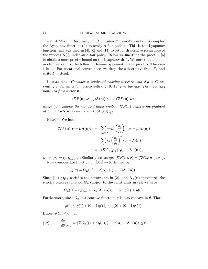
4.2. A Maximal Inequality for Bandwidth-Sharing Networks. We employthe Lyapunov function (9) to study α-fair policies. This is the Lyapunovfunction that was used in [4], [6] and [14] to establish positive recurrence ofthe process N(·) under an α-fair policy. Below we fine-tune the proof in [6]to obtain a more precise bound on the Lyapunov drift. We note that a “fluid-model” version of the following lemma appeared in the proof of Theorem1 in [4]. For notational convenience, we drop the subscript α from Fα andwrite F instead.
Lemma 4.4. Consider a bandwidth-sharing network with Aρ < C op-erating under an α-fair policy with α > 0. Let ε be the gap. Then, for anynon-zero flow vector n,
〈∇F (n),ν − µΛ(n)〉 ≤ −ε 〈∇F (n),ν〉 ,
where 〈·, ·〉 denotes the standard inner product, ∇F (n) denotes the gradientof F , and µΛ(n) is the vector (µiΛi(n))i∈I .
Proof. We have
〈∇F (n),ν − µΛ(n)〉 =∑i∈I
1
µiκi
(niρi
)α(νi − µiΛi(n))
=∑i∈I
κi
(niρi
)α(ρi − Λi(n))
=⟨∇Gn(ρ+),ρ+ −Λ+(n)
⟩,
where ρ+ = (ρi)i∈I+(n). Similarly we can get 〈∇F (n),ν〉 =⟨∇Gn(ρ+),ρ+
⟩.
Now consider the function g : [0, 1]→ R defined by
g(θ) = Gn
(θ(1 + ε)ρ+ + (1− θ)Λ+(n)
).
Since (1 + ε)ρ+ satisfies the constraints in (2), and Λ+(n) maximizes thestrictly concave function Gn subject to the constraints in (2), we have
Gn((1 + ε)ρ+) ≤ Gn(Λ+(n)), i.e., g(1) ≤ g(0).
Furthermore, since Gn is a concave function, g is also concave in θ. Thus,
g(0) ≤ g(1) + (0− 1)g′(1) ≤ g(0) + (0− 1)g′(1).
Hence, g′(1) ≤ 0, i.e.,
(12)dg
dθ
∣∣∣θ=1
=⟨∇Gn((1 + ε)ρ+), (1 + ε)ρ+ −Λ+(n)
⟩≤ 0.
15
But it is easy to check that∇Gn((1+ε)ρ+) = (1+ε)−α∇Gn(ρ+), so dividing(12) by (1 + ε)−α, we have⟨
∇Gn(ρ+),ρ+ −Λ+(n)⟩≤ −ε
⟨∇Gn(ρ+),ρ+
⟩.
This is the same as
〈∇F (n),ν − µΛ(n)〉 ≤ −ε 〈∇F (n),ν〉 .
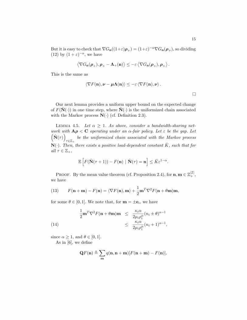
Our next lemma provides a uniform upper bound on the expected changeof F (N(·)) in one time step, where N(·) is the uniformized chain associatedwith the Markov process N(·) (cf. Definition 2.3).
Lemma 4.5. Let α ≥ 1. As above, consider a bandwidth-sharing net-work with Aρ < C operating under an α-fair policy. Let ε be the gap. Let(N(τ)
)τ∈Z+
be the uniformized chain associated with the Markov process
N(·). Then, there exists a positive load-dependent constant K, such that forall τ ∈ Z+,
E[F (N(τ + 1))− F (n) | N(τ) = n
]≤ Kε1−α.
Proof. By the mean value theorem (cf. Proposition 2.4), for n,m ∈ Z|I|+ ,we have
(13) F (n + m)− F (n) = 〈∇F (n),m〉+1
2mT∇2F (n + θm)m,
for some θ ∈ [0, 1]. We note that, for m = ±ei, we have
1
2mT∇2F (n + θm)m ≤ κiα
2µiραi(ni ± θ)α−1
≤ κiα
2µiραi(ni + 1)α−1,(14)
since α ≥ 1, and θ ∈ [0, 1].As in [6], we define
QF (n) ,∑m
q(n,n + m)[F (n + m)− F (n)],
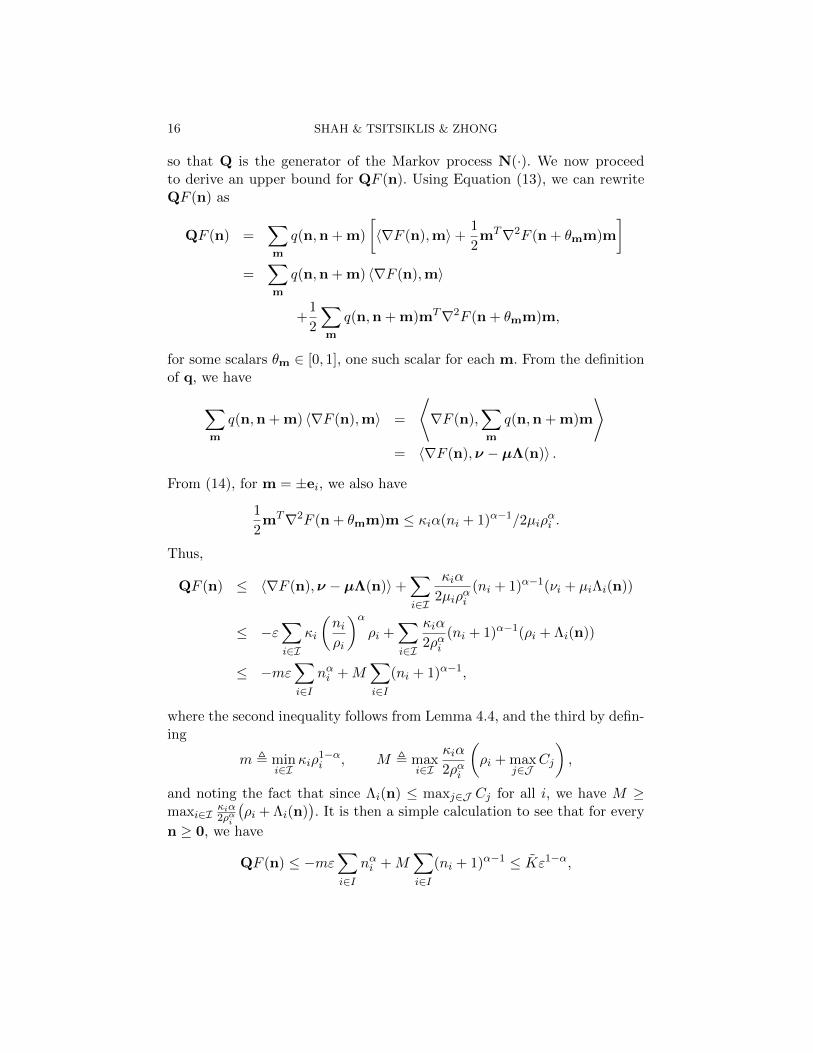
16 SHAH & TSITSIKLIS & ZHONG
so that Q is the generator of the Markov process N(·). We now proceedto derive an upper bound for QF (n). Using Equation (13), we can rewriteQF (n) as
QF (n) =∑m
q(n,n + m)
[〈∇F (n),m〉+
1
2mT∇2F (n + θmm)m
]=
∑m
q(n,n + m) 〈∇F (n),m〉
+1
2
∑m
q(n,n + m)mT∇2F (n + θmm)m,
for some scalars θm ∈ [0, 1], one such scalar for each m. From the definitionof q, we have
∑m
q(n,n + m) 〈∇F (n),m〉 =
⟨∇F (n),
∑m
q(n,n + m)m
⟩= 〈∇F (n),ν − µΛ(n)〉 .
From (14), for m = ±ei, we also have
1
2mT∇2F (n + θmm)m ≤ κiα(ni + 1)α−1/2µiρ
αi .
Thus,
QF (n) ≤ 〈∇F (n),ν − µΛ(n)〉+∑i∈I
κiα
2µiραi(ni + 1)α−1(νi + µiΛi(n))
≤ −ε∑i∈I
κi
(niρi
)αρi +
∑i∈I
κiα
2ραi(ni + 1)α−1(ρi + Λi(n))
≤ −mε∑i∈I
nαi +M∑i∈I
(ni + 1)α−1,
where the second inequality follows from Lemma 4.4, and the third by defin-ing
m , mini∈I
κiρ1−αi , M , max
i∈I
κiα
2ραi
(ρi + max
j∈JCj
),
and noting the fact that since Λi(n) ≤ maxj∈J Cj for all i, we have M ≥maxi∈I
κiα2ραi
(ρi + Λi(n)
). It is then a simple calculation to see that for every
n ≥ 0, we have
QF (n) ≤ −mε∑i∈I
nαi +M∑i∈I
(ni + 1)α−1 ≤ Kε1−α,
17
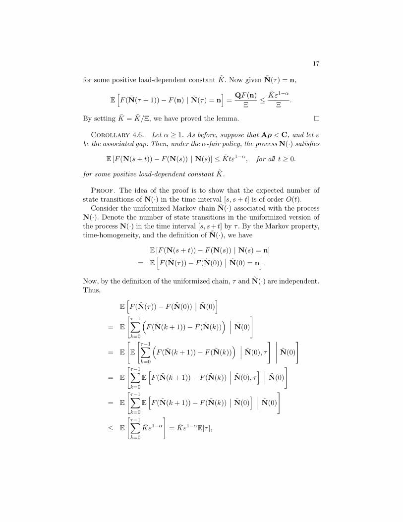
for some positive load-dependent constant K. Now given N(τ) = n,
E[F (N(τ + 1))− F (n) | N(τ) = n
]=
QF (n)
Ξ≤ Kε1−α
Ξ.
By setting K = K/Ξ, we have proved the lemma.
Corollary 4.6. Let α ≥ 1. As before, suppose that Aρ < C, and let εbe the associated gap. Then, under the α-fair policy, the process N(·) satisfies
E [F (N(s+ t))− F (N(s)) | N(s)] ≤ Ktε1−α, for all t ≥ 0.
for some positive load-dependent constant K.
Proof. The idea of the proof is to show that the expected number ofstate transitions of N(·) in the time interval [s, s+ t] is of order O(t).
Consider the uniformized Markov chain N(·) associated with the processN(·). Denote the number of state transitions in the uniformized version ofthe process N(·) in the time interval [s, s+ t] by τ . By the Markov property,time-homogeneity, and the definition of N(·), we have
E [F (N(s+ t))− F (N(s)) | N(s) = n]
= E[F (N(τ))− F (N(0))
∣∣ N(0) = n].
Now, by the definition of the uniformized chain, τ and N(·) are independent.Thus,
E[F (N(τ))− F (N(0))
∣∣ N(0)]
= E
[τ−1∑k=0
(F (N(k + 1))− F (N(k))
) ∣∣∣ N(0)
]
= E
[E
[τ−1∑k=0
(F (N(k + 1))− F (N(k))
) ∣∣∣ N(0), τ
] ∣∣∣∣∣ N(0)
]
= E
[τ−1∑k=0
E[F (N(k + 1))− F (N(k))
∣∣∣ N(0), τ] ∣∣∣ N(0)
]
= E
[τ−1∑k=0
E[F (N(k + 1))− F (N(k))
∣∣ N(0)] ∣∣∣ N(0)
]
≤ E
[τ−1∑k=0
Kε1−α
]= Kε1−αE[τ ],
18 SHAH & TSITSIKLIS & ZHONG
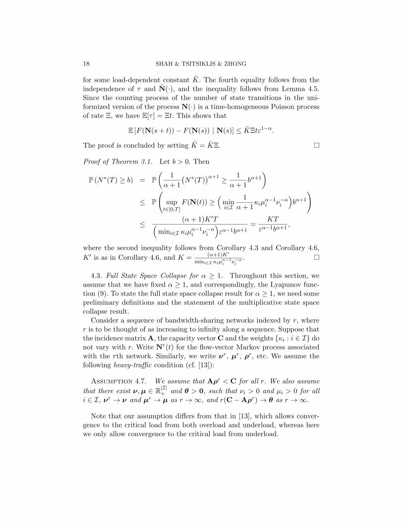
for some load-dependent constant K. The fourth equality follows from theindependence of τ and N(·), and the inequality follows from Lemma 4.5.Since the counting process of the number of state transitions in the uni-formized version of the process N(·) is a time-homogeneous Poisson processof rate Ξ, we have E[τ ] = Ξt. This shows that
E [F (N(s+ t))− F (N(s)) | N(s)] ≤ KΞtε1−α.
The proof is concluded by setting K = KΞ.
Proof of Theorem 3.1. Let b > 0. Then
P (N∗(T ) ≥ b) = P(
1
α+ 1
(N∗(T )
)α+1 ≥ 1
α+ 1bα+1
)≤ P
(supt∈[0,T ]
F (N(t)) ≥(
mini∈I
1
α+ 1κiµ
α−1i ν−αi
)bα+1
)
≤ (α+ 1)K ′T(mini∈I κiµ
α−1i ν−αi
)εα−1bα+1
=KT
εα−1bα+1,
where the second inequality follows from Corollary 4.3 and Corollary 4.6,
K ′ is as in Corollary 4.6, and K = (α+1)K′
mini∈I κiµα−1i ν−αi
.
4.3. Full State Space Collapse for α ≥ 1. Throughout this section, weassume that we have fixed α ≥ 1, and correspondingly, the Lyapunov func-tion (9). To state the full state space collapse result for α ≥ 1, we need somepreliminary definitions and the statement of the multiplicative state spacecollapse result.
Consider a sequence of bandwidth-sharing networks indexed by r, wherer is to be thought of as increasing to infinity along a sequence. Suppose thatthe incidence matrix A, the capacity vector C and the weights κi : i ∈ I donot vary with r. Write Nr(t) for the flow-vector Markov process associatedwith the rth network. Similarly, we write νr, µr, ρr, etc. We assume thefollowing heavy-traffic condition (cf. [13]):
Assumption 4.7. We assume that Aρr < C for all r. We also assume
that there exist ν,µ ∈ R|I|+ and θ > 0, such that νi > 0 and µi > 0 for alli ∈ I, νr → ν and µr → µ as r →∞, and r(C−Aρr)→ θ as r →∞.
Note that our assumption differs from that in [13], which allows conver-gence to the critical load from both overload and underload, whereas herewe only allow convergence to the critical load from underload.
19
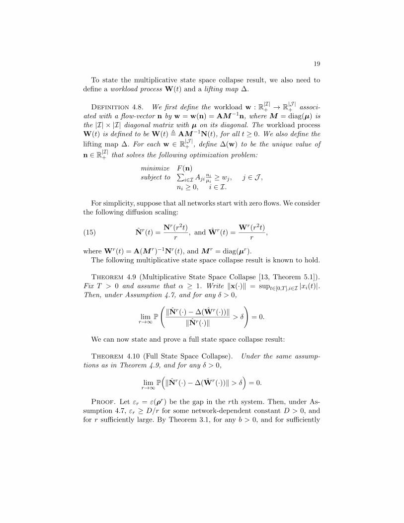
To state the multiplicative state space collapse result, we also need todefine a workload process W(t) and a lifting map ∆.
Definition 4.8. We first define the workload w : R|I|+ → R|J |+ associ-ated with a flow-vector n by w = w(n) = AM−1n, where M = diag(µ) isthe |I| × |I| diagonal matrix with µ on its diagonal. The workload processW(t) is defined to be W(t) , AM−1N(t), for all t ≥ 0. We also define the
lifting map ∆. For each w ∈ R|J |+ , define ∆(w) to be the unique value of
n ∈ R|I|+ that solves the following optimization problem:
minimize F (n)subject to
∑i∈I Aji
niµi≥ wj , j ∈ J ,
ni ≥ 0, i ∈ I.
For simplicity, suppose that all networks start with zero flows. We considerthe following diffusion scaling:
(15) Nr(t) =Nr(r2t)
r, and Wr(t) =
Wr(r2t)
r,
where Wr(t) = A(M r)−1Nr(t), and M r = diag(µr).The following multiplicative state space collapse result is known to hold.
Theorem 4.9 (Multiplicative State Space Collapse [13, Theorem 5.1]).Fix T > 0 and assume that α ≥ 1. Write ‖x(·)‖ = supt∈[0,T ],i∈I |xi(t)|.Then, under Assumption 4.7, and for any δ > 0,
limr→∞
P
(‖Nr(·)−∆(Wr(·))‖
‖Nr(·)‖> δ
)= 0.
We can now state and prove a full state space collapse result:
Theorem 4.10 (Full State Space Collapse). Under the same assump-tions as in Theorem 4.9, and for any δ > 0,
limr→∞
P(‖Nr(·)−∆(Wr(·))‖ > δ
)= 0.
Proof. Let εr = ε(ρr) be the gap in the rth system. Then, under As-sumption 4.7, εr ≥ D/r for some network-dependent constant D > 0, andfor r sufficiently large. By Theorem 3.1, for any b > 0, and for sufficiently
20 SHAH & TSITSIKLIS & ZHONG
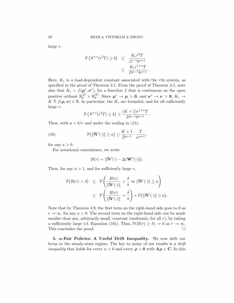
large r,
P(N r,∗(r2T ) ≥ b
)≤ Krr
2T
εα−1r bα+1
≤ Krr1+αT
Dα−1bα+1.
Here, Kr is a load-dependent constant associated with the rth system, asspecified in the proof of Theorem 3.1. From the proof of Theorem 3.1, notealso that Kr = f(µr,νr), for a function f that is continuous on the open
positive orthant R|I|p × R|I|p . Since µr → µ > 0, and νr → ν > 0, Kr →K , f(µ,ν) ∈ R. In particular, the Kr are bounded, and for all sufficientlylarge r,
P(N r,∗(r2T ) ≥ b
)≤ (K + 1)r1+αT
Dα−1bα+1.
Then, with a = b/r and under the scaling in (15),
(16) P(‖Nr(·)‖ ≥ a
)≤ K + 1
Dα−1 ·T
aα+1,
for any a > 0.For notational convenience, we write
B(r) = ‖Nr(·)−∆(Wr(·))‖.
Then, for any a > 1, and for sufficiently large r,
P(B(r) > δ
)≤ P
(B(r)
‖Nr(·)‖>δ
aor ‖Nr(·)‖ ≥ a
)
≤ P
(B(r)
‖Nr(·)‖>δ
a
)+ P
(‖Nr(·)‖ ≥ a
).
Note that by Theorem 4.9, the first term on the right-hand side goes to 0 asr →∞, for any a > 0. The second term on the right-hand side can be madesmaller than any, arbitrarily small, constant (uniformly, for all r), by takinga sufficiently large (cf. Equation (16)). Thus, P(B(r) ≥ δ) → 0 as r → ∞.This concludes the proof.
5. α-Fair Policies: A Useful Drift Inequality. We now shift ourfocus to the steady-state regime. The key to many of our results is a driftinequality that holds for every α > 0 and every ρ > 0 with Aρ < C. In this
21
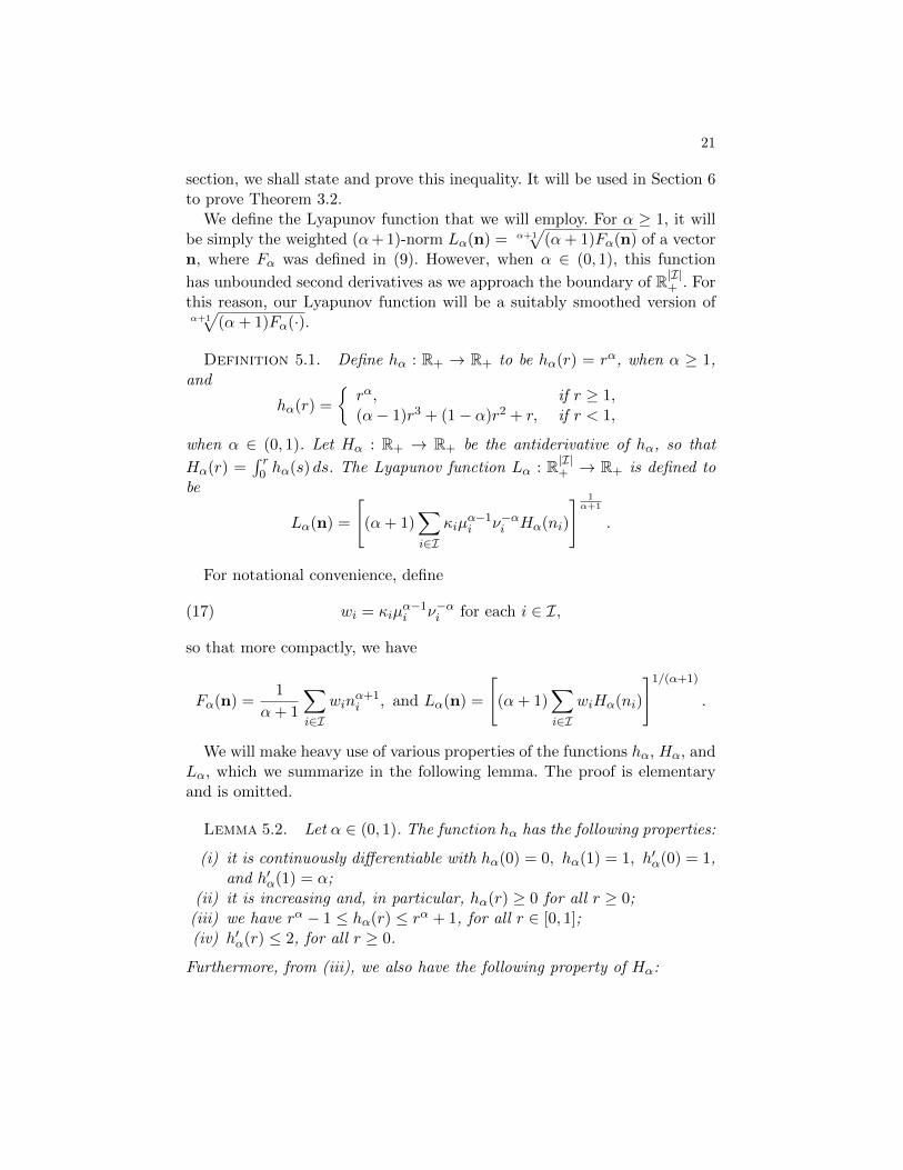
section, we shall state and prove this inequality. It will be used in Section 6to prove Theorem 3.2.
We define the Lyapunov function that we will employ. For α ≥ 1, it willbe simply the weighted (α+ 1)-norm Lα(n) = α+1
√(α+ 1)Fα(n) of a vector
n, where Fα was defined in (9). However, when α ∈ (0, 1), this function
has unbounded second derivatives as we approach the boundary of R|I|+ . Forthis reason, our Lyapunov function will be a suitably smoothed version ofα+1√
(α+ 1)Fα(·).
Definition 5.1. Define hα : R+ → R+ to be hα(r) = rα, when α ≥ 1,and
hα(r) =
rα, if r ≥ 1,(α− 1)r3 + (1− α)r2 + r, if r < 1,
when α ∈ (0, 1). Let Hα : R+ → R+ be the antiderivative of hα, so that
Hα(r) =∫ r0 hα(s) ds. The Lyapunov function Lα : R|I|+ → R+ is defined to
be
Lα(n) =
[(α+ 1)
∑i∈I
κiµα−1i ν−αi Hα(ni)
] 1α+1
.
For notational convenience, define
(17) wi = κiµα−1i ν−αi for each i ∈ I,
so that more compactly, we have
Fα(n) =1
α+ 1
∑i∈I
winα+1i , and Lα(n) =
[(α+ 1)
∑i∈I
wiHα(ni)
]1/(α+1)
.
We will make heavy use of various properties of the functions hα, Hα, andLα, which we summarize in the following lemma. The proof is elementaryand is omitted.
Lemma 5.2. Let α ∈ (0, 1). The function hα has the following properties:
(i) it is continuously differentiable with hα(0) = 0, hα(1) = 1, h′α(0) = 1,and h′α(1) = α;
(ii) it is increasing and, in particular, hα(r) ≥ 0 for all r ≥ 0;(iii) we have rα − 1 ≤ hα(r) ≤ rα + 1, for all r ∈ [0, 1];(iv) h′α(r) ≤ 2, for all r ≥ 0.
Furthermore, from (iii), we also have the following property of Hα:
22 SHAH & TSITSIKLIS & ZHONG
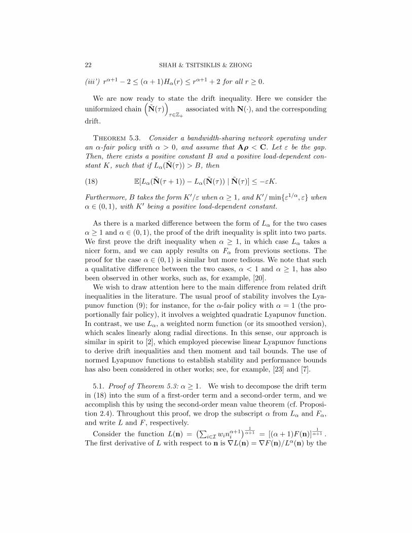
(iii’) rα+1 − 2 ≤ (α+ 1)Hα(r) ≤ rα+1 + 2 for all r ≥ 0.
We are now ready to state the drift inequality. Here we consider the
uniformized chain(N(τ)
)τ∈Z+
associated with N(·), and the corresponding
drift.
Theorem 5.3. Consider a bandwidth-sharing network operating underan α-fair policy with α > 0, and assume that Aρ < C. Let ε be the gap.Then, there exists a positive constant B and a positive load-dependent con-stant K, such that if Lα(N(τ)) > B, then
(18) E[Lα(N(τ + 1))− Lα(N(τ)) | N(τ)] ≤ −εK.
Furthermore, B takes the form K ′/ε when α ≥ 1, and K ′/minε1/α, ε whenα ∈ (0, 1), with K ′ being a positive load-dependent constant.
As there is a marked difference between the form of Lα for the two casesα ≥ 1 and α ∈ (0, 1), the proof of the drift inequality is split into two parts.We first prove the drift inequality when α ≥ 1, in which case Lα takes anicer form, and we can apply results on Fα from previous sections. Theproof for the case α ∈ (0, 1) is similar but more tedious. We note that sucha qualitative difference between the two cases, α < 1 and α ≥ 1, has alsobeen observed in other works, such as, for example, [20].
We wish to draw attention here to the main difference from related driftinequalities in the literature. The usual proof of stability involves the Lya-punov function (9); for instance, for the α-fair policy with α = 1 (the pro-portionally fair policy), it involves a weighted quadratic Lyapunov function.In contrast, we use Lα, a weighted norm function (or its smoothed version),which scales linearly along radial directions. In this sense, our approach issimilar in spirit to [2], which employed piecewise linear Lyapunov functionsto derive drift inequalities and then moment and tail bounds. The use ofnormed Lyapunov functions to establish stability and performance boundshas also been considered in other works; see, for example, [23] and [7].
5.1. Proof of Theorem 5.3: α ≥ 1. We wish to decompose the drift termin (18) into the sum of a first-order term and a second-order term, and weaccomplish this by using the second-order mean value theorem (cf. Proposi-tion 2.4). Throughout this proof, we drop the subscript α from Lα and Fα,and write L and F , respectively.
Consider the function L(n) =(∑
i∈I winα+1i
) 1α+1 = [(α+ 1)F (n)]
1α+1 .
The first derivative of L with respect to n is ∇L(n) = ∇F (n)/Lα(n) by the
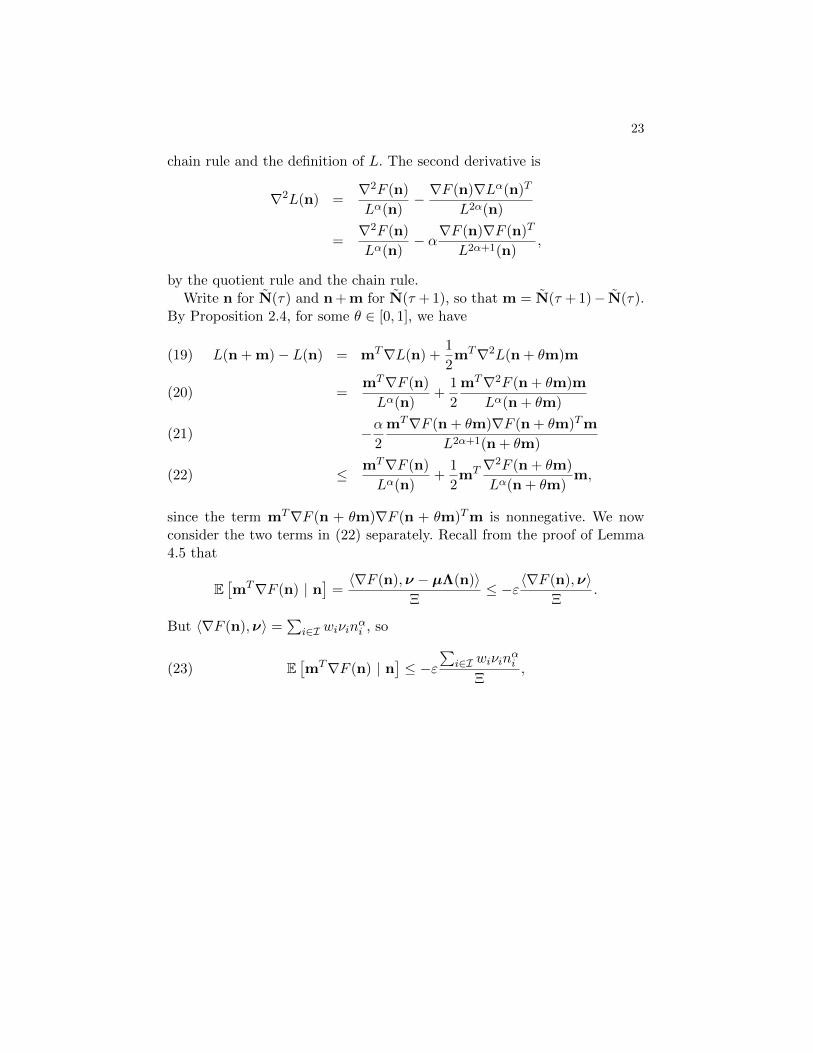
23
chain rule and the definition of L. The second derivative is
∇2L(n) =∇2F (n)
Lα(n)− ∇F (n)∇Lα(n)T
L2α(n)
=∇2F (n)
Lα(n)− α∇F (n)∇F (n)T
L2α+1(n),
by the quotient rule and the chain rule.Write n for N(τ) and n + m for N(τ + 1), so that m = N(τ + 1)− N(τ).
By Proposition 2.4, for some θ ∈ [0, 1], we have
L(n + m)− L(n) = mT∇L(n) +1
2mT∇2L(n + θm)m(19)
=mT∇F (n)
Lα(n)+
1
2
mT∇2F (n + θm)m
Lα(n + θm)(20)
−α2
mT∇F (n + θm)∇F (n + θm)Tm
L2α+1(n + θm)(21)
≤ mT∇F (n)
Lα(n)+
1
2mT ∇2F (n + θm)
Lα(n + θm)m,(22)
since the term mT∇F (n + θm)∇F (n + θm)Tm is nonnegative. We nowconsider the two terms in (22) separately. Recall from the proof of Lemma4.5 that
E[mT∇F (n) | n
]=〈∇F (n),ν − µΛ(n)〉
Ξ≤ −ε〈∇F (n),ν〉
Ξ.
But 〈∇F (n),ν〉 =∑
i∈I wiνinαi , so
(23) E[mT∇F (n) | n
]≤ −ε
∑i∈I wiνin
αi
Ξ,
24 SHAH & TSITSIKLIS & ZHONG
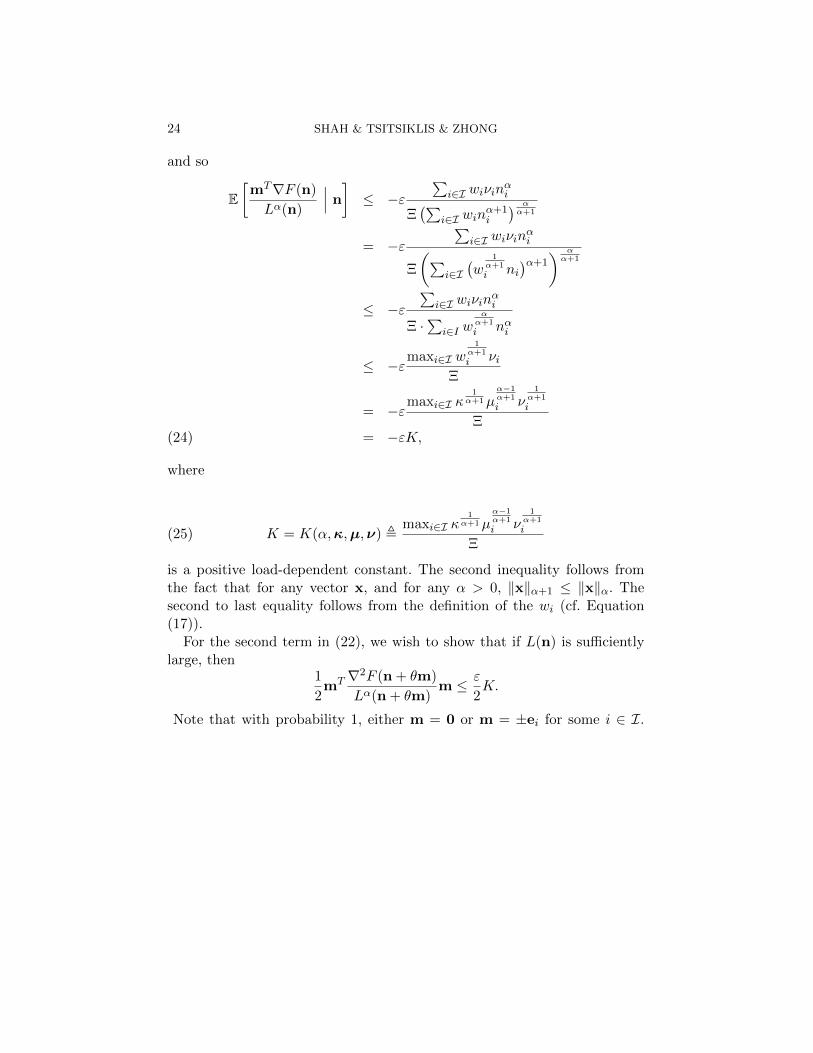
and so
E[mT∇F (n)
Lα(n)
∣∣∣ n
]≤ −ε
∑i∈I wiνin
αi
Ξ(∑
i∈I winα+1i
) αα+1
= −ε∑
i∈I wiνinαi
Ξ
(∑i∈I(w
1α+1
i ni)α+1
) αα+1
≤ −ε∑
i∈I wiνinαi
Ξ ·∑
i∈I wαα+1
i nαi
≤ −εmaxi∈I w
1α+1
i νiΞ
= −εmaxi∈I κ
1α+1µ
α−1α+1
i ν1
α+1
i
Ξ= −εK,(24)
where
(25) K = K(α,κ,µ,ν) ,maxi∈I κ
1α+1µ
α−1α+1
i ν1
α+1
i
Ξ
is a positive load-dependent constant. The second inequality follows fromthe fact that for any vector x, and for any α > 0, ‖x‖α+1 ≤ ‖x‖α. Thesecond to last equality follows from the definition of the wi (cf. Equation(17)).
For the second term in (22), we wish to show that if L(n) is sufficientlylarge, then
1
2mT ∇2F (n + θm)
Lα(n + θm)m ≤ ε
2K.
Note that with probability 1, either m = 0 or m = ±ei for some i ∈ I.
25
Thus
1
2mT ∇2F (n + θm)
Lα(n + θm)m ≤ 1
2
maxi∈I[∇2F (n + θm)
]ii
Lα(n + θm)
=α
2
maxi∈I wi(ni + θmi)α−1[∑
i∈I wi(ni + θmi)α+1] αα+1
≤ α
2
maxi∈I wi(ni + θmi)α−1
wαα+1
i0(ni0 + θmi0)α
≤ α
2w
1α+1
i0(ni0 + θmi0)−1
≤ α
2maxi∈I
w1
α+1
i (ni0 + θmi0)−1,
where i0 ∈ I is such that wi0(ni0 + θmi0)α−1 = maxi∈I wi(ni + θmi)α−1.
Now note that
α
2maxi∈I
w1
α+1
i (ni0 + θmi0)−1 ≤ ε
2K
(where K is defined in (25)) if and only if
ni0 + θmi0 ≥αmaxi∈I w
1α+1
i
K· 1
ε,
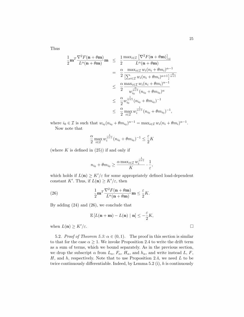
which holds if L(n) ≥ K ′/ε for some appropriately defined load-dependentconstant K ′. Thus, if L(n) ≥ K ′/ε, then
(26)1
2mT ∇2F (n + θm)
Lα(n + θm)m ≤ ε
2K.
By adding (24) and (26), we conclude that
E [L(n + m)− L(n) | n] ≤ −ε2K,
when L(n) ≥ K ′/ε.
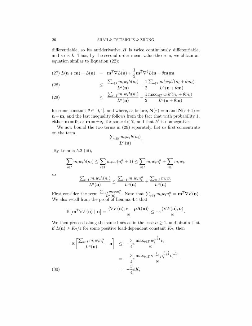
5.2. Proof of Theorem 5.3: α ∈ (0, 1). The proof in this section is similarto that for the case α ≥ 1. We invoke Proposition 2.4 to write the drift termas a sum of terms, which we bound separately. As in the previous section,we drop the subscript α from Lα, Fα, Hα, and hα, and write instead L, F ,H, and h, respectively. Note that to use Proposition 2.4, we need L to betwice continuously differentiable. Indeed, by Lemma 5.2 (i), h is continuously
26 SHAH & TSITSIKLIS & ZHONG
differentiable, so its antiderivative H is twice continuously differentiable,and so is L. Thus, by the second order mean value theorem, we obtain anequation similar to Equation (22):
L(n + m)− L(n) = mT∇L(n) +1
2mT∇2L(n + θm)m(27)
≤∑
i∈I miwih(ni)
Lα(n)+
1
2
∑i∈Im
2iwih
′(ni + θmi)
Lα(n + θm)(28)
≤∑
i∈I miwih(ni)
Lα(n)+
1
2
maxi∈I wih′(ni + θmi)
Lα(n + θm)(29)
for some constant θ ∈ [0, 1], and where, as before, N(τ) = n and N(τ +1) =n + m, and the last inequality follows from the fact that with probability 1,either m = 0, or m = ±ei, for some i ∈ I, and that h′ is nonnegative.
We now bound the two terms in (29) separately. Let us first concentrateon the term ∑
i∈I miwih(ni)
Lα(n).
By Lemma 5.2 (iii),∑i∈I
miwih(ni) ≤∑i∈I
miwi(nαi + 1) ≤
∑i∈I
miwinαi +
∑i∈I
miwi,
so ∑i∈I miwih(ni)
Lα(n)≤∑
i∈I miwinαi
Lα(n)+
∑i∈I miwi
Lα(n).
First consider the term∑i∈I miwin
αi
Lα(n) . Note that∑
i∈I miwinαi = mT∇F (n).
We also recall from the proof of Lemma 4.4 that
E[mT∇F (n) | n
]=〈∇F (n),ν − µΛ(n)〉
Ξ≤ −ε〈∇F (n),ν〉
Ξ.
We then proceed along the same lines as in the case α ≥ 1, and obtain thatif L(n) ≥ K2/ε for some positive load-dependent constant K2, then
E[∑
i∈I miwinαi
Lα(n)
∣∣∣ n
]≤ −3
4ε
maxi∈I w1
α+1
i νiΞ
= −3
4ε
maxi∈I κ1
α+1µα−1α+1
i ν1
α+1
i
Ξ
= −3
4εK,(30)
27
Here as in the proof for the case α ≥ 1,K = K(α,κ,µ,ν) ,maxi∈I κ
1α+1 µ
α−1α+1i ν
1α+1i∑
i∈I νi
is a positive load-dependent constant.
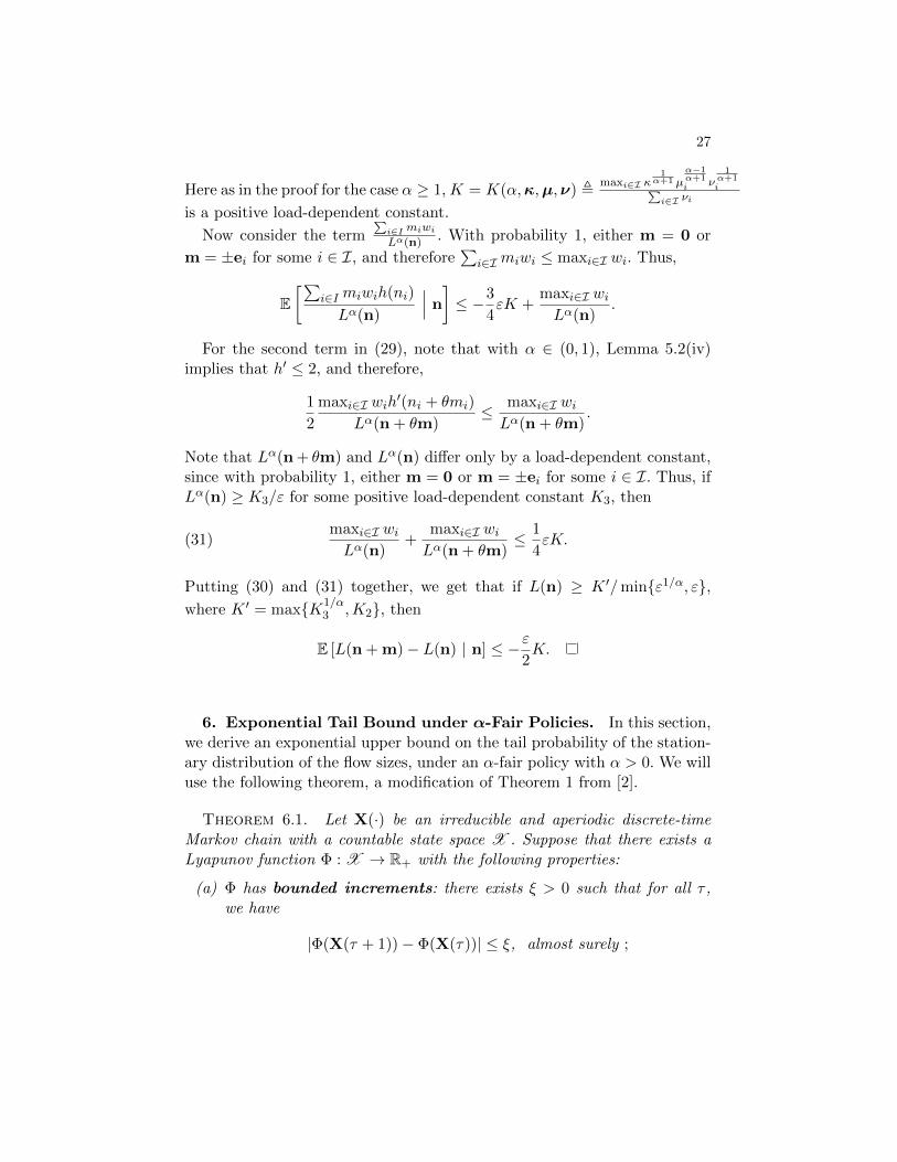
Now consider the term∑i∈I miwiLα(n) . With probability 1, either m = 0 or
m = ±ei for some i ∈ I, and therefore∑
i∈Imiwi ≤ maxi∈I wi. Thus,
E[∑
i∈I miwih(ni)
Lα(n)
∣∣∣ n
]≤ −3
4εK +
maxi∈I wiLα(n)
.
For the second term in (29), note that with α ∈ (0, 1), Lemma 5.2(iv)implies that h′ ≤ 2, and therefore,
1
2
maxi∈I wih′(ni + θmi)
Lα(n + θm)≤ maxi∈I wiLα(n + θm)
.
Note that Lα(n + θm) and Lα(n) differ only by a load-dependent constant,since with probability 1, either m = 0 or m = ±ei for some i ∈ I. Thus, ifLα(n) ≥ K3/ε for some positive load-dependent constant K3, then
(31)maxi∈I wiLα(n)
+maxi∈I wiLα(n + θm)
≤ 1
4εK.
Putting (30) and (31) together, we get that if L(n) ≥ K ′/minε1/α, ε,where K ′ = maxK1/α
3 ,K2, then
E [L(n + m)− L(n) | n] ≤ −ε2K.
6. Exponential Tail Bound under α-Fair Policies. In this section,we derive an exponential upper bound on the tail probability of the station-ary distribution of the flow sizes, under an α-fair policy with α > 0. We willuse the following theorem, a modification of Theorem 1 from [2].
Theorem 6.1. Let X(·) be an irreducible and aperiodic discrete-timeMarkov chain with a countable state space X . Suppose that there exists aLyapunov function Φ : X → R+ with the following properties:
(a) Φ has bounded increments: there exists ξ > 0 such that for all τ ,we have
|Φ(X(τ + 1))− Φ(X(τ))| ≤ ξ, almost surely ;
28 SHAH & TSITSIKLIS & ZHONG
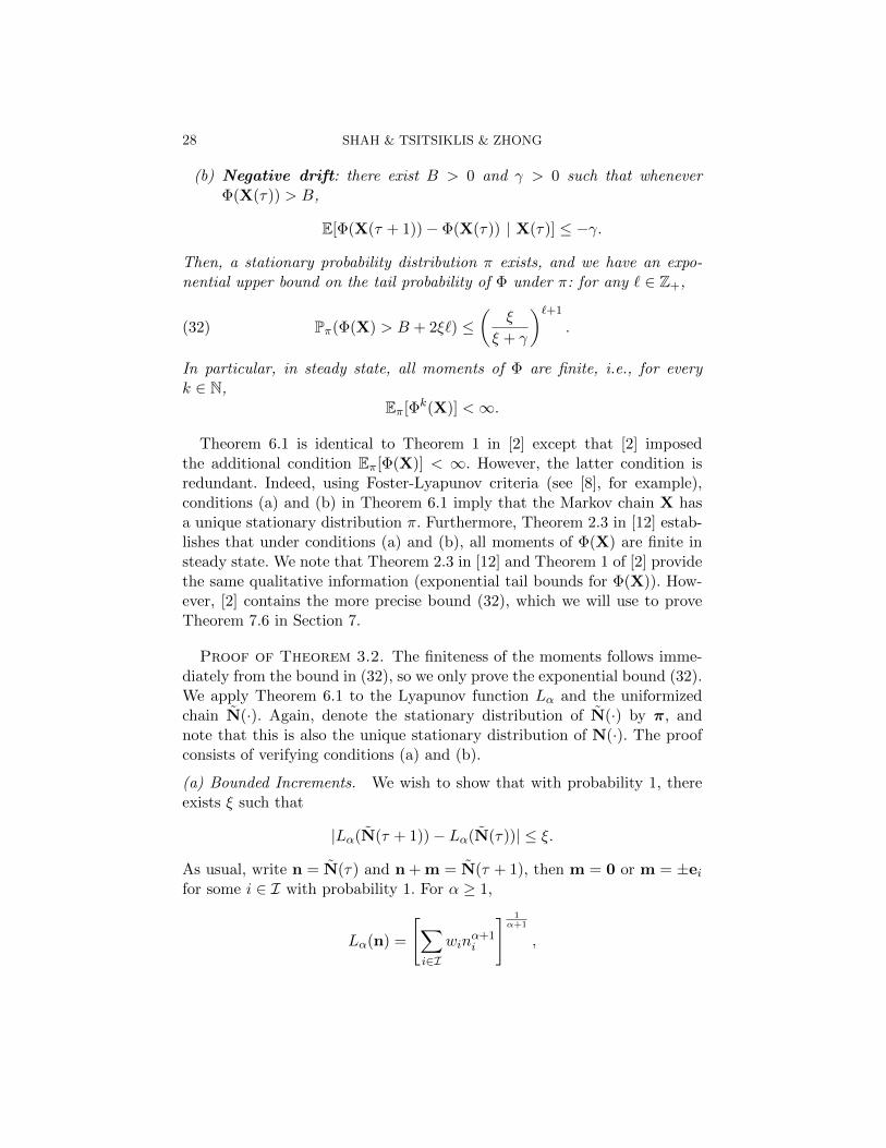
(b) Negative drift: there exist B > 0 and γ > 0 such that wheneverΦ(X(τ)) > B,
E[Φ(X(τ + 1))− Φ(X(τ)) | X(τ)] ≤ −γ.
Then, a stationary probability distribution π exists, and we have an expo-nential upper bound on the tail probability of Φ under π: for any ` ∈ Z+,
(32) Pπ(Φ(X) > B + 2ξ`) ≤(
ξ
ξ + γ
)`+1
.
In particular, in steady state, all moments of Φ are finite, i.e., for everyk ∈ N,
Eπ[Φk(X)] <∞.
Theorem 6.1 is identical to Theorem 1 in [2] except that [2] imposedthe additional condition Eπ[Φ(X)] < ∞. However, the latter condition isredundant. Indeed, using Foster-Lyapunov criteria (see [8], for example),conditions (a) and (b) in Theorem 6.1 imply that the Markov chain X hasa unique stationary distribution π. Furthermore, Theorem 2.3 in [12] estab-lishes that under conditions (a) and (b), all moments of Φ(X) are finite insteady state. We note that Theorem 2.3 in [12] and Theorem 1 of [2] providethe same qualitative information (exponential tail bounds for Φ(X)). How-ever, [2] contains the more precise bound (32), which we will use to proveTheorem 7.6 in Section 7.
Proof of Theorem 3.2. The finiteness of the moments follows imme-diately from the bound in (32), so we only prove the exponential bound (32).We apply Theorem 6.1 to the Lyapunov function Lα and the uniformizedchain N(·). Again, denote the stationary distribution of N(·) by π, andnote that this is also the unique stationary distribution of N(·). The proofconsists of verifying conditions (a) and (b).
(a) Bounded Increments. We wish to show that with probability 1, thereexists ξ such that
|Lα(N(τ + 1))− Lα(N(τ))| ≤ ξ.
As usual, write n = N(τ) and n + m = N(τ + 1), then m = 0 or m = ±eifor some i ∈ I with probability 1. For α ≥ 1,
Lα(n) =
[∑i∈I
winα+1i
] 1α+1
,
29
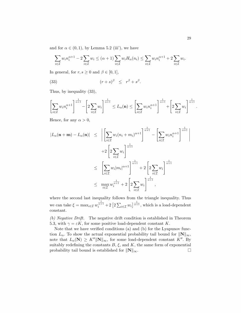
and for α ∈ (0, 1), by Lemma 5.2 (iii’), we have∑i∈I
winα+1i − 2
∑i∈I
wi ≤ (α+ 1)∑i∈I
wiHα(ni) ≤∑i∈I
winα+1i + 2
∑i∈I
wi.
In general, for r, s ≥ 0 and β ∈ [0, 1],
(r + s)β ≤ rβ + sβ.(33)
Thus, by inequality (33),[∑i∈I
winα+1i
] 1α+1
−
[2∑i∈I
wi
] 1α+1
≤ Lα(n) ≤
[∑i∈I
winα+1i
] 1α+1
+
[2∑i∈I
wi
] 1α+1
.
Hence, for any α > 0,
|Lα(n + m)− Lα(n)| ≤
∣∣∣∣∣[∑i∈I
wi(ni +mi)α+1
] 1α+1
−
[∑i∈I
winα+1i
] 1α+1
∣∣∣∣∣+2
[2∑i∈I
wi
] 1α+1
≤
[∑i∈I
wi|mi|α+1
] 1α+1
+ 2
[2∑i∈I
wi
] 1α+1
≤ maxi∈I
w1
α+1
i + 2
[2∑i∈I
wi
] 1α+1
,
where the second last inequality follows from the triangle inequality. Thus
we can take ξ = maxi∈I w1
α+1
i +2[2∑
i∈I wi] 1α+1 , which is a load-dependent
constant.
(b) Negative Drift. The negative drift condition is established in Theorem5.3, with γ = εK, for some positive load-dependent constant K.
Note that we have verified conditions (a) and (b) for the Lyapunov func-tion Lα. To show the actual exponential probability tail bound for ‖N‖∞,note that Lα(N) ≥ K ′′‖N‖∞, for some load-dependent constant K ′′. Bysuitably redefining the constants B, ξ, and K, the same form of exponentialprobability tail bound is established for ‖N‖∞.
30 SHAH & TSITSIKLIS & ZHONG
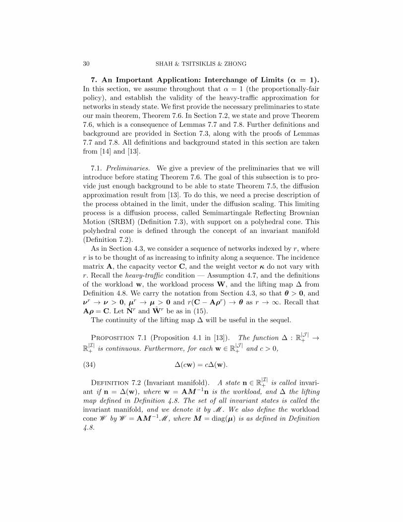
7. An Important Application: Interchange of Limits (α = 1).In this section, we assume throughout that α = 1 (the proportionally-fairpolicy), and establish the validity of the heavy-traffic approximation fornetworks in steady state. We first provide the necessary preliminaries to stateour main theorem, Theorem 7.6. In Section 7.2, we state and prove Theorem7.6, which is a consequence of Lemmas 7.7 and 7.8. Further definitions andbackground are provided in Section 7.3, along with the proofs of Lemmas7.7 and 7.8. All definitions and background stated in this section are takenfrom [14] and [13].
7.1. Preliminaries. We give a preview of the preliminaries that we willintroduce before stating Theorem 7.6. The goal of this subsection is to pro-vide just enough background to be able to state Theorem 7.5, the diffusionapproximation result from [13]. To do this, we need a precise description ofthe process obtained in the limit, under the diffusion scaling. This limitingprocess is a diffusion process, called Semimartingale Reflecting BrownianMotion (SRBM) (Definition 7.3), with support on a polyhedral cone. Thispolyhedral cone is defined through the concept of an invariant manifold(Definition 7.2).
As in Section 4.3, we consider a sequence of networks indexed by r, wherer is to be thought of as increasing to infinity along a sequence. The incidencematrix A, the capacity vector C, and the weight vector κ do not vary withr. Recall the heavy-traffic condition — Assumption 4.7, and the definitionsof the workload w, the workload process W, and the lifting map ∆ fromDefinition 4.8. We carry the notation from Section 4.3, so that θ > 0, andνr → ν > 0, µr → µ > 0 and r(C − Aρr) → θ as r → ∞. Recall thatAρ = C. Let Nr and Wr be as in (15).
The continuity of the lifting map ∆ will be useful in the sequel.
Proposition 7.1 (Proposition 4.1 in [13]). The function ∆ : R|J |+ →R|I|+ is continuous. Furthermore, for each w ∈ R|J |+ and c > 0,
(34) ∆(cw) = c∆(w).
Definition 7.2 (Invariant manifold). A state n ∈ R|I|+ is called invari-ant if n = ∆(w), where w = AM−1n is the workload, and ∆ the liftingmap defined in Definition 4.8. The set of all invariant states is called theinvariant manifold, and we denote it by M . We also define the workloadcone W by W = AM−1M , where M = diag(µ) is as defined in Definition4.8.
31
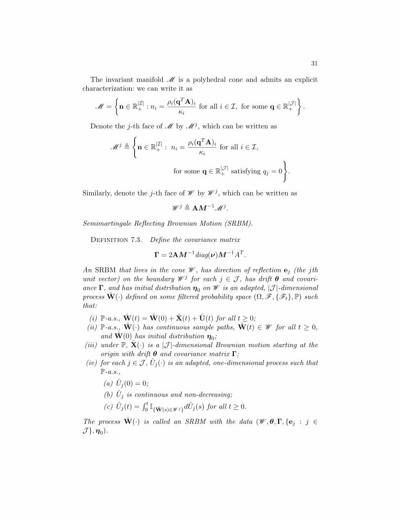
The invariant manifold M is a polyhedral cone and admits an explicitcharacterization: we can write it as
M =
n ∈ R|I|+ : ni =
ρi(qTA)iκi
for all i ∈ I, for some q ∈ R|J |+
.
Denote the j-th face of M by M j , which can be written as
M j ,
n ∈ R|I|+ : ni =
ρi(qTA)iκi
for all i ∈ I,
for some q ∈ R|J |+ satisfying qj = 0
.
Similarly, denote the j-th face of W by W j , which can be written as
W j , AM−1M j .
Semimartingale Reflecting Brownian Motion (SRBM).
Definition 7.3. Define the covariance matrix
Γ = 2AM−1diag(ν)M−1AT .
An SRBM that lives in the cone W , has direction of reflection ej (the jthunit vector) on the boundary W j for each j ∈ J , has drift θ and covari-ance Γ, and has initial distribution η0 on W is an adapted, |J |-dimensionalprocess W(·) defined on some filtered probability space (Ω,F , Ft,P) suchthat:
(i) P-a.s., W(t) = W(0) + X(t) + U(t) for all t ≥ 0;(ii) P-a.s., W(·) has continuous sample paths, W(t) ∈ W for all t ≥ 0,
and W(0) has initial distribution η0;(iii) under P, X(·) is a |J |-dimensional Brownian motion starting at the
origin with drift θ and covariance matrix Γ;(iv) for each j ∈ J , Uj(·) is an adapted, one-dimensional process such that
P-a.s.,
(a) Uj(0) = 0;
(b) Uj is continuous and non-decreasing;
(c) Uj(t) =∫ t0 IW(s)∈W jdUj(s) for all t ≥ 0.
The process W(·) is called an SRBM with the data (W ,θ,Γ, ej : j ∈J ,η0).
32 SHAH & TSITSIKLIS & ZHONG
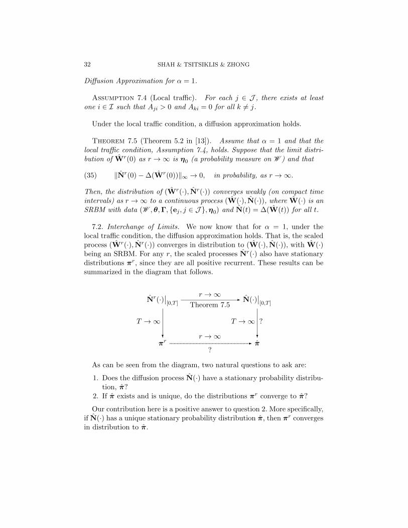
Diffusion Approximation for α = 1.
Assumption 7.4 (Local traffic). For each j ∈ J , there exists at leastone i ∈ I such that Aji > 0 and Aki = 0 for all k 6= j.
Under the local traffic condition, a diffusion approximation holds.
Theorem 7.5 (Theorem 5.2 in [13]). Assume that α = 1 and that thelocal traffic condition, Assumption 7.4, holds. Suppose that the limit distri-bution of Wr(0) as r →∞ is η0 (a probability measure on W ) and that
(35) ‖Nr(0)−∆(Wr(0))‖∞ → 0, in probability, as r →∞.
Then, the distribution of (Wr(·), Nr(·)) converges weakly (on compact timeintervals) as r →∞ to a continuous process (W(·), N(·)), where W(·) is anSRBM with data (W ,θ,Γ, ej , j ∈ J ,η0) and N(t) = ∆(W(t)) for all t.
7.2. Interchange of Limits. We now know that for α = 1, under thelocal traffic condition, the diffusion approximation holds. That is, the scaledprocess (Wr(·), Nr(·)) converges in distribution to (W(·), N(·)), with W(·)being an SRBM. For any r, the scaled processes Nr(·) also have stationarydistributions πr, since they are all positive recurrent. These results can besummarized in the diagram that follows.
Nr(·)∣∣[0,T ]
r →∞Theorem 7.5
- N(·)∣∣[0,T ]
πr
T →∞
?.......................................................
r →∞
?- π
T →∞ ?
?
As can be seen from the diagram, two natural questions to ask are:
1. Does the diffusion process N(·) have a stationary probability distribu-tion, π?
2. If π exists and is unique, do the distributions πr converge to π?
Our contribution here is a positive answer to question 2. More specifically,if N(·) has a unique stationary probability distribution π, then πr convergesin distribution to π.
33
Theorem 7.6. Suppose that α = 1 and that the local traffic condition,Assumption 7.4, holds. Suppose further that N(·) has a unique stationaryprobability distribution π. For each r, let πr be the unique stationary prob-ability distribution of Nr. Then,
πr → π, in distribution, as r →∞.
The line of proof of Theorem 7.6 is fairly standard. We first establishtightness of the set of distributions πr in Lemma 7.7. Letting the pro-cesses Nr(·) be initially distributed as πr, we translate this tightness con-dition into an initial condition similar to (35), in Lemma 7.8. We then applyTheorem 7.5 to deduce the convergence of the processes Nr(·), which by sta-tionarity, leads to the convergence of the distributions πr. We state Lemmas7.7 and 7.8 below, and defer their proofs to the next section.
Lemma 7.7. Suppose that α = 1. The set of probability distributionsπr is tight.
Lemma 7.8. Consider the stationary probability distributions πr of Nr(·),and let πrk be any convergent subsequence of πr. Let Nr(0) be dis-tributed as πr for each r. Then there exists a subsequence r` of rk suchthat
(36)∥∥∥Nr`(0)−∆
(Wr`(0)
)∥∥∥∞→ 0
in probability as ` → ∞, i.e., such that condition (35) holds for the subse-quence (Wr`(·), Nr`(·)).
Proof of Theorem 7.6. Since πr is tight by Lemma 7.7, Prohorov’s theo-rem implies that πr is relatively compact in the weak topology. Let πrkbe a convergent subsequence of the set of probability distributions πr,and suppose that πrk → π as k →∞, in distribution.
Let Nr(0) be distributed as πr for each r. Then by Lemma 7.8, thereexists a subsequence r` of rk such that∥∥∥Nr`(0)−∆
(Wr`(0)
)∥∥∥∞→ 0
in probability as ` → ∞. Denote the distribution of Wr(0) by ηr. Sinceπrk → π as k →∞, πr` → π as `→∞ as well, and ηr` → η as `→∞, forsome probability distribution η.
We now wish to apply Theorem 7.5 to the sequence Nr`(·). The onlycondition that needs to be verified is that η has support on W . This can be
34 SHAH & TSITSIKLIS & ZHONG
argued as follows. Let N(0) have distribution π, and let W(0) = AM−1N(0)be the corresponding workload. Then Wr`(0) → W(0) in distribution asr → ∞, and W(0) has distribution η. The lifting map ∆ is continuous by
Proposition 7.1, so ∆(Wr`(0)
)→ ∆
(W(0)
)in distribution as r → ∞.
This convergence, together with (36) and the fact that Nr`(0) → N(0) in
distribution, implies that N(0) and ∆(W(0)
)are identically distributed.
Now ∆(W(0)
)has support on M , so N(0) is supported on M as well, and
so W(0), hence η, is supported on W .By Theorem 7.5, (Wr`(·), Nr`(·)) converges in distribution to a continuous
process (W(·), N(·)). Suppose that W(·) and N(·) have unique stationarydistributions η and π, respectively. The processes (Wr`(·), Nr`(·)) are sta-tionary, so (W(·), N(·)) is stationary as well. Therefore, W(0) and N(0) aredistributed as η and π, respectively. Since (Wr`(0), Nr`(0))→ (W(0), N(0))in distribution, we have that ηr` → η and πr` → π weakly as `→∞. Thisshows that π = π and η = η. Since πrk is an arbitrary convergent sub-sequence, π is the unique weak limit point of πr, and this shows thatπr → π in distribution.
For Theorem 7.6 to apply, we need to verify that N(·) (or equivalently,W(·)) has a unique stationary distribution. The following theorem statesthat when κi = 1 for all i ∈ I, this condition holds; more specifically, theSRBM W(·) has a unique stationary distribution, which turns out to havea product form.
Theorem 7.9 (Theorem 5.3 in [13]). Suppose that α = 1 and κi = 1for all i ∈ I. Let η be the measure on W that is absolutely continuous withrespect to Lebesgue measure with density given by
(37) p(w) = exp(〈v,w〉), w ∈ W ,
where
(38) v = 2Γ−1θ.
The product measure η is an invariant measure for the SRBM with statespace W , directions of reflection ej , j ∈ J , drift θ, and covariance matrixΓ. After normalization, it defines the unique stationary distribution for theSRBM.
By Theorems 7.6 and 7.9, the following corollary is immediate.
35
Corollary 7.10. Suppose that α = 1 and κi = 1 for all i ∈ I. Supposefurther that the local traffic condition, Assumption 7.4, holds. Let π be theunique stationary probability distribution of N(·). For each r, let πr be theunique stationary probability distribution of Nr. Then,
πr → π, in distribution, as r →∞.
7.3. Proof of Lemmas 7.7 and 7.8.
Proof of Lemma 7.7. To establish tightness, it suffices to show that for
every y > 0 there exists a compact set Ky ⊂ R|I|+ such that
(39) lim supr→∞
πr(R|I|+ \Ky
)≤ e−y.
We now proceed to define the compact sets Ky. As in the proof of Theorem4.10, let εr = ε(ρr) be the gap in the rth system. Then, under Assumption4.7, for sufficiently large r, εr ≥ D/r for some network-dependent constantD > 0. Since α = 1, Theorem 3.2 implies that for the rth system, there existload-dependent constants Kr > 0 and ξr > 0 such that for every ` ∈ Z+,
(40) Pπr
(‖Nr‖∞ ≥
Kr
εr+ 2ξr`
)≤(
ξrξr + εr
)`+1
.
By the definition of a positive load-dependent constant, there exist contin-uous functions f1 and f2 on the open positive orthant such that for all r,Kr = f1(µ
r,νr) and ξr = f2(µr,νr). Since µr → µ > 0 and νr → ν > 0,
we have Kr → K , f1(µ,ν) > 0 and ξr → ξ , f2(µ,ν) > 0. Define
Ky ,
v ∈ R|I|+ : ‖v‖∞ ≤
(K + 1) + 4(ξ + 1)2 · yD
.
We now show that (39) holds, or equivalently, by the definition of Ky, weshow that for every y > 0,
(41) lim supr→∞
Pπr
(1
r‖Nr‖∞ >
(K + 1) + 4(ξ + 1)2y
D
)≤ e−y.
Let `r , b2ξry/εrc, where for z ∈ R, bzc is the largest integer not exceedingz. By (40), we have
Pπr
(1
r‖Nr‖∞ ≥
Kr
rεr+
2ξr`rr
)≤
(1
1 + εrξr
)`r+1
.
36 SHAH & TSITSIKLIS & ZHONG
Taking logarithms on both sides, we have
logPπr
(1
r‖Nr‖∞ ≥
Kr
rεr+
2ξr`rr
)≤ −(`r + 1) log
(1 +
εrξr
).
Since εr → 0 and ξr → ξ > 0 as r →∞, εrξr < 1 for sufficiently large r. Sincelog(1 + t) ≥ t/2 for t ∈ [0, 1], we have
−(`r + 1) log
(1 +
εrξr
)≤ −(`r + 1)
εr2ξr
,
when r is sufficiently large. By definition, `r = b2ξry/εrc, so `r+1 ≥ 2ξrx/εr,or equivalently, −(`r + 1) εr2ξr ≤ −y. Thus, when r is sufficiently large,
logPπr
(1
r‖Nr‖∞ ≥
Kr
rεr+
2ξr`rr
)≤ −y.
Consider the term Krrεr
+ 2ξr`rr . When r is sufficiently large, rεr ≥ D, Kr ≤
K + 1, and ξr ≤ ξ + 1, and so
Kr
rεr+
2ξr`rr≤ Kr
rεr+
2ξr(2ξry)
rεr≤ K + 1
D+
4(ξ + 1)2y
D.
Thus, for sufficiently large r,
logPπr
(1
r‖Nr‖∞ >
(K + 1) + 4(ξ + 1)2y
D
)≤ logPπr
(1
r‖Nr‖∞ ≥
Kr
rεr+
2ξr`rr
)≤ −y.
This establishes (41), and also the tightness of πr.
Next, we prove Lemma 7.8. To this end, we need some definitions andbackground. In particular, we need the concept and properties of fluid modelsolutions.
Definition 7.11. A fluid model solution (FMS) is an absolutely con-
tinuous function n : [0,∞)→ R|I|+ such that at each regular point 1 t > 0 ofn(·), we have, for each i ∈ I,
(42)d
dtni(t) =
νi − µiΛi(n(t)), if ni(t) > 0,0, if ni(t) = 0,
1A point t ∈ (0,∞) is a regular point of an absolutely continuous function f : [0,∞)→R|I|+ if each component of f is differentiable at t. Since n is absolutely continuous, almostevery time t ∈ (0,∞) is a regular point for n.
37
and for each j ∈ J ,
(43)∑
i∈I+(n(t))
AjiΛi(n(t)) +∑
i∈I0(n(t))
Ajiρi ≤ Cj ,
where I+(n(t)) = i ∈ I : ni(t) > 0 and I0(n(t)) = i ∈ I : ni(t) = 0.Note that here Aρ = C.
We now collect some properties of a FMS. The following proposition statesthat the invariant manifold M consists exactly of the stationary points of aFMS.
Proposition 7.12 (Theorem 4.1 in [13]). A vector n0 is an invariantstate, that is, n0 ∈M , if and only if for every fluid model solution n(·) withn(0) = n0, we have n(t) = n0 for all t > 0.
The following theorem states that starting from any initial condition, aFMS will eventually be close to the invariant manifold M .
Theorem 7.13 (Theorem 5.2 in [14]). Fix R ∈ (0,∞) and δ > 0. Thereis a constant TR,δ <∞ such that for every fluid model solution n(·) satisfying‖n(0)‖∞ ≤ R we have
d(n(t),M ) < δ, for all t > TR,δ,
where d(n(t),M ) , infn∈M ‖n − n(t)‖∞ is the distance from n(t) to themanifold M .
Proposition 7.14 states that the value of the Lyapunov function F1 definedin (9) decreases along the path of any FMS.
Proposition 7.14 (Corollary 6.1 in [14]). At any regular point t of afluid model solution n(·), we have
d
dtF1(n(t)) ≤ 0,
and the inequality is strict if n(t) /∈M .
Using Proposition 7.14, and the continuity of the lifting map ∆, we cantranslate Theorem 7.13 into the following version, which will be used toprove Lemma 7.8.
38 SHAH & TSITSIKLIS & ZHONG
Lemma 7.15. Fix R ∈ (0,∞) and δ > 0. There is a constant TR,δ <∞such that for every fluid model solution n(·) satisfying ‖n(0)‖∞ ≤ R we have
‖n(t)−∆(w(t))‖∞ < δ, for all t > TR,δ,
where w(t) = w(n(t)) is the workload corresponding to n(t) (see Definition4.8).
Proof. Fix R > 0 and δ > 0. Let ‖n(0)‖∞ ≤ R. Then,
F1(n(0)) =1
2
∑i∈I
ν−1i κin2i (0) ≤ R′,
where R′ depends on R and the system parameters. Since n(·) is absolutelycontinuous, by Proposition 7.14 and the fundamental theorem of calculus,we have that F1(n(t)) ≤ R′ for all t ≥ 0. Define the set
S , n ∈ R|I|+ : F1(n) ≤ R′,
and its δ-fattening
Sδ , n ∈ R|I|+ : ‖n− n′‖ ≤ δ for some n′ ∈ S.
Note that both S and Sδ are compact sets, and n(t) ∈ S ⊂ Sδ for all t ≥ 0.Now consider the workload w defined in Definition 4.8. Define the set
w(Sδ) = v ∈ R|J |+ : v = w(n) for some n ∈ Sδ. Since w is a linear map,there exists a load-dependent constant H such that
‖w(n)−w(n′)‖∞ ≤ H‖n− n′‖∞,
for any n,n′ ∈ R|I|+ . Thus w(Sδ) is also a compact set. Since n(t) ∈ Sδ forall t ≥ 0, w(t) ∈ w(Sδ) for all t ≥ 0. By Proposition 7.1, ∆ is a continuousmap, so ∆ is uniformly continuous when restricted to w(Sδ). Therefore,there exists δ′ > 0 such that for any w′,w ∈ w(Sδ) with ‖w′ −w‖∞ < δ′,‖∆(w′)−∆(w)‖∞ < δ
2 . Thus for any n,n′ ∈ Sδ with ‖n−n′‖∞ < δ′/H, wehave ‖w(n)−w(n′)‖ ≤ δ′, and
‖∆(w(n))−∆(w(n′))‖∞ <δ
2.
Let δ′′ = minδ/2, δ′/H. By Theorem 7.13, there exists TR,δ′′ such that forall t ≥ TR,δ′′ ,
d(M ,n(t)) < δ′′.
39
In particular, there exists n ∈ M (which may depend on n(t)) such that‖n− n(t)‖∞ < δ′′ < δ′/H. Since n(t) ∈ S and δ′′ < δ, n ∈ Sδ as well. Thus
‖∆(w(n))−∆(w(n(t)))‖∞ <δ
2.
By Proposition 7.12, since n ∈M , we have n = ∆(w(n)), and hence
‖n−∆(w(n(t)))‖∞ <δ
2.
Thus for all t ≥ TR,δ′′ ,
‖n(t)−∆(w(t))‖∞ ≤ ‖n− n(t)‖∞ + ‖n−∆(w(t))‖∞
< δ′′ +δ
2≤ δ
2+δ
2= δ.
Note that δ′′ depends on R, δ, and the system parameters. Thus, we canrewrite TR,δ′′ as TR,δ. This concludes the proof of the lemma.
The last property of a FMS that we need is the tightness of the fluid-scaledprocesses Nr and Wr, defined by
(44) Nr(t) = Nr(rt)/r, and Wr(t) = Wr(rt)/r.
Theorem 7.16 (Theorem B.1 in [14]). Suppose that Nr(0) converges
in distribution as r →∞ to a random variable taking values in R|I|+ . Then,the sequence Nr(·) is C-tight 2, and any weak limit point N(·) of thissequence, almost surely satisfies the fluid model equations (42) and (43).
Proof of Lemma 7.8. Consider the unique stationary distributions πr ofNr(·), and ηr of Wr(·). Let πrk be a convergent subsequence, and supposethat πrk → π in distribution, as k →∞. Suppose that at time 0, 1
rkNrk(0)
is distributed as πrk . Then 1rk
Wrk(0) is distributed as ηrk, which convergesin distribution as well, say to η.
We now use the earlier stated FMS properties to prove the lemma. Notethat for all r,
1
rNr(0) = Nr(0) = Nr(0) and
1
rWr(0) = Wr(0) = Wr(0),
2Consider the space D|I| of functions f : [0,∞) → R|I| that are right-continuous on[0,∞) and have finite limits from the left on (0,∞). Let this space be endowed withthe usual Skorohod topology (cf. Section 12 of [3]). The sequence Nr(·) is tight if theprobability measures induced on D|I| are tight. The sequence is C-tight if it is tight andany weak limit point is a measure supported on the set of continuous sample paths.

40 SHAH & TSITSIKLIS & ZHONG
and consider the fluid-scaled processes Nrk(·) and Wrk(·). SinceNrk(0)
converges in distribution to π, Theorem 7.16 implies that the sequenceNrk(·) is C-tight, and any weak limit N(·) almost surely satisfies the fluidmodel equations. Let N(·) be a weak limit point of
Nrk(·)
, and suppose
that the subsequence Nr`(·) of Nrk(·) converges weakly to N(·).Let δ > 0. We will show that we can find r(δ) such that for r` > r(δ),
P(‖Nr`(0)−∆(Wr`(0))‖∞ > δ
)< δ.
Since N(0) is a well-defined random variable, there exists Rδ > 0 such that
P(‖N(0)‖∞ > Rδ
)<δ
2.
Now, for all sample paths ω such that ‖N(0)(ω)‖∞ ≤ Rδ, and such thatN(·)(ω) satisfies the fluid model equations, Lemma 7.15 implies that thereexists T , TRδ,δ such that
‖N(T )(ω)−∆(W(T ))(ω)‖∞ < δ.
Since N(·) satisfies the fluid model equations almost surely, we have
P(‖N(T )−∆(W(T ))‖∞ < δ) > 1− δ
2.
Now for each r, Nr(0) is distributed according to the stationary distributionπr, so Nr(·) is a stationary process. Since Nr`(·)→ N(·) weakly as `→∞,N is also a stationary process. Thus, N(T ) and N(0) are both distributedaccording to π. This implies that
P(‖N(0)−∆(W(0))‖∞ < δ) > 1− δ
2.
Furthermore, since Nr`(0)→ N(0) in distribution,
P(‖Nr`(0)−∆(Wr`(0))‖∞ < δ)→ P(‖N(0)−∆(W(0))‖∞ < δ)
as `→∞. Thus there exists r(δ) such that for all r` > r(δ),
P(‖Nr`(0)−∆(Wr`(0))‖∞ < δ) > 1− δ.
Since δ > 0 is arbitrary,
‖Nr`(0)−∆(Wr`(0))‖∞ = ‖Nr`(0)−∆(Wr`(0))‖∞ → 0,
in probability.
41
8. Conclusion. The results in this paper can be viewed from two dif-ferent perspectives. On the one hand, they provide much new informationon the qualitative behavior (e.g., finiteness of the expected number of flows,bounds on steady-state tail probabilities and finite-horizon maximum excur-sion probabilities, etc.) of the α-fair policies for bandwidth-sharing networkmodels. At an abstract level, our results highlight the importance of re-lying on a suitable Lyapunov function. Even if a network is shown to bestable by using a particular Lyapunov function, different choices and moredetailed analysis may lead to more powerful bounds. At a more concretelevel, we presented a generic method for deriving full state space collapsefrom multiplicative state space collapse, and another for deriving steady-state exponential tail bounds. The methods and results in this paper can beextended to general switched network models. Parallel results for a packetlevel model are detailed in [18].
REFERENCES
[1] D. Bertsekas. Nonlinear Programming. Athena Scientific, 1999.
[2] D. Bertsimas, D. Gamarnik, and J. N. Tsitsiklis. Performance of multiclass Markovianqueueing networks via piecewise linear Lyapunov functions. The Annals of AppliedProbability, 11(4):1384–1428, 2001.
[3] P. Billingsley. Convergence of Probability Measures. Wiley-Interscience, 1999.
[4] T. Bonald and L. Massoulie. Impact of fairness on Internet performance. ACMSIGMETRICS Performance Evaluation Review, 29(1):82–91, 2001.
[5] M. Bramson. State space collapse with application to heavy traffic limits for multi-class queueing networks. Queueing Systems, 30:89–148, 1998.
[6] G. De Veciana, T. Konstantopoulos, and T. Lee. Stability and performance analysisof networks supporting elastic services. IEEE/ACM Transactions on Networking(TON), 9(1), 2001.
[7] A. Eryilmaz and R. Srikant. Asymptotically tight steady-state queue length boundsimplied by drift conditions. Arxiv, April 2011.
[8] S. Foss and T. Konstantopoulos. An overview of some stochastic stability methods.Journal of Operations Research, Society of Japan, 47(4), 2004.
[9] R. Gallager. Discrete Stochastic Processes. Kluwer Academic Publishers, 1996.
[10] D. Gamarnik and A. Zeevi. Validity of heavy traffic steady-state approximations ingeneralized Jackson networks. The Annals of Applied Probability, 16(1):56 – 90, 2006.
[11] G. Grimmett and D. Stirzaker. Probability and Random Processes. Oxford UniversityPress, 2001.
[12] B. Hajek. Hitting and occupation time bounds implied by drift analysis with appli-cations. Advances of Applied Probability, 14:502–525, 1982.
[13] W. Kang, F. Kelly, N. Lee, and R. Williams. State space collapse and diffusionapproximation for a network operating under a fair bandwidth sharing policy. TheAnnals of Applied Probability, 19(5):1719–1780, 2009.
[14] F. Kelly and R. Williams. Fluid model for a network operating under a fairbandwidth-sharing policy. The Annals of Applied Probability, 14(3):1055–1083, 2004.
42 SHAH & TSITSIKLIS & ZHONG
[15] F. P. Kelly, A. K. Maulloo, and D. K. H. Tan. Rate control for communication net-works: shadow prices, proportional fairness and stability. Journal of the OperationalResearch Society, 49(3):237–252, March 1998.
[16] J. Mo and J. Walrand. Fair end-to-end window-based congestion control. IEEE/ACM Transactions on Networking, 8(5):556–567, 2000.
[17] J. Roberts and L. Massoulie. Bandwidth sharing and admission control for elastictraffic. Telecomunication Systems, 15:185–201, 2000.
[18] D. Shah, J. N. Tsitsiklis, and Y. Zhong. Qualitative properties of alpha-weightedscheduling policies. In Proceedings of the ACM SIGMETRICS, June 2010.
[19] D. Shah and D. J. Wischik. Switched networks with maximum weight policies: Fluidapproximation and multiplicative state space collapse. The Annals of Applied Prob-ability, 22(1):70–127, 2012.
[20] R. Srikant. Models and Methods for analyzing Internet congestion control algorithms.Advances in Communication Control Networks in the series “Lecture Notes in Controland Information Sciences,” 308:416–419, 2005.
[21] A. Stolyar. Large deviations of queues sharing a randomly time-varying server.Queueing Systems, 59(1):1–35, 2008.
[22] V. Subramanian. LDP for max-weight scheduling over convex compact rate-regions,June 2010. Mathematics of Operations Research, 35(4):881–910, 2010.
[23] V. J. Venkataramanan and X. Lin. On the large-deviations optimality of schedulingpolicies minimizing the drift of a Lyapunov function. In Proceedings of the 47thAnnual Allerton Conference on Communication, Control, and Computing, September2009.
[24] R. Williams. Diffusion approximations for open multiclass queueing networks: suffi-cient conditions involving state space collapse. Queueing Systems, 30:27–88, 1998.
[25] H. Ye and D. Yao. A stochastic network under proportional fair resource control -diffusion limit with multiple bottlenecks. To appear in Operations Research.

![AMINO ACIDS [QUALITATIVE TESTS] BCH 302 [PRACTICAL]](https://static.fdocument.org/doc/165x107/56649db35503460f94aa38d5/amino-acids-qualitative-tests-bch-302-practical.jpg)