Properties of optimizations used in penalizedGaussian likelihood inverse covariance matrix

estimation

Adam J. RothmanSchool of Statistics

University of Minnesota

October 8, 2014, joint work with Liliana Forzani

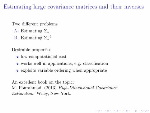
Estimating large covariance matrices and their inverses

Two different problems

A. Estimating Σ∗

B. Estimating Σ−1∗

Desirable properties

low computational cost

works well in applications, e.g. classification

exploits variable ordering when appropriate

An excellent book on the topic:M. Pourahmadi (2013) High-Dimensional CovarianceEstimation. Wiley, New York.

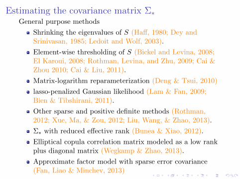
Estimating the covariance matrix Σ∗General purpose methods

Shrinking the eigenvalues of S (Haff, 1980; Dey andSrinivasan, 1985; Ledoit and Wolf, 2003).

Element-wise thresholding of S (Bickel and Levina, 2008;El Karoui, 2008; Rothman, Levina, and Zhu, 2009; Cai &Zhou 2010; Cai & Liu, 2011).

Matrix-logarithm reparameterization (Deng & Tsui, 2010)

lasso-penalized Gaussian likelihood (Lam & Fan, 2009;Bien & Tibshirani, 2011).

Other sparse and positive definite methods (Rothman,2012; Xue, Ma, & Zou, 2012; Liu, Wang, & Zhao, 2013).

Σ∗ with reduced effective rank (Bunea & Xiao, 2012).

Elliptical copula correlation matrix modeled as a low rankplus diagonal matrix (Wegkamp & Zhao, 2013).

Approximate factor model with sparse error covariance(Fan, Liao & Minchev, 2013)

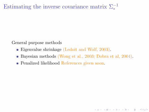
Estimating the inverse covariance matrix Σ−1∗

General purpose methods

Eigenvalue shrinkage (Ledoit and Wolf, 2003).

Bayesian methods (Wong et al., 2003; Dobra et al, 2004).

Penalized likelihood References given soon.

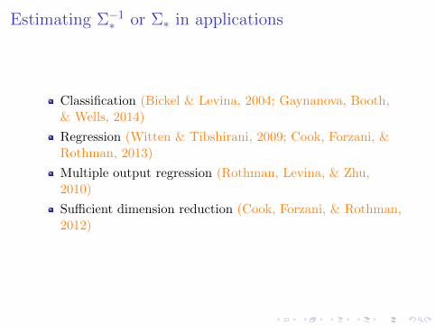
Estimating Σ−1∗ or Σ∗ in applications

Classification (Bickel & Levina, 2004; Gaynanova, Booth,& Wells, 2014)

Regression (Witten & Tibshirani, 2009; Cook, Forzani, &Rothman, 2013)

Multiple output regression (Rothman, Levina, & Zhu,2010)

Sufficient dimension reduction (Cook, Forzani, & Rothman,2012)

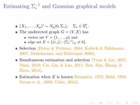
Estimating Σ−1∗ and Gaussian graphical models

(X1, . . . , Xp)′ ∼ Np(0,Σ∗), Σ∗ ∈ Sp+.

The undirected graph G = (V,E) has

vertex set V = 1, . . . , p andedge set E = (i, j) : (Σ−1∗ )ij 6= 0.

Selection (Drton & Perlman, 2004; Kalisch & Buhlmann,2007; Meinshausen and Buhlmann 2006).

Simultaneous estimation and selection (Yuan & Lin, 2007;Yuan, 2010; Cai, Liu, & Luo, 2011; Ren, Sun, Zhang, &Zhou, 2013).

Estimation when E is known Dempster, 1972; Buhl, 1993;Drton et al., 2009; Uhler, 2012).

Part I: On solution existence in penalizedGaussian likelihood estimation of Σ−1

∗

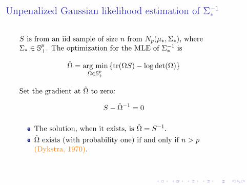
Unpenalized Gaussian likelihood estimation of Σ−1∗

S is from an iid sample of size n from Np(µ∗,Σ∗), whereΣ∗ ∈ Sp+. The optimization for the MLE of Σ−1

∗ is

Ω = arg minΩ∈Sp+

tr(ΩS)− log det(Ω)

Set the gradient at Ω to zero:

S − Ω−1 = 0

The solution, when it exists, is Ω = S−1.

Ω exists (with probability one) if and only if n > p(Dykstra, 1970).

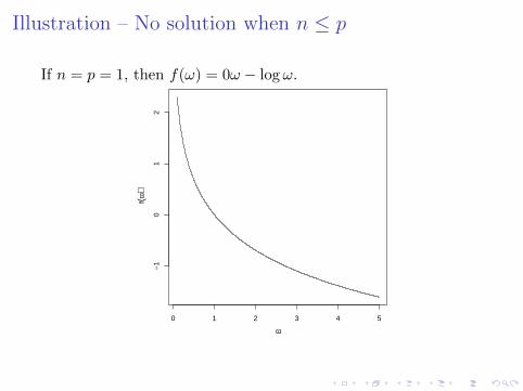
Illustration – No solution when n ≤ p

If n = p = 1, then f(ω) = 0ω − logω.

0 1 2 3 4 5

−1

01

2

ω

f(ω)

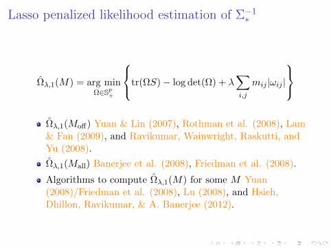
Lasso penalized likelihood estimation of Σ−1∗

Ωλ,1(M) = arg minΩ∈Sp+

tr(ΩS)− log det(Ω) + λ∑i,j

mij |ωij |

Ωλ,1(Moff) Yuan & Lin (2007), Rothman et al. (2008), Lam& Fan (2009), and Ravikumar, Wainwright, Raskutti, andYu (2008).

Ωλ,1(Mall) Banerjee et al. (2008), Friedman et al. (2008).

Algorithms to compute Ωλ,1(M) for some M Yuan(2008)/Friedman et al. (2008), Lu (2008), and Hsieh,Dhillon, Ravikumar, & A. Banerjee (2012).

Review of work on solution existence

Banerjee et al. (2008) showed that a solution exists ifM = Mall and λ > 0.

Ravikumar et al. (2008) showed that a solution exists ifM = Moff , λ > 0, and S I ∈ Sp+.

Lu (2008) showed that a solution exists if S + λM I ∈ Sp+.

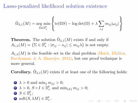
Lasso-penalized likelihood solution existence

Ωλ,1(M) = arg minΩ∈Sp+

tr(ΩS)− log det(Ω) + λ∑i,j

mij |ωij |

Theorem. The solution Ωλ,1(M) exists if and only ifA1,λ(M) = Σ ∈ Sp+ : |σij − sij | ≤ mijλ is not empty.

A1,λ(M) is the feasible set in the dual problem (Hsieh, Dhillon,Ravikumar, & A. Banerjee, 2012), but our proof technique ismore general.

Corollary. Ωλ,1(M) exists if at least one of the following holds:

1 λ > 0 and minjmjj > 0;2 λ > 0, S I ∈ Sp+ and mini 6=jmij > 0;3 S ∈ Sp+;4 soft(S, λM) ∈ Sp+.

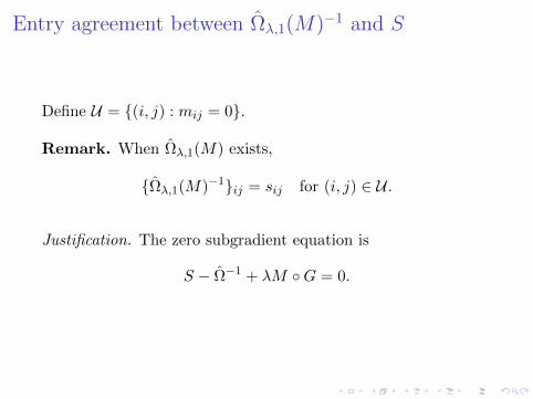
Entry agreement between Ωλ,1(M)−1 and S

Define U = (i, j) : mij = 0.

Remark. When Ωλ,1(M) exists,

Ωλ,1(M)−1ij = sij for (i, j) ∈ U .

Justification. The zero subgradient equation is

S − Ω−1 + λM G = 0.

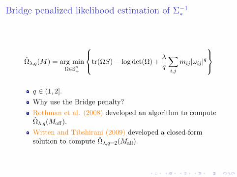
Bridge penalized likelihood estimation of Σ−1∗

Ωλ,q(M) = arg minΩ∈Sp+

tr(ΩS)− log det(Ω) +λ

q

∑i,j

mij |ωij |q

q ∈ (1, 2].

Why use the Bridge penalty?

Rothman et al. (2008) developed an algorithm to computeΩλ,q(Moff).

Witten and Tibshirani (2009) developed a closed-formsolution to compute Ωλ,q=2(Mall).

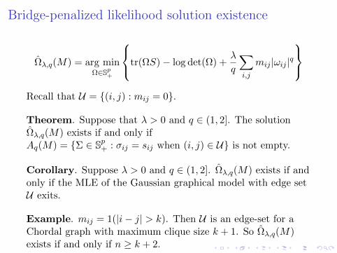
Bridge-penalized likelihood solution existence

Ωλ,q(M) = arg minΩ∈Sp+

tr(ΩS)− log det(Ω) +λ

q

∑i,j

mij |ωij |q

Recall that U = (i, j) : mij = 0.

Theorem. Suppose that λ > 0 and q ∈ (1, 2]. The solutionΩλ,q(M) exists if and only ifAq(M) = Σ ∈ Sp+ : σij = sij when (i, j) ∈ U is not empty.

Corollary. Suppose λ > 0 and q ∈ (1, 2]. Ωλ,q(M) exists if andonly if the MLE of the Gaussian graphical model with edge setU exits.

Example. mij = 1(|i− j| > k). Then U is an edge-set for aChordal graph with maximum clique size k + 1. So Ωλ,q(M)exists if and only if n ≥ k + 2.

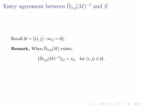
Entry agreement between Ωλ,q(M)−1 and S

Recall U = (i, j) : mij = 0.

Remark. When Ωλ,q(M) exists,

Ωλ,q(M)−1ij = sij for (i, j) ∈ U .

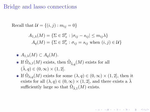
Bridge and lasso connections

Recall that U = (i, j) : mij = 0

A1,λ(M) = Σ ∈ Sp+ : |σij − sij | ≤ mijλAq(M) = Σ ∈ Sp+ : σij = sij when (i, j) ∈ U

A1,λ(M) ⊂ Aq(M).

If Ωλ,1(M) exists, then Ωλ,q(M) exists for all

(λ, q) ∈ (0,∞)× (1, 2].

If Ωλ,q(M) exists for some (λ, q) ∈ (0,∞)× (1, 2], then itexists for all (λ, q) ∈ (0,∞)× (1, 2], and there exists a λsufficiently large so that Ωλ,1(M) exists.

Part II: new algorithm for the ridge penalty

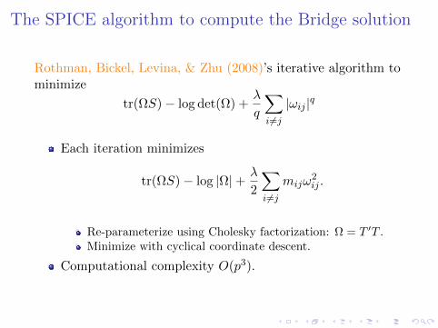
The SPICE algorithm to compute the Bridge solution

Rothman, Bickel, Levina, & Zhu (2008)’s iterative algorithm tominimize

tr(ΩS)− log det(Ω) +λ

q

∑i 6=j|ωij |q

Each iteration minimizes

tr(ΩS)− log |Ω|+ λ

2

∑i 6=j

mijω2ij .

Re-parameterize using Cholesky factorization: Ω = T ′T .Minimize with cyclical coordinate descent.

Computational complexity O(p3).

Accelerated MM algorithm to compute the Ridgesolution (our proposal)

Minimizes the objective function f ,

f(Ω) = tr(ΩS)− log det(Ω) + 0.5λ∑i,j

mijω2ij .

At the kth iteration, the next iterate Ωk+1 is the minimizerof a majorizing function to f at Ωk.

Every few iterations a minorizing function to f at Ωk isminimized. This minimizer is accepted if it improvesobjective function value.

Computational complexity O(p3).

Majorizing f at Ωk part 1

Decompose the penalty:∑i,j

mijω2ij = max

i,jmij

∑i,j

ω2ij −

∑i,j

(maxi,j

mij −mij)ω2ij .

Replace the second term with a linear approximation at ourcurrent iterate Ωk to get the majorizer.

Majorizing f at Ωk part 2

The minimizer of the majorizer to f at Ωk is

Ωk+1 = arg minΩ∈Sp+

tr(ΩS)− log det(Ω) + 0.5λ∑i,j

ω2ij

,

where S = S − λΩk [maxi,jmij −mij ] andλ = λmaxi,jmij .

Closed-form solution derived by Witten and Tibshirani(2009).

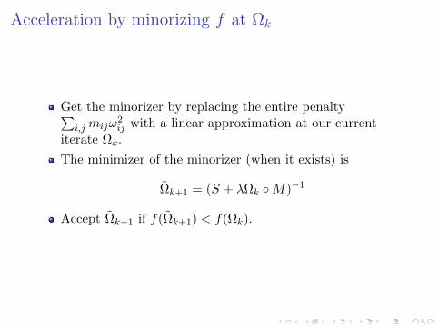
Acceleration by minorizing f at Ωk

Get the minorizer by replacing the entire penalty∑i,jmijω

2ij with a linear approximation at our current

iterate Ωk.

The minimizer of the minorizer (when it exists) is

Ωk+1 = (S + λΩk M)−1

Accept Ωk+1 if f(Ωk+1) < f(Ωk).

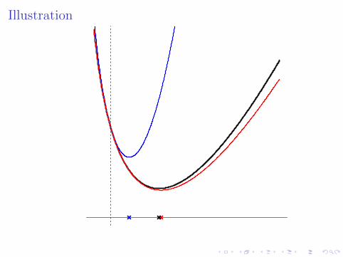
Illustration

Algorithm convergence

Theorem. Suppose that acceleration attempts are stoppedafter a finite number of iterations and the algorithm isinitialized at Ω0 ∈ Sp+. If the global minimizer Ωλ,2(M) exits,then

limk→∞

‖Ωk − Ωλ,2(M)‖ = 0.

Also, if the algorithm converges, then it converges to the globalminimizer.

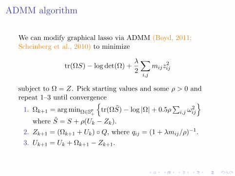
ADMM algorithm

We can modify graphical lasso via ADMM (Boyd, 2011;Scheinberg et al., 2010) to minimize

tr(ΩS)− log det(Ω) +λ

2

∑i,j

mijz2ij

subject to Ω = Z. Pick starting values and some ρ > 0 andrepeat 1–3 until convergence

1. Ωk+1 = arg minΩ∈Sp+

tr(ΩS)− log |Ω|+ 0.5ρ

∑i,j ω

2ij

where S = S + ρ(Uk − Zk).

2. Zk+1 = (Ωk+1 + Uk) Q, where qij = (1 + λmij/ρ)−1.

3. Uk+1 = Uk + Ωk+1 − Zk+1.

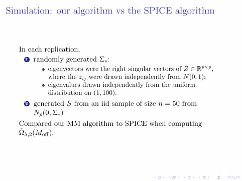
Simulation: our algorithm vs the SPICE algorithm

In each replication,1 randomly generated Σ∗:

eigenvectors were the right singular vectors of Z ∈ Rp×p,where the zij were drawn independently from N(0, 1);eigenvalues drawn independently from the uniformdistribution on (1, 100).

2 generated S from an iid sample of size n = 50 fromNp(0,Σ∗)

Compared our MM algorithm to SPICE when computingΩλ,2(Moff).

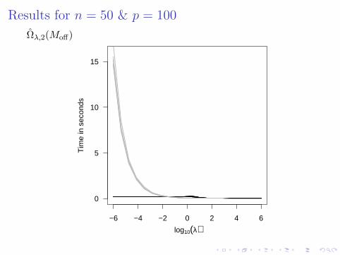
Results for n = 50 & p = 100

Ωλ,2(Moff)

−6 −4 −2 0 2 4 6

0

5

10

15

log10(λ)

Tim

e in

sec

onds

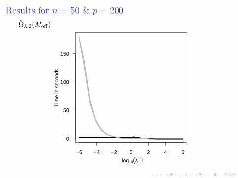
Results for n = 50 & p = 200

Ωλ,2(Moff)

−6 −4 −2 0 2 4 6

0

50

100

150

log10(λ)

Tim

e in

sec

onds

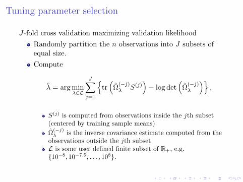
Tuning parameter selection

J-fold cross validation maximizing validation likelihood

Randomly partition the n observations into J subsets ofequal size.

Compute

λ = arg minλ∈L

J∑j=1

tr(

Ω(−j)λ S(j)

)− log det

(Ω

(−j)λ

),

S(j) is computed from observations inside the jth subset(centered by training sample means)

Ω(−j)λ is the inverse covariance estimate computed from the

observations outside the jth subsetL is some user defined finite subset of R+, e.g.10−8, 10−7.5, . . . , 108.

Classification example

Task: discriminate between metal and rocks using sonar data.

The data were taken from the UCI machine learning datarepository.

Sonar was used to produce energy measurements at p = 60frequency bands for rock and metal cylinder examples.

There were 111 metal cases and 97 rock cases.

Quadratic discriminant analysis, with regularizedcovariance estimators was applied.

Performed leave-one-out cross validation to compareclassification performance.

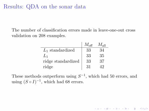
Results: QDA on the sonar data

The number of classification errors made in leave-one-out crossvalidation on 208 examples.

Moff Mall

L1 standardized 33 34L1 33 35ridge standardized 33 37ridge 31 42

These methods outperform using S−1, which had 50 errors, andusing (S I)−1, which had 68 errors.

Thank you

This talk is based on:

Rothman, A. J. and Forzani, L. (2014) Properties ofoptimizations used in penalized Gaussian likelihood inversecovariance matrix estimation. Submitted

An R package will be available soon