
Production of N Vegard-Kaplan and other triplet …Production of N 2 Vegard-Kaplan and other triplet...
25
Production of N 2 Vegard-Kaplan and other triplet band emissions in the dayglow of Titan Anil Bhardwaj * , Sonal Kumar Jain Space Physics Laboratory, Vikram Sarabhai Space Centre, Trivandrum 695022, India Abstract Recently the Cassini Ultraviolet Imaging Spectrograph (UVIS) has revealed the presence of N 2 Vegard-Kaplan (VK) band (A 3 Σ + u - X 1 Σ + g ) emissions in Titan’s dayglow limb observation. We present model calculations for the production of various N 2 triplet states (viz., A 3 Σ + u , B 3 Π g , C 3 Π u , E 3 Σ u , W 3 Δ u , and B 03 Σ u ) in the upper atmosphere of Titan. The Analytical Yield Spectra technique is used to calculate steady state photoelectron fluxes in Titan’s atmosphere, which are in agreement with those observed by the Cassini’s CAPS instrument. Considering direct electron impact excitation, inter-state cascading, and quenching effects, the population of different levels of N 2 triplet states are calculated under statistical equilibrium. Densities of all vibrational levels of each triplet state and volume production rates for various triplet states are calculated in the model. Vertically integrated overhead intensities for the same date and lighting conditions as the reported by UVIS observations for N 2 Vegard-Kaplan (A 3 Σ + u - X 1 Σ + g ), First Positive ( B 3 Π g - A 3 Σ + u ), Second Positive (C 3 Π u - B 3 Π g ), Wu-Benesch (W 3 Δ u - B 3 Π g ), and Reverse First Positive bands of N 2 are found to be 132, 114, 19, 22, and 22 R, respectively. Overhead intensities are calculated for each vibrational transition of all the triplet band emissions of N 2 , which span a wider spectrum of wavelengths from ultraviolet to infrared. The calculated limb intensities of total and prominent transitions of VK band are presented. The model limb intensity of VK emission within the 150–190 nm wavelength region is in good agreement with the Cassini UVIS observed limb profile. An assessment of the impact of solar EUV flux on the N 2 triplet band emission intensity has been made by using three different solar flux models, viz., Solar EUV Experiment (SEE), SOLAR2000 (S2K) model of Tobiska (2004), and HEUVAC model of Richards et al. (2006). The calculated N 2 VK band intensity at the peak of limb intensity due to S2K and HEUVAC solar flux models is a factor of 1.2 and 0.9, respectively, of that obtained using SEE solar EUV flux. The effects of higher N 2 density and solar zenith angle on the emission intensity are also studied. The model predicted N 2 triplet band intensities during moderate (F10.7 = 150) and high (F10.7 = 240) solar activity conditions, using SEE solar EUV flux, are a factor of 2 and 2.8, respectively, higher than those during solar minimum (F10.7 = 68) condition. Keywords: Titan, Titan Atmosphere, Ultraviolet observations, Upper atmosphere, Aeronomy, N 2 emission, Dayglow 1. Introduction The Saturnian satellite Titan, the second biggest satellite in the solar system, is in many ways the clos- est analogue to Earth. Like Earth, Titan’s atmosphere is dominated by N 2 . Hence, it is natural to expect that Titan’s airglow will be dominated by emissions of N 2 and its dissociation product N. In addition to N 2 , Titan * Corresponding author. Fax: +91 471 2706535 Email addresses: [email protected]; [email protected] (Anil Bhardwaj), [email protected] (Sonal Kumar Jain) also contains a few percent CH 4 in its atmosphere, with a mixing ratio of about 3% near 1000 km altitude (De La Haye et al., 2007; Strobel et al., 2009). The Voyager 1 Ultraviolet Spectrometer (UVS) pro- vided the first ultraviolet (UV) airglow observation of Titan in the 53–170 nm band (Broadfoot et al., 1981). The extreme ultraviolet spectrum was dominated by emissions near 95–99 nm, which were attributed to N 2 Carroll-Yoshino (CY) c 0 1 4 Σ + u – X 1 Σ + g (0, 0) and (0, 1) Rydberg bands (Strobel and Shemansky, 1982). Far ultraviolet emissions present were LBH bands of N 2 , and N and N + lines (Broadfoot et al., 1981; Strobel and Shemansky, 1982). By employing multiple scattering Published in Icarus, doi:10.1016/j.icarus.2012.01.019 arXiv:1202.2276v1 [astro-ph.EP] 10 Feb 2012
Transcript of Production of N Vegard-Kaplan and other triplet …Production of N 2 Vegard-Kaplan and other triplet...
Production of N2 Vegard-Kaplan and other triplet band emissions in thedayglow of Titan
Anil Bhardwaj∗, Sonal Kumar JainSpace Physics Laboratory, Vikram Sarabhai Space Centre, Trivandrum 695022, India
Abstract
Recently the Cassini Ultraviolet Imaging Spectrograph (UVIS) has revealed the presence of N2 Vegard-Kaplan (VK)band (A3Σ+
u −X1Σ+g ) emissions in Titan’s dayglow limb observation. We present model calculations for the production
of various N2 triplet states (viz., A3Σ+u , B3Πg, C3Πu, E3Σu, W3∆u, and B′3Σu ) in the upper atmosphere of Titan. The
Analytical Yield Spectra technique is used to calculate steady state photoelectron fluxes in Titan’s atmosphere, whichare in agreement with those observed by the Cassini’s CAPS instrument. Considering direct electron impact excitation,inter-state cascading, and quenching effects, the population of different levels of N2 triplet states are calculated understatistical equilibrium. Densities of all vibrational levels of each triplet state and volume production rates for varioustriplet states are calculated in the model. Vertically integrated overhead intensities for the same date and lightingconditions as the reported by UVIS observations for N2 Vegard-Kaplan (A3Σ+
u − X1Σ+g ), First Positive (B3Πg − A3Σ+
u ),Second Positive (C3Πu − B3Πg), Wu-Benesch (W3∆u − B3Πg), and Reverse First Positive bands of N2 are found to be132, 114, 19, 22, and 22 R, respectively. Overhead intensities are calculated for each vibrational transition of all thetriplet band emissions of N2, which span a wider spectrum of wavelengths from ultraviolet to infrared. The calculatedlimb intensities of total and prominent transitions of VK band are presented. The model limb intensity of VK emissionwithin the 150–190 nm wavelength region is in good agreement with the Cassini UVIS observed limb profile. Anassessment of the impact of solar EUV flux on the N2 triplet band emission intensity has been made by using threedifferent solar flux models, viz., Solar EUV Experiment (SEE), SOLAR2000 (S2K) model of Tobiska (2004), andHEUVAC model of Richards et al. (2006). The calculated N2 VK band intensity at the peak of limb intensity due toS2K and HEUVAC solar flux models is a factor of 1.2 and 0.9, respectively, of that obtained using SEE solar EUVflux. The effects of higher N2 density and solar zenith angle on the emission intensity are also studied. The modelpredicted N2 triplet band intensities during moderate (F10.7 = 150) and high (F10.7 = 240) solar activity conditions,using SEE solar EUV flux, are a factor of 2 and 2.8, respectively, higher than those during solar minimum (F10.7 =
68) condition.
Keywords: Titan, Titan Atmosphere, Ultraviolet observations, Upper atmosphere, Aeronomy, N2 emission, Dayglow
1. Introduction
The Saturnian satellite Titan, the second biggestsatellite in the solar system, is in many ways the clos-est analogue to Earth. Like Earth, Titan’s atmosphereis dominated by N2. Hence, it is natural to expect thatTitan’s airglow will be dominated by emissions of N2and its dissociation product N. In addition to N2, Titan
∗Corresponding author. Fax: +91 471 2706535Email addresses: [email protected];
[email protected] (Anil Bhardwaj),[email protected] (Sonal Kumar Jain)
also contains a few percent CH4 in its atmosphere, witha mixing ratio of about 3% near 1000 km altitude (DeLa Haye et al., 2007; Strobel et al., 2009).
The Voyager 1 Ultraviolet Spectrometer (UVS) pro-vided the first ultraviolet (UV) airglow observation ofTitan in the 53–170 nm band (Broadfoot et al., 1981).The extreme ultraviolet spectrum was dominated byemissions near 95–99 nm, which were attributed to N2Carroll-Yoshino (CY) c
′14 Σ+
u – X1Σ+g (0, 0) and (0, 1)
Rydberg bands (Strobel and Shemansky, 1982). Farultraviolet emissions present were LBH bands of N2,and N and N+ lines (Broadfoot et al., 1981; Strobel andShemansky, 1982). By employing multiple scattering
Published in Icarus, doi:10.1016/j.icarus.2012.01.019
arX
iv:1
202.
2276
v1 [
astr
o-ph
.EP]
10
Feb
2012
model for CY band emissions, Stevens (2001) showedthat CY (0–0) should be weak and undetectable, whileCY (0–1) should be prominent emission at 981 nm andthe features at 950 nm are N I lines. Thus, there is noneed to invoke magnetospheric electron impact excita-tion (Stevens, 2001).
After Voyager UVS, Cassini Ultraviolet ImagingSpectrograph (UVIS) provided the next observation ofTitan’s airglow in the extreme ultraviolet (EUV, 56.1–118.2 nm) and far ultraviolet (FUV, 115.5–191.3 nm)wavelengths (Ajello et al., 2007, 2008). These disk ob-servations of Titan on 13 Dec. 2004 showed the pres-ence of N2 LBH bands, atomic multiplets of NI andN+ lines, and features at 156.1 and 165.7 nm reportedlyfrom CI (Ajello et al., 2008). Recently, limb observationof Titan by UVIS obtained on 22 June 2009 has revealedthe presence of N2 Vegard-Kaplan (VK) (A3Σ+
u − X1Σ+g )
bands in the FUV spectrum (Stevens et al., 2011). Also,no CI emissions are reported to be observed. Stevenset al. (2011) showed that model emissions in the 150–190 nm VK band are consistent with UVIS observa-tions.
The N2 VK bands are a common feature in N2 at-mospheres and have been studied extensively on Earth(e.g., Cartwright, 1978; Meier, 1991; Broadfoot et al.,1997). The N2 VK bands have been observed recentlyon Mars by SPICAM aboard Mars Express (Leblancet al., 2006, 2007; Jain and Bhardwaj, 2011). Theseemission can also be observed on Venus by SPICAV on-board Venus Express (Bhardwaj and Jain, 2011), but thebright sunlit limb causes a problem in resolving the day-glow emission from scattered light from clouds.
This paper presents a detailed model calculation forthe production of N2 triplet band emissions on Titan,including the recently observed N2 VK bands. Themodel includes interstate cascading and quenching, anduses the Analytical Yield Spectra approach for the cal-culation of electron impact excitation of triplet bands,and is similar to the model used for studying the N2triplet emissions on Mars (Jain and Bhardwaj, 2011)and Venus (Bhardwaj and Jain, 2011). We also presentthe overhead emission intensities of triplet bands, whichlie in ultraviolet, visible, and infrared wavelengths. Thecalculated limb profile of N2 VK 150–190 nm emissionis compared with the Cassini UVIS observation. Impacton the intensity of N2 triplet emissions due to changesin the solar EUV flux model, solar activity, and Titan’sN2 density are discussed.
The N2 triplet band emissions span a wide spectrumof electromagnetic radiation covering EUV-FUV-MUV,visible, and infrared (Jain and Bhardwaj, 2011; Bhard-waj and Jain, 2011). Major emissions in N2 VK band lie
in the wavelength range 200-400 nm, and a few signif-icant emissions in the visible. N2 triplet First Positive(B → A), Wu-Benesch (W → B), and B′ → B bandshave prominent emissions in the infrared region. Thus,beside observations of Titan’s dayglow by the CassiniUVIS in EUV and FUV region, the Cassini Visual andInfrared Mapping Spectrometer (VIMS), which has awide spectral range 300–5100 nm (Brown et al., 2004)and Imagining Science Subsystem (ISS, 250–1100 nm)(Porco et al., 2004), might be able to detect some of thebright emissions of N2 triplet bands in the MUV, visible,and infrared wavelengths predicted by our model. Themodel calculations presented in the paper would also beuseful for any N2-containing planetary atmospheres.
2. Model Input
The N2 density profile in our model is basedon the observation made by Huygens AtmosphericStructure Instrument (HASI) on-board Huygens probe(Fulchignoni et al., 2005). Following the approach ofStevens et al. (2011), the density of N2 is reduced by afactor of 3.1 to bring the HASI N2 density at 950 km tothe level of measured density by Ion and Neutral MassSpectrometer (INMS) (De La Haye et al., 2007) aboardthe Cassini spacecraft. Since reduction in N2 density af-fects the altitude of peak production of N2 triplet bands,the effect of higher N2 density on emission intensitiesis discussed in the Section 4.3. Density of CH4 in ourmodel is based on the UVIS stellar occultation experi-ment reported by Shemansky et al. (2005).
Photoabsorption and photoionization cross sectionsof N2 and CH4 are taken from photo-cross sectionsand rate coefficients database (http://amop.space.swri.edu) (Huebner et al., 1992). The branching ra-tios for excited states of N+
2 and CH+4 are taken from
Avakyan et al. (1998). Franck-Condon factors and tran-sition probabilities required for calculating the intensityof a specific band ν′ − ν′′ of N2 are taken from Gilmoreet al. (1992). Inelastic cross sections for the electronimpact on N2 are taken from Jackman et al. (1977), ex-cept for the triplet states, which are taken from Itikawa(2006), and fitted analytically for ease of usage in themodel (Jackman et al., 1977; Bhardwaj and Jain, 2009,2011; Jain and Bhardwaj, 2011). The fitted parametersare given in Jain and Bhardwaj (2011).
The solar EUV flux is a crucial input required in mod-elling the upper atmospheric dayglow emissions. Thesolar EUV flux directly controls the photoelectron pro-duction rate, and hence the intensity of emission in theplanetary atmosphere that is produced by electron im-pact excitation, like N2 triplet band emissions, since
2
all transitions between the triplet states of N2 and theground state are spin forbidden. We have used the solarirradiance measured at Earth (between 2.5 to 120.5 nm)by Solar EUV Experiment (SEE, Version 10.2) (Woodset al., 2005; Lean et al., 2011) on 23 June 2009 (F10.7= 68) at 1 nm spectral resolution. The solar flux hasbeen scaled to the Sun-Titan distance (9.57 AU) to ac-count for the weaker flux on Titan. To evaluate the im-pact of solar EUV flux model on emission intensitieswe have also used solar EUV flux from SOLAR2000(S2K) v.2.36 model of Tobiska (2004) and HEUVACsolar EUV flux model of Richards et al. (2006) for thesame day. All calculations are made at solar zenith an-gle of 60◦ unless otherwise mentioned in the text.
107
108
109
1010
0 10 20 30 40 50 60 70 80 90 0
1
2
3
4
5
6
Sola
r E
UV
Flu
x (
photo
ns
cm
−2 s
−1)
Rati
o o
f S
2K
to S
EE
Sola
r F
lux
SEE S2K S2K/SEE
107
108
109
1010
0 10 20 30 40 50 60 70 80 90 0
1
2
3
4
5
6
Sola
r E
UV
Flu
x (
photo
ns
cm
−2 s
−1)
Rati
o o
f H
EU
VA
C t
o S
EE
Sola
r F
lux
Wavelength (nm)
SEEHEUVAC
HEUVAC/SEE
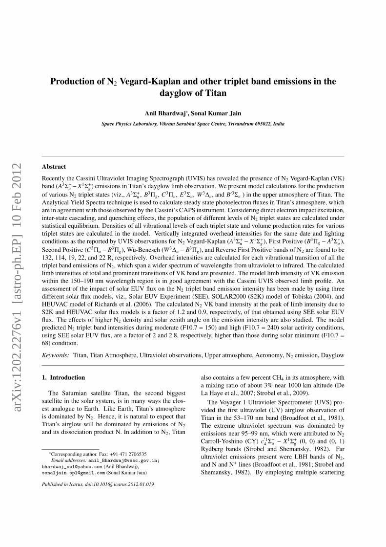
Figure 1: Comparison of SEE, S2K, and HEUVAC solar EUV fluxmodels on 23 June 2009 at 1 AU. (top) SEE solar EUV flux comparedwith S2K. (bottom) SEE solar EUV flux comparison with HEUVAC.The ratio of solar EUV fluxes is also shown with magnitude on rightside Y-axis. Thin solid horizontal line depicts the S2K/SEE andHEUVAC/SEE solar flux ratio = 1.
Figure 1 (top panel) shows the solar EUV fluxes at1 AU generated using SEE and S2K model on 23 June
2009. Ratio of S2K and SEE solar EUV flux is alsoshown in the figure. Above 60 nm the SEE and S2Kmodel solar EUV fluxes are in general agreement witheach other, but below 60 nm the solar flux of S2K modelis higher than that from SEE model. Higher EUV fluxat shorter wavelengths would result in larger number ofhigher energy photoelectrons; hence, volume produc-tion rates calculated using S2K solar EUV flux is ex-pected to be higher than that obtained using SEE solarEUV flux (see Section 4.1).
Figure 1 (bottom panel) shows the comparison ofSEE solar EUV flux with the solar flux calculated us-ing HEUVAC model, with both the daily F10.7 andthe F10.7–81 days average values set to 68 (in units of10−22 W m−2 Hz−1), conditions appropriate for the dateof the UVIS limb observations reported by Stevens et al.(2011). Since the HEUVAC model provides solar fluxup to 105 nm only, the flux in the 105–120.5 nm rangeis assumed the same as that in the SEE model. Since thesolar flux at higher (> 105 nm) wavelengths does notcontribute to the photoelectron production, the inclu-sion of SEE solar flux in the HEUVAC model at wave-lengths higher than 105 nm would not affect our calcu-lation results. At wavelength above 30 nm HEUVACsolar fluxes are smaller than those of SEE model, butat shorter (< 30 nm) wavelengths HEUVAC fluxes arehigher than SEE model fluxes. At a few shorter (< 15nm) wavelengths HEUVAC solar fluxes are as high as afactor of 4 compared to SEE solar flux. The photoelec-trons produced due to larger solar fluxes at shorter wave-lengths in HEUVAC model would result in larger num-ber of higher energy photoelectrons that can go deeperin the atmosphere, hence a significant lowering of thepeak of volume production rate is expected when theHEUVAC solar EUV flux is used (see following sec-tion).
3. Results and discussion
3.1. Photoelectron Flux
To calculate the photoelectron flux we have adoptedthe Analytical Yield Spectra (AYS) technique (cf. Sing-hal and Haider, 1984; Bhardwaj and Singhal, 1990;Bhardwaj et al., 1990, 1996; Singhal and Bhardwaj,1991; Bhardwaj, 1999, 2003; Bhardwaj and Michael,1999a,b). The AYS is the analytical representation ofnumerical yield spectra obtained using the Monte Carlomodel (cf. Singhal et al., 1980; Singhal and Bhardwaj,1991; Bhardwaj and Michael, 1999a,b; Bhardwaj andJain, 2009). Using AYS the photoelectron flux has been
3
10-5
10-4
10-3
10-2
10-1
100
0 10 20 30 40 50 60 70 80 90 100
Photo
elec
tron P
roduct
ion R
ate
(cm
-3 e
V-1
s-1)
Energy (eV)
23 June 2009
SZA = 60o
1100 km900 km
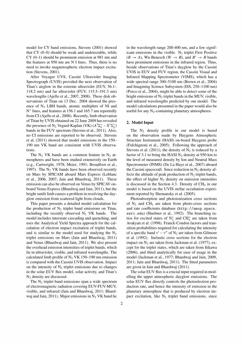
Figure 2: Calculated photoelectron production spectrum at 1100 and900 km at SZA = 60◦ using SEE solar EUV flux on 23 June 2009.
calculated as (e.g., Singhal and Haider, 1984; Bhardwajand Michael, 1999b)
φ(Z, E) =
∫ 100
Wkl
Q(Z, E)U(E, E0)∑l
nl(Z)σlT (E)dE0 (1)
where σlT (E) is the total inelastic cross section for thelth gas, at energy E, nl(Z) is its density at altitude Z,Wkl is the threshold of kth excited state of gas l, andU(E, E0) is the two-dimensional AYS, which embodiesthe non-spatial information of electron degradation pro-cess. It represents the equilibrium number of electronsper unit energy at an energy E resulting from the localenergy degradation of an incident electron of energy E0.For the N2 gas it is given as (Singhal et al., 1980)
U(E, E0) = C0 + C1(Ek + K)/[(E − M)2 + L2]. (2)
Here C0, C1, K, M, and L are the fitted parameterswhich are independent of the energy, and whose valuesare given by Singhal et al. (1980). The term Q(Z, E)in equation (1) is the primary photoelectron produc-tion rate (cf. Bhardwaj and Singhal, 1990; Michael andBhardwaj, 1997; Bhardwaj, 2003; Jain and Bhardwaj,2011). Figure 2 shows the calculated energy spectrumfor photoelectron production at 900 and 1100 km on23 June 2009 at SZA=60◦ using SEE solar EUV flux.Prominent peaks around 24–26 eV are due to the ioniza-tion of N2 in different excited states by the solar He IILyman-α line at 303.78 Å. Photoelectron energy spec-trum below 25 eV at altitude of 900 km is smaller thanthat at 1100 km, since electrons below 25 eV mainlyproduced by solar EUV photons > 30 nm which are at-tenuated at higher altitudes (> 900 km). Higher energy
photons can still penetrate deeper in the atmosphereand attain unit optical depth at lower altitudes (< 1100km). That is why photoelectron production spectrum athigher energies (> 50 eV) is higher at 900 km comparedto electron spectrum at 1100 km.
During the degradation of photoelectrons in the atmo-sphere of Titan we have not considered CH4 since N2 isthe dominant species. Contribution of CH4, which ishaving a mixing ratio of ∼3% near 1000 km, to the pho-toelectron flux is less than 10% (Stevens et al., 2011).The effect of omitting the CH4 contribution in the pho-toelectron production rate is less than 5% in our calcu-lation. Stevens et al. (2011) also have stated that ne-glecting the CH4 contribution in the calculation of pho-toelectron production rate results in only less than 5%enhancement in the EUV and FUV volume productionrates for the UVIS observation conditions.
102
103
104
105
106
107
108
109
10 20 30 40 50 60 70 80 90 100
Ph
oto
elec
tro
n F
lux
(cm
-2 e
V-1
s-1)
23 June 2009
SZA = 60o
1100 km
SEES2K
HEUVAC
101
102
103
104
105
106
107
108
109
10 20 30 40 50 60 70 80 90 100
Photo
elec
tron F
lux (
cm-2
eV
-1s-1
)
Energy (eV)
23 June 2009
SZA = 60o
1100 km
900 km
800 km
SEEStevens-model
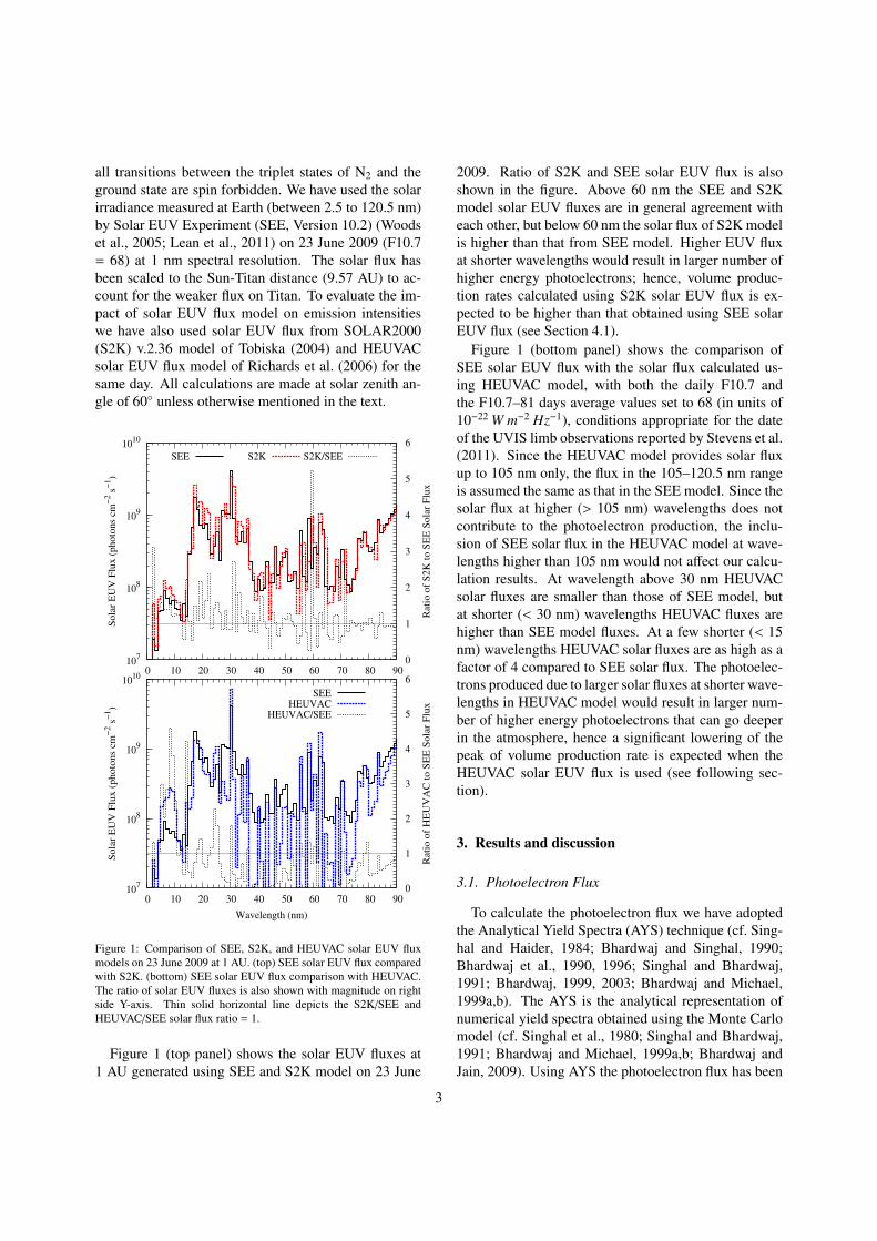
Figure 3: (top panel) Model calculated photoelectron flux at 1100km using SEE, SOLAR2000 (S2K), and HEUVAC solar flux models.(bottom panel) Comparison of model calculated photoelectron fluxesusing SEE solar EUV flux at 800, 900, and 1100 km with those ofStevens et al. (2011).
4
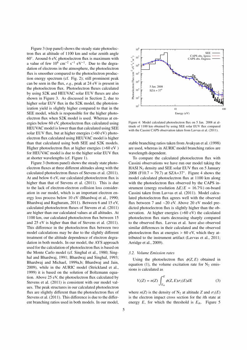
Figure 3 (top panel) shows the steady state photoelec-tron flux at altitude of 1100 km and solar zenith angle60◦. Around 6 eV, photoelectron flux is maximum witha value of few 108 cm−2 s−1 eV−1. Due to the degra-dation of electrons in the atmosphere, the photoelectronflux is smoother compared to the photoelectron produc-tion energy spectrum (cf. Fig. 2); still prominent peakcan be seen in the flux, e.g., peak at 24 eV is present inthe photoelectron flux. Photoelectron fluxes calculatedby using S2K and HEUVAC solar EUV fluxes are alsoshown in Figure 3. As discussed in Section 2, due tohigher solar EUV flux in the S2K model, the photoion-ization yield is slightly higher compared to that in theSEE model, which is responsible for the higher photo-electron flux when S2K model is used. Whereas at en-ergies below 60 eV, photoelectron flux calculated usingHEUVAC model is lower than that calculated using SEEsolar EUV flux, but at higher energies (>60 eV) photo-electron flux calculated using HEUVAC model is higherthan that calculated using both SEE and S2K models.Higher photoelectron flux at higher energies (>60 eV )for HEUVAC model is due to the higher solar EUV fluxat shorter wavelengths (cf. Figure 1).
Figure 3 (bottom panel) shows the steady state photo-electron fluxes at three different altitudes along with thecalculated photoelectron fluxes of Stevens et al. (2011).At and below 6 eV, our calculated photoelectron flux ishigher than that of Stevens et al. (2011). This is dueto the lack of electron-electron collision loss consider-ation in our model, which is an important electron en-ergy loss process below 10 eV (Bhardwaj et al., 1990;Bhardwaj and Raghuram, 2011). Between 6 and 15 eV,calculated photoelectron fluxes of Stevens et al. (2011)are higher than our calculated values at all altitudes. At1100 km, our calculated photoelectron flux between 15and 25 eV is higher than that of Stevens et al. (2011).This difference in the photoelectron flux between twomodel calculations may be due to the slightly differenttreatment of the altitude dependence of electron degra-dation in both models. In our model, the AYS approachused for the calculation of photoelectron flux is based onthe Monte Carlo model (cf. Singhal et al., 1980; Sing-hal and Bhardwaj, 1991; Bhardwaj and Singhal, 1993;Bhardwaj and Michael, 1999a,b; Bhardwaj and Jain,2009), while in the AURIC model (Strickland et al.,1999) it is based on the solution of Boltzmann equa-tion. Above 25 eV, the photoelectron flux calculated byStevens et al. (2011) is consistent with our model val-ues. The peak structures in our calculated photoelectronflux are slightly different than the photoelectron flux ofStevens et al. (2011). This difference is due to the differ-ent branching ratios used in both models. In our model,
101
102
103
104
105
106
107
108
10 100
Photo
elec
tron F
lux (
cm-2
eV
-1s-1
sr-1
)
Energy (eV)
5 Jan. 2008
SZA = 37o
SEECAPS obs. Igress
CAPS obs. Engress
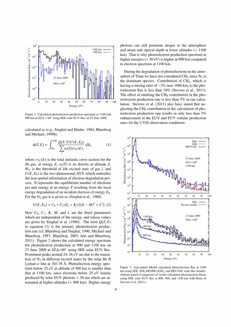
Figure 4: Model calculated photoelectron flux on 5 Jan. 2008 at al-titude of 1100 km obtained by using SEE solar EUV flux comparedwith the Cassini CAPS observation taken from Lavvas et al. (2011).
stable branching ratios taken from Avakyan et al. (1998)are used, whereas in AURIC model branching ratios arewavelength dependent.
To compare the calculated photoelectron flux withCassini observations we have run our model taking theHASI N2 density and SEE solar EUV flux on 5 January2008 (F10.7 = 79.7) at SZA=37◦. Figure 4 shows themodel calculated photoelectron flux at 1100 km alongwith the photoelectron flux observed by the CAPS in-strument (energy resolution ∆E/E = 16.7%) on-boardCassini taken from Lavvas et al. (2011). Model calcu-lated photoelectron flux agrees well with the observedflux between 7 and ∼20 eV. Above 20 eV model pre-dicted photoelectron flux is slightly higher than the ob-servation. At higher energies (>60 eV) the calculatedphotoelectron flux starts decreasing sharply comparedto the observed flux. Lavvas et al. have also observedsimilar differences in their calculated and the observedphotoelectron flux at energies > 60 eV, which they at-tributed to the instrument artifact (Lavvas et al., 2011;Arridge et al., 2009).
3.2. Volume Emission rates
Using the photoelectron flux φ(Z, E) obtained inequation (1), the volume excitation rate for N2 emis-sions is calculated as
Vi(Z) = n(Z)∫ E
Eth
φ(Z, E)σi(E)dE (3)
where n(Z) is the density of N2 at altitude Z and σi(E)is the electron impact cross section for the ith state atenergy E, for which the threshold is Eth. Figure 5
5
600
700
800
900
1000
1100
1200
1300
1400
1500
1600
10-3
10-2
10-1
100
101
Alt
itude (
km
)
Volume Production Rate (cm-3
s-1
)
E3Σu
B′3Σu
W3∆u
C3Πu
A3Σu+
B3Πg
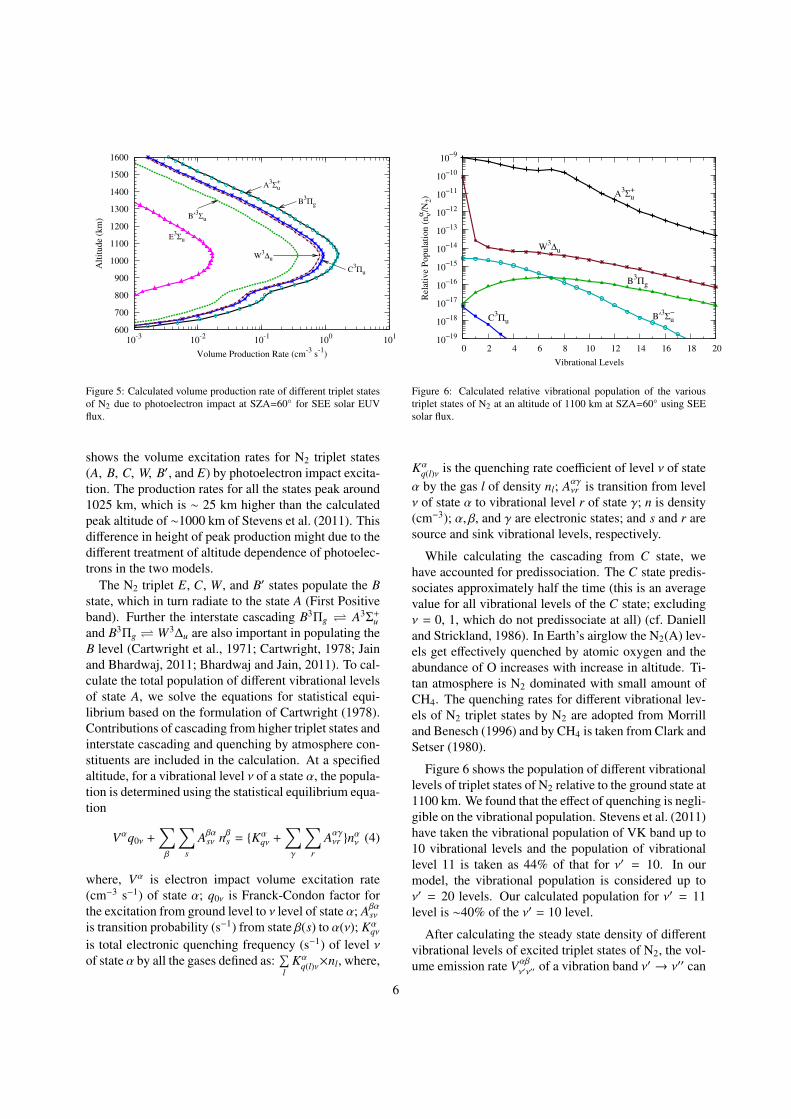
Figure 5: Calculated volume production rate of different triplet statesof N2 due to photoelectron impact at SZA=60◦ for SEE solar EUVflux.
shows the volume excitation rates for N2 triplet states(A, B, C, W, B′, and E) by photoelectron impact excita-tion. The production rates for all the states peak around1025 km, which is ∼ 25 km higher than the calculatedpeak altitude of ∼1000 km of Stevens et al. (2011). Thisdifference in height of peak production might due to thedifferent treatment of altitude dependence of photoelec-trons in the two models.
The N2 triplet E, C, W, and B′ states populate the Bstate, which in turn radiate to the state A (First Positiveband). Further the interstate cascading B3Πg A3Σ+
uand B3Πg W3∆u are also important in populating theB level (Cartwright et al., 1971; Cartwright, 1978; Jainand Bhardwaj, 2011; Bhardwaj and Jain, 2011). To cal-culate the total population of different vibrational levelsof state A, we solve the equations for statistical equi-librium based on the formulation of Cartwright (1978).Contributions of cascading from higher triplet states andinterstate cascading and quenching by atmosphere con-stituents are included in the calculation. At a specifiedaltitude, for a vibrational level ν of a state α, the popula-tion is determined using the statistical equilibrium equa-tion
Vαq0ν +∑β
∑s
Aβαsν nβs = {Kα
qν +∑γ
∑r
Aαγνr }nαν (4)
where, Vα is electron impact volume excitation rate(cm−3 s−1) of state α; q0ν is Franck-Condon factor forthe excitation from ground level to ν level of state α; Aβα
sνis transition probability (s−1) from state β(s) to α(ν); Kα
qν
is total electronic quenching frequency (s−1) of level νof state α by all the gases defined as:
∑l
Kαq(l)ν×nl, where,
10−19
10−18
10−17
10−16
10−15
10−14
10−13
10−12
10−11
10−10
10−9
0 2 4 6 8 10 12 14 16 18 20
Rel
ativ
e P
opula
tion (
nνα
/N2)
Vibrational Levels
A3Σu
+
W3∆u
B3Πg
B′3Σu
−C
3Πu
Figure 6: Calculated relative vibrational population of the varioustriplet states of N2 at an altitude of 1100 km at SZA=60◦ using SEEsolar flux.
Kαq(l)ν is the quenching rate coefficient of level ν of state
α by the gas l of density nl; Aαγνr is transition from level
ν of state α to vibrational level r of state γ; n is density(cm−3); α, β, and γ are electronic states; and s and r aresource and sink vibrational levels, respectively.
While calculating the cascading from C state, wehave accounted for predissociation. The C state predis-sociates approximately half the time (this is an averagevalue for all vibrational levels of the C state; excludingν = 0, 1, which do not predissociate at all) (cf. Danielland Strickland, 1986). In Earth’s airglow the N2(A) lev-els get effectively quenched by atomic oxygen and theabundance of O increases with increase in altitude. Ti-tan atmosphere is N2 dominated with small amount ofCH4. The quenching rates for different vibrational lev-els of N2 triplet states by N2 are adopted from Morrilland Benesch (1996) and by CH4 is taken from Clark andSetser (1980).
Figure 6 shows the population of different vibrationallevels of triplet states of N2 relative to the ground state at1100 km. We found that the effect of quenching is negli-gible on the vibrational population. Stevens et al. (2011)have taken the vibrational population of VK band up to10 vibrational levels and the population of vibrationallevel 11 is taken as 44% of that for ν′ = 10. In ourmodel, the vibrational population is considered up toν′ = 20 levels. Our calculated population for ν′ = 11level is ∼40% of the ν′ = 10 level.
After calculating the steady state density of differentvibrational levels of excited triplet states of N2, the vol-ume emission rate Vαβ
ν′ν′′ of a vibration band ν′ → ν′′ can
6
600
700
800
900
1000
1100
1200
1300
1400
1500
1600
10-2
10-1
100
101
102
Alt
itude (
km
)
Volume Emission Rate (cm-3
s-1
)
Solar Maximum (SEE)
S2K
SEE
HEUVAC
130-150 nm (× 50)
150-190 nm
400-800 nm
200-300 nm
300-400 nm
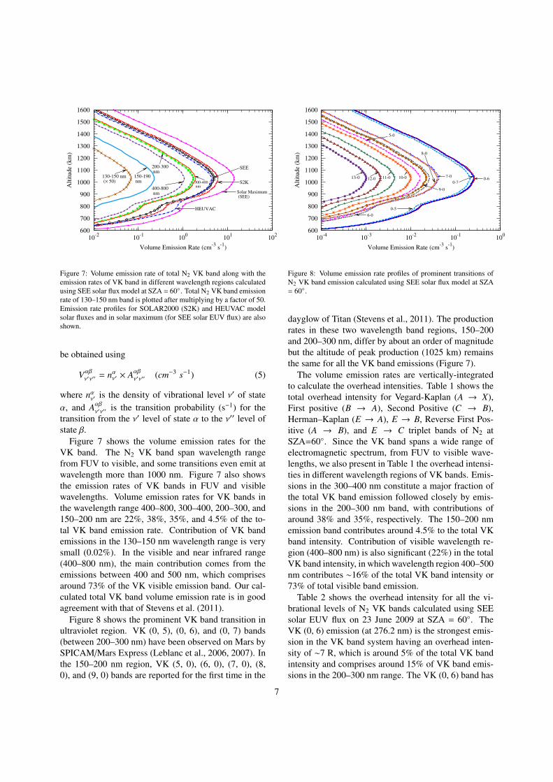
Figure 7: Volume emission rate of total N2 VK band along with theemission rates of VK band in different wavelength regions calculatedusing SEE solar flux model at SZA = 60◦. Total N2 VK band emissionrate of 130–150 nm band is plotted after multiplying by a factor of 50.Emission rate profiles for SOLAR2000 (S2K) and HEUVAC modelsolar fluxes and in solar maximum (for SEE solar EUV flux) are alsoshown.
be obtained using
Vαβν′ν′′ = nαν′ × Aαβ
ν′ν′′ (cm−3 s−1) (5)
where nαν′ is the density of vibrational level ν′ of stateα, and Aαβ
ν′ν′′ is the transition probability (s−1) for thetransition from the ν′ level of state α to the ν′′ level ofstate β.
Figure 7 shows the volume emission rates for theVK band. The N2 VK band span wavelength rangefrom FUV to visible, and some transitions even emit atwavelength more than 1000 nm. Figure 7 also showsthe emission rates of VK bands in FUV and visiblewavelengths. Volume emission rates for VK bands inthe wavelength range 400–800, 300–400, 200–300, and150–200 nm are 22%, 38%, 35%, and 4.5% of the to-tal VK band emission rate. Contribution of VK bandemissions in the 130–150 nm wavelength range is verysmall (0.02%). In the visible and near infrared range(400–800 nm), the main contribution comes from theemissions between 400 and 500 nm, which comprisesaround 73% of the VK visible emission band. Our cal-culated total VK band volume emission rate is in goodagreement with that of Stevens et al. (2011).
Figure 8 shows the prominent VK band transition inultraviolet region. VK (0, 5), (0, 6), and (0, 7) bands(between 200–300 nm) have been observed on Mars bySPICAM/Mars Express (Leblanc et al., 2006, 2007). Inthe 150–200 nm region, VK (5, 0), (6, 0), (7, 0), (8,0), and (9, 0) bands are reported for the first time in the
600
700
800
900
1000
1100
1200
1300
1400
1500
1600
10-4
10-3
10-2
10-1
100
Alt
itude (
km
)
Volume Emission Rate (cm-3
s-1
)
13-0 12-0 11-0 10-0
5-0
9-0
6-0
8-0
7-0
0-5
0-70-6
Figure 8: Volume emission rate profiles of prominent transitions ofN2 VK band emission calculated using SEE solar flux model at SZA= 60◦.
dayglow of Titan (Stevens et al., 2011). The productionrates in these two wavelength band regions, 150–200and 200–300 nm, differ by about an order of magnitudebut the altitude of peak production (1025 km) remainsthe same for all the VK band emissions (Figure 7).
The volume emission rates are vertically-integratedto calculate the overhead intensities. Table 1 shows thetotal overhead intensity for Vegard-Kaplan (A → X),First positive (B → A), Second Positive (C → B),Herman–Kaplan (E → A), E → B, Reverse First Pos-itive (A → B), and E → C triplet bands of N2 atSZA=60◦. Since the VK band spans a wide range ofelectromagnetic spectrum, from FUV to visible wave-lengths, we also present in Table 1 the overhead intensi-ties in different wavelength regions of VK bands. Emis-sions in the 300–400 nm constitute a major fraction ofthe total VK band emission followed closely by emis-sions in the 200–300 nm band, with contributions ofaround 38% and 35%, respectively. The 150–200 nmemission band contributes around 4.5% to the total VKband intensity. Contribution of visible wavelength re-gion (400–800 nm) is also significant (22%) in the totalVK band intensity, in which wavelength region 400–500nm contributes ∼16% of the total VK band intensity or73% of total visible band emission.
Table 2 shows the overhead intensity for all the vi-brational levels of N2 VK bands calculated using SEEsolar EUV flux on 23 June 2009 at SZA = 60◦. TheVK (0, 6) emission (at 276.2 nm) is the strongest emis-sion in the VK band system having an overhead inten-sity of ∼7 R, which is around 5% of the total VK bandintensity and comprises around 15% of VK band emis-sions in the 200–300 nm range. The VK (0, 6) band has
7
been observed on Mars (Leblanc et al., 2007; Jain andBhardwaj, 2011). In the dayglow spectrum of Titan VK(7, 0) transition is the strongest emission observed byCassini UVIS. For the VK (7, 0) band the model calcu-lated overhead intensity is 1.1 R, which is 0.8% of thetotal VK band intensity.
The calculated overhead intensities of N2 First Posi-tive (1P) transitions are presented in Table 3. Prominenttransitions in this band lies above 600 nm. The 1P (1, 0)emission at 888.3 nm is the brightest followed by (0, 0)emission at 1046.9 nm, which contribute around 13%and 9%, respectively, to the total 1P emission. Emis-sions between 600 and 800 nm wavelength consist ofabout 50% of the total 1P band system. The calculatedoverhead intensities of Second Positive (2P) band tran-sitions are presented in Table 4. Major portion of 2Pband emission lies in wavelengths between 300 and 400nm, which is more than 90% of the total 2P band over-head intensity. Prominent emissions in the 2P band sys-tem are (0, 0), (0, 1), (0, 2), and (1, 0) transitions, havingoverhead intensities of around 6.5, 4.5, 1.8, and 1.7 R,thus contributing around 34, 24, 9, and 9%, respectively,to the total 2P emission.
Tables 5 and 6 show the calculated overhead intensi-ties of Wu-Benesch (W → B) and B′ → B band emis-sions, respectively. Most of the emissions in W → Bband are in infrared region with a little or negligible con-tribution from emissions below 800 nm. Similar is thecase in B′ → B band system. Table 7 shows the calcu-lated overhead intensities of Herman–Kaplan (E → A),E → B, and E → C bands of N2, and Table 8 showsthe overhead intensities of Reverse First Positive (R1P)band emissions. Prominent emissions in the R1P bandsystem are in infrared region, with (9, 0) emission be-ing the strongest having the overhead intensity of 1.9 R,which is around 9% of the total R1P emission.
Stevens et al. (2011) suggested that N2 VK (8, 0)emission near 165.4 nm and (11, 0) band near 156.3nm could have been misidentified as CI 165.7 and 156.1nm emissions by Ajello et al. (2008). Also, the VK (10,0) band could be the emission near 159.2 nm, whichis reported as mystery feature by Ajello et al. (2008).We calculated the overhead intensities of CI 165.7 and156.1 nm emissions due to electron impact dissociativeexcitation of CH4 by using the emission cross sectionsfrom Shirai et al. (2002). The model calculated over-head intensities of CI 156.1 and 165.7 nm emissions are1.6 × 10−3 and 3.7 × 10⁻³ R, respectively, which areabout 2 orders of magnitude lower than the VK (8, 0)and VK (11, 0) bands intensities (see Table 2). We alsoestimated the solar scattered intensities for CI 165.7 and156.1 nm using the density of atomic carbon from the
600
800
1000
1200
1400
1600
10-1
100
101
102
103
Alt
itude
(km
)
Intensity (R)
SZA=60o
300-400 nm
200-300
nm
400-800
nm
0-6
0-7
0-5
7-0
8-0
6-0
5-0
9-0
130-150 nm
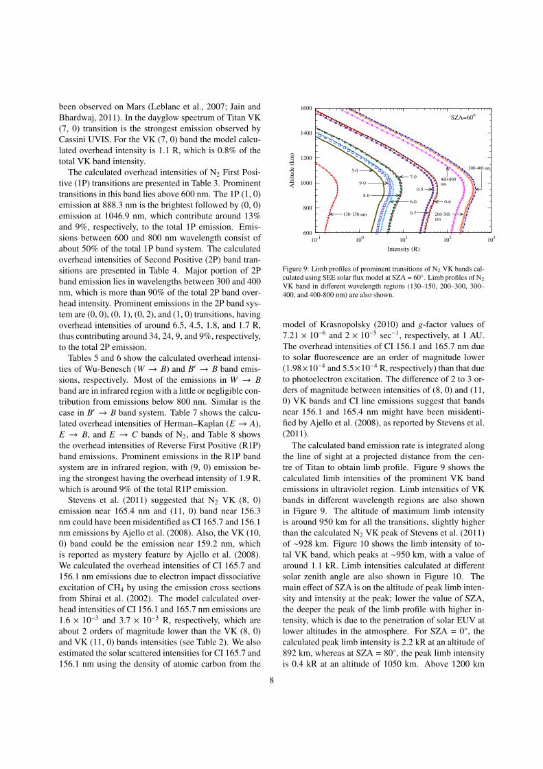
Figure 9: Limb profiles of prominent transitions of N2 VK bands cal-culated using SEE solar flux model at SZA = 60◦. Limb profiles of N2VK band in different wavelength regions (130–150, 200–300, 300–400, and 400-800 nm) are also shown.
model of Krasnopolsky (2010) and g-factor values of7.21 × 10−6 and 2 × 10⁻⁵ sec−1, respectively, at 1 AU.The overhead intensities of CI 156.1 and 165.7 nm dueto solar fluorescence are an order of magnitude lower(1.98×10⁻⁴ and 5.5×10⁻⁴ R, respectively) than that dueto photoelectron excitation. The difference of 2 to 3 or-ders of magnitude between intensities of (8, 0) and (11,0) VK bands and CI line emissions suggest that bandsnear 156.1 and 165.4 nm might have been misidenti-fied by Ajello et al. (2008), as reported by Stevens et al.(2011).
The calculated band emission rate is integrated alongthe line of sight at a projected distance from the cen-tre of Titan to obtain limb profile. Figure 9 shows thecalculated limb intensities of the prominent VK bandemissions in ultraviolet region. Limb intensities of VKbands in different wavelength regions are also shownin Figure 9. The altitude of maximum limb intensityis around 950 km for all the transitions, slightly higherthan the calculated N2 VK peak of Stevens et al. (2011)of ∼928 km. Figure 10 shows the limb intensity of to-tal VK band, which peaks at ∼950 km, with a value ofaround 1.1 kR. Limb intensities calculated at differentsolar zenith angle are also shown in Figure 10. Themain effect of SZA is on the altitude of peak limb inten-sity and intensity at the peak; lower the value of SZA,the deeper the peak of the limb profile with higher in-tensity, which is due to the penetration of solar EUV atlower altitudes in the atmosphere. For SZA = 0◦, thecalculated peak limb intensity is 2.2 kR at an altitude of892 km, whereas at SZA = 80◦, the peak limb intensityis 0.4 kR at an altitude of 1050 km. Above 1200 km
8
600
800
1000
1200
1400
1600
101
102
103
104
Alt
itude
(km
)
Intensity (R)
HASI-SEE
S2K
SZA=0
Maximum (SEE)
SZA=60
HEUVAC
SZA=80
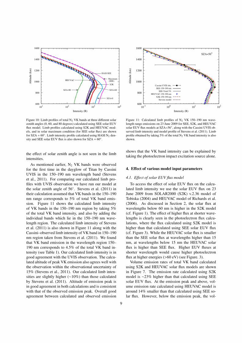
Figure 10: Limb profiles of total N2 VK bands at three different solarzenith angles (0, 60, and 80 degrees) calculated using SEE solar EUVflux model. Limb profiles calculated using S2K and HEUVAC mod-els, and in solar maximum condition (for SEE solar flux) are shownfor SZA = 60◦. Limb intensity profile calculated using HASI N2 den-sity and SEE solar EUV flux is also shown for SZA = 60◦.
the effect of solar zenith angle is not seen in the limbintensities.
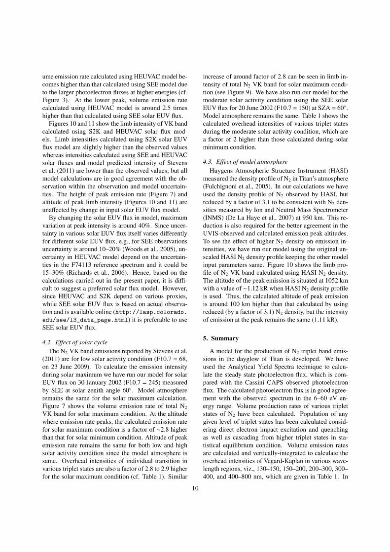
As mentioned earlier, N2 VK bands were observedfor the first time in the dayglow of Titan by CassiniUVIS in the 150–190 nm wavelength band (Stevenset al., 2011). For comparing our calculated limb pro-files with UVIS observation we have run our model atthe solar zenith angle of 56◦. Stevens et al. (2011) intheir calculation assumed that VK bands in the 150–190nm range corresponds to 5% of total VK band emis-sion. Figure 11 shows the calculated limb intensityof VK bands in the 150–190 nm region by taking 5%of the total VK band intensity, and also by adding theindividual bands which lie in the 150–190 nm wave-length region. The calculated limb intensity of Stevenset al. (2011) is also shown in Figure 11 along with theCassini–observed limb intensity of VK band in 150–190nm region taken from Stevens et al. (2011). We foundthat VK band emission in the wavelength region 150–190 nm corresponds to 4.5% of the total VK band in-tensity (see Table 1). Our calculated limb intensity is ingood agreement with the UVIS observation. The calcu-lated altitude of peak VK emission also agrees well withthe observation within the observational uncertainty of15% (Stevens et al., 2011). Our calculated limb inten-sities are slightly higher (∼10%) than those calculatedby Stevens et al. (2011). Altitude of emission peak isin good agreement in both calculations and is consistentwith that of the observed emission peak. Overall goodagreement between calculated and observed emission
600
800
1000
1200
1400
1600
10-1
100
101
102
Alt
itude
(km
)
Intensity (R)
SZA=56o
Cassini-UVIS obs.
SEE-150-190 nm
SEE-Total 5%
HEUVAC-150-190 nm
S2K-150-190 nm
Stevens model
Figure 11: Calculated limb profiles of N2 VK 150–190 nm wave-length range emissions on 23 June 2009 for SEE, S2K, and HEUVACsolar EUV flux models at SZA=56◦, along with the Cassini UVIS ob-served limb intensity and model profile of Stevens et al. (2011). Limbprofile obtained by taking 5% of the total N2 VK band intensity is alsoshown.
shows that the VK band intensity can be explained bytaking the photoelectron impact excitation source alone.
4. Effect of various model input parameters
4.1. Effect of solar EUV flux model
To access the effect of solar EUV flux on the calcu-lated limb intensity we use the solar EUV flux on 23June 2009 from SOLAR2000 (S2K) v.2.36 model ofTobiska (2004) and HEUVAC model of Richards et al.(2006). As discussed in Section 2, the solar flux atwavelengths below 60 nm is higher in the S2K model(cf. Figure 1). The effect of higher flux at shorter wave-lengths is clearly seen in the photoelectron flux calcu-lations, where the flux calculated using S2K model ishigher than that calculated using SEE solar EUV flux(cf. Figure 3). While the HEUVAC solar flux is smallerthan the SEE solar flux at wavelengths higher than 15nm, at wavelengths below 15 nm the HEUVAC solarflux is higher than SEE flux. Higher EUV fluxes atshorter wavelength would cause higher photoelectronflux at higher energies (>60 eV) (see Figure. 3).
Volume emission rates of total VK band calculatedusing S2K and HEUVAC solar flux models are shownin Figure 7. The emission rate calculated using S2Kmodel is ∼23% higher than that calculated using SEEsolar EUV flux. At the emission peak and above, vol-ume emission rate calculated using HEUVAC model isaround 14% smaller than that calculated using SEE so-lar flux. However, below the emission peak, the vol-
9
ume emission rate calculated using HEUVAC model be-comes higher than that calculated using SEE model dueto the larger photoelectron fluxes at higher energies (cf.Figure 3). At the lower peak, volume emission ratecalculated using HEUVAC model is around 2.5 timeshigher than that calculated using SEE solar EUV flux.
Figures 10 and 11 show the limb intensity of VK bandcalculated using S2K and HEUVAC solar flux mod-els. Limb intensities calculated using S2K solar EUVflux model are slightly higher than the observed valueswhereas intensities calculated using SEE and HEUVACsolar fluxes and model predicted intensity of Stevenset al. (2011) are lower than the observed values; but allmodel calculations are in good agreement with the ob-servation within the observation and model uncertain-ties. The height of peak emission rate (Figure 7) andaltitude of peak limb intensity (Figures 10 and 11) areunaffected by change in input solar EUV flux model.
By changing the solar EUV flux in model, maximumvariation at peak intensity is around 40%. Since uncer-tainty in various solar EUV flux itself varies differentlyfor different solar EUV flux, e.g., for SEE observationsuncertainty is around 10–20% (Woods et al., 2005), un-certainty in HEUVAC model depend on the uncertain-ties in the F74113 reference spectrum and it could be15–30% (Richards et al., 2006). Hence, based on thecalculations carried out in the present paper, it is diffi-cult to suggest a preferred solar flux model. However,since HEUVAC and S2K depend on various proxies,while SEE solar EUV flux is based on actual observa-tion and is available online (http://lasp.colorado.edu/see/l3_data_page.html) it is preferable to useSEE solar EUV flux.
4.2. Effect of solar cycleThe N2 VK band emissions reported by Stevens et al.
(2011) are for low solar activity condition (F10.7 = 68,on 23 June 2009). To calculate the emission intensityduring solar maximum we have run our model for solarEUV flux on 30 January 2002 (F10.7 = 245) measuredby SEE at solar zenith angle 60◦. Model atmosphereremains the same for the solar maximum calculation.Figure 7 shows the volume emission rate of total N2VK band for solar maximum condition. At the altitudewhere emission rate peaks, the calculated emission ratefor solar maximum condition is a factor of ∼2.8 higherthan that for solar minimum condition. Altitude of peakemission rate remains the same for both low and highsolar activity condition since the model atmosphere issame. Overhead intensities of individual transition invarious triplet states are also a factor of 2.8 to 2.9 higherfor the solar maximum condition (cf. Table 1). Similar
increase of around factor of 2.8 can be seen in limb in-tensity of total N2 VK band for solar maximum condi-tion (see Figure 9). We have also run our model for themoderate solar activity condition using the SEE solarEUV flux for 20 June 2002 (F10.7 = 150) at SZA = 60◦.Model atmosphere remains the same. Table 1 shows thecalculated overhead intensities of various triplet statesduring the moderate solar activity condition, which area factor of 2 higher than those calculated during solarminimum condition.
4.3. Effect of model atmosphereHuygens Atmospheric Structure Instrument (HASI)
measured the density profile of N2 in Titan’s atmosphere(Fulchignoni et al., 2005). In our calculations we haveused the density profile of N2 observed by HASI, butreduced by a factor of 3.1 to be consistent with N2 den-sities measured by Ion and Neutral Mass Spectrometer(INMS) (De La Haye et al., 2007) at 950 km. This re-duction is also required for the better agreement in theUVIS-observed and calculated emission peak altitudes.To see the effect of higher N2 density on emission in-tensities, we have run our model using the original un-scaled HASI N2 density profile keeping the other modelinput parameters same. Figure 10 shows the limb pro-file of N2 VK band calculated using HASI N2 density.The altitude of the peak emission is situated at 1052 kmwith a value of ∼1.12 kR when HASI N2 density profileis used. Thus, the calculated altitude of peak emissionis around 100 km higher than that calculated by usingreduced (by a factor of 3.1) N2 density, but the intensityof emission at the peak remains the same (1.11 kR).
5. Summary
A model for the production of N2 triplet band emis-sions in the dayglow of Titan is developed. We haveused the Analytical Yield Spectra technique to calcu-late the steady state photoelectron flux, which is com-pared with the Cassini CAPS observed photoelectronflux. The calculated photoelectron flux is in good agree-ment with the observed spectrum in the 6–60 eV en-ergy range. Volume production rates of various tripletstates of N2 have been calculated. Population of anygiven level of triplet states has been calculated consid-ering direct electron impact excitation and quenchingas well as cascading from higher triplet states in sta-tistical equilibrium condition. Volume emission ratesare calculated and vertically-integrated to calculate theoverhead intensities of Vegard-Kaplan in various wave-length regions, viz., 130–150, 150–200, 200–300, 300–400, and 400–800 nm, which are given in Table 1. In
10
addition, the vertical-integrated intensities of First Pos-itive, Second Positive, Wu-Benesch, B′ → B, E → C,E → B, E → A, and Reverse First Positive bands ofN2, are also calculated and presented in Table 1 alongwith their contributions in different wavelength regions.Vertically-integrated overhead intensities of various vi-brational transitions in triplet states are presented in Ta-bles 2 to 8.
The calculated volume emission rates are integratedalong the line of sight to calculate the limb intensity oftotal VK band. Limb profiles of various prominent tran-sitions of VK band are also calculated and presented inFigure 9. The VK band in the wavelength region 200–400 nm contribute around 73% of the total VK bandintensity, followed by the VK band in visible region(400–800 nm) which contributes around 22%. The cal-culated limb intensity profile of VK 150–190 nm bandis in good agreement with the recent Cassini UVIS-observed profile. We found that the observed intensityof VK bands can be explained by the photoelectron im-pact excitation alone (Stevens et al., 2011). The effectof change in solar zenith angle is seen in the altitude ofpeak emission as well as intensity at the emission peak.Variation in the SZA from 0◦ to 80◦ resulted in ∼18%upward shift in the altitude of emission peak, while thelimb intensity at the peak decreased by a factor of 5.5.Our calculation suggests that intensity of CI 156.1 and165.7 nm emissions due to photoelectron impact disso-ciative excitation of CH4 and fluorescence scattering ofsolar lines by carbon in Titan’s atmosphere are a feworders of magnitude smaller than the N2 VK bands 11–0 (156.3 nm) and 8–0 (165.4 nm) emission intensities,respectively.
We have also made a detailed study on the effect ofsolar EUV flux models on the N2 triplet band emissionintensities which is a step further to the calculations ofStevens et al. (2011). Emission intensities calculatedby using the S2K model are around 23% higher thanthat calculated using the SEE solar flux. The limb in-tensity at peak calculated using the HEUVAC model isaround 13% smaller than that calculated using SEE so-lar flux. The calculated intensities for moderate (F10.7= 150) and high (F10.7 = 240) solar activity conditionsare about a factor of 2 and 2.8, respectively, higher thanthose calculated during solar minimum (F10.7 = 68)condition. Calculations are also carried out taking theHASI-observed N2 density in the model atmosphere.Due to higher N2 density in the HASI observation bya factor of 3.1, the altitude of peak emission shifted up-wards by 100 km; however, the intensity at the peakremains the same.
The calculations presented in this paper will help in
understanding the production of N2 VK and other tripletband dayglow emissions on Titan as well as in other N2–containing planetary atmospheres.
AcknowledgementSonal Kumar Jain was supported by Senior Research Fel-
lowship of ISRO during the period of this work.
References
Ajello, J. M., Gustin, J., Stewart, I., Larsen, K., Esposito, L., Pryor,W., McClintock, W., Stevens, M. H., Malone, C. P., Dziczek, D.,2008. Titan airglow spectra from the Cassini Ultraviolet ImagingSpectrograph: FUV disk analysis. Geophys. Res. Lett. 35, L06102.doi:10.1029/2007GL032315.
Ajello, J. M., Stevens, M. H., Stewart, I., Larsen, K., Esposito, L., Col-well, J., McClintock, W., Holsclaw, G., Gustin, J., Pryor, W., 2007.Titan airglow spectra from Cassini Ultraviolet Imaging Spectro-graph (UVIS): EUV analysis. Geophys. Res. Lett. 34, L24204. doi:10.1029/2007GL031555.
Arridge, C. S., Gilbert, L. K., Lewis, G. R., Sittler, E. C., Jones,G. H., Kataria, D. O., Coates, A. J., Young, D. T., 2009. The effectof spacecraft radiation sources on the electron moments from theCassini CAPS electron spectrometer. Planet. Space Sci. 57, 854 –869. doi:10.1016/j.pss.2009.02.011.
Avakyan, S. V., II’in, R. N., Lavrov, V. M., Ogurtsov, G. N., 1998.In: Avakyan, S. V. (Ed.), Collision Processes and Excitation ofUV Emission from Planetary Atmospheric Gases: A Handbook ofCross Sections. Gordon and Breach science publishers.
Bhardwaj, A., 1999. On the role of solar EUV, photoelectrons, andauroral electrons in the chemistry of C(1D) and the production ofCI 1931 Å in the inner cometary coma: A case for comet P/Halley.J. Geophys. Res. 104, 1929 – 1942. doi:10.1029/1998JE900004.
Bhardwaj, A., 2003. On the solar EUV deposition in the inner co-mae of comets with large gas production rates. Geophys. Res. Lett.30 (24), 2244. doi:10.1029/2003GL018495.
Bhardwaj, A., Haider, S. A., Singhal, R. P., 1990. Auroral and pho-toelectron fluxes in cometary ionospheres. Icarus 85, 216 – 228.doi:10.1016/0019-1035(90)90112-M.
Bhardwaj, A., Haider, S. A., Singhal, R. P., 1996. Production andemissions of atomic carbon and oxygen in the inner coma of comet1P/Halley: Role of electron impact. Icarus 120, 412 – 430. doi:10.1006/icar.1996.0061.
Bhardwaj, A., Jain, S. K., 2009. Monte Carlo model of electron energydegradation in a CO2 atmosphere. J. Geophys. Res. 114, A11309.doi:10.1029/2009JA014298.
Bhardwaj, A., Jain, S. K., 2011. Calculations of N2 triplet states vibra-tional populations and band emissions in venusian dayglow. Icarus217, 752 – 758. doi:10.1016/j.icarus.2011.05.026.
Bhardwaj, A., Michael, M., 1999a. Monte Carlo model for elec-tron degradation in SO2 gas: cross sections, yield spectra andefficiencies. J. Geophys. Res. 104 (10), 24713 – 24728. doi:10.1029/1999JA900283.
Bhardwaj, A., Michael, M., 1999b. On the excitation of Io’s at-mosphere by the photoelectrons: Application of the analyticalyield spectrum of SO2. Geophys. Res. Lett. 26, 393 – 396. doi:10.1029/1998GL900320.
Bhardwaj, A., Raghuram, S., 2011. Coupled Chemistry-EmissionModel for Atomic Oxygen Green and Red-doublet Emissionsin Comet C/1996 B2 Hyakutake. Astrophys. J. In press. doi:10.1088/0004-637X/745/1/1
11
Bhardwaj, A., Singhal, R. P., 1990. Auroral and dayglow processeson Neptune. Indian Journal of Radio and Space Physics 19, 171 –176.
Bhardwaj, A., Singhal, R. P., 1993. Optically thin H Lyman al-pha production on outer planets: Low-energy proton accelera-tion in parallel electric fields and neutral H atom precipitationfrom ring current. J. Geophys. Res. 98 (A6), 9473 – 9481. doi:10.1029/92JA02400.
Broadfoot, A., Hatfield, D., Anderson, E., Stone, T., Sandel, B., Gard-ner, J., Murad, E., Knecht, D., Pike, C., Viereck, R., 1997. N2triplet band systems and atomic oxygen in the dayglow. J. Geo-phys. Res. 102 (A6), 11567 – 11584. doi:10.1029/97JA00771.
Broadfoot, A. L., Sandel, B. R., Shemansky, D. E., Holberg, J. B.,Smith, G. R., Strobel, D. F., McConnell, J. C., Kumar, S., Hunten,D. M., Atreya, S. K., Donahue, T. M., Moos, H. W., Bertaux, J. L.,Blamont, J. E., Pomphrey, R. B., Linick, S., April 1981. Extremeultraviolet observations from Voyager 1 encounter with Saturn.Science 212, 206 – 211. doi:10.1126/science.212.4491.206.
Brown, R. H. et al., 2004. The Cassini Visual and Infrared MappingSpectrometer (VIMS) Investigation. Space Science Reviews 115,111–168. doi:10.1007/s11214-004-1453-x.
Cartwright, D., Trajmar, S., Williams, W., 1971. Vibrational popula-tion of the A3Σ+
u and B3Πg states of N2 in normal auroras. J. Geo-phys. Res. 76 (34), 8368 – 8377. doi:10.1029/JA076i034p08368.
Cartwright, D. C., 1978. Vibrational populations of the excited stateof N2 under auroral condition. J. Geophys. Res. 83 (A2), 517 –321. doi:10.1029/JA083iA02p00517.
Clark, W. G., Setser, D. W., 1980. Energy transfer reactions of N2(A3Σ+
u ). 5. Quenching by hydrogen halides, methyl halides, andother molecules. J. Phys. Chm. 84 (18), 2225 – 2233.
Daniell, R., Strickland, D., 1986. Dependence of auroral mid-dle UV emissions on the incident electron spectrum and neu-tral atmosphere. J. Geophys. Res. 91 (A1), 321 – 327. doi:10.1029/JA091iA01p00321.
De La Haye, V., Waite, J. H., Johnson, R. E., Yelle, R. V., Cravens,T. E., Luhmann, J. G., Kasprzak, W. T., Gell, D. A., Magee, B.,Leblanc, F., Michael, M., Jurac, S., Robertson, I. P., Jul. 2007.Cassini Ion and Neutral Mass Spectrometer data in Titan’s upperatmosphere and exosphere: Observation of a suprathermal corona.J. Geophys. Res. 112, A07309. doi:10.1029/2006JA012222.
Fulchignoni, M. et al., 2005. In situ measurements of the physicalcharacteristics of Titan’s environment. Nature 438, 785–791. doi:10.1038/nature04314.
Gilmore, F. R., Laher, R. R., Espy, P. J., 1992. Franck-Condon fac-tors, r-centroids, electronic transition moments, and Einstein co-efficients for many nitrogen and oxygen band systems. J. Phys.Chem. Ref. Data 21, 1005 – 1107. doi:10.1063/1.555910.
Huebner, W. F., Keady, J. J., Lyon, S. P., 1992. Solar photoratesfor planetary atmospheres and atmospheric pollutants. Astrophys.Space Sci. 195 (1), 1 – 289. doi:10.1007/BF00644558.
Itikawa, Y., 2006. Cross sections for electron collisions with nitro-gen molecules. J. Phys. Chem. Ref. Data 35 (1), 31 – 53. doi:10.1063/1.1937426.
Jackman, C., Garvey, R., Green, A., 1977. Electron impact on atmo-spheric gases, I. Updated cross sections. J. Geophys. Res. 82 (32),5081 – 5090. doi:10.1029/JA082i032p05081.
Jain, S. K., Bhardwaj, A., 2011. Model calculation of N2 Vegard-Kaplan band emissions in Martian dayglow. J. Geophys. Res. 116,E07005. doi:10.1029/2010JE003778.
Krasnopolsky, V. A., 2010. The photochemical model of Titan’satmosphere and ionosphere: A version without hydrodynamicescape. Planetary and Space Science 58, 1507 – 1515. doi:10.1016/j.pss.2010.07.010.
Lavvas, P., Galand, M., Yelle, R. V., Heays, A. N., Lewis, B. R.,Lewis, G. R., Coates, A. J., 2011. Energy deposition and primary
chemical products in Titan’s upper atmosphere. Icarus 213, 233 –251. doi:10.1016/j.icarus.2011.03.001.
Lean, J. L., Woods, T. N., Eparvier, F. G., Meier, R. R., Strickland,D. J., Correira, J. T., Evans, J. S., 2011. Solar extreme ultravi-olet irradiance: Present, past, and future. J. Geophys. Res. 116,A01102. doi:10.1029/2010JA015901.
Leblanc, F., Chaufray, J. Y., Bertaux, J. L., 2007. On Martiannitrogen dayglow emission observed by SPICAM UV spectro-graph/Mars Express. Geophys. Res. Lett. 34, L02206. doi:10.1029/2006GL0284.
Leblanc, F., Chaufray, J. Y., Lilensten, J., Witasse, O., Bertaux, J.-L., 2006. Martian dayglow as seen by the SPICAM UV spec-trograph on Mars Express. J. Geophys. Res. 111, E09S11. doi:10.1029/2005JE002664.
Meier, R., 1991. Ultraviolet spectroscopy and remote sensing ofthe upper atmosphere. Space Science Reviews 58, 1–185. doi:10.1007/BF01206000.
Michael, M., Bhardwaj, A., 1997. On the dissociative ionization ofSO2 in the Io’s atmosphere. Geophys. Res. Lett. 24, 1971 – 1974.doi:10.1029/97GL02056.
Morrill, J., Benesch, W., 1996. Auroral N2 emissions and the effect ofcollisional processes on N2 triplet state vibrational populations. J.Geophys. Res. 101 (A1), 261 – 274. doi:10.1029/95JA02835.
Porco, C. C., West, R. A., Squyres, S., McEwen, A., Thomas, P., Mur-ray, C. D., Del Genio, A., Ingersoll, A. P., Johnson, T. V., Neukum,G., Veverka, J., Dones, L., Brahic, A., Burns, J. A., Haemmerle,V., Knowles, B., Dawson, D., Roatsch, T., Beurle, K., Owen, W.,2004. Cassini Imaging Science: Instrument characteristics And an-ticipated scientific investigations at Saturn. Space Sci. Rev. 115,363 – 497. doi:10.1007/s11214-004-1456-7.
Richards, P. G., Woods, T. N., Peterson, W. K., 2006. HEUVAC:A new high resolution solar EUV proxy model. Adv. Space Res.37 (2), 315 – 322. doi:10.1016/j.asr.2005.06.031.
Shemansky, D. E., Stewart, A. I. F., West, R. A., Esposito,L. W., Hallett, J. T., Liu, X., 2005. The Cassini UVIS stellarprobe of the Titan atmosphere. Science 308, 978 – 982. doi:10.1126/science.1111790.
Shirai, T., Tabata, T., Tawara, H., Itikawa, Y., 2002. Analytic crosssections for electron collisions with hydrocarbons: CH4, C2H6,C2H4, C2H2, C3H8, and C3H6. At. Data Nucl. Data Tables 80, 147– 204. doi:10.1006/adnd.2001.0878.
Singhal, R. P., Bhardwaj, A., 1991. Monte Carlo simulationof photoelectron energization in parallel electric fields: Elec-troglow on Uranus. J. Geophys. Res. 96, 15963 – 15972. doi:10.1029/90JA02749.
Singhal, R. P., Haider, S. A., 1984. Analytical Yield Spectrum ap-proach to photoelectron fluxes in the Earth’s atmosphere. J. Geo-phys. Res. 89 (A8), 6847 – 6852. doi:10.1029/JA089iA08p06847.
Singhal, R. P., Jackman, C., Green, A. E. S., 1980. Spatial aspects oflow and medium energy electron degradation in N2. J. Geophys.Res. 85 (A3), 1246 – 1254. doi:10.1029/JA085iA03p01246.
Stevens, M. H., 2001. The EUV airglow of Titan: Production and lossof N2 c′4(0) – X. J. Geophys. Res. 106, 3685 – 3689.
Stevens, M. H., Gustin, J., Ajello, J. M., Evans, J. S., Meier,R. R., Kochenash, A. J., Stephan, A. W., Stewart, A. I. F., Es-posito, L. W., McClintock, W. E., Holsclaw, G., Bradley, E. T.,Lewis, B. R., Heays, A. N., 2011. The production of Titan’s ul-traviolet nitrogen airglow. J. Geophys. Res. 116, A05304. doi:10.1029/2010JA016284.
Strickland, D. J., Bishop, J., Evans, J. S., Majeed, T., Shen, P. M.,Cox, R. J., Link, R., Huffman, R. E., 1999. Atmospheric Ultravi-olet Radiance Integrated Code (AURIC): Theory, software archi-tecture, inputs, and selected results. Journal of Quantitative Spec-troscopy & Radiative Transfer 62, 689 – 742. doi:1016/S0022-4073(98)00098-3.
12
Strobel, D. F., Atreya, S. K., Bezard, B., Ferri, F., Flasar, F. M.,Fulchignoni, M., Lellouch, E., Muller-Wodarg, I., 2009. Titan fromcassini-huygens. Springer, Ch. Atmospheric Structure and Compo-sition, pp. 235 – 257. doi:10.1007/978-1-4020-9215-2.
Strobel, D. F., Shemansky, D. E., 1982. EUV emission from Ti-tan’s upper atmosphere: Voyager 1 encounter. J. Geophys. Res.87, 1361. doi:10.1029/JA087iA03p01361.
Tobiska, W. K., 2004. SOLAR2000 irradiances for climate change,aeronomy and space system engineering. Adv. Space Res. 34, 1736– 1746. doi:10.1016/j.asr.2003.06.032.
Woods, T. N., Eparvier, F. G., Bailey, S. M., Chamberlin, P. C.,Lean, J., Rottman, G. J., Solomon, S. C., Tobiska, W. K.,Woodraska, D. L., 2005. Solar EUV Experiment (SEE): Missionoverview and first results. J. Geophys. Res. 110, A01312. doi:10.1029/2004JA010765.
13
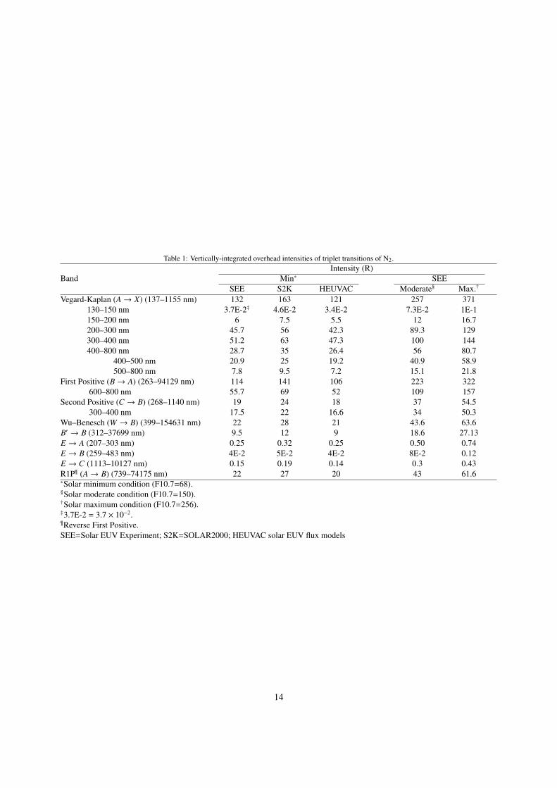
Table 1: Vertically-integrated overhead intensities of triplet transitions of N2.
BandIntensity (R)
Min∗ SEESEE S2K HEUVAC Moderate§ Max.†
Vegard-Kaplan (A→ X) (137–1155 nm) 132 163 121 257 371130–150 nm 3.7E-2‡ 4.6E-2 3.4E-2 7.3E-2 1E-1150–200 nm 6 7.5 5.5 12 16.7200–300 nm 45.7 56 42.3 89.3 129300–400 nm 51.2 63 47.3 100 144400–800 nm 28.7 35 26.4 56 80.7
400–500 nm 20.9 25 19.2 40.9 58.9500–800 nm 7.8 9.5 7.2 15.1 21.8
First Positive (B→ A) (263–94129 nm) 114 141 106 223 322600–800 nm 55.7 69 52 109 157
Second Positive (C → B) (268–1140 nm) 19 24 18 37 54.5300–400 nm 17.5 22 16.6 34 50.3
Wu–Benesch (W → B) (399–154631 nm) 22 28 21 43.6 63.6B′ → B (312–37699 nm) 9.5 12 9 18.6 27.13E → A (207–303 nm) 0.25 0.32 0.25 0.50 0.74E → B (259–483 nm) 4E-2 5E-2 4E-2 8E-2 0.12E → C (1113–10127 nm) 0.15 0.19 0.14 0.3 0.43R1P¶ (A→ B) (739–74175 nm) 22 27 20 43 61.6∗Solar minimum condition (F10.7=68).§Solar moderate condition (F10.7=150).†Solar maximum condition (F10.7=256).‡3.7E-2 = 3.7 × 10⁻².¶Reverse First Positive.SEE=Solar EUV Experiment; S2K=SOLAR2000; HEUVAC solar EUV flux models
14
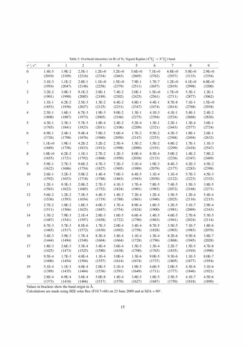
Table 2: Overhead intensities (in R) of N2 Vegard-Kaplan (A3Σ+u → X1Σ+
g ) band.
ν′ \ ν′′ 0 1 2 3 4 5 6 7 8 9
0 1.4E-5 1.9E-2 2.5E-1 1.2E+0 3.2E+0 5.6E+0 7.1E+0 6.8E+0 5.0E+0 2.9E+0(2010) (2109) (2216) (2334) (2463) (2605) (2762) (2937) (3133) (3354)
1 3.1E-3 1.1E-2 2.8E-1 1.1E+0 1.5E+0 7.9E-1 1.7E-7 1.2E+0 4.1E+0 6.0E+0(1954) (2047) (2148) (2258) (2379) (2511) (2657) (2819) (2998) (3200)
2 3.2E-2 3.0E-3 9.1E-2 2.8E-1 7.4E-2 2.0E-1 1.3E+0 1.7E+0 5.3E-1 1.2E-1(1901) (1990) (2085) (2189) (2302) (2425) (2561) (2711) (2877) (3062)
3 1.1E-1 6.2E-2 2.5E-3 1.3E-2 6.4E-2 4.8E-1 4.4E-1 8.7E-8 7.1E-1 1.5E+0(1853) (1936) (2027) (2125) (2231) (2347) (2474) (2614) (2768) (2938)
4 2.5E-1 1.6E-1 6.7E-3 1.9E-3 9.0E-2 1.3E-1 4.1E-3 4.1E-1 5.4E-1 2.4E-2(1808) (1887) (1973) (2065) (2166) (2275) (2394) (2524) (2668) (2826)
5 4.3E-1 2.3E-1 5.7E-3 1.8E-4 2.4E-2 5.2E-4 1.3E-1 2.2E-1 1.3E-4 3.6E-1(1765) (1841) (1923) (2011) (2106) (2209) (2321) (2443) (2577) (2724)
6 6.9E-1 2.4E-1 9.4E-4 7.8E-3 5.6E-4 1.7E-2 9.5E-2 4.3E-3 1.8E-1 2.6E-1(1726) (1798) (1876) (1960) (2050) (2147) (2253) (2368) (2494) (2632)
7 1.1E+0 1.9E-1 4.2E-2 3.2E-2 2.5E-4 1.5E-2 1.5E-2 4.8E-2 1.7E-1 1.1E-3(1689) (1758) (1833) (1912) (1998) (2090) (2191) (2299) (2418) (2547)
8 1.0E+0 6.2E-2 1.1E-1 2.7E-2 1.2E-3 8.0E-4 8.5E-4 5.0E-2 1.4E-2 7.8E-2(1655) (1721) (1792) (1868) (1950) (2038) (2133) (2236) (2347) (2469)
9 5.9E-1 2.7E-3 9.6E-2 4.7E-3 7.2E-3 3.1E-4 1.9E-3 8.4E-3 4.2E-3 4.5E-2(1622) (1686) (1754) (1827) (1905) (1989) (2079) (2177) (2283) (2398)
10 2.6E-1 3.2E-3 5.0E-2 1.4E-4 7.6E-3 6.4E-5 1.1E-4 1.1E-4 5.7E-3 4.5E-3(1592) (1653) (1718) (1788) (1863) (1943) (2030) (2122) (2223) (2332)
11 1.2E-1 9.3E-3 2.0E-2 2.7E-3 4.1E-3 1.7E-4 7.8E-5 7.4E-5 1.5E-3 3.8E-5(1563) (1622) (1685) (1752) (1824) (1901) (1983) (2072) (2168) (2271)
12 5.6E-2 1.2E-2 7.3E-3 4.4E-3 1.4E-3 7.2E-4 1.2E-4 1.5E-5 1.2E-4 5.4E-4(1536) (1593) (1654) (1719) (1788) (1861) (1940) (2025) (2116) (2215)
13 2.7E-2 1.0E-2 1.8E-3 4.0E-3 1.7E-4 8.9E-4 1.8E-5 1.2E-5 3.1E-7 2.9E-4(1511) (1566) (1625) (1687) (1754) (1824) (1900) (1981) (2069) (2163)
14 1.3E-2 7.9E-3 2.1E-4 2.8E-3 1.6E-5 6.6E-4 1.4E-5 4.6E-5 2.7E-6 5.3E-5(1487) (1541) (1597) (1658) (1722) (1790) (1863) (1941) (2024) (2114)
15 6.7E-3 5.7E-3 8.5E-6 1.7E-3 2.0E-4 3.4E-4 8.7E-5 3.5E-5 7.1E-7 1.8E-6(1465) (1517) (1572) (1630) (1692) (1758) (1828) (1903) (1983) (2070)
16 3.4E-3 3.9E-3 1.7E-4 8.3E-4 3.4E-4 1.1E-4 1.3E-4 8.2E-6 9.5E-6 3.8E-7(1444) (1494) (1548) (1604) (1664) (1728) (1796) (1868) (1945) (2028)
17 1.8E-3 2.6E-3 3.3E-4 3.4E-4 3.6E-4 1.5E-5 1.3E-4 2.2E-7 1.5E-5 4.7E-8(1425) (1473) (1525) (1580) (1638) (1700) (1765) (1835) (1910) (1990)
18 9.5E-4 1.7E-3 4.0E-4 1.1E-4 3.0E-4 1.3E-6 9.0E-5 9.3E-6 1.1E-5 8.0E-7(1406) (1454) (1504) (1557) (1614) (1674) (1737) (1805) (1877) (1954)
19 5.1E-4 1.1E-3 4.0E-4 2.0E-5 2.1E-4 1.9E-5 4.6E-5 2.0E-5 4.3E-6 3.1E-6(1389) (1435) (1484) (1536) (1591) (1649) (1711) (1777) (1846) (1921)
20 2.8E-4 6.9E-4 3.6E-4 5.0E-8 1.4E-4 3.8E-5 1.8E-5 2.5E-5 4.1E-7 4.5E-6(1373) (1418) (1466) (1517) (1570) (1627) (1687) (1750) (1818) (1890)
Values in brackets show the band origin in Å.Calculations are made using SEE solar flux (F10.7=68) on 23 June 2009 and at SZA = 60◦.
15
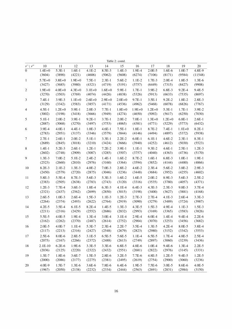
Table 2: contd.
ν′ \ ν′′ 10 11 12 13 14 15 16 17 18 19 200 1.4E+0 5.3E-1 1.6E-1 4.1E-2 8.5E-3 1.4E-3 1.9E-4 2.0E-5 1.6E-6 1.0E-7 4.8E-9
(3604) (3890) (4221) (4606) (5062) (5608) (6274) (7106) (8171) (9584) (11548)
1 5.7E+0 3.8E+0 1.9E+0 7.5E-1 2.3E-1 5.6E-2 1.1E-2 1.7E-3 2.0E-4 1.8E-5 1.3E-6(3427) (3685) (3980) (4321) (4719) (5191) (5757) (6449) (7315) (8427) (9908)
2 1.9E+0 4.0E+0 4.3E+0 3.1E+0 1.6E+0 5.9E-1 1.7E-1 3.9E-2 6.8E-3 9.2E-4 9.4E-5(3270) (3503) (3769) (4074) (4426) (4838) (5326) (5913) (6633) (7535) (8697)
3 7.4E-1 3.9E-3 1.1E+0 2.6E+0 2.9E+0 2.0E+0 9.7E-1 3.5E-1 9.2E-2 1.8E-2 2.8E-3(3129) (3342) (3583) (3857) (4171) (4536) (4962) (5468) (6078) (6826) (7767)
4 4.5E-1 1.2E+0 5.9E-1 2.0E-3 7.7E-1 1.8E+0 1.9E+0 1.2E+0 5.3E-1 1.7E-1 3.9E-2(3002) (3198) (3418) (3666) (3949) (4274) (4650) (5092) (5617) (6250) (7030)
5 5.1E-1 2.0E-2 3.9E-1 9.2E-1 3.7E-1 2.0E-2 7.0E-1 1.3E+0 1.2E+0 6.8E-1 2.6E-1(2887) (3068) (3270) (3497) (3753) (4065) (4381) (4771) (5229) (5773) (6432)
6 3.9E-4 4.0E-1 4.4E-1 1.0E-3 4.6E-1 7.5E-1 1.8E-1 8.7E-2 7.4E-1 1.1E+0 8.2E-1(2783) (2951) (3137) (3346) (3579) (3844) (4146) (4494) (4897) (5372) (5938)
7 2.7E-1 2.6E-1 2.0E-2 5.1E-1 3.3E-1 2.2E-2 6.0E-1 6.1E-1 4.6E-2 2.3E-1 8.3E-1(2689) (2845) (3018) (3210) (3424) (3666) (3940) (4252) (4612) (5030) (5523)
8 1.4E-1 5.2E-3 2.6E-1 1.2E-1 7.2E-2 3.9E-1 1.1E-1 9.3E-2 4.6E-1 2.5E-1 1.2E-3(2602) (2748) (2909) (3087) (3285) (3507) (3757) (4040) (4363) (4736) (5170)
9 1.3E-3 7.0E-2 5.1E-2 2.4E-2 1.4E-1 1.6E-2 8.7E-2 1.6E-1 6.8E-3 1.0E-1 1.9E-1(2523) (2660) (2810) (2976) (3160) (3364) (3594) (3852) (4144) (4480) (4866)
10 8.2E-3 2.1E-2 1.3E-3 4.0E-2 7.0E-3 2.8E-2 4.6E-2 2.3E-4 5.6E-2 3.8E-2 2.9E-3(2450) (2579) (2720) (2875) (3046) (3236) (3448) (3684) (3952) (4255) (4602)
11 5.8E-3 5.5E-4 8.7E-3 5.6E-3 5.3E-3 1.6E-2 1.6E-5 2.0E-2 8.9E-3 5.6E-3 2.5E-2(2383) (2505) (2638) (2783) (2743) (3120) (3316) (3535) (3780) (4057) (4371)
12 1.2E-3 7.7E-4 3.6E-3 1.8E-4 6.3E-3 4.1E-4 6.4E-3 4.3E-3 2.3E-3 9.8E-3 3.7E-4(2321) (2437) (2562) (2699) (2850) (3015) (3198) (3400) (3627) (3881) (4168)
13 2.6E-5 1.0E-3 2.6E-4 1.5E-3 1.1E-3 1.2E-3 2.7E-3 2.7E-4 4.1E-3 2.6E-4 3.3E-3(2264) (2374) (2493) (2622) (2764) (2919) (3090) (3279) (3489) (3724) (3987)
14 4.2E-5 3.5E-4 6.1E-5 8.2E-4 1.4E-5 1.3E-3 4.3E-5 1.5E-3 4.9E-4 1.1E-3 1.5E-3(2211) (2316) (2429) (2552) (2686) (2832) (2993) (3169) (3365) (3583) (3826)
15 5.5E-5 4.0E-5 1.9E-4 1.3E-4 3.0E-4 3.1E-4 2.9E-4 6.0E-4 1.4E-4 9.4E-4 2.2E-6(2162) (2262) (2370) (2487) (2614) (2752) (2904) (3070) (3253) (3456) (3682)
16 2.0E-5 4.0E-7 1.1E-4 5.3E-7 2.3E-4 2.2E-7 3.5E-4 1.3E-5 4.2E-4 8.0E-5 3.8E-4(2117) (2213) (2316) (2427) (2548) (2679) (2823) (2980) (3152) (3342) (3553)
17 2.5E-6 8.0E-6 2.8E-5 3.1E-5 6.5E-5 5.6E-5 1.1E-4 6.5E-5 1.7E-4 4.8E-5 2.5E-4(2075) (2167) (2266) (2372) (2488) (2613) (2749) (2897) (3060) (3239) (3436)
18 2.1E-10 6.2E-6 1.9E-6 3.3E-5 3.3E-6 6.8E-5 4.8E-6 1.0E-4 9.4E-6 1.3E-4 2.2E-5(2036) (2125) (2220) (2322) (2432) (2551) (2681) (2822) (2976) (3145) (3331)
19 1.3E-7 1.8E-6 3.6E-7 1.5E-5 2.8E-6 3.2E-5 7.7E-6 4.8E-5 1.2E-5 9.4E-5 1.2E-5(2000) (2086) (2177) (2275) (2381) (2495) (2619) (2754) (2900) (3060) (3236)
20 4.0E-9 1.5E-7 1.3E-6 3.6E-6 7.8E-6 6.4E-6 1.9E-5 7.5E-6 3.0E-5 8.6E-6 4.0E-5(1967) (2050) (2138) (2232) (2334) (2444) (2563) (2691) (2831) (2984) (3150)
16
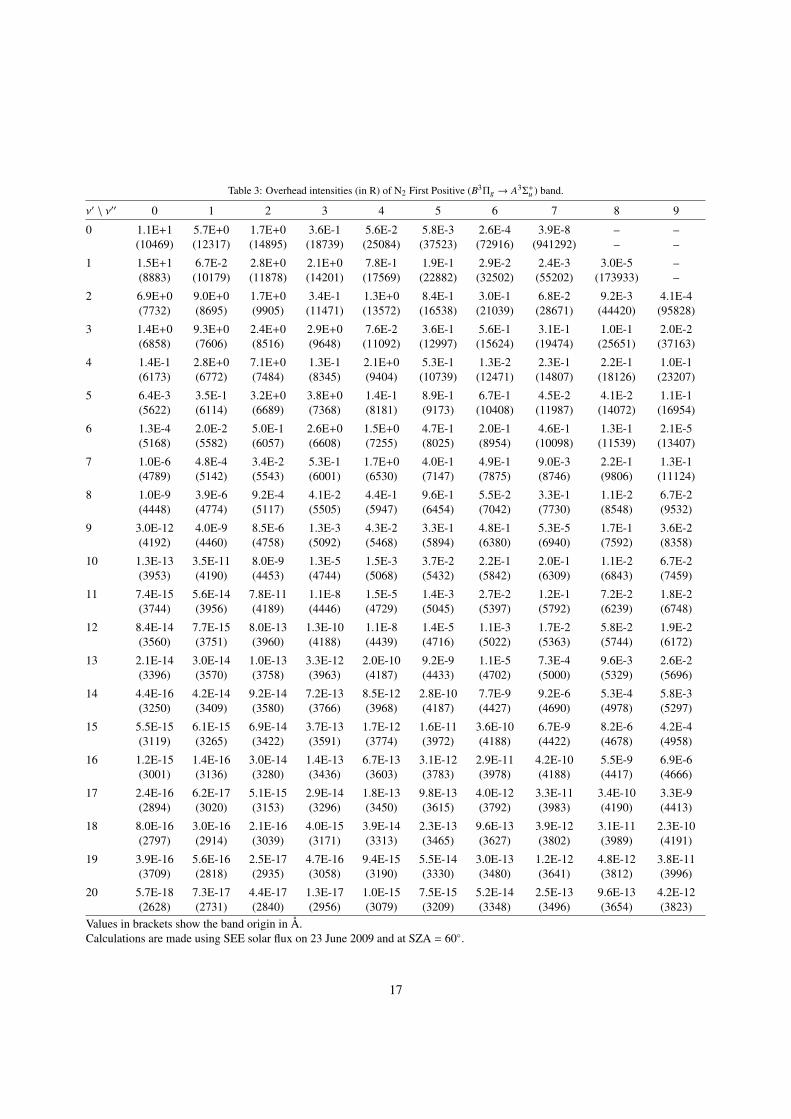
Table 3: Overhead intensities (in R) of N2 First Positive (B3Πg → A3Σ+u ) band.
ν′ \ ν′′ 0 1 2 3 4 5 6 7 8 9
0 1.1E+1 5.7E+0 1.7E+0 3.6E-1 5.6E-2 5.8E-3 2.6E-4 3.9E-8 – –(10469) (12317) (14895) (18739) (25084) (37523) (72916) (941292) – –
1 1.5E+1 6.7E-2 2.8E+0 2.1E+0 7.8E-1 1.9E-1 2.9E-2 2.4E-3 3.0E-5 –(8883) (10179) (11878) (14201) (17569) (22882) (32502) (55202) (173933) –
2 6.9E+0 9.0E+0 1.7E+0 3.4E-1 1.3E+0 8.4E-1 3.0E-1 6.8E-2 9.2E-3 4.1E-4(7732) (8695) (9905) (11471) (13572) (16538) (21039) (28671) (44420) (95828)
3 1.4E+0 9.3E+0 2.4E+0 2.9E+0 7.6E-2 3.6E-1 5.6E-1 3.1E-1 1.0E-1 2.0E-2(6858) (7606) (8516) (9648) (11092) (12997) (15624) (19474) (25651) (37163)
4 1.4E-1 2.8E+0 7.1E+0 1.3E-1 2.1E+0 5.3E-1 1.3E-2 2.3E-1 2.2E-1 1.0E-1(6173) (6772) (7484) (8345) (9404) (10739) (12471) (14807) (18126) (23207)
5 6.4E-3 3.5E-1 3.2E+0 3.8E+0 1.4E-1 8.9E-1 6.7E-1 4.5E-2 4.1E-2 1.1E-1(5622) (6114) (6689) (7368) (8181) (9173) (10408) (11987) (14072) (16954)
6 1.3E-4 2.0E-2 5.0E-1 2.6E+0 1.5E+0 4.7E-1 2.0E-1 4.6E-1 1.3E-1 2.1E-5(5168) (5582) (6057) (6608) (7255) (8025) (8954) (10098) (11539) (13407)
7 1.0E-6 4.8E-4 3.4E-2 5.3E-1 1.7E+0 4.0E-1 4.9E-1 9.0E-3 2.2E-1 1.3E-1(4789) (5142) (5543) (6001) (6530) (7147) (7875) (8746) (9806) (11124)
8 1.0E-9 3.9E-6 9.2E-4 4.1E-2 4.4E-1 9.6E-1 5.5E-2 3.3E-1 1.1E-2 6.7E-2(4448) (4774) (5117) (5505) (5947) (6454) (7042) (7730) (8548) (9532)
9 3.0E-12 4.0E-9 8.5E-6 1.3E-3 4.3E-2 3.3E-1 4.8E-1 5.3E-5 1.7E-1 3.6E-2(4192) (4460) (4758) (5092) (5468) (5894) (6380) (6940) (7592) (8358)
10 1.3E-13 3.5E-11 8.0E-9 1.3E-5 1.5E-3 3.7E-2 2.2E-1 2.0E-1 1.1E-2 6.7E-2(3953) (4190) (4453) (4744) (5068) (5432) (5842) (6309) (6843) (7459)
11 7.4E-15 5.6E-14 7.8E-11 1.1E-8 1.5E-5 1.4E-3 2.7E-2 1.2E-1 7.2E-2 1.8E-2(3744) (3956) (4189) (4446) (4729) (5045) (5397) (5792) (6239) (6748)
12 8.4E-14 7.7E-15 8.0E-13 1.3E-10 1.1E-8 1.4E-5 1.1E-3 1.7E-2 5.8E-2 1.9E-2(3560) (3751) (3960) (4188) (4439) (4716) (5022) (5363) (5744) (6172)
13 2.1E-14 3.0E-14 1.0E-13 3.3E-12 2.0E-10 9.2E-9 1.1E-5 7.3E-4 9.6E-3 2.6E-2(3396) (3570) (3758) (3963) (4187) (4433) (4702) (5000) (5329) (5696)
14 4.4E-16 4.2E-14 9.2E-14 7.2E-13 8.5E-12 2.8E-10 7.7E-9 9.2E-6 5.3E-4 5.8E-3(3250) (3409) (3580) (3766) (3968) (4187) (4427) (4690) (4978) (5297)
15 5.5E-15 6.1E-15 6.9E-14 3.7E-13 1.7E-12 1.6E-11 3.6E-10 6.7E-9 8.2E-6 4.2E-4(3119) (3265) (3422) (3591) (3774) (3972) (4188) (4422) (4678) (4958)
16 1.2E-15 1.4E-16 3.0E-14 1.4E-13 6.7E-13 3.1E-12 2.9E-11 4.2E-10 5.5E-9 6.9E-6(3001) (3136) (3280) (3436) (3603) (3783) (3978) (4188) (4417) (4666)
17 2.4E-16 6.2E-17 5.1E-15 2.9E-14 1.8E-13 9.8E-13 4.0E-12 3.3E-11 3.4E-10 3.3E-9(2894) (3020) (3153) (3296) (3450) (3615) (3792) (3983) (4190) (4413)
18 8.0E-16 3.0E-16 2.1E-16 4.0E-15 3.9E-14 2.3E-13 9.6E-13 3.9E-12 3.1E-11 2.3E-10(2797) (2914) (3039) (3171) (3313) (3465) (3627) (3802) (3989) (4191)
19 3.9E-16 5.6E-16 2.5E-17 4.7E-16 9.4E-15 5.5E-14 3.0E-13 1.2E-12 4.8E-12 3.8E-11(3709) (2818) (2935) (3058) (3190) (3330) (3480) (3641) (3812) (3996)
20 5.7E-18 7.3E-17 4.4E-17 1.3E-17 1.0E-15 7.5E-15 5.2E-14 2.5E-13 9.6E-13 4.2E-12(2628) (2731) (2840) (2956) (3079) (3209) (3348) (3496) (3654) (3823)
Values in brackets show the band origin in Å.Calculations are made using SEE solar flux on 23 June 2009 and at SZA = 60◦.
17
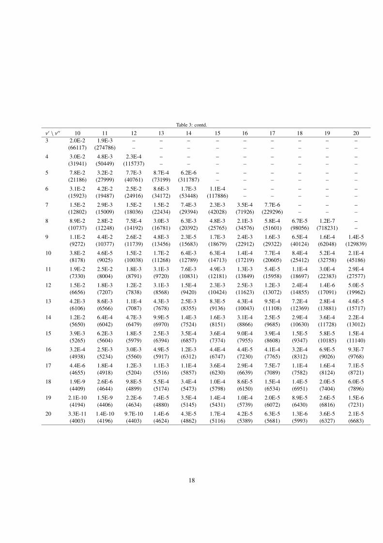
Table 3: contd.
ν′ \ ν′′ 10 11 12 13 14 15 16 17 18 19 203 2.0E-2 1.9E-3 – – – – – – – – –
(66117) (274786) – – – – – – – – –
4 3.0E-2 4.8E-3 2.3E-4 – – – – – – – –(31941) (50449) (115737) – – – – – – – –
5 7.8E-2 3.2E-2 7.7E-3 8.7E-4 6.2E-6 – – – – – –(21186) (27999) (40761) (73199) (311787) – – – – – –
6 3.1E-2 4.2E-2 2.5E-2 8.6E-3 1.7E-3 1.1E-4 – – – – –(15923) (19487) (24916) (34172) (53448) (117886) – – – – –
7 1.5E-2 2.9E-3 1.5E-2 1.5E-2 7.4E-3 2.3E-3 3.5E-4 7.7E-6 – – –(12802) (15009) (18036) (22434) (29394) (42028) (71926) (229296) – – –
8 8.9E-2 2.8E-2 7.5E-4 3.0E-3 6.3E-3 4.8E-3 2.1E-3 5.8E-4 6.7E-5 1.2E-7 –(10737) (12248) (14192) (16781) (20392) (25765) (34576) (51601) (98056) (718231) –
9 1.1E-2 4.4E-2 2.6E-2 4.8E-3 2.3E-5 1.7E-3 2.4E-3 1.6E-3 6.5E-4 1.6E-4 1.4E-5(9272) (10377) (11739) (13456) (15683) (18679) (22912) (29322) (40124) (62048) (129839)
10 3.8E-2 4.6E-5 1.5E-2 1.7E-2 6.4E-3 6.3E-4 1.4E-4 7.7E-4 8.4E-4 5.2E-4 2.1E-4(8178) (9025) (10038) (11268) (12789) (14713) (17219) (20605) (25412) (32758) (45186)
11 1.9E-2 2.5E-2 1.8E-3 3.1E-3 7.6E-3 4.9E-3 1.3E-3 5.4E-5 1.1E-4 3.0E-4 2.9E-4(7330) (8004) (8791) (9720) (10831) (12181) (13849) (15958) (18697) (22383) (27577)
12 1.5E-2 1.8E-3 1.2E-2 3.1E-3 1.5E-4 2.3E-3 2.5E-3 1.2E-3 2.4E-4 1.4E-6 5.0E-5(6656) (7207) (7838) (8568) (9420) (10424) (11623) (13072) (14855) (17091) (19962)
13 4.2E-3 8.6E-3 1.1E-4 4.3E-3 2.5E-3 8.3E-5 4.3E-4 9.5E-4 7.2E-4 2.8E-4 4.6E-5(6106) (6566) (7087) (7678) (8355) (9136) (10043) (11108) (12369) (13881) (15717)
14 1.2E-2 6.4E-4 4.7E-3 9.9E-5 1.4E-3 1.6E-3 3.1E-4 2.5E-5 2.9E-4 3.6E-4 2.2E-4(5650) (6042) (6479) (6970) (7524) (8151) (8866) (9685) (10630) (11728) (13012)
15 3.9E-3 6.2E-3 1.8E-5 2.5E-3 3.5E-4 3.6E-4 9.0E-4 3.9E-4 1.5E-5 5.8E-5 1.5E-4(5265) (5604) (5979) (6394) (6857) (7374) (7955) (8608) (9347) (10185) (11140)
16 3.2E-4 2.5E-3 3.0E-3 4.9E-5 1.2E-3 4.4E-4 4.4E-5 4.1E-4 3.2E-4 6.9E-5 9.3E-7(4938) (5234) (5560) (5917) (6312) (6747) (7230) (7765) (8312) (9026) (9768)
17 4.4E-6 1.8E-4 1.2E-3 1.1E-3 1.1E-4 3.6E-4 2.9E-4 7.5E-7 1.1E-4 1.6E-4 7.1E-5(4655) (4918) (5204) (5516) (5857) (6230) (6639) (7089) (7582) (8124) (8721)
18 1.9E-9 2.6E-6 9.8E-5 5.5E-4 3.4E-4 1.0E-4 8.6E-5 1.5E-4 1.4E-5 2.0E-5 6.0E-5(4409) (4644) (4899) (5174) (5473) (5798) (6150) (6534) (6951) (7404) (7896)
19 2.1E-10 1.5E-9 2.2E-6 7.4E-5 3.5E-4 1.4E-4 1.0E-4 2.0E-5 8.9E-5 2.6E-5 1.5E-6(4194) (4406) (4634) (4880) (5145) (5431) (5739) (6072) (6430) (6816) (7231)
20 3.3E-11 1.4E-10 9.7E-10 1.4E-6 4.3E-5 1.7E-4 4.2E-5 6.3E-5 1.3E-6 3.6E-5 2.1E-5(4003) (4196) (4403) (4624) (4862) (5116) (5389) (5681) (5993) (6327) (6683)
18
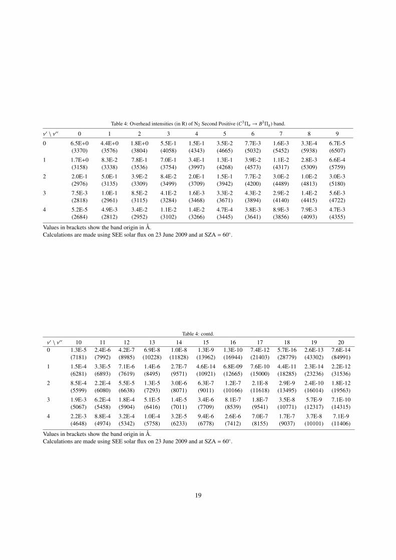
Table 4: Overhead intensities (in R) of N2 Second Positive (C3Πu → B3Πg) band.
ν′ \ ν′′ 0 1 2 3 4 5 6 7 8 9
0 6.5E+0 4.4E+0 1.8E+0 5.5E-1 1.5E-1 3.5E-2 7.7E-3 1.6E-3 3.3E-4 6.7E-5(3370) (3576) (3804) (4058) (4343) (4665) (5032) (5452) (5938) (6507)
1 1.7E+0 8.3E-2 7.8E-1 7.0E-1 3.4E-1 1.3E-1 3.9E-2 1.1E-2 2.8E-3 6.6E-4(3158) (3338) (3536) (3754) (3997) (4268) (4573) (4317) (5309) (5759)
2 2.0E-1 5.0E-1 3.9E-2 8.4E-2 2.0E-1 1.5E-1 7.7E-2 3.0E-2 1.0E-2 3.0E-3(2976) (3135) (3309) (3499) (3709) (3942) (4200) (4489) (4813) (5180)
3 7.5E-3 1.0E-1 8.5E-2 4.1E-2 1.6E-3 3.3E-2 4.3E-2 2.9E-2 1.4E-2 5.6E-3(2818) (2961) (3115) (3284) (3468) (3671) (3894) (4140) (4415) (4722)
4 5.2E-5 4.9E-3 3.4E-2 1.1E-2 1.4E-2 4.7E-4 3.8E-3 8.9E-3 7.9E-3 4.7E-3(2684) (2812) (2952) (3102) (3266) (3445) (3641) (3856) (4093) (4355)
Values in brackets show the band origin in Å.Calculations are made using SEE solar flux on 23 June 2009 and at SZA = 60◦.
Table 4: contd.
ν′ \ ν′′ 10 11 12 13 14 15 16 17 18 19 200 1.3E-5 2.4E-6 4.2E-7 6.9E-8 1.0E-8 1.3E-9 1.3E-10 7.4E-12 5.7E-16 2.6E-13 7.6E-14
(7181) (7992) (8985) (10228) (11828) (13962) (16944) (21403) (28779) (43302) (84991)
1 1.5E-4 3.3E-5 7.1E-6 1.4E-6 2.7E-7 4.6E-14 6.8E-09 7.6E-10 4.4E-11 2.3E-14 2.2E-12(6281) (6893) (7619) (8495) (9571) (10921) (12665) (15000) (18285) (23236) (31536)
2 8.5E-4 2.2E-4 5.5E-5 1.3E-5 3.0E-6 6.3E-7 1.2E-7 2.1E-8 2.9E-9 2.4E-10 1.8E-12(5599) (6080) (6638) (7293) (8071) (9011) (10166) (11618) (13495) (16014) (19563)
3 1.9E-3 6.2E-4 1.8E-4 5.1E-5 1.4E-5 3.4E-6 8.1E-7 1.8E-7 3.5E-8 5.7E-9 7.1E-10(5067) (5458) (5904) (6416) (7011) (7709) (8539) (9541) (10771) (12317) (14315)
4 2.2E-3 8.8E-4 3.2E-4 1.0E-4 3.2E-5 9.4E-6 2.6E-6 7.0E-7 1.7E-7 3.7E-8 7.1E-9(4648) (4974) (5342) (5758) (6233) (6778) (7412) (8155) (9037) (10101) (11406)
Values in brackets show the band origin in Å.Calculations are made using SEE solar flux on 23 June 2009 and at SZA = 60◦.
19
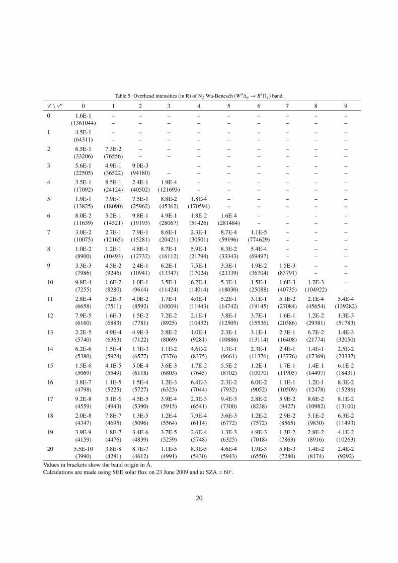
Table 5: Overhead intensities (in R) of N2 Wu-Benesch (W3∆u → B3Πg) band.
ν′ \ ν′′ 0 1 2 3 4 5 6 7 8 9
0 1.6E-1 – – – – – – – – –(1361044) – – – – – – – – –
1 4.5E-1 – – – – – – – – –(64311) – – – – – – – – –
2 6.5E-1 7.3E-2 – – – – – – – –(33206) (76556) – – – – – – – –
3 5.6E-1 4.9E-1 9.0E-3 – – – – – –(22505) (36522) (94180) – – – – – – –
4 3.5E-1 8.5E-1 2.4E-1 1.9E-4 – – – – – –(17092) (24124) (40502) (121693) – – – – – –
5 1.9E-1 7.9E-1 7.5E-1 8.8E-2 1.8E-4 – – – – –(13825) (18090) (25962) (45362) (170594) – – – – –
6 8.0E-2 5.2E-1 9.8E-1 4.9E-1 1.8E-2 1.6E-4 – – – –(11639) (14521) (19193) (28067) (51426) (281484) – – – –
7 3.0E-2 2.7E-1 7.9E-1 8.6E-1 2.3E-1 8.7E-4 1.1E-5 – – –(10075) (12165) (15281) (20421) (30501) (59196) (774629) – – –
8 1.0E-2 1.2E-1 4.8E-1 8.7E-1 5.9E-1 8.3E-2 5.4E-4 – – –(8900) (10493) (12732) (16112) (21794) (33343) (69497) – – –
9 3.3E-3 4.5E-2 2.4E-1 6.2E-1 7.5E-1 3.3E-1 1.9E-2 1.5E-3 – –(7986) (9246) (10941) (13347) (17024) (23339) (36704) (83791) – –
10 9.8E-4 1.6E-2 1.0E-1 3.5E-1 6.2E-1 5.3E-1 1.5E-1 1.6E-3 1.2E-3 –(7255) (8280) (9614) (11424) (14014) (18030) (25088) (40735) (104922) –
11 2.8E-4 5.2E-3 4.0E-2 1.7E-1 4.0E-1 5.2E-1 3.1E-1 5.1E-2 2.1E-4 5.4E-4(6658) (7511) (8592) (10009) (11943) (14742) (19145) (27084) (45654) (139282)
12 7.9E-5 1.6E-3 1.5E-2 7.2E-2 2.1E-1 3.8E-1 3.7E-1 1.6E-1 1.2E-2 1.3E-3(6160) (6883) (7781) (8925) (10432) (12505) (15536) (20386) (29381) (51783)
13 2.2E-5 4.9E-4 4.9E-3 2.8E-2 1.0E-1 2.3E-1 3.1E-1 2.3E-1 6.7E-2 1.4E-3(5740) (6363) (7122) (8069) (9281) (10886) (13114) (16408) (21774) (32050)
14 6.2E-6 1.5E-4 1.7E-3 1.1E-2 4.6E-2 1.3E-1 2.3E-1 2.4E-1 1.4E-1 2.5E-2(5380) (5924) (6577) (7376) (8375) (9661) (11376) (13776) (17369) (23337)
15 1.5E-6 4.1E-5 5.0E-4 3.6E-3 1.7E-2 5.5E-2 1.2E-1 1.7E-1 1.4E-1 6.1E-2(5069) (5549) (6118) (6803) (7645) (8702) (10070) (11905) (14497) (18431)
16 3.8E-7 1.1E-5 1.5E-4 1.2E-3 6.4E-3 2.3E-2 6.0E-2 1.1E-1 1.2E-1 8.3E-2(4798) (5225) (5727) (6323) (7044) (7932) (9052) (10509) (12478) (15286)
17 9.2E-8 3.1E-6 4.5E-5 3.9E-4 2.3E-3 9.4E-3 2.8E-2 5.9E-2 8.6E-2 8.1E-2(4559) (4943) (5390) (5915) (6541) (7300) (8238) (9427) (10982) (13100)
18 2.0E-8 7.8E-7 1.3E-5 1.2E-4 7.9E-4 3.6E-3 1.2E-2 2.9E-2 5.1E-2 6.3E-2(4347) (4695) (5096) (5564) (6114) (6772) (7572) (8565) (9830) (11493)
19 3.9E-9 1.8E-7 3.4E-6 3.7E-5 2.6E-4 1.3E-3 4.9E-3 1.3E-2 2.8E-2 4.1E-2(4159) (4476) (4839) (5259) (5748) (6325) (7018) (7863) (8916) (10263)
20 5.5E-10 3.8E-8 8.7E-7 1.1E-5 8.3E-5 4.6E-4 1.9E-3 5.8E-3 1.4E-2 2.4E-2(3990) (4281) (4612) (4991) (5430) (5943) (6550) (7280) (8174) (9292)
Values in brackets show the band origin in Å.Calculations are made using SEE solar flux on 23 June 2009 and at SZA = 60◦.
20
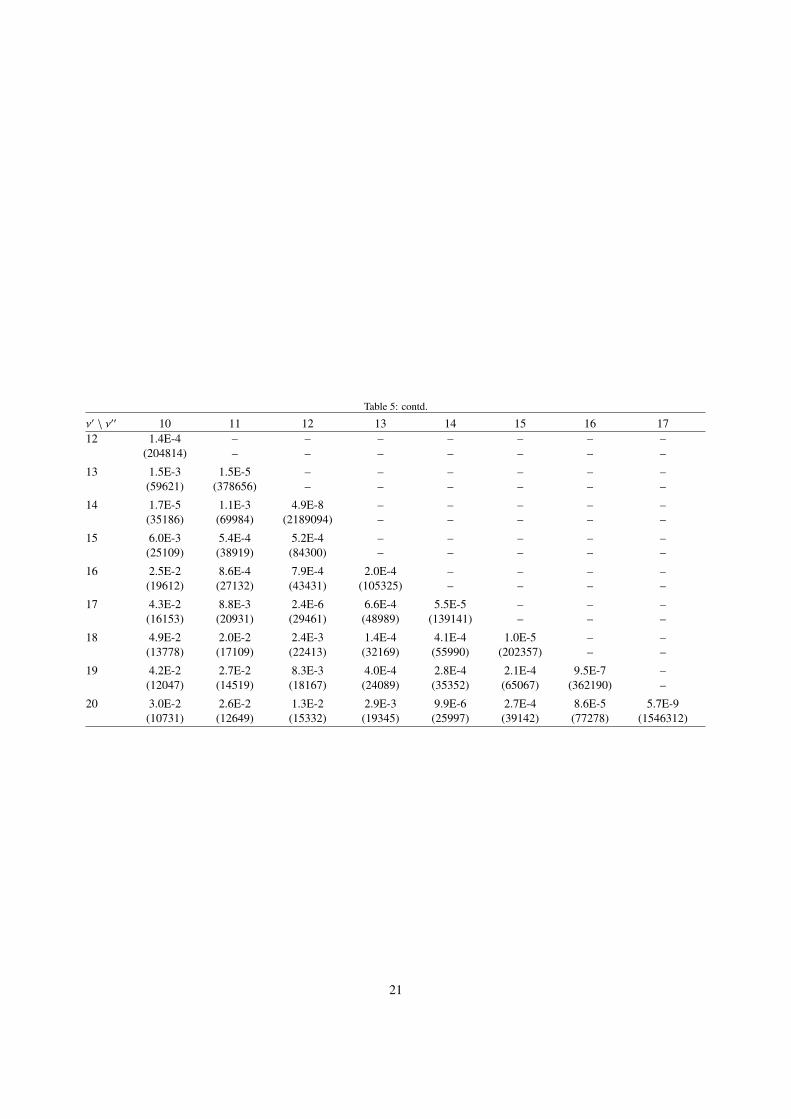
Table 5: contd.
ν′ \ ν′′ 10 11 12 13 14 15 16 1712 1.4E-4 – – – – – – –
(204814) – – – – – – –
13 1.5E-3 1.5E-5 – – – – – –(59621) (378656) – – – – – –
14 1.7E-5 1.1E-3 4.9E-8 – – – – –(35186) (69984) (2189094) – – – – –
15 6.0E-3 5.4E-4 5.2E-4 – – – – –(25109) (38919) (84300) – – – – –
16 2.5E-2 8.6E-4 7.9E-4 2.0E-4 – – – –(19612) (27132) (43431) (105325) – – – –
17 4.3E-2 8.8E-3 2.4E-6 6.6E-4 5.5E-5 – – –(16153) (20931) (29461) (48989) (139141) – – –
18 4.9E-2 2.0E-2 2.4E-3 1.4E-4 4.1E-4 1.0E-5 – –(13778) (17109) (22413) (32169) (55990) (202357) – –
19 4.2E-2 2.7E-2 8.3E-3 4.0E-4 2.8E-4 2.1E-4 9.5E-7 –(12047) (14519) (18167) (24089) (35352) (65067) (362190) –
20 3.0E-2 2.6E-2 1.3E-2 2.9E-3 9.9E-6 2.7E-4 8.6E-5 5.7E-9(10731) (12649) (15332) (19345) (25997) (39142) (77278) (1546312)
21
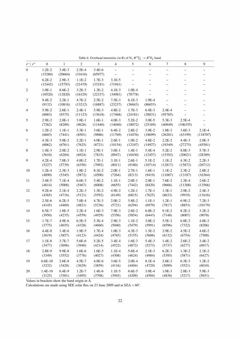
Table 6: Overhead intensities (in R) of N2 B′3Σ−u → B3Πg band.
ν′ \ ν′′ 0 1 2 3 4 5 6 7 8 9
0 1.2E-2 3.4E-3 2.5E-4 3.4E-6 – – – – – –(15280) (20664) (31616) (65977) – – – – – –
1 6.2E-2 2.9E-3 1.1E-2 1.7E-3 3.1E-5 – – – – –(12442) (15793) (21479) (33241) (71941) – – – – –
2 1.0E-1 8.6E-2 3.2E-3 1.3E-2 4.1E-3 1.0E-4 – – – –(10520) (12820) (16329) (22337) (34981) (78778) – – – –
3 9.4E-2 2.2E-1 4.7E-2 2.5E-2 7.5E-3 6.1E-3 1.9E-4 – – –(9132) (10816) (13212) (16887) (23237) (36843) (86653) – – –
4 5.9E-2 2.6E-1 2.4E-1 5.9E-3 4.8E-2 1.7E-3 6.4E-3 2.4E-4 – –(8083) (9375) (11123) (13618) (17468) (24181) (38831) (95765) – –
5 2.9E-2 2.0E-1 3.8E-1 1.6E-1 4.0E-3 5.2E-2 3.0E-5 5.3E-3 2.5E-4 –(7262) (8289) (9626) (11440) (14040) (18072) (25169) (40949) (106355) –
6 1.2E-2 1.1E-1 3.3E-1 3.6E-1 6.4E-2 2.8E-2 3.9E-2 1.8E-3 3.6E-3 2.1E-4(6603) (7441) (8501) (9886) (11769) (14476) (18699) (26201) (43199) (118707)
7 4.3E-3 5.0E-2 2.2E-1 4.0E-1 2.6E-1 1.0E-2 4.8E-2 2.2E-2 4.4E-3 2.0E-3(6062) (6761) (7625) (8721) (10154) (12107) (14927) (19349) (27275) (45581)
8 1.4E-3 2.0E-2 1.1E-1 2.9E-1 3.6E-1 1.4E-1 5.4E-4 5.2E-2 8.8E-3 5.7E-3(5610) (6204) (6924) (7815) (8947) (10430) (12457) (15392) (20021) (28389)
9 4.2E-4 7.0E-3 4.8E-2 1.7E-1 3.1E-1 2.6E-1 5.1E-2 1.1E-2 4.3E-2 2.2E-3(5227) (5739) (6350) (7092) (8011) (9180) (10714) (12817) (15872) (20712)
10 1.2E-4 2.3E-3 1.8E-2 8.1E-2 2.0E-1 2.7E-1 1.6E-1 1.1E-2 2.3E-2 2.8E-2(4890) (5345) (5872) (4500) (7264) (8213) (9419) (11007) (13187) (16364)
11 3.4E-5 7.1E-4 6.6E-3 3.4E-2 1.1E-1 2.0E-1 2.0E-1 7.6E-2 1.3E-4 2.6E-2(4614) (5008) (5467) (6008) (6655) (7442) (8420) (9666) (11308) (13566)
12 9.2E-6 2.1E-4 2.2E-3 1.3E-2 4.9E-2 1.2E-1 1.7E-1 1.3E-1 2.9E-2 2.4E-3(4365) (4716) (5121) (5592) (6149) (6815) (7625) (8633) (9919) (11616)
13 2.5E-6 6.2E-5 7.0E-4 4.7E-3 2.0E-2 5.8E-2 1.1E-1 1.2E-1 6.9E-2 7.2E-3(4145) (4460) (4821) (5236) (5721) (6294) (6979) (7817) (8853) (10179)
14 6.5E-7 1.8E-5 2.2E-4 1.6E-3 7.9E-3 2.6E-2 6.0E-2 9.1E-2 8.2E-2 3.2E-2(3950) (4235) (4559) (4929) (5356) (5854) (6443) (7148) (8007) (9078)
15 1.7E-7 4.9E-6 6.5E-5 5.3E-4 2.9E-3 1.1E-2 3.0E-2 5.5E-2 6.8E-2 4.8E-2(3775) (4035) (4328) (4660) (5040) (5479) (5991) (6596) (7322) (8206)
16 4.4E-8 1.4E-6 1.9E-5 1.7E-4 1.0E-3 4.3E-3 1.3E-2 2.9E-2 4.5E-2 4.6E-2(3619) (3857) (4123) (4424) (4765) (5155) (5606) (6132) (6754) (7500)
17 1.1E-8 3.7E-7 5.6E-6 5.2E-5 3.4E-4 1.6E-3 5.4E-3 1.4E-2 2.6E-2 3.4E-2(3477) (3696) (3940) (4214) (4522) (4872) (5273) (5737) (6277) (6917)
18 2.8E-9 9.9E-8 1.6E-6 1.6E-5 1.1E-4 5.6E-4 2.1E-3 6.2E-3 1.3E-2 2.1E-2(3349) (3552) (3776) (4027) (4308) (4624) (4984) (5395) (5871) (6427)
19 6.6E-10 2.6E-8 4.5E-7 4.8E-6 3.6E-5 2.0E-4 8.1E-4 2.6E-3 6.3E-3 1.2E-2(3232) (3420) (3629) (3859) (4116) (4404) (4729) (5099) (5521) (6010)
20 1.4E-10 6.4E-9 1.2E-7 1.4E-6 1.1E-5 6.6E-5 3.0E-4 1.0E-3 2.8E-3 5.9E-3(3125) (3301) (3495) (3708) (3945) (4209) (4504) (4838) (5217) (5651)
Values in brackets show the band origin in Å.Calculations are made using SEE solar flux on 23 June 2009 and at SZA = 60◦.
22
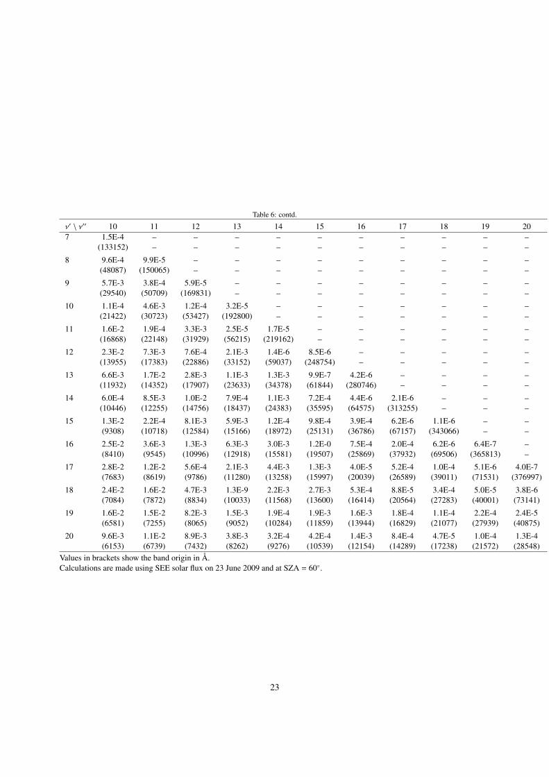
Table 6: contd.
ν′ \ ν′′ 10 11 12 13 14 15 16 17 18 19 207 1.5E-4 – – – – – – – – – –
(133152) – – – – – – – – – –
8 9.6E-4 9.9E-5 – – – – – – – – –(48087) (150065) – – – – – – – – –
9 5.7E-3 3.8E-4 5.9E-5 – – – – – – – –(29540) (50709) (169831) – – – – – – – –
10 1.1E-4 4.6E-3 1.2E-4 3.2E-5 – – – – – – –(21422) (30723) (53427) (192800) – – – – – – –
11 1.6E-2 1.9E-4 3.3E-3 2.5E-5 1.7E-5 – – – – – –(16868) (22148) (31929) (56215) (219162) – – – – – –
12 2.3E-2 7.3E-3 7.6E-4 2.1E-3 1.4E-6 8.5E-6 – – – – –(13955) (17383) (22886) (33152) (59037) (248754) – – – – –
13 6.6E-3 1.7E-2 2.8E-3 1.1E-3 1.3E-3 9.9E-7 4.2E-6 – – – –(11932) (14352) (17907) (23633) (34378) (61844) (280746) – – – –
14 6.0E-4 8.5E-3 1.0E-2 7.9E-4 1.1E-3 7.2E-4 4.4E-6 2.1E-6 – – –(10446) (12255) (14756) (18437) (24383) (35595) (64575) (313255) – – –
15 1.3E-2 2.2E-4 8.1E-3 5.9E-3 1.2E-4 9.8E-4 3.9E-4 6.2E-6 1.1E-6 – –(9308) (10718) (12584) (15166) (18972) (25131) (36786) (67157) (343066) – –
16 2.5E-2 3.6E-3 1.3E-3 6.3E-3 3.0E-3 1.2E-0 7.5E-4 2.0E-4 6.2E-6 6.4E-7 –(8410) (9545) (10996) (12918) (15581) (19507) (25869) (37932) (69506) (365813) –
17 2.8E-2 1.2E-2 5.6E-4 2.1E-3 4.4E-3 1.3E-3 4.0E-5 5.2E-4 1.0E-4 5.1E-6 4.0E-7(7683) (8619) (9786) (11280) (13258) (15997) (20039) (26589) (39011) (71531) (376997)
18 2.4E-2 1.6E-2 4.7E-3 1.3E-9 2.2E-3 2.7E-3 5.3E-4 8.8E-5 3.4E-4 5.0E-5 3.8E-6(7084) (7872) (8834) (10033) (11568) (13600) (16414) (20564) (27283) (40001) (73141)
19 1.6E-2 1.5E-2 8.2E-3 1.5E-3 1.9E-4 1.9E-3 1.6E-3 1.8E-4 1.1E-4 2.2E-4 2.4E-5(6581) (7255) (8065) (9052) (10284) (11859) (13944) (16829) (21077) (27939) (40875)
20 9.6E-3 1.1E-2 8.9E-3 3.8E-3 3.2E-4 4.2E-4 1.4E-3 8.4E-4 4.7E-5 1.0E-4 1.3E-4(6153) (6739) (7432) (8262) (9276) (10539) (12154) (14289) (17238) (21572) (28548)
Values in brackets show the band origin in Å.Calculations are made using SEE solar flux on 23 June 2009 and at SZA = 60◦.
23
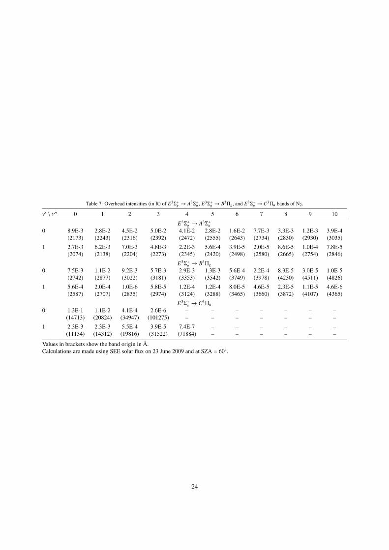
Table 7: Overhead intensities (in R) of E3Σ+g → A3Σ+
u , E3Σ+g → B3Πg, and E3Σ+
g → C3Πu bands of N2.
ν′ \ ν′′ 0 1 2 3 4 5 6 7 8 9 10
E3Σ+g → A3Σ+
u0 8.9E-3 2.8E-2 4.5E-2 5.0E-2 4.1E-2 2.8E-2 1.6E-2 7.7E-3 3.3E-3 1.2E-3 3.9E-4
(2173) (2243) (2316) (2392) (2472) (2555) (2643) (2734) (2830) (2930) (3035)
1 2.7E-3 6.2E-3 7.0E-3 4.8E-3 2.2E-3 5.6E-4 3.9E-5 2.0E-5 8.6E-5 1.0E-4 7.8E-5(2074) (2138) (2204) (2273) (2345) (2420) (2498) (2580) (2665) (2754) (2846)
E3Σ+g → B3Πg
0 7.5E-3 1.1E-2 9.2E-3 5.7E-3 2.9E-3 1.3E-3 5.6E-4 2.2E-4 8.3E-5 3.0E-5 1.0E-5(2742) (2877) (3022) (3181) (3353) (3542) (3749) (3978) (4230) (4511) (4826)
1 5.6E-4 2.0E-4 1.0E-6 5.8E-5 1.2E-4 1.2E-4 8.0E-5 4.6E-5 2.3E-5 1.1E-5 4.6E-6(2587) (2707) (2835) (2974) (3124) (3288) (3465) (3660) (3872) (4107) (4365)
E3Σ+g → C3Πu
0 1.3E-1 1.1E-2 4.1E-4 2.6E-6 – – – – – – –(14713) (20824) (34947) (101275) – – – – – – –
1 2.3E-3 2.3E-3 5.5E-4 3.9E-5 7.4E-7 – – – – – –(11134) (14312) (19816) (31522) (71884) – – – – – –
Values in brackets show the band origin in Å.Calculations are made using SEE solar flux on 23 June 2009 and at SZA = 60◦.
24
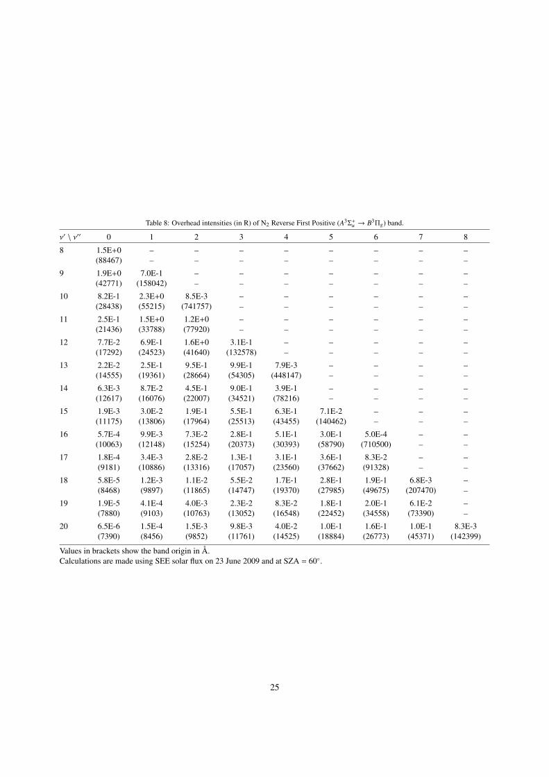
Table 8: Overhead intensities (in R) of N2 Reverse First Positive (A3Σ+u → B3Πg) band.
ν′ \ ν′′ 0 1 2 3 4 5 6 7 8
8 1.5E+0 – – – – – – – –(88467) – – – – – – – –
9 1.9E+0 7.0E-1 – – – – – – –(42771) (158042) – – – – – – –
10 8.2E-1 2.3E+0 8.5E-3 – – – – – –(28438) (55215) (741757) – – – – – –
11 2.5E-1 1.5E+0 1.2E+0 – – – – – –(21436) (33788) (77920) – – – – – –
12 7.7E-2 6.9E-1 1.6E+0 3.1E-1 – – – – –(17292) (24523) (41640) (132578) – – – – –
13 2.2E-2 2.5E-1 9.5E-1 9.9E-1 7.9E-3 – – – –(14555) (19361) (28664) (54305) (448147) – – – –
14 6.3E-3 8.7E-2 4.5E-1 9.0E-1 3.9E-1 – – – –(12617) (16076) (22007) (34521) (78216) – – – –
15 1.9E-3 3.0E-2 1.9E-1 5.5E-1 6.3E-1 7.1E-2 – – –(11175) (13806) (17964) (25513) (43455) (140462) – – –
16 5.7E-4 9.9E-3 7.3E-2 2.8E-1 5.1E-1 3.0E-1 5.0E-4 – –(10063) (12148) (15254) (20373) (30393) (58790) (710500) – –
17 1.8E-4 3.4E-3 2.8E-2 1.3E-1 3.1E-1 3.6E-1 8.3E-2 – –(9181) (10886) (13316) (17057) (23560) (37662) (91328) – –
18 5.8E-5 1.2E-3 1.1E-2 5.5E-2 1.7E-1 2.8E-1 1.9E-1 6.8E-3 –(8468) (9897) (11865) (14747) (19370) (27985) (49675) (207470) –
19 1.9E-5 4.1E-4 4.0E-3 2.3E-2 8.3E-2 1.8E-1 2.0E-1 6.1E-2 –(7880) (9103) (10763) (13052) (16548) (22452) (34558) (73390) –
20 6.5E-6 1.5E-4 1.5E-3 9.8E-3 4.0E-2 1.0E-1 1.6E-1 1.0E-1 8.3E-3(7390) (8456) (9852) (11761) (14525) (18884) (26773) (45371) (142399)
Values in brackets show the band origin in Å.Calculations are made using SEE solar flux on 23 June 2009 and at SZA = 60◦.
25