Probability review II:Random variables and dependencies

between them

Instructor: Taylor Berg-KirkpatrickSlides: Sanjoy Dasgupta

Random variables

Roll two dice. Let X be their sum.E.g.,

outcome = (1, 1) ⇒ X = 2

outcome = (1, 2) or (2, 1) ⇒ X = 3

Probability space:

• Sample space: Ω = 1, 2, 3, 4, 5, 6 × 1, 2, 3, 4, 5, 6.• Each outcome equally likely.

Random variable X lies in 2, 3, 4, 5, 6, 7, 8, 9, 10, 11, 12.

A random variable (r.v.) is a defined on a probability space.It is a mapping from Ω (outcomes) to R (numbers).We’ll use capital letters for r.v.’s.

Random variables

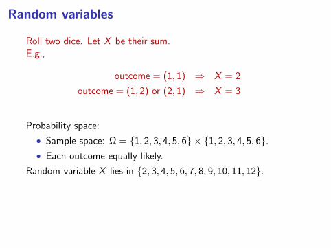
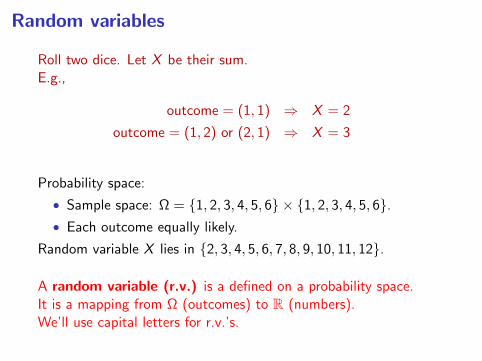
Roll two dice. Let X be their sum.E.g.,

outcome = (1, 1) ⇒ X = 2

outcome = (1, 2) or (2, 1) ⇒ X = 3

Probability space:

• Sample space: Ω = 1, 2, 3, 4, 5, 6 × 1, 2, 3, 4, 5, 6.• Each outcome equally likely.

Random variable X lies in 2, 3, 4, 5, 6, 7, 8, 9, 10, 11, 12.

A random variable (r.v.) is a defined on a probability space.It is a mapping from Ω (outcomes) to R (numbers).We’ll use capital letters for r.v.’s.

Random variables

Roll two dice. Let X be their sum.E.g.,

outcome = (1, 1) ⇒ X = 2

outcome = (1, 2) or (2, 1) ⇒ X = 3

Probability space:

• Sample space: Ω = 1, 2, 3, 4, 5, 6 × 1, 2, 3, 4, 5, 6.• Each outcome equally likely.

Random variable X lies in 2, 3, 4, 5, 6, 7, 8, 9, 10, 11, 12.

A random variable (r.v.) is a defined on a probability space.It is a mapping from Ω (outcomes) to R (numbers).We’ll use capital letters for r.v.’s.

The distribution of a random variable

Roll a die.

Define X = 1 if die is ≥ 3, otherwise X = 0.

Another example

Throw a dart at a dartboard of radius 1.

Let X = distance to center of board.

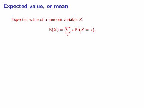
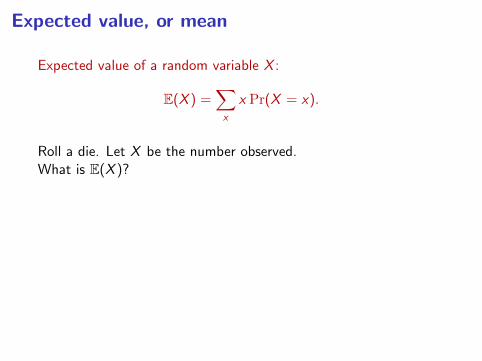
Expected value, or mean

Expected value of a random variable X :

E(X ) =∑x

x Pr(X = x).

Roll a die. Let X be the number observed.What is E(X )?

Expected value, or mean

Expected value of a random variable X :

E(X ) =∑x

x Pr(X = x).

Roll a die. Let X be the number observed.What is E(X )?

Another example

A biased coin has heads probability p.Let X be 1 if heads, 0 if tails. What is E(X )?

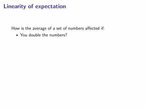
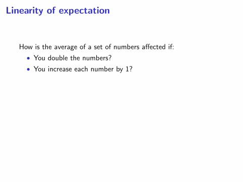
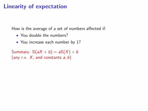
Linearity of expectation

How is the average of a set of numbers affected if:

• You double the numbers?

• You increase each number by 1?

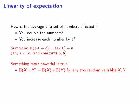
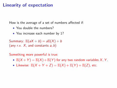
Summary: E(aX + b) = aE(X ) + b(any r.v. X , and constants a, b)

Something more powerful is true:

• E(X +Y ) = E(X ) +E(Y ) for any two random variables X ,Y .

• Likewise: E(X + Y + Z ) = E(X ) + E(Y ) + E(Z ), etc.

Linearity of expectation

How is the average of a set of numbers affected if:

• You double the numbers?

• You increase each number by 1?

Summary: E(aX + b) = aE(X ) + b(any r.v. X , and constants a, b)

Something more powerful is true:

• E(X +Y ) = E(X ) +E(Y ) for any two random variables X ,Y .

• Likewise: E(X + Y + Z ) = E(X ) + E(Y ) + E(Z ), etc.

Linearity of expectation

How is the average of a set of numbers affected if:

• You double the numbers?

• You increase each number by 1?

Summary: E(aX + b) = aE(X ) + b(any r.v. X , and constants a, b)

Something more powerful is true:

• E(X +Y ) = E(X ) +E(Y ) for any two random variables X ,Y .

• Likewise: E(X + Y + Z ) = E(X ) + E(Y ) + E(Z ), etc.

Linearity of expectation

How is the average of a set of numbers affected if:

• You double the numbers?

• You increase each number by 1?

Summary: E(aX + b) = aE(X ) + b(any r.v. X , and constants a, b)

Something more powerful is true:

• E(X +Y ) = E(X ) +E(Y ) for any two random variables X ,Y .

• Likewise: E(X + Y + Z ) = E(X ) + E(Y ) + E(Z ), etc.

Linearity of expectation

How is the average of a set of numbers affected if:

• You double the numbers?

• You increase each number by 1?

Summary: E(aX + b) = aE(X ) + b(any r.v. X , and constants a, b)

Something more powerful is true:

• E(X +Y ) = E(X ) +E(Y ) for any two random variables X ,Y .

• Likewise: E(X + Y + Z ) = E(X ) + E(Y ) + E(Z ), etc.

Linearity: examples

Roll 2 dice and let Z denote the sum. What is E(Z )?

Method 1Distribution of Z :

z 2 3 4 5 6 7 8 9 10 11 12

Pr(Z = z) 136

236

336

436

536

636

536

436

336

236

136

∴ E(Z ) = 2 · 1

36+ 3 · 2

36+ 4 · 3

36+ · · · = 7.

Method 2Let X1 be the first die and X2 the second die. Each of them is asingle die and thus (as we saw earlier) has expected value 3.5.Since Z = X1 + X2,

E(Z ) = E(X1) + E(X2) = 3.5 + 3.5 = 7.

Linearity: examples

Roll 2 dice and let Z denote the sum. What is E(Z )?

Method 1Distribution of Z :

z 2 3 4 5 6 7 8 9 10 11 12

Pr(Z = z) 136

236

336

436

536

636

536

436

336

236

136

∴ E(Z ) = 2 · 1

36+ 3 · 2

36+ 4 · 3

36+ · · · = 7.

Method 2Let X1 be the first die and X2 the second die. Each of them is asingle die and thus (as we saw earlier) has expected value 3.5.Since Z = X1 + X2,

E(Z ) = E(X1) + E(X2) = 3.5 + 3.5 = 7.

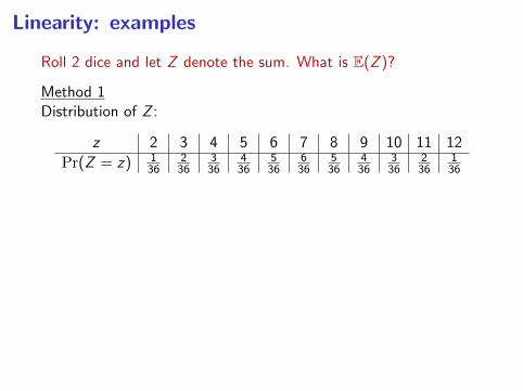
Linearity: examples

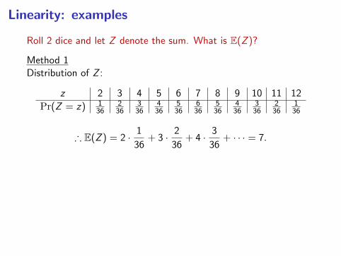
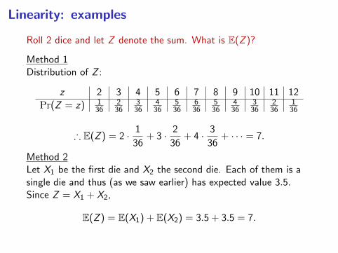
Roll 2 dice and let Z denote the sum. What is E(Z )?

Method 1Distribution of Z :

z 2 3 4 5 6 7 8 9 10 11 12

Pr(Z = z) 136

236

336

436

536

636

536

436

336

236

136

∴ E(Z ) = 2 · 1

36+ 3 · 2

36+ 4 · 3

36+ · · · = 7.

Method 2Let X1 be the first die and X2 the second die. Each of them is asingle die and thus (as we saw earlier) has expected value 3.5.Since Z = X1 + X2,

E(Z ) = E(X1) + E(X2) = 3.5 + 3.5 = 7.

Linearity: examples

Roll 2 dice and let Z denote the sum. What is E(Z )?

Method 1Distribution of Z :

z 2 3 4 5 6 7 8 9 10 11 12

Pr(Z = z) 136

236

336

436

536

636

536

436

336

236

136

∴ E(Z ) = 2 · 1

36+ 3 · 2

36+ 4 · 3

36+ · · · = 7.

Method 2Let X1 be the first die and X2 the second die. Each of them is asingle die and thus (as we saw earlier) has expected value 3.5.Since Z = X1 + X2,

E(Z ) = E(X1) + E(X2) = 3.5 + 3.5 = 7.

Another example

Toss n coins of bias p.Let X be the number of heads.What is E(X )?

Variance

Can summarize an r.v. X by the mean/median, µ.

But these don’t capture the spread of X :

x

Pr(x)

x

Pr(x)

µ µ

A measure of spread: average distance from the mean, E(|X −µ|)?

• Variance: var(X ) = E(X − µ)2, where µ = E(X )

• Standard deviation√

var(X ): roughly, the average amountby which X differs from its mean.

Variance

Can summarize an r.v. X by the mean/median, µ.

But these don’t capture the spread of X :

x

Pr(x)

x

Pr(x)

µ µ

A measure of spread: average distance from the mean, E(|X −µ|)?

• Variance: var(X ) = E(X − µ)2, where µ = E(X )

• Standard deviation√

var(X ): roughly, the average amountby which X differs from its mean.

Variance

Can summarize an r.v. X by the mean/median, µ.

But these don’t capture the spread of X :

x

Pr(x)

x

Pr(x)

µ µ

A measure of spread: average distance from the mean, E(|X −µ|)?

• Variance: var(X ) = E(X − µ)2, where µ = E(X )

• Standard deviation√

var(X ): roughly, the average amountby which X differs from its mean.

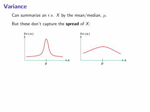
Variance

Can summarize an r.v. X by the mean/median, µ.

But these don’t capture the spread of X :

x

Pr(x)

x

Pr(x)

µ µ

A measure of spread: average distance from the mean, E(|X −µ|)?

• Variance: var(X ) = E(X − µ)2, where µ = E(X )

• Standard deviation√

var(X ): roughly, the average amountby which X differs from its mean.

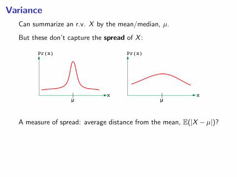
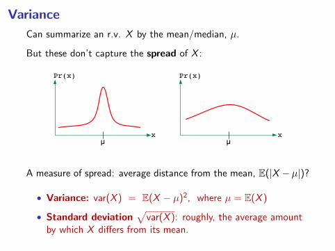
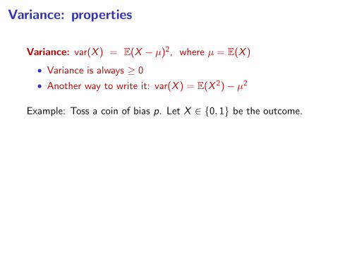
Variance: properties

Variance: var(X ) = E(X − µ)2, where µ = E(X )

• Variance is always ≥ 0

• Another way to write it: var(X ) = E(X 2)− µ2

Example: Toss a coin of bias p. Let X ∈ 0, 1 be the outcome.

Variance: properties

Variance: var(X ) = E(X − µ)2, where µ = E(X )

• Variance is always ≥ 0

• Another way to write it: var(X ) = E(X 2)− µ2

Example: Toss a coin of bias p. Let X ∈ 0, 1 be the outcome.

Independent random variables

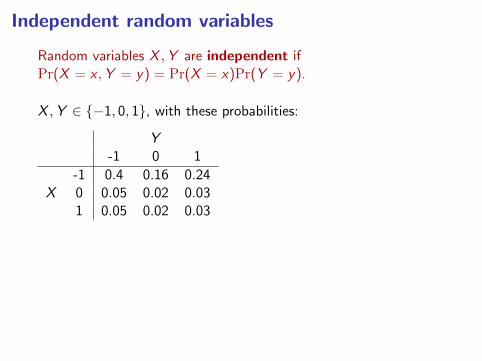
Random variables X ,Y are independent ifPr(X = x ,Y = y) = Pr(X = x)Pr(Y = y).

Pick a card out of a standard deck.X = suit and Y = number.

Independent random variables

Random variables X ,Y are independent ifPr(X = x ,Y = y) = Pr(X = x)Pr(Y = y).

Pick a card out of a standard deck.X = suit and Y = number.

Independent random variables

Random variables X ,Y are independent ifPr(X = x ,Y = y) = Pr(X = x)Pr(Y = y).

Flip a fair coin 10 times.X = # heads and Y = last toss.

Independent random variables

Random variables X ,Y are independent ifPr(X = x ,Y = y) = Pr(X = x)Pr(Y = y).

X ,Y ∈ −1, 0, 1, with these probabilities:

Y-1 0 1

-1 0.4 0.16 0.24X 0 0.05 0.02 0.03

1 0.05 0.02 0.03

Dependence

Example: Pick a person at random, and take

H = height

W = weight

Independence would mean

Pr(H = h,W = w) = Pr(H = h)Pr(W = w).

Not accurate: height and weight will be positively correlated.

Dependence

Example: Pick a person at random, and take

H = height

W = weight

Independence would mean

Pr(H = h,W = w) = Pr(H = h)Pr(W = w).

Not accurate: height and weight will be positively correlated.

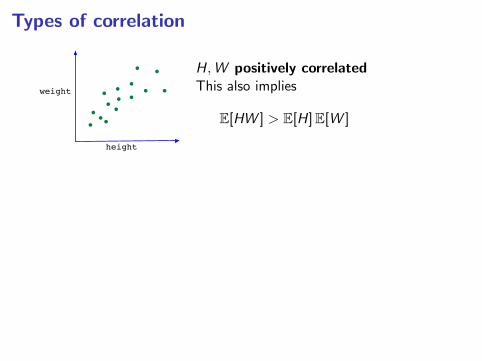
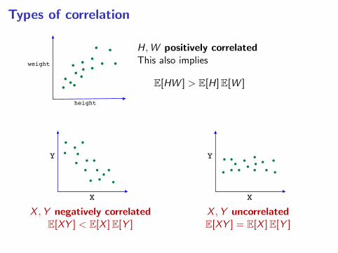
Types of correlation

height

weight

H,W positively correlatedThis also implies

E[HW ] > E[H]E[W ]

Y

X

X ,Y negatively correlatedE[XY ] < E[X ]E[Y ]

Y

X

X ,Y uncorrelatedE[XY ] = E[X ]E[Y ]

Types of correlation

height

weight

H,W positively correlatedThis also implies

E[HW ] > E[H]E[W ]

Y

X

X ,Y negatively correlatedE[XY ] < E[X ]E[Y ]

Y

X

X ,Y uncorrelatedE[XY ] = E[X ]E[Y ]

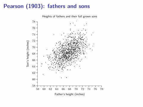
Pearson (1903): fathers and sons

PEARSON’S FATHER-SON DATA

• The following scatter diagram shows the heights of 1,078fathers and their full-grown sons, in England, circa 1900.There is one dot for each father-son pair.

58 60 62 64 66 68 70 72 74 76 78

Father’s height (inches)

58

60

62

64

66

68

70

72

74

76

78

Son

’shei

ght

(inch

es)

Heights of fathers and their full grown sons

• How would you describe the relationship between the heightsof the fathers and the heights of their sons?

• For a father of a given height, what height would you predictfor his son?

10–1

• How tall are the sons of 6 foot fathers?

58 60 62 64 66 68 70 72 74 76 78

Father’s height (inches)

58

60

62

64

66

68

70

72

74

76

78

Son

’shei

ght

(inch

es)

Father-son pairs where the father is 6 feet tall

£

• The points in the vertical chimney are the father-son pairswhere the father is 6 feet tall, to the nearest inch.

• The cross marks the average height of the sons of thesefathers.

• These sons are inches tall, on average.

• This is the natural guess for the height of a son of a 6foot father.

10–2

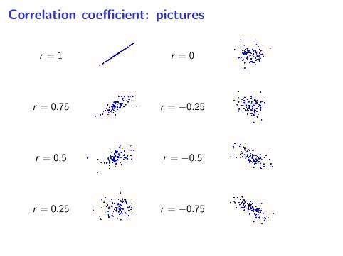
Correlation coefficient: pictures

r = 1 r = 0

r = 0.75 r = −0.25

r = 0.5 r = −0.5

r = 0.25 r = −0.75

Covariance and correlation

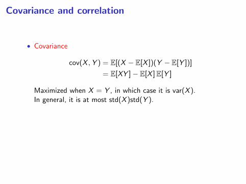
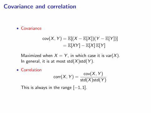
• Covariance

cov(X ,Y ) = E[(X − E[X ])(Y − E[Y ])]

= E[XY ]− E[X ]E[Y ]

Maximized when X = Y , in which case it is var(X ).In general, it is at most std(X )std(Y ).

• Correlation

corr(X ,Y ) =cov(X ,Y )

std(X )std(Y )

This is always in the range [−1, 1].

Covariance and correlation

• Covariance

cov(X ,Y ) = E[(X − E[X ])(Y − E[Y ])]

= E[XY ]− E[X ]E[Y ]

Maximized when X = Y , in which case it is var(X ).In general, it is at most std(X )std(Y ).

• Correlation

corr(X ,Y ) =cov(X ,Y )

std(X )std(Y )

This is always in the range [−1, 1].

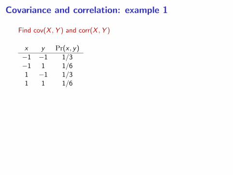
Covariance and correlation: example 1

Find cov(X ,Y ) and corr(X ,Y )

x y Pr(x , y)

−1 −1 1/3−1 1 1/61 −1 1/31 1 1/6

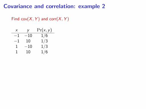
Covariance and correlation: example 2

Find cov(X ,Y ) and corr(X ,Y )

x y Pr(x , y)

−1 −10 1/6−1 10 1/31 −10 1/31 10 1/6