
Probability - Pomona Collegepages.pomona.edu/~ajr04747/Fall2016/Math151/Notes/Math...Chapter 1...
146
Probability Lecture Notes Adolfo J. Rumbos c Draft date: November 6, 2016 November 6, 2016
Transcript of Probability - Pomona Collegepages.pomona.edu/~ajr04747/Fall2016/Math151/Notes/Math...Chapter 1...

Probability
Lecture Notes
Adolfo J. Rumbosc© Draft date: November 6, 2016
November 6, 2016

2
Contents
1 Preface 5
2 Introduction: An example from statistical inference 7
3 Probability Spaces 11
3.1 Sample Spaces and σ–fields . . . . . . . . . . . . . . . . . . . . . 11
3.2 Some Set Algebra . . . . . . . . . . . . . . . . . . . . . . . . . . . 13
3.3 More on σ–fields . . . . . . . . . . . . . . . . . . . . . . . . . . . 16
3.4 Defining a Probability Function . . . . . . . . . . . . . . . . . . . 20
3.4.1 Properties of Probability Spaces . . . . . . . . . . . . . . 20
3.4.2 Constructing Probability Functions . . . . . . . . . . . . . 26
3.5 Independent Events . . . . . . . . . . . . . . . . . . . . . . . . . 28
3.6 Conditional Probability . . . . . . . . . . . . . . . . . . . . . . . 30
3.6.1 Some Properties of Conditional Probabilities . . . . . . . 32
4 Random Variables 37
4.1 Definition of Random Variable . . . . . . . . . . . . . . . . . . . 37
4.2 Distribution Functions . . . . . . . . . . . . . . . . . . . . . . . 38
5 Expectation of Random Variables 47
5.1 Expected Value of a Random Variable . . . . . . . . . . . . . . . 47
5.2 Properties of Expectations . . . . . . . . . . . . . . . . . . . . . . 59
5.2.1 Linearity . . . . . . . . . . . . . . . . . . . . . . . . . . . 59
5.2.2 Expectations of Functions of Random Variables . . . . . . 60
5.3 Moments . . . . . . . . . . . . . . . . . . . . . . . . . . . . . . . 62
5.3.1 Moment Generating Function . . . . . . . . . . . . . . . . 63
5.3.2 Properties of Moment Generating Functions . . . . . . . . 65
5.4 Variance . . . . . . . . . . . . . . . . . . . . . . . . . . . . . . . . 69
6 Joint Distributions 71
6.1 Definition of Joint Distribution . . . . . . . . . . . . . . . . . . . 71
6.2 Marginal Distributions . . . . . . . . . . . . . . . . . . . . . . . . 75
6.3 Independent Random Variables . . . . . . . . . . . . . . . . . . . 78
3

4 CONTENTS
7 Some Special Distributions 917.1 The Normal Distribution . . . . . . . . . . . . . . . . . . . . . . . 917.2 The Poisson Distribution . . . . . . . . . . . . . . . . . . . . . . 96
8 Convergence in Distribution 1018.1 Definition of Convergence in Distribution . . . . . . . . . . . . . 1018.2 mgf Convergence Theorem . . . . . . . . . . . . . . . . . . . . . . 1028.3 Central Limit Theorem . . . . . . . . . . . . . . . . . . . . . . . 110
9 Introduction to Estimation 1159.1 Point Estimation . . . . . . . . . . . . . . . . . . . . . . . . . . . 1159.2 Estimating the Mean . . . . . . . . . . . . . . . . . . . . . . . . . 1179.3 Estimating Proportions . . . . . . . . . . . . . . . . . . . . . . . 1199.4 Interval Estimates for the Mean . . . . . . . . . . . . . . . . . . . 121
9.4.1 The χ2 Distribution . . . . . . . . . . . . . . . . . . . . . 1239.4.2 The t Distribution . . . . . . . . . . . . . . . . . . . . . . 1309.4.3 Sampling from a normal distribution . . . . . . . . . . . . 1339.4.4 Distribution of the Sample Variance from a Normal Dis-
tribution . . . . . . . . . . . . . . . . . . . . . . . . . . . 1379.4.5 The Distribution of Tn . . . . . . . . . . . . . . . . . . . . 144
Chapter 1
Preface
This set of notes has been developed in conjunction with the teaching of Prob-ability at Pomona College over the course of many semesters. The main goalof the course has been to introduce the theory and practice of Probability inthe context of problems in statistical inference. Many of the students in thecourse will take a statistical inference course in a subsequent semester and willget to put into practice the theory and techniques developed in the course. Forthe rest of the students, the course is a solid introduction to Probability, whichbegins with the fundamental definitions of sample spaces, probability, randomvariables, distribution functions, and culminates with the celebrated CentralLimit Theorem and its applications. This course also serves as an introductionto probabilistic modeling and presents good preparation for subsequent coursesin mathematical modeling and stochastic processes.
5

6 CHAPTER 1. PREFACE
Chapter 2
Introduction: An examplefrom statistical inference
I had two coins: a trick coin and a fair one. The fair coin has an equal chance oflanding heads and tails after being tossed. The trick coin is rigged so that 40%of the time it comes up head. I lost one of the coins, and I don’t know whetherthe coin I have left is the trick coin, or the fair one. How do I determine whetherI have the trick coin or the fair coin?
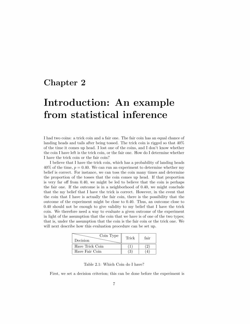
I believe that I have the trick coin, which has a probability of landing heads40% of the time, p = 0.40. We can run an experiment to determine whether mybelief is correct. For instance, we can toss the coin many times and determinethe proportion of the tosses that the coin comes up head. If that proportionis very far off from 0.40, we might be led to believe that the coin is perhapsthe fair one. If the outcome is in a neighborhood of 0.40, we might concludethat the my belief that I have the trick is correct. However, in the event thatthe coin that I have is actually the fair coin, there is the possibility that theoutcome of the experiment might be close to 0.40. Thus, an outcome close to0.40 should not be enough to give validity to my belief that I have the trickcoin. We therefore need a way to evaluate a given outcome of the experimentin light of the assumption that the coin that we have is of one of the two types;that is, under the assumption that the coin is the fair coin or the trick one. Wewill next describe how this evaluation procedure can be set up.
````````````DecisionCoin Type
Trick fair
Have Trick Coin (1) (2)Have Fair Coin (3) (4)
Table 2.1: Which Coin do I have?
First, we set a decision criterion; this can be done before the experiment is
7
8CHAPTER 2. INTRODUCTION: AN EXAMPLE FROM STATISTICAL INFERENCE
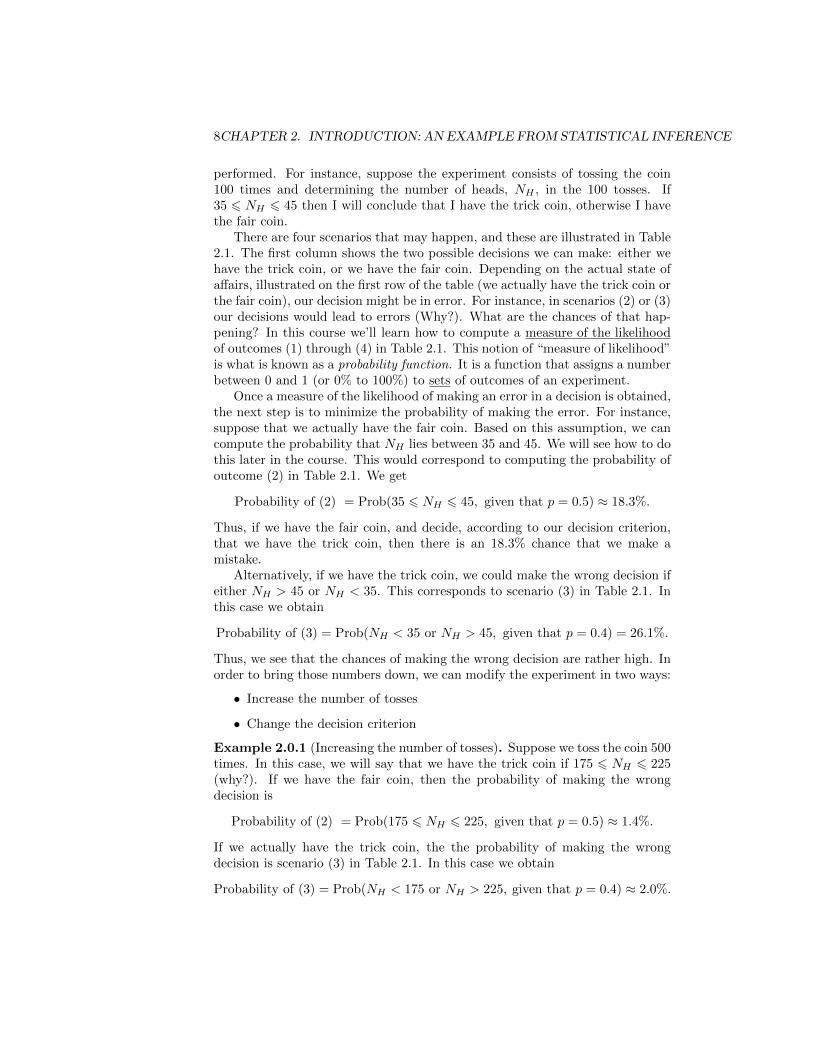
performed. For instance, suppose the experiment consists of tossing the coin100 times and determining the number of heads, NH , in the 100 tosses. If35 6 NH 6 45 then I will conclude that I have the trick coin, otherwise I havethe fair coin.
There are four scenarios that may happen, and these are illustrated in Table2.1. The first column shows the two possible decisions we can make: either wehave the trick coin, or we have the fair coin. Depending on the actual state ofaffairs, illustrated on the first row of the table (we actually have the trick coin orthe fair coin), our decision might be in error. For instance, in scenarios (2) or (3)our decisions would lead to errors (Why?). What are the chances of that hap-pening? In this course we’ll learn how to compute a measure of the likelihoodof outcomes (1) through (4) in Table 2.1. This notion of “measure of likelihood”is what is known as a probability function. It is a function that assigns a numberbetween 0 and 1 (or 0% to 100%) to sets of outcomes of an experiment.
Once a measure of the likelihood of making an error in a decision is obtained,the next step is to minimize the probability of making the error. For instance,suppose that we actually have the fair coin. Based on this assumption, we cancompute the probability that NH lies between 35 and 45. We will see how to dothis later in the course. This would correspond to computing the probability ofoutcome (2) in Table 2.1. We get
Probability of (2) = Prob(35 6 NH 6 45, given that p = 0.5) ≈ 18.3%.
Thus, if we have the fair coin, and decide, according to our decision criterion,that we have the trick coin, then there is an 18.3% chance that we make amistake.
Alternatively, if we have the trick coin, we could make the wrong decision ifeither NH > 45 or NH < 35. This corresponds to scenario (3) in Table 2.1. Inthis case we obtain
Probability of (3) = Prob(NH < 35 or NH > 45, given that p = 0.4) = 26.1%.
Thus, we see that the chances of making the wrong decision are rather high. Inorder to bring those numbers down, we can modify the experiment in two ways:
• Increase the number of tosses
• Change the decision criterion
Example 2.0.1 (Increasing the number of tosses). Suppose we toss the coin 500times. In this case, we will say that we have the trick coin if 175 6 NH 6 225(why?). If we have the fair coin, then the probability of making the wrongdecision is
Probability of (2) = Prob(175 6 NH 6 225, given that p = 0.5) ≈ 1.4%.
If we actually have the trick coin, the the probability of making the wrongdecision is scenario (3) in Table 2.1. In this case we obtain
Probability of (3) = Prob(NH < 175 or NH > 225, given that p = 0.4) ≈ 2.0%.

9
Note that in this case, the probabilities of making an error are drastically re-duced from those in the 100 tosses experiment. Thus, we would be more confi-dent in our conclusions based on our decision criteria. However, it is importantto keep in mind that there is chance, albeit small, of reaching the wrong con-clusion.
Example 2.0.2 (Change the decision criterion). Toss the coin 100 times andsuppose that we say that we have the trick coin if 37 6 NH 6 43; in otherwords, we choose a narrower decision criterion.
In this case,
Probability of (2) = Prob(37 6 NH 6 43, given that p = 0.5) ≈ 9.3%
and
Probability of (3) = Prob(NH < 37 or NH > 43, given that p = 0.4) ≈ 47.5%.
Observe that, in this case, the probability of making an error if we actually havethe fair coin is decreased in the case of the 100 tosses experiment; however, ifwe do have the trick coin, then the probability of making an error is increasedfrom that of the original setup.
Our first goal in this course is to define the notion of probability that allowedus to make the calculations presented in this example. Although we will continueto use the coin–tossing experiment as an example to illustrate various conceptsand calculations that will be introduced, the notion of probability that we willdevelop will extend beyond the coin–tossing example presented in this section.In order to define a probability function, we will first need to develop the notionof a Probability Space.

10CHAPTER 2. INTRODUCTION: AN EXAMPLE FROM STATISTICAL INFERENCE
Chapter 3
Probability Spaces
3.1 Sample Spaces and σ–fields
In this section we discuss a class of objects for which a probability functioncan be defined; these are called events. Events are sets of outcomes of randomexperiments. We shall then begin with the definition of a random experiment.The set of all possible outcomes of random experiment is called the sample spacefor the experiment; this will be the starting point from which we will build atheory of probability.
A random experiment is a process or observation that can be repeated indefi-nitely under the same conditions, and whose outcomes cannot be predicted withcertainty before the experiment is performed. For instance, if a coin is flipped100 times, the number of heads that come up cannot be determined with cer-tainty. The set of all possible outcomes of a random experiment is called thesample space of the experiment. In the case of 100 tosses of a coin, the samplespaces is the set of all possible sequences of Heads (H) and Tails (T) of length100:
H H H H . . . HT H H H . . . HH T H H . . . H...
Events are subsets of the sample space for which we can compute probabilities.If we denote the sample space for an experiment by C, a subset, E, of C, denoted
E ⊆ C,
is a collection of outcomes in C. For example, in the 100–coin–toss experiment,if we denote the number of heads in an outcome by NH ; then the set of outcomesfor which 35 6 NH 6 45 is a subset of C. We will denote this set by (35 6NH 6 45), so that
(35 6 NH 6 45) ⊆ C,
11

12 CHAPTER 3. PROBABILITY SPACES
the set of sequences of H and T that have between 35 and 45 heads.
Events are a special class of subsets of a sample space C. These subsets satisfya set of axioms known as the axioms of a σ–algebra, or the σ–field axioms.
Definition 3.1.1 (σ-field). A collection of subsets, B, of a sample space C,referred to as events, is called a σ–field if it satisfies the following properties:
1. ∅ ∈ B (∅ denotes the empty set, or the set with no elements).
2. If E ∈ B, then its complement, Ec (the set of outcomes in the samplespace that are not in E) is also an element of B; in symbols, we write
E ∈ B ⇒ Ec ∈ B.
3. If (E1, E2, E3 . . .) is a sequence of events, then the union of the events isalso in B; in symbols,
Ek ∈ B for k = 1, 2, 3, . . . ,⇒ E1 ∪ E2 ∪ E3 ∪ . . . =
∞⋃k=1
Ek ∈ B,
where
∞⋃k=1
Ek denotes the collection of outcomes in the sample space that
belong to at least one of the events Ek, for k = 1, 2, 3, . . .
Example 3.1.2. Toss a coin three times in a row. The sample space, C, forthis experiment consists of all triples of heads (H) and tails (T ):
HHHHHTHTHHTTTHHTHTTTHTTT
Sample Space
An example of a σ–field for this sample space consists of all possible subsetsof the sample space. There are 28 = 256 possible subsets of this sample space;these include the empty set ∅ and the entire sample space C.
An example of an event, E, is the the set of outcomes that yield at least onehead:
E = {HHH, HHT, HTH, HTT, THH, THT, TTH}.
Its complement, Ec, is also an event:
Ec = {TTT}.
3.2. SOME SET ALGEBRA 13
3.2 Some Set Algebra
Since a σ–field consists of a collection of sets satisfying certain properties, beforewe proceed with our study of σ–fields, we need to understand some notions fromset theory.
Sets are collections of objects called elements. If A denotes a set, and a isan element of that set, we write a ∈ A.
Example 3.2.1. The sample space, C, of all outcomes of tossing a coin threetimes in a row is a set. The outcome HTH is an element of C; that is, HTH ∈ C.
If A and B are sets, and all elements in A are also elements of B, we saythat A is a subset of B and we write A ⊆ B. In symbols,
A ⊆ B if and only if x ∈ A⇒ x ∈ B.
Example 3.2.2. Let C denote the set of all possible outcomes of three consec-utive tosses of a coin. Let E denote the the event that exactly one of the tossesyields a head; that is,
E = {HTT, THT, TTH};
then, E ⊆ C.
Two sets A and B are said to be equal if and only if all elements in A arealso elements of B, and vice versa; i.e., A ⊆ B and B ⊆ A. In symbols,
A = B if and only if A ⊆ B and B ⊆ A.
Let E be a subset of a sample space C. The complement of E, denoted Ec,is the set of elements of C which are not elements of E. We write,
Ec = {x ∈ C | x 6∈ E}.
Example 3.2.3. If E is the set of sequences of three tosses of a coin that yieldexactly one head, then
Ec = {HHH, HHT, HTH, THH, TTT};
that is, Ec is the event of seeing two or more heads, or no heads in threeconsecutive tosses of a coin.
If A and B are sets, then the set which contains all elements that are con-tained in either A or in B is called the union of A and B. This union is denotedby A ∪B. In symbols,
A ∪B = {x | x ∈ A or x ∈ B}.
14 CHAPTER 3. PROBABILITY SPACES
Example 3.2.4. Let A denote the event of seeing exactly one head in threeconsecutive tosses of a coin, and let B be the event of seeing exactly one tail inthree consecutive tosses. Then,
A = {HTT, THT, TTH},
B = {THH, HTH, HHT},and
A ∪B = {HTT, THT, TTH, THH, HTH, HHT}.Notice that (A ∪B)c = {HHH, TTT}, i.e., (A ∪B)c is the set of sequences ofthree tosses that yield either heads or tails three times in a row.
If A and B are sets then the intersection of A and B, denoted A ∩B, is thecollection of elements that belong to both A and B. We write,
A ∩B = {x | x ∈ A & x ∈ B}.
Alternatively,A ∩B = {x ∈ A | x ∈ B}
andA ∩B = {x ∈ B | x ∈ A}.
We then see thatA ∩B ⊆ A and A ∩B ⊆ B.
Example 3.2.5. Let A and B be as in the previous example (see Example3.2.4). Then, A ∩ B = ∅, the empty set, i.e., A and B have no elements incommon.
Definition 3.2.6. If A and B are sets, and A∩B = ∅, we can say that A andB are disjoint.
Proposition 3.2.7 (De Morgan’s Laws). Let A and B be sets.
(i) (A ∩B)c = Ac ∪Bc
(ii) (A ∪B)c = Ac ∩Bc
Proof of (i). Let x ∈ (A ∩B)c. Then x 6∈ A ∩B. Thus, either x 6∈ A or x 6∈ B;that is, x ∈ Ac or x ∈ Bc. It then follows that x ∈ Ac ∪Bc. Consequently,
(A ∩B)c ⊆ Ac ∪Bc. (3.1)
Conversely, if x ∈ Ac∪Bc, then x ∈ Ac or x ∈ Bc. Thus, either x 6∈ A or x 6∈ B;which shows that x 6∈ A ∩B; that is, x ∈ (A ∩B)c. Hence,
Ac ∪Bc ⊆ (A ∩B)c. (3.2)
It therefore follows from (3.1) and (3.2) that
(A ∩B)c = Ac ∪Bc.
3.2. SOME SET ALGEBRA 15
Example 3.2.8. Let A and B be as in Example 3.2.4. Then (A∩B)c = ∅c = C.On the other hand,
Ac = {HHH, HHT, HTH, THH, TTT},
andBc = {HHH, HTT, THT, TTH, TTT}.
Thus Ac ∪Bc = C. Observe that
Ac ∩Bc = {HHH, TTT}.
We can define unions and intersections of many (even infinitely many) sets.For example, if E1, E2, E3, . . . is a sequence of sets, then
∞⋃k=1
Ek = {x | x is in at least one of the sets in the sequence}
and
∞⋂k=1
Ek = {x | x is in all of the sets in the sequence}.
Example 3.2.9. Let Ek =
{x ∈ R | 0 6 x < 1
k
}for k = 1, 2, 3, . . .; then,
∞⋃k=1
Ek = [0, 1) and
∞⋂k=1
Ek = {0}. (3.3)
Solution: To see why the first assertion in (3.3) is true, first note thatE1 = [0, 1). Also, observe that
Ek ⊆ E1, for all k = 1, 2, 3, . . . .
It then follows that∞⋃k=1
Ek ⊆ [0, 1). (3.4)
On the other hand, since
E1 ⊆∞⋃k=1
Ek,
it follows that
[0, 1) ⊆∞⋃k=1
Ek. (3.5)
Combining the inclusions in (3.4) and (3.5) then yields
∞⋃k=1
Ek = [0, 1),
16 CHAPTER 3. PROBABILITY SPACES
which was to be shown.
To establish the second statement in (3.3), first notice that, if x ∈∞⋂k=1
Ek,
then x ∈ Ek for all k; so that
0 6 x <1
k, for all k = 1, 2, 3, . . . (3.6)
Now, since limk→∞
1
k= 0, it follows from (3.6) and the Squeeze Lemma that
x = 0. Consequently,∞⋂k=1
Ek = {0},
which was to be shown. �
Finally, if A and B are sets, then A\B denotes the set of elements in Awhich are not in B; we write
A\B = {x ∈ A | x 6∈ B}
Example 3.2.10. Let E be an event in a sample space C. Then, C\E = Ec.
Example 3.2.11. Let A and B be sets. Then,
x ∈ A\B ⇐⇒ x ∈ A and x 6∈ B⇐⇒ x ∈ A and x ∈ Bc⇐⇒ x ∈ A ∩Bc
Thus A\B = A ∩Bc.
3.3 More on σ–fields
In this section we explore properties of σ–fields and present some examples. Webegin with a few consequences of the axioms defining a σ–field in Definition3.1.1.
Proposition 3.3.1. Let C be a sample space and B be a σ–field of subsets of C.
(a) If E1, E2, . . . , En ∈ B, then
E1 ∪ E2 ∪ · · · ∪ En ∈ B.
(b) If E1, E2, . . . , En ∈ B, then
E1 ∩ E2 ∩ · · · ∩ En ∈ B.
3.3. MORE ON σ–FIELDS 17
Proof of (a): Let E1, E2, . . . , En ∈ B and define
En+1 = ∅, En+2 = ∅, En+3 = ∅, . . .
Then, by virtue of Axiom 1 in Definition 3.1.1 we can apply Axiom 3 to obtainthat
∞⋃k=1
Ek ∈ B,
where∞⋃k=1
Ek = E1 ∪ E2 ∪ E3 ∪ · · · ∪ En,
as a consequence of the result in part (b) of Problem 1 in Assignment #1.
Proof of (b): Let E1, E2, . . . , En ∈ B. Then, by Axiom 2 in Definition 3.1.1,
Ec1, Ec2, . . . , E
cn ∈ B.
Then, by the result of part (a) in this proposition,
Ec1 ∪ Ec2 ∪ · · · ∪ Ecn ∈ B.
Thus, by Axiom 2 in Definition 3.1.1,
(Ec1 ∪ Ec2 ∪ · · · ∪ Ecn)c ∈ B.
Thus, by De Morgan’s Law and the result in part (a) of problem 2 in Assignment#1,
E1 ∩ E2 ∩ · · · ∩ En ∈ B,
which was to be shown.
Example 3.3.2. Given a sample space, C, there are two simple examples ofσ–field.
(a) B = {∅, C} is a σ–field.
(b) Let B denote the set of all possible subsets of C. Then, B is a σ–field.
The following proposition provides more examples of σ–fields.
Proposition 3.3.3. Let C be a sample space, and S be a non-empty collectionof subsets of C. Then the intersection of all σ-fields that contain S is a σ-field.We denote it by B(S).
Proof. Observe that every σ–field that contains S contains the empty set, ∅, byAxiom 1 in Definition 3.1.1. Thus, ∅ is in every σ–field that contains S. It thenfollows that ∅ ∈ B(S).
Next, suppose E ∈ B(S), then E is contained in every σ–field which containsS. Thus, by Axiom 2 in Definition 3.1.1, Ec is in every σ–field which containsS. It then follows that Ec ∈ B(S).

18 CHAPTER 3. PROBABILITY SPACES
Finally, let (E1, E2, E3, . . .) be a sequence in B(S). Then, (E1, E2, E3, . . .) isin every σ–field which contains S. Thus, by Axiom 3 in Definition 3.1.1,
∞⋃k=1
Ek
is in every σ–field which contains S. Consequently,
∞⋃k=1
Ek ∈ B(S)
Remark 3.3.4. B(S) is the “smallest” σ–field that contains S. In fact,
S ⊆ B(S),
since B(S) is the intersection of all σ–fields that contain S. By the same reason,if E is any σ–field that contains S, then B(S) ⊆ E .
Definition 3.3.5. B(S) called the σ-field generated by S.
Example 3.3.6. Let C denote the set of real numbers R. Consider the col-lection, S, of semi–infinite intervals of the form (−∞, b], where b ∈ R; thatis,
S = {(−∞, b] | b ∈ R}.Denote by Bo the σ–field generated by S. This σ–field is called the Borel σ–field of the real line R. In this example, we explore the different kinds of eventsin Bo.
First, observe that since Bo is closed under the operation of complements,intervals of the form
(−∞, b]c = (b,+∞), for b ∈ R,
are also in Bo. It then follows that semi–infinite intervals of the form
(a,+∞), for a ∈ R,
are also in the Borel σ–field Bo.Suppose that a and b are real numbers with a < b. Then, since
(a, b] = (−∞, b] ∩ (a,+∞),
the half–open, half–closed, bounded intervals, (a, b] for a < b, are also elementsin Bo.
Next, we show that open intervals (a, b), for a < b, are also events in Bo. Tosee why this is so, observe that
(a, b) =
∞⋃k=1
(a, b− 1
k
]. (3.7)
3.3. MORE ON σ–FIELDS 19
To see why this is so, observe that if
a < b− 1
k,
then (a, b− 1
k
]⊆ (a, b),
since b− 1
k< b. On the other hand, if
a > b− 1
k,
then (a, b− 1
k
]= ∅.
It then follows that∞⋃k=1
(a, b− 1
k
]⊆ (a, b). (3.8)
Now, for any x ∈ (a, b) we have that b− x > 0; then, since limk→∞
1
k= 0, we
can find a Ko > 1 such that1
ko< b− x.
It then follows that
x < b− 1
ko
and therefore
x ∈(a, b− 1
ko
].
Thus,
x ∈∞⋃k=1
(a, b− 1
k
].
Consequently,
(a, b) ⊆∞⋃k=1
(a, b− 1
k
]. (3.9)
Combining (3.8) and (3.9) yields (3.7).
It follows from Axiom 3 and (3.7) that (a, b) is a Borel set.
20 CHAPTER 3. PROBABILITY SPACES
3.4 Defining a Probability Function
Given a sample space, C, and a σ–field, B, a probability function can be definedon B.
Definition 3.4.1 (Probability Function). Let C be a sample space and B be aσ–field of subsets of C. A probability function, Pr, defined on B is a real valuedfunction
Pr: B → R;
that satisfies the axioms:
(1) Pr(C) = 1;
(2) Pr(E) > 0 for all E ∈ B;
(3) If (E1, E2, E3 . . .) is a sequence of events in B that are pairwise disjointsubsets of C (i.e., Ei ∩ Ej = ∅ for i 6= j), then
Pr
( ∞⋃k=1
Ek
)=
∞∑k=1
Pr(Ek) (3.10)
Remark 3.4.2. The infinite sum on the right hand side of (3.10) is to beunderstood as
∞∑k=1
Pr(Ek) = limn→∞
n∑k=1
Pr(Ek).
Notation. The triple (C,B,Pr) is known as a Probability Space.
Remark 3.4.3. The axioms defining probability given in Definition 3.4.1 areknown as Kolmogorov’s Axioms of probability. In the next sections wepresent properties of probability that can be derived as consequences of theseaxioms.
3.4.1 Properties of Probability Spaces
Throughout this section, (C,B,Pr) will denote a probability space.
Proposition 3.4.4 (Impossible Event). Pr(∅) = 0.
Proof: We argue by contradiction. Suppose that Pr(∅) 6= 0; then, by Axiom 2in Definition 3.4.1, Pr(∅) > 0; say Pr(∅) = ε, for some ε > 0. Then, applyingAxiom 3 to the sequence (∅, ∅, . . .), so that
Ek = ∅, for k = 1, 2, 3, . . . ,
we obtain from
∅ =
∞⋃k=1
Ek
3.4. DEFINING A PROBABILITY FUNCTION 21
that
Pr(∅) =
∞∑k=1
Pr(Ek),
or
ε = limn→∞
n∑k=1
ε,
so that1 = lim
n→∞n,
which is impossible. This contradiction shows that
Pr(∅) = 0,
which was to be shown.
Proposition 3.4.5 (Finite Additivity). Let E1, E2, . . . , En be pairwise disjointevents in B; then,
Pr
(n⋃k=1
Ek
)=
n∑k=1
Pr(Ek). (3.11)
Proof: Apply Axiom 3 in Definition 3.4.1 to the sequence of events
(E1, E2, . . . , En, ∅, ∅, . . .),
so thatEk = ∅, for k = n+ 1, n+ 2, n+ 3, . . . , (3.12)
to get
Pr
( ∞⋃k=1
Ek
)=
∞∑k=1
Pr(Ek). (3.13)
Thus, using (3.12) and Proposition 3.4.4, we see that (3.13) implies (3.11).
Proposition 3.4.6 (Monotonicity). Let A,B ∈ B be such that A ⊆ B. Then,
Pr(A) 6 Pr(B). (3.14)
Proof: First, writeB = A ∪ (B\A)
(Recall that B\A = B ∩Ac; thus, B\A ∈ B.)Since A ∩ (B\A) = ∅,
Pr(B) = Pr(A) + Pr(B\A),
by the finite additivity of probability established in Proposition 3.4.5.Next, since Pr(B\A) > 0, by Axiom 2 in Definition 3.4.1,
Pr(B) > Pr(A),
22 CHAPTER 3. PROBABILITY SPACES
which is (3.14). We have therefore proved that
A ⊆ B ⇒ Pr(A) 6 Pr(B).
Proposition 3.4.7 (Boundedness). For any E ∈ B,
Pr(E) 6 1. (3.15)
Proof: Since E ⊆ C for any E ∈ B, it follows from the monotonicity propertyof probability (Proposition 3.4.6) that
Pr(E) 6 Pr(C). (3.16)
The statement in (3.15) and Axiom 1 in Definition 3.4.1.
Remark 3.4.8. It follows from (3.15) and Axiom 2 that
0 6 Pr(E) 6 1, for all E ∈ B.
It therefore follows thatPr: B → [0, 1].
Proposition 3.4.9 (Probability of the Complement). For any E ∈ B,
Pr(Ec) = 1− Pr(E). (3.17)
Proof: Since E and Ec are disjoint, by the finite additivity of probability (seeProposition 3.4.5), we get that
Pr(E ∪ Ec) = Pr(E) + Pr(Ec)
But E ∪ Ec = C and Pr(C) = 1 by Axiom 1) in Definition 3.4.1. We thereforeget that
Pr(Ec) = 1− Pr(E),
which is (3.17).
Proposition 3.4.10 (Inclusion–Exclusion Principle). For any two events, Aand B, in B,
P (A ∪B) = P (A) + P (B)− P (A ∩B). (3.18)
Proof: Observe first that A ⊆ A ∪B and so we can write,
A ∪B = A ∪ ((A ∪B)\A);
that is, A ∪B can be written as a disjoint union of A and (A ∪B)\A, where
(A ∪B)\A = (A ∪B) ∩Ac= (A ∩Ac) ∪ (B ∩Ac)= ∅ ∪ (B ∩Ac)= B ∩Ac

3.4. DEFINING A PROBABILITY FUNCTION 23
Thus, by the finite additivity of probability (see Proposition 3.4.5),
Pr(A ∪B) = Pr(A) + Pr(B ∩Ac) (3.19)
On the other hand, A ∩B ⊆ B and so
B = (A ∩B) ∪ (B\(A ∩B))
where,
B\(A ∩B) = B ∩ (A ∩B)c
= B ∩ (Ac ∩Bc)= (B ∩Ac) ∪ (B ∩Bc)= (B ∩Ac) ∪ ∅= B ∩Ac
Thus, B is the disjoint union of A ∩B and B ∩Ac. Thus,
Pr(B) = Pr(A ∩B) + Pr(B ∩Ac), (3.20)
by finite additivity again. Solving for Pr(B ∩Ac) in (3.20) we obtain
Pr(B ∩Ac) = Pr(B)− Pr(A ∩B). (3.21)
Consequently, substituting the result of (3.21) into the right–hand side of (3.19)yields
P (A ∪B) = P (A) + P (B)− P (A ∩B),
which is (3.18).
Proposition 3.4.11. Let (C,B,Pr) be a probability space. Suppose that E1, E2, E3, . . .is a sequence of events in B satisfying
E1 ⊆ E2 ⊆ E3 ⊆ · · · .
Then,
limn→∞
Pr (En) = Pr
( ∞⋃k=1
Ek
).
Proof: First note that, by the monotonicity property of the probability function,the sequence (Pr(Ek)) is a monotone, nondecreasing sequence of real numbers.Furthermore, by the boundedness property in Proposition 3.4.7,
Pr(Ek) 6 1, for all k = 1, 2, 3, . . . ;
thus, the sequence (Pr(Ek)) is also bounded. Hence, the limit limn→∞
Pr(En)
exists.

24 CHAPTER 3. PROBABILITY SPACES
Define the sequence of events B1, B2, B3, . . . by
B1 = E1
B2 = E2 \ E1
B3 = E3 \ E2
...Bk = Ek \ Ek−1
...
Then, the events B1, B2, B3, . . . are pairwise disjoint and, therefore, by (2) inDefinition 3.4.1,
Pr
( ∞⋃k=1
Bk
)=
∞∑k=1
Pr(Bk),
where∞∑k=1
Pr(Bk) = limn→∞
n∑k=1
Pr(Bk).
Observe that∞⋃k=1
Bk =
∞⋃k=1
Ek. (3.22)
(Why?)Observe also that
n⋃k=1
Bk = En,
and therefore
Pr(En) =
n∑k=1
Pr(Bk);
so that
limn→∞
Pr(En) = limn→∞
n∑k=1
Pr(Bk)
=
∞∑k=1
Pr(Bk)
= Pr
( ∞⋃k=1
Bk
)
= Pr
( ∞⋃k=1
Ek
), by (3.22),
which we wanted to show.
3.4. DEFINING A PROBABILITY FUNCTION 25
Example 3.4.12. Let C = R and B be the Borel σ–field, Bo, in the real line.Given a nonnegative, bounded, integrable function, f : R→ R, satisfying∫ ∞
−∞f(x) dx = 1,
we define a probability function, Pr, on Bo as follows
Pr((a, b)) =
∫ b
a
f(x) dx
for any bounded, open interval, (a, b), of real numbers.Since Bo is generated by all bounded open intervals, this definition allows us
to define Pr on all Borel sets of the real line. For example, suppose E = (−∞, b);then, E is the union of the events
Ek = (−k, b), for k = 1, 2, 3, . . . ,
where Ek, for k = 1, 2, 3, . . . are bounded, open intervals that are nested in thesense that
E1 ⊆ E2 ⊆ E3 ⊆ · · ·It then follows from the result in Proposition 3.4.11 that
Pr(E) = limn→∞
Pr(En) = limn→∞
∫ b
−nf(t) dt. (3.23)
It is possible to show that, for an arbitrary Borel set, E, Pr(E) can be computedby some kind of limiting process as illustrated in (3.23).
In the next example we will see the function Pr defined in Example 3.4.12satisfies Axiom 1 in Definition 3.4.1.
Example 3.4.13. As another application of the result in Proposition 3.4.11,consider the situation presented in Example 3.4.12. Given an integrable, bounded,non–negative function f : R→ R satisfying∫ ∞
−∞f(x) dx = 1,
we definePr: Bo → R
by specifying what it does to generators of Bo; for example, open, boundedintervals:
Pr((a, b)) =
∫ b
a
f(x) dx. (3.24)
Then, since R is the union of the nested intervals (−k, k), for k = 1, 2, 3, . . ., itfollows from Proposition 3.4.11 that
Pr(R) = limn→∞
Pr((−n, n)) = limn→∞
∫ n
−nf(x) dx =
∫ ∞−∞
f(x) dx = 1.

26 CHAPTER 3. PROBABILITY SPACES
It can also be shown (this is an exercise) that
Proposition 3.4.14. Let (C,B,Pr) be a sample space. Suppose that E1, E2, E3, . . .is a sequence of events in B satisfying
E1 ⊇ E2 ⊇ E3 ⊇ · · · .
Then,
limn→∞
Pr (En) = Pr
( ∞⋂k=1
Ek
).
Example 3.4.15. [Continuation of Example 3.4.13] Given a ∈ R, observe that
{a} is the intersection of the nested intervals
(a− 1
k, a+
1
k
), for k = 1, 2, 3, . . .
Then,
Pr({a}) = limn→∞
Pr
(a− 1
n, a+
1
n
);
so that, in view of the definition of Pr in (3.24),
Pr({a}) = limn→∞
∫ a+1/n
a−1/n
f(x) dx. (3.25)
Next, use the assumption that f is bounded to obtain M > 0 such that
|f(x)| 6M, for all x ∈ R,
and the corresponding estimate∣∣∣∣∣∫ a+1/n
a−1/n
f(x) dx
∣∣∣∣∣ 6M∫ a+1/n
a−1/n
dx =2M
n, for all n;
so that
limn→∞
∫ a+1/n
a−1/n
f(x) dx = 0. (3.26)
Combining (3.25) and (3.26) we get the result
Pr({a}) =
∫ a
a
f(x) dx = 0.
3.4.2 Constructing Probability Functions
In Examples 3.4.12–3.4.15 we illustrated how to construct a probability functionon the Borel σ–field of the real line. Essentially, we prescribed what the functiondoes to the generators of the Borel σ–field. When the sample space is finite, theconstruction of a probability function is more straight forward
3.4. DEFINING A PROBABILITY FUNCTION 27
Example 3.4.16. Three consecutive tosses of a fair coin yields the sample space
C = {HHH,HHT,HTH,HTT, THH, THT, TTH, TTT}.
We take as our σ–field, B, to be the collection of all possible subsets of C.We define a probability function, Pr, on B as follows. Assuming we have a
fair coin, all the sequences making up C are equally likely. Hence, each elementof C must have the same probability value, p. Thus,
Pr({HHH}) = Pr({HHT}) = · · · = Pr({TTT}) = p.
Thus, by the finite additivity property of probability (see Proposition 3.4.5),
Pr(C) = 8p.
On the other hand, by the probability Axiom 1 in Definition 3.4.1, Pr(C) = 1,so that
8p = 1⇒ p =1
8;
thus,
Pr({c}) =1
8, for each c ∈ C. (3.27)
Remark 3.4.17. The probability function in (3.27) corresponds to the assump-tion of equal likelihood for a sample space consisting of eight outcomes. Wesay that the outcomes in C are equally likely. This is a consequence of theassumption that the coin is fair.
Definition 3.4.18 (Equally Likely Outcomes). Given a finite sample space, C,with n outcomes, the probability function
Pr : B → [0, 1],
where B is the set of all subsets of C, and given by
Pr({c}) =1
n, for each c ∈ C,
corresponds to the assumption of equal likelihood.
Example 3.4.19. Let E denote the event that three consecutive tosses of afair coin yields exactly one head. Then, using the formula for Pr in (3.27), andthe finite additivity property of probability,
Pr(E) = Pr({HTT, THT, TTH}) =3
8.
Example 3.4.20. Let A denote the event a head comes up in the first toss andB denote the event a head comes up on the second toss in three consecutivetosses of a fair coin. Then,
A = {HHH,HHT,HTH,HTT}
28 CHAPTER 3. PROBABILITY SPACES
andB = {HHH,HHT, THH, THT )}.
Thus, Pr(A) = 1/2 and Pr(B) = 1/2. On the other hand,
A ∩B = {HHH,HHT}
and therefore
Pr(A ∩B) =1
4.
Observe that Pr(A∩B) = Pr(A)·Pr(B). When this happens, we say that eventsA and B are independent, i.e., the outcome of the first toss does not influencethe outcome of the second toss.
3.5 Independent Events
Definition 3.5.1 (Stochastic Independence). Let (C,B,Pr) be a probabilityspace. Two events A and B in B are said to be stochastically independent, orindependent, if
Pr(A ∩B) = Pr(A) · Pr(B)
Example 3.5.2 (Two events that are not independent). There are three chipsin a bowl: one is red, the other two are blue. Suppose we draw two chipssuccessively at random and without replacement. Let E1 denote the event thatthe first draw is red, and E2 denote the event that the second draw is blue.Then, the outcome of E1 will influence the probability of E2. For example, ifthe first draw is red, then the probability of E2 must be 1 because there are twoblue chips left in the bowl; but, if the first draw is blue then the probability ofE2 must be 50% because there are a red chip and a blue chip in the bowl, andthere are both equally likely of being drawn in a random draw. Thus, E1 and E2
should not be independent. In fact, in this case we get P (E1) = 13 , P (E2) = 2
3and P (E1 ∩ E2) = 1
3 6=13 ·
23 . To see this, observe that the outcomes of the
experiment yield the sample space
C = {RB1, RB2, B1R,B1B2, B2R,B2B1},
where R denotes the red chip and B1 and B2 denote the two blue chips. Observethat by the nature of the random drawing, all of the outcomes in C are equallylikely. Note that
E1 = {RB1, RB2},E2 = {RB1, RB2, B1B2, B2B1};
so that
Pr(E1) =1
6+
1
6=
1
3,
Pr(E2) =4
6=
2
3.

3.5. INDEPENDENT EVENTS 29
On the other hand,
E1 ∩ E2 = {RB1, RB2}
so that,
Pr(E1 ∩ E2) =2
6=
1
3
Thus, Pr(E1 ∩ E2) 6= Pr(E1) · Pr(E2); and so E1 and E2 are not independent.
Proposition 3.5.3. Let (C,B,Pr) be a probability space. If E1 and E2 areindependent events in B, then so are
(a) Ec1 and Ec2
(b) Ec1 and E2
(c) E1 and Ec2
Proof of (a): Suppose E1 and E2 are independent. By De Morgan’s Law
Pr(Ec1 ∩ Ec2) = Pr((E1 ∩ E2)c) = 1− Pr(E1 ∪ E2)
Thus,Pr(Ec1 ∩ Ec2) = 1− (Pr(E1) + Pr(E2)− Pr(E1 ∩ E2))
Hence, since E1 and E2 are independent,
Pr(Ec1 ∩ Ec2) = 1− Pr(E1)− Pr(E2) + Pr(E1) · Pr(E2)= (1− Pr(E1)) · (1− Pr(E2)= P (Ec1) · P (Ec2)
Thus, Ec1 and Ec2 are independent.
Proof of (b): Suppose E1 and E2 are independent; so that
Pr(E1 ∩ E2) = Pr(E1) · Pr(E2).
Observe that E1 ∩E2 is a subset of E2, so that we can write E2 as the disjointunion of E1 ∩ E2 and
E2 \ (E1 ∩ E2) = E2 ∩ (E1 ∩ E2)c
= E2 ∩ (Ec1 ∪ Ec2)
= (E2 ∩ Ec1) ∪ (E2 ∩ Ec2)
= (Ec1 ∩ E2) ∪ ∅
= Ec1 ∩ E2,
30 CHAPTER 3. PROBABILITY SPACES
where we have used De Morgan’s and the set theoretic distributive property. Itthen follows that
Pr(E2) = Pr(E1 ∩ E2) + Pr(Ec1 ∩ E2),
from which we get that
Pr(Ec1 ∩ E2) = Pr(E2)− Pr(E1 ∩ E2).
Thus, using the assumption that E1 and E2 are independent,
Pr(Ec1 ∩ E2) = Pr(E2)− Pr(E1) · Pr(E2);
soPr(Ec1 ∩ E2) = (1− Pr(E1)) · Pr(E2)
= P (Ec1) · P (E2),
which shows that Ec1 and E2 are independent.
3.6 Conditional Probability
In Example 3.5.2 we saw how the occurrence of an event can have an effect onthe probability of another event. In that example, the experiment consisted ofdrawing chips from a bowl without replacement. Of the three chips in a bowl,one was red, the others were blue. Two chips, one after the other, were drawnat random and without replacement from the bowl. We had two events:
E1 : The first chip drawn is red,E2 : The second chip drawn is blue.
We pointed out the fact that, since the sampling is done without replacement,the probability of E2 is influenced by the outcome of the first draw. If a redchip is drawn in the first draw, then the probability of E2 is 1. But, if a bluechip is drawn in the first draw, then the probability of E2 is 1
2 . We would liketo model the situation in which the outcome of the first draw is known.
Suppose we are given a probability space, (C,B,Pr), and we are told thatan event, B, has occurred. Knowing that B is true changes the situation. Thiscan be modeled by introducing a new probability space which we denote by(B,BB , PB). Thus, since we know B has taken place, we take it to be our newsample space. We define a new σ-field, BB , and a new probability function, PB ,as follows:
BB = {E ∩B|E ∈ B}.
This is a σ-field (see Problem 8 in Assignment #1). Indeed,
(i) Observe that ∅ = Bc ∩B ∈ BB
3.6. CONDITIONAL PROBABILITY 31
(ii) If E ∩B ∈ BB , then its complement in B is
B\(E ∩B) = B ∩ (E ∩B)c
= B ∩ (Ec ∪Bc)= (B ∩ Ec) ∪ (B ∩Bc)= (B ∩ Ec) ∪ ∅= Ec ∩B.
Thus, the complement of E ∩B in B is in BB .
(iii) Let (E1 ∩ B,E2 ∩ B,E3 ∩ B, . . .) be a sequence of events in BB ; then, bythe distributive property,
∞⋃k=1
Ek ∩B =
( ∞⋃k=1
Ek
)∩B ∈ BB .
Next, we define a probability function on BB as follows. Assume P (B) > 0and define:
PB(E ∩B) =Pr(E ∩B)
Pr(B), for all E ∈ B.
We show that PB defines a probability function in BB (see Problem 5 inAssignment 2).
First, observe that, since
∅ ⊆ E ∩B ⊆ B for all B ∈ B,
0 6 Pr(E ∩B) ≤ Pr(B) for all E ∈ B.Thus, dividing by Pr(B) yields that
0 6 PB(E ∩B) 6 1 for all E ∈ B.
Observe also that
PB(B) = 1.
Finally, If E1, E2, E3, . . . are mutually disjoint events, then so are E1∩B,E2∩B,E3 ∩B, . . . It then follows that
Pr
( ∞⋃k=1
(Ek ∩B)
)=
∞∑k=1
Pr(Ek ∩B).
Thus, dividing by Pr(B) yields that
PB
( ∞⋃k=1
(Ek ∩B)
)=
∞∑k=1
PB(Ek ∩B).
Hence, PB : BB → [0, 1] is indeed a probability function.Notation: we write PB(E ∩ B) as Pr(E | B), which is read ”probability of
E given B” and we call this the conditional probability of E given B.
32 CHAPTER 3. PROBABILITY SPACES
Definition 3.6.1 (Conditional Probability). Let (C,B,Pr) denote a probabilityspace. For an event B with Pr(B) > 0, we define the conditional probability ofany event E given B to be
Pr(E | B) =Pr(E ∩B)
Pr(B).
Example 3.6.2 (Example 3.5.2 revisited). In the example of the three chips(one red, two blue) in a bowl, we had
E1 = {RB1, RB2}E2 = {RB1, RB2, B1B2, B2B1}Ec1 = {B1R,B1B2, B2R,B2B1}
Then,
E1 ∩ E2 = {RB1, RB2}E2 ∩ Ec1 = {B1B2, B2B1}
Then Pr(E1) = 1/3 and Pr(Ec1) = 2/3 and
Pr(E1 ∩ E2) = 1/3Pr(E2 ∩ Ec1) = 1/3
Thus
Pr(E2 | E1) =Pr(E2 ∩ E1)
Pr(E1)=
1/3
1/3= 1
and
Pr(E2 | Ec1) =Pr(E2 ∩ Ec1)
Pr(Ec1)=
1/3
2/3= 1/2.
These calculations verify the intuition we have about the occupance of event E1
have an effect of the probability of event E2.
3.6.1 Some Properties of Conditional Probabilities
(i) For any events E1 and E2, Pr(E1 ∩ E2) = Pr(E1) · Pr(E2 | E1).
Proof: If Pr(E1) = 0, then from ∅ ⊆ E1 ∩ E2 ⊆ E1 we get that
0 6 Pr(E1 ∩ E2) 6 Pr(E1) = 0.
Thus, Pr(E1 ∩ E2) = 0 and the result is true.
Next, if Pr(E1) > 0, from the definition of conditional probability we getthat
Pr(E2 | E1) =Pr(E2 ∩ E1)
Pr(E1),
and we therefore get that Pr(E1 ∩ E2) = Pr(E1) · Pr(E2 | E1).

3.6. CONDITIONAL PROBABILITY 33
(ii) Assume Pr(E2) > 0. Events E1 and E2 are independent if and only if
Pr(E1 | E2) = Pr(E1).
Proof. Suppose first that E1 and E2 are independent. Then,
Pr(E1 ∩ E2) = Pr(E1) · Pr(E2),
and therefore
Pr(E1 | E2) =Pr(E1 ∩ E2)
Pr(E2)=
Pr(E1) · Pr(E2)
Pr(E2)= Pr(E1).
Conversely, suppose that Pr(E1 | E2) = Pr(E1). Then, by the result in(i),
Pr(E1 ∩ E2) = Pr(E2 ∩ E1)= Pr(E2) · Pr(E1 | E2)= Pr(E2) · Pr(E1)= Pr(E1) · Pr(E2),
which shows that E1 and E2 are independent.
(iii) Assume Pr(B) > 0. Then, for any event E,
Pr(Ec | B) = 1− Pr(E | B).
Proof: Recall that Pr(Ec|B) = PB(Ec∩B), where PB defines a probabilityfunction of BB . Thus, since Ec ∩B is the complement of E ∩B in B, weobtain
PB(Ec ∩B) = 1− PB(E ∩B).
Consequently, Pr(Ec | B) = 1− Pr(E | B).
(iv) We say that events E1, E2, E3, . . . , En are mutually exclusive events if theyare pairwise disjoint (i.e., Ei ∩ Ej = ∅ for i 6= j) and
C =
n⋃k=1
Ek.
Suppose also that P (Ei) > 0 for i = 1, 2, 3, . . . , n.
Let B be another event in B. Then,
B = B ∩ C = B ∩n⋃k=1
Ek =
n⋃k=1
B ∩ Ek
Since B ∩ E1, B ∩ E2,. . . , B ∩ En are pairwise disjoint,
P (B) =
n∑k=1
P (B ∩ Ek)
34 CHAPTER 3. PROBABILITY SPACES
or
P (B) =
n∑k=1
P (Ek) · P (B | Ek),
by the definition of conditional probability. This is called the Law ofTotal Probability.
Example 3.6.3 (An Application of the Law of Total Probability). Medicaltests can have false–positive results and false–negative results. That is, a personwho does not have the disease might test positive, or a sick person might testnegative, respectively. The proportion of false–positive results is called thefalse–positive rate, while that of false–negative results is called the false–negative rate. These rates can be expressed as conditional probabilities. Forexample, suppose the test is to determine if a person is HIV positive. Let TPdenote the event that, in a given population, the person tests positive for HIV,and TN denote the event that the person tests negative. Let HP denote theevent that the person tested is HIV positive and let HN denote the event thatthe person is HIV negative. The false positive rate is Pr(TP | HN ) and thefalse negative rate is Pr(TN | HP ). These rates are assumed to be known and,ideally, are very small. For instance, in the United States, according to a 2005study presented in the Annals of Internal Medicine,1 Pr(TP | HN ) = 1.5% andPr(TN | HP ) = 0.3%. That same year, the prevalence of HIV infections wasestimated by the CDC to be about 0.6%, that is Pr(HP ) = 0.006
Suppose a person in this population is tested for HIV and that the test comesback positive, what is the probability that the person really is HIV positive?That is, what is Pr(HP | TP )?
Solution:
Pr(HP |TP ) =Pr(HP ∩ TP )
Pr(TP )=
Pr(TP | HP )Pr(HP )
Pr(TP )
But, by the law of total probability, since HP ∪HN = C,
Pr(TP ) = Pr(HP )Pr(TP |HP ) + Pr(HN )Pr(TP | HN )= Pr(HP )[1− Pr(TN | HP )] + Pr(HN )Pr(TP | HN )
Hence,
Pr(HP | TP ) =[1− Pr(TN | HP )]Pr(HP )
Pr(HP )[1− Pr(TN )]Pr(HP ) + Pr(HN )Pr(TP | HN )
=(1− 0.003)(0.006)
(0.006)(1− 0.003) + (0.994)(0.015),
which is about 0.286 or 28.6%. �
1“Screening for HIV: A Review of the Evidence for the U.S. Preventive Services TaskForce”, Annals of Internal Medicine, Chou et. al, Volume 143 Issue 1, pp. 55-73
3.6. CONDITIONAL PROBABILITY 35
In general, if Pr(B) > 0 and C = E1∪E2∪· · ·∪En, where E1, E2, E3,. . . , Enare mutually exclusive, then
Pr(Ej | B) =Pr(B ∩ Ej)
Pr(B)=
Pr(B ∩ Ej)∑kk=1 Pr(Ei)Pr(B | Ek)
This result is known as Baye’s Theorem, and is also be written as
Pr(Ej | B) =Pr(Ej)Pr(B | Ej)∑nk=1 Pr(Ek)Pr(B | Ek)
Remark 3.6.4. The specificity of a test is the proportion of healthy individualsthat will test negative; this is the same as
1− false positive rate = 1− P (TP |HN )= P (T cP |HN )= P (TN |HN )
The proportion of sick people that will test positive is called the sensitivityof a test and is also obtained as
1− false negative rate = 1− P (TN |HP )= P (T cN |HP )= P (TP |HP )
Example 3.6.5 (Sensitivity and specificity). A test to detect prostate cancerhas a sensitivity of 95% and a specificity of 80%. It is estimated that, onaverage, 1 in 1, 439 men in the USA are afflicted by prostate cancer. If a mantests positive for prostate cancer, what is the probability that he actually hascancer? Let TN and TP represent testing negatively and testing positively,respectively, and let CN and CP denote being healthy and having prostatecancer, respectively. Then,
Pr(TP | CP ) = 0.95,
Pr(TN | CN ) = 0.80,
Pr(CP ) =1
1439≈ 0.0007,
and
Pr(CP | TP ) =Pr(CP ∩ TP )
Pr(TP )=
Pr(CP )Pr(TP | CP )
Pr(TP )=
(0.0007)(0.95)
Pr(TP ),
wherePr(TP ) = Pr(CP )Pr(TP | CP ) + Pr(CN )Pr(TP | CN )
= (0.0007)(0.95) + (0.9993)(.20) = 0.2005.
Thus,
Pr(CP | TP ) =(0.0007)(0.95)
0.2005= 0.00392.
And so if a man tests positive for prostate cancer, there is a less than .4%probability of actually having prostate cancer.

36 CHAPTER 3. PROBABILITY SPACES

Chapter 4
Random Variables
4.1 Definition of Random Variable
Suppose we toss a coin N times in a row and that the probability of a head isp, where 0 < p < 1; i.e., Pr(H) = p. Then Pr(T ) = 1 − p. The sample spacefor this experiment is C, the collection of all possible sequences of H’s and T ’sof length N . Thus, C contains 2N elements. The set of all subsets of C, which
contains 22N elements, is the σ–field we’ll be working with. Suppose we pickan element of C, call it c. One thing we might be interested in is “How manyheads (H’s) are in the sequence c?” This defines a function which we can call,X, from C to the set of integers. Thus
X(c) = the number of H’s in c.
This is an example of a random variable.More generally,
Definition 4.1.1 (Random Variable). Given a probability space (C,B,Pr), arandom variable X is a function X : C → R for which the set {c ∈ C | X(c) 6 a}is an element of the σ–field B for every a ∈ R.
Thus we can compute the probability
Pr[{c ∈ C | X(c) ≤ a}]
for every a ∈ R.Notation. We denote the set {c ∈ C | X(c) ≤ a} by (X ≤ a).
Example 4.1.2. The probability that a coin comes up head is p, for 0 < p < 1.Flip the coin N times and count the number of heads that come up. Let Xbe that number; then, X is a random variable. We compute the followingprobabilities:
P (X ≤ 0) = P (X = 0) = (1− p)N
P (X ≤ 1) = P (X = 0) + P (X = 1) = (1− p)N +Np(1− p)N−1
37
38 CHAPTER 4. RANDOM VARIABLES
There are two kinds of random variables:
(1) X is discrete if X takes on values in a finite set, or countable infinite set(that is, a set whose elements can be listed in a sequence x1, x2, x3, . . .)
(2) X is continuous if X can take on any value in interval of real numbers.
Example 4.1.3 (Discrete Random Variable). Flip a coin three times in a rowand let X denote the number of heads that come up. Then, the possible valuesof X are 0, 1, 2 or 3. Hence, X is discrete.
4.2 Distribution Functions
Definition 4.2.1 (Probability Mass Function). Given a discrete random vari-able X defined on a probability space (C,B,Pr), the probability mass function,or pmf, of X is defined by
pX
(x) = Pr(X = x), for all x ∈ R.
Remark 4.2.2. Here we adopt the convention that random variables will bedenoted by capital letters (X, Y , Z, etc.) and their values are denoted by thecorresponding lower case letters (x, x, z, etc.).
Example 4.2.3 (Probability Mass Function). Assume the coin in Example4.1.3 is fair. Then, all the outcomes in then sample space
C = {HHH,HHT,HTH,HTT, THH, THT, TTH, TTT}
are equally likely. It then follows that
Pr(X = 0) = Pr({TTT}) =1
8,
Pr(X = 1) = Pr({HTT, THT, TTH}) =3
8,
Pr(X = 2) = Pr({HHT,HTH, THH}) =3
8,
and
Pr(X = 3) = Pr({HHH}) =1
8.
We then have that the pmf for X is
pX
(x) =
1/8, if x = 0;
3/8, if x = 1;
3/8, if x = 2;
1/8, if x = 3;
0, otherwise.
A graph of this function is pictured in Figure 4.2.1.

4.2. DISTRIBUTION FUNCTIONS 39
x
p
1
1 2 3
r r r r
Figure 4.2.1: Probability Mass Function for X
Remark 4.2.4 (Properties of probability mass functions). In the previous ex-ample observe that the values of p
Xare non–negative and add up to 1; that is,
pX(x) > 0 for all x and ∑x
pX
(x) = 1.
We usually just list the values of X for which pX
(x) is not 0:
pX
(x1), pX
(x2), . . . , pX
(xN
),
in the case in which X takes on a finite number of non–zero values, or
pX
(x1), p
X(x
2), p
X(x
3), . . .
if X takes on countably many values with nonzero probability. We then havethat
N∑k=1
pX
(xk) = 1
in the finite case, and∞∑k=1
pX
(xk) = 1
in the countably infinite case.
Definition 4.2.5 (Cumulative Distribution Function). Given any random vari-able X defined on a probability space (C,B,Pr), the cumulative distributionfunction, or cdf, of X is defined by
FX
(x) = Pr(X 6 x), for all x ∈ R.
Example 4.2.6 (Cumulative Distribution Function). Let (C,B,Pr) and X beas defined in Example 4.2.3. We compute F
Xas follows:
First observe that if x < 0, then Pr(X 6 x) = 0; thus,
FX
(x) = 0, for all x < 0.

40 CHAPTER 4. RANDOM VARIABLES
Note that pX
(x) = 0 for 0 < x < 1; it then follows that
FX
(x) = Pr(X 6 x) = Pr(X = 0) for 0 < x < 1.
On the other hand, Pr(X 6 1) = Pr(X = 0)+Pr(X = 1) = 1/8+3/8 = 1/2;thus,
FX
(1) = 1/2.
Next, since pX
(x) = 0 for all 1 < x < 2, we also get that
FX
(x) = 1/2 for 1 < x < 2.
Continuing in this fashion we obtain the following formula for FX
:
FX
(x) =
0, if x < 0;
1/8, if 0 6 x < 1;
1/2, if 1 6 x < 2;
7/8, if 2 6 x < 3;
1, if x > 3.
Figure 4.2.2 shows the graph of FX
.
x
FX
1
1 2 3
rrr r
Figure 4.2.2: Cumulative Distribution Function for X
Remark 4.2.7 (Properties of Cumulative Distribution Functions). The graphin Figure 4.2.2 illustrates several properties of cumulative distribution functionswhich we will prove later in the course.
(1) FX
is non–negative and non–decreasing; that is, FX
(x) > 0 for all x ∈ Rand F
X(a) 6 F
X(b) whenever a < b.
(2) limx→−∞
FX
(x) = 0 and limx→+∞
FX
(x) = 1.
(3) FX
is right–continuous or upper semi–continuous; that is,
limx→a+
FX
(x) = FX
(a)
for all a ∈ R. Observe that the limit is taken as x approaches a from theright.

4.2. DISTRIBUTION FUNCTIONS 41
Example 4.2.8 (The Bernoulli Distribution). Let X denote a random variablethat takes on the values 0 and 1. We say that X has a Bernoulli distributionwith parameter p, where p ∈ (0, 1), if X has pmf given by
pX
(x) =
1− p, if x = 0;
p, if x = 1;
0, elsewhere.
The cdf of X is then
FX
(x) =
0, if x < 0;
1− p, if 0 6 x < 1;
1, if x > 1.
A sketch of FX is shown in Figure 4.2.3.
x
FX
Figure 4.2.3: Cumulative Distribution Function of Bernoulli Random Variable
We next present an example of a continuous random variable.
Example 4.2.9 (Service time at a checkout counter). Suppose you sit by acheckout counter at a supermarket and measure the time, T , it takes for eachcustomer to be served. This is a continuous random variable that takes on valuesin a time continuum. We would like to compute the cumulative distributionfunction F
T(t) = Pr(T 6 t), for all t > 0.
Let N(t) denote the number of customers being served at a checkout counter(not in line) at time t. Then N(t) = 1 or N(t) = 0. Let p(t) = Pr[N(t) = 1]and assume that p(t) is a differentiable function of t. Note that, for each t > 0,N(t) is a discrete random variable with a Bernoulli distribution with parameterp(t). We also assume that p(0) = 1; that is, at the start of the observation, oneperson is being served.
Consider now p(t + ∆t), where ∆t is very small; i.e., the probability thata person is being served at time t + ∆t. Suppose that, approximately, theprobability that service will be completed in the short time interval [t, t+ ∆t] isproportional to ∆t; say µ∆t, where µ > 0 is a proportionality constant. Then,the probability that service will not be completed at t + ∆t is, approximately,1 − µ∆t. This situation is illustrated in the state diagram pictured in Figure4.2.4. The circles in the state diagram represent the possible values of N(t),
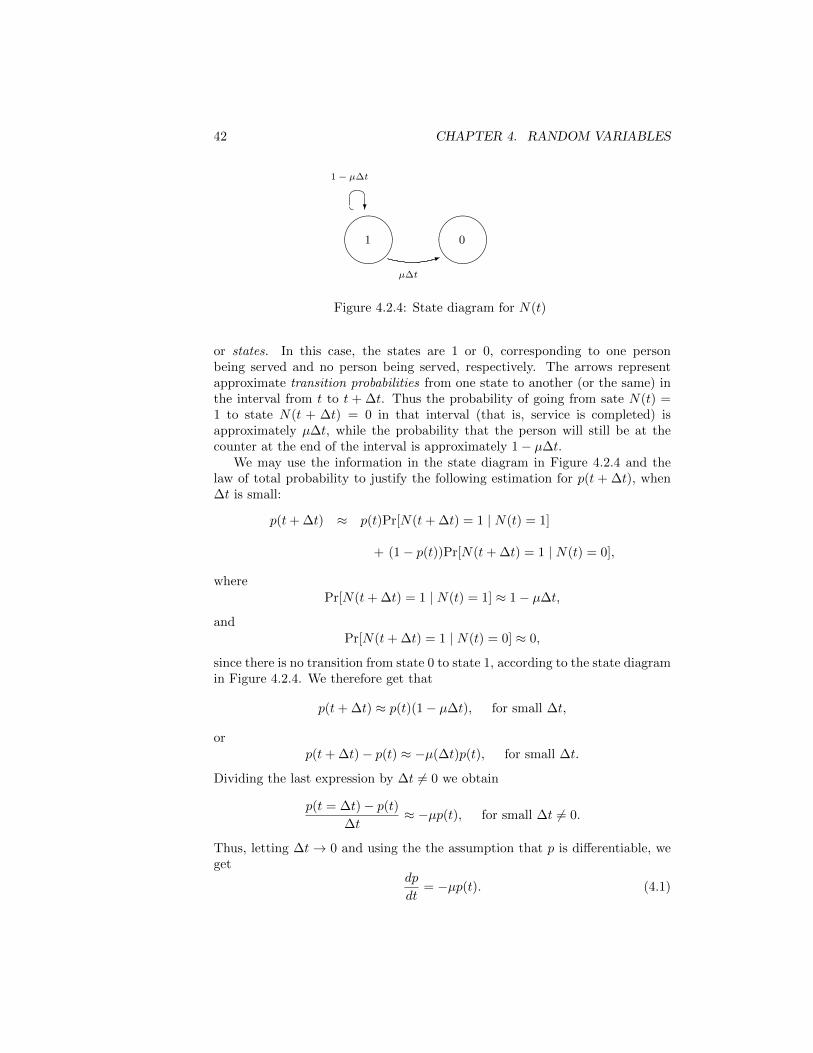
42 CHAPTER 4. RANDOM VARIABLES
"!# "!#
1− µ∆t
1 0
�� �?1
µ∆t
Figure 4.2.4: State diagram for N(t)
or states. In this case, the states are 1 or 0, corresponding to one personbeing served and no person being served, respectively. The arrows representapproximate transition probabilities from one state to another (or the same) inthe interval from t to t + ∆t. Thus the probability of going from sate N(t) =1 to state N(t + ∆t) = 0 in that interval (that is, service is completed) isapproximately µ∆t, while the probability that the person will still be at thecounter at the end of the interval is approximately 1− µ∆t.
We may use the information in the state diagram in Figure 4.2.4 and thelaw of total probability to justify the following estimation for p(t + ∆t), when∆t is small:
p(t+ ∆t) ≈ p(t)Pr[N(t+ ∆t) = 1 | N(t) = 1]
+ (1− p(t))Pr[N(t+ ∆t) = 1 | N(t) = 0],
wherePr[N(t+ ∆t) = 1 | N(t) = 1] ≈ 1− µ∆t,
andPr[N(t+ ∆t) = 1 | N(t) = 0] ≈ 0,
since there is no transition from state 0 to state 1, according to the state diagramin Figure 4.2.4. We therefore get that
p(t+ ∆t) ≈ p(t)(1− µ∆t), for small ∆t,
orp(t+ ∆t)− p(t) ≈ −µ(∆t)p(t), for small ∆t.
Dividing the last expression by ∆t 6= 0 we obtain
p(t = ∆t)− p(t)∆t
≈ −µp(t), for small ∆t 6= 0.
Thus, letting ∆t → 0 and using the the assumption that p is differentiable, weget
dp
dt= −µp(t). (4.1)
4.2. DISTRIBUTION FUNCTIONS 43
Notice that we no longer have and approximate result; this is possible by theassumption of differentiability of p(t).
Since p(0) = 1, it follows form (4.1) that p(t) = e−µt for t > 0.
Recall that T denotes the time it takes for service to be completed, or theservice time at the checkout counter. Thus, the event (T > t) is equivalent tothe event (N(t) = 1), since T > t implies that service has not been completedat time t and, therefore, N(t) = 1 at that time. It then follows that
Pr[T > t] = Pr[N(t) = 1]= p(t)= e−µt
for all t > 0; so that
Pr[T ≤ t] = 1− e−µt, for t > 0.
Thus, T is a continuous random variable with cdf
FT
(t) =
{1− e−µt, if t > 0;
0, elsewhere.(4.2)
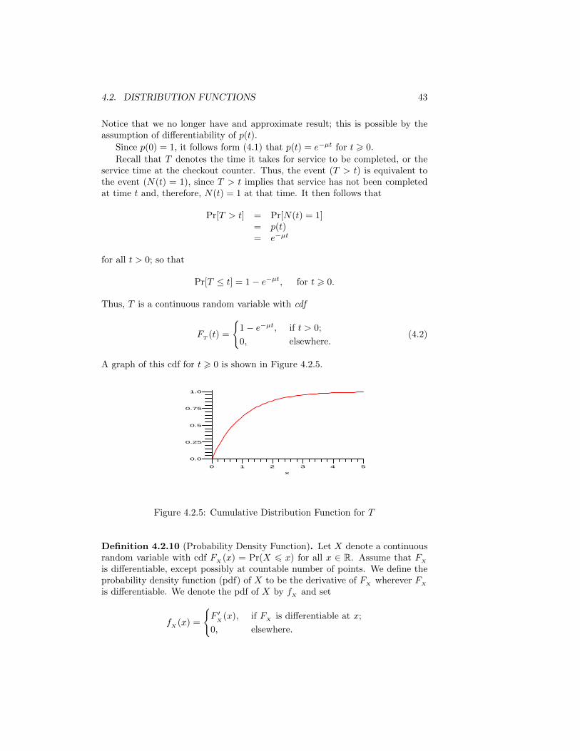
A graph of this cdf for t > 0 is shown in Figure 4.2.5.
0
0.75
x
54321
1.0
0.5
0.25
0.0
Figure 4.2.5: Cumulative Distribution Function for T
Definition 4.2.10 (Probability Density Function). Let X denote a continuousrandom variable with cdf F
X(x) = Pr(X 6 x) for all x ∈ R. Assume that F
X
is differentiable, except possibly at countable number of points. We define theprobability density function (pdf) of X to be the derivative of F
Xwherever F
X
is differentiable. We denote the pdf of X by fX
and set
fX
(x) =
{F ′X
(x), if FX
is differentiable at x;
0, elsewhere.

44 CHAPTER 4. RANDOM VARIABLES
Example 4.2.11. In the service time example, Example 4.2.9, if T is the timethat it takes for service to be completed at a checkout counter, then the cdf forT is as given in (4.2),
FT
(t) =
{1− e−µt, for t > 0;
0, elsewhere.
It then follows from Definition 4.2.10 that
fT
(t) =
{µe−µt, for t > 0;
0, elsewhere,
is the pdf for T , and we say that T follows an exponential distributionwith parameter 1/µ. We will see the significance of this parameter in the nextchapter.
In general, given a function f : R→ R, which is non–negative and integrablewith ∫ ∞
−∞f(x) dx = 1,
f defines the pdf for some continuous random variable X. In fact, the cdf forX is defined by
FX
(x) =
∫ x
−∞f(t) dt for all x ∈ R.
Example 4.2.12. Let a and b be real numbers with a < b. The function
f(x) =
1
b− aif a < x < b,
0 otherwise,
defines a pdf since ∫ ∞−∞
f(x) dx =
∫ b
a
1
b− adx = 1,
and f is non–negative.
Definition 4.2.13 (Uniform Distribution). A continuous random variable, X,having the pdf given in the previous example is said to be uniformly distributedon the interval (a, b). We write
X ∼ Uniform(a, b).
Example 4.2.14 (Finding the distribution for the square of a random variable).Let X ∼ Uniform(−1, 1) and Y = X2 give the pdf for Y .
4.2. DISTRIBUTION FUNCTIONS 45
Solution: Since X ∼ Uniform(−1, 1) its pdf is given by
fX
(x) =
1
2if − 1 < x < 1,
0 otherwise.
We would like to compute fY
(y) for 0 < y < 1. In order to do this, first wecompute the cdf F
Y(y) for 0 < y < 1:
FY
(y) = Pr(Y 6 y), for 0 < y < 1,= Pr(X2 6 y)= Pr(|Y | 6 √y)= Pr(−√y 6 X 6 √y)= Pr(−√y < X 6
√y), since X is continuous,
= Pr(X 6√y)− Pr(X 6 −√y)
= FX
(√y)− F
x(−√y).
Differentiating with respect to y we then obtain that
fY
(y) =d
dyFY
(y)
=d
dyFX
(√y)− d
dyFX
(−√y)
= F ′X
(√y) · d
dy
√y − F ′
X(−√y)
d
dy(−√y),
by the Chain Rule, so that
fY
(y) = fX
(√y) · 1
2√y
+ f ′X
(−√y)1
2√y
=1
2· 1
2√y
+1
2· 1
2√y
=1
2√y
for 0 < y < 1. We then have that
fY
(y) =
1
2√y, if 0 < y < 1;
0, otherwise.
�

46 CHAPTER 4. RANDOM VARIABLES
Chapter 5
Expectation of RandomVariables
5.1 Expected Value of a Random Variable
Definition 5.1.1 (Expected Value of a Continuous Random Variable). Let Xbe a continuous random variable with pdf f
X. If
∫ ∞−∞|x|f
X(x) dx <∞,
we define the expected value of X, denoted E(X), by
E(X) =
∫ ∞−∞
xfX
(x) dx.
Example 5.1.2 (Average Service Time). In the service time example, Example4.2.9, we showed that the time, T , that it takes for service to be completed atcheckout counter has an exponential distribution with pdf
fT
(t) =
{µe−µt, for t > 0;
0, otherwise,
where µ is a positive constant.
47

48 CHAPTER 5. EXPECTATION OF RANDOM VARIABLES
Observe that∫ ∞−∞|t|f
T(t) dt =
∫ ∞0
tµe−µt dt
= limb→∞
∫ b
0
t µe−µt dt
= limb→∞
[−te−µt − 1
µe−µt
]b0
= limb→∞
[1
µ− be−µb − 1
µe−µb
]
=1
µ,
where we have used integration by parts and L’Hospital’s rule. It then followsthat ∫ ∞
−∞|t|f
T(t) dt =
1
µ<∞
and therefore the expected value of T exists and
E(T ) =
∫ ∞−∞
tfT
(t) dt =
∫ ∞0
tµe−µt dt =1
µ.
Thus, the parameter µ is the reciprocal of the expected service time, or averageservice time, at the checkout counter.
Example 5.1.3. Suppose the average service time, or mean service time, ata checkout counter is 5 minutes. Compute the probability that a given personwill spend at least 6 minutes at the checkout counter.
Solution: We assume that the service time, T , is exponentially distributedwith pdf
fT
(t) =
{µe−µt, for t > 0;
0, otherwise,
where µ = 1/5. We then have that
Pr(T > 6) =
∫ ∞6
fT
(t) dt =
∫ ∞6
1
5e−t/5 dt = e−6/5 ≈ 0.30.
Thus, there is a 30% chance that a person will spend 6 minutes or more at thecheckout counter. �
Definition 5.1.4 (Exponential Distribution). A continuous random variable,X, is said to be exponentially distributed with parameter β > 0, written
X ∼ Exponential(β),
5.1. EXPECTED VALUE OF A RANDOM VARIABLE 49
if it has a pdf given by
fX
(x) =
1
βe−x/β for x > 0,
0 otherwise.
The expected value of X ∼ Exponential(β), for β > 0, is E(X) = β.
Example 5.1.5 (A Distribution without Expectation). Let X ∼ Uniform(0, 1)and define Y = 1/X. We determine the distribution for Y and show that Ydoes not have an expected value. In order to do this, we need to compute f
Y(y)
and then check that the integral∫ ∞−∞|y|f
Y(y) dy
does not converge.
To find fY
(y), we first determine the cdf of Y . Observe that possible valuesfor Y are y > 1, since possible values for X are 0 < x < 1.
FY
(y) = Pr(Y 6 y), for 1 < y <∞,= Pr(1/X 6 y)= Pr(X > 1/y)= Pr(X > 1/y), (since X is continuous),= 1− Pr(X 6 1/y)= 1− F
X(1/y).
Differentiating with respect to y we then obtain
fY
(y) =d
dyFY
(y), for 1 < y <∞,
=d
dy(1− F
X(1/y))
= −F ′X
(1/y)d
dy(1/y)
= fX
(1/y)1
y2.
We then have that
fY
(y) =
1
y2if 1 < y <∞
0 if y 6 1.
50 CHAPTER 5. EXPECTATION OF RANDOM VARIABLES
Next, compute ∫ ∞−∞|y|f
Y(y) dy =
∫ ∞1
|y| 1
y2dy
= limb→∞
∫ b
1
1
ydy
= limb→∞
ln b =∞.
Thus, ∫ ∞−∞|y|f
Y(y) dy =∞.
Consequently, Y = 1/X has no expectation.
Definition 5.1.6 (Expected Value of a Discrete Random Variable). Let X bea discrete random variable with pmf p
X. If∑
x
|x|pX
(x) <∞,
we define the expected value of X, denoted E(X), by
E(X) =∑x
x · pX
(x).
Thus, if X has a finite set of possible values, x1, x2, . . . , xn, and pmf pX
,then the expected value of X is
E(X) =
n∑k=1
xk · pX (xk).
On the other hand if X takes on a sequence of values, x1, x2, x3, . . . , then theexpected value of X exists provided that
∞∑k=1
|xk|pX (xk) <∞. (5.1)
If (5.1) holds true, then
E(X) =
∞∑k=1
xk · pX (xk).
Example 5.1.7. Let X denote the number on the top face of a balanced die.Compute E(X).
Solution: In this case the pmf of X is pX
(x) = 1/6 for x = 1, 2, 3, 4, 5, 6,zero elsewhere. Then,
E(X) =
6∑k=1
kpX
(k) =
6∑k=1
k · 1
6=
7
2= 3.5.
�
5.1. EXPECTED VALUE OF A RANDOM VARIABLE 51
Definition 5.1.8 (Bernoulli Trials). A Bernoulli Trial, X, is a discrete ran-dom variable that takes on only the values of 0 and 1. The event (X = 1) iscalled a “success”, while (X = 0) is called a “failure.” The probability of asuccess is denoted by p, where 0 < p < 1. We then have that the pmf of X is
pX
(x) =
1− p if x = 0,
p if x = 1,
0 elsewhere.
If a discrete random variable X has this pmf, we write
X ∼ Bernoulli(p),
and say that X is a Bernoulli trial with parameter p.
Example 5.1.9. Let X ∼ Bernoulli(p). Compute E(X).Solution: Compute E(X) = 0 · p
X(0) + 1 · p
X(1) = p, �
Example 5.1.10 (Expected Value of a Geometric Distribution). Imagine anexperiment consisting of performing a sequence of independent Bernoulli trialswith parameter p, with 0 < p < 1, until a 1 is obtained. Let X denote thenumber of trials until the first 1 is obtained. Then X is a discrete randomvariable with pmf
pX
(k) =
{(1− p)k−1p, for k = 1, 2, 3, . . . ;
0, elsewhere.(5.2)
To see how (5.2) comes about, note that X = k, fork > 1, if there are k − 1
zeros before the kth one, and the outcomes of the trials are independent. Thus,in order to show that X has an expected value, we need to check that
∞∑k=1
k(1− p)k−1p <∞. (5.3)
Observe thatd
dp[(1− p)k] = −k(1− p)k−1;
thus, the sum in (5.3) can be rewritten as
∞∑k=1
k(1− p)k−1p = −p∞∑k=1
d
dp[(1− p)k] (5.4)
Interchanging the differentiation and the summation in (5.4) we have that
∞∑k=1
k(1− p)k−1p = −p ddp
[ ∞∑k=1
(1− p)k]. (5.5)
52 CHAPTER 5. EXPECTATION OF RANDOM VARIABLES
Then, adding up the geometric series on the right–hand side of (5.5),
∞∑k=1
k(1− p)k−1p = −p ddp
[1− p
1− (1− p)
],
from which we get that
∞∑k=1
k(1− p)k−1p = −p ddp
[1
p− 1
]= −p ·
[− 1
p2
]=
1
p<∞.
We have therefore demonstrated that, if X ∼ Geometric(p), with 0 < p < 1,then E(X) exists and
E(X) =1
p.
Definition 5.1.11 (Independent Discrete Random Variable). Two discrete ran-dom variables X and Y are said to independent if and only if
Pr(X = x, Y = y) = Pr(X = x) · Pr(Y = y)
for all values, x, of X and all values, y, of Y .
Note: the event (X = x, Y = y) denotes the event (X = x) ∩ (Y = y); that is,the events (X = x) and (Y = y) occur jointly.
Example 5.1.12. Suppose X1 ∼ Bernoulli(p) and X2 ∼ Bernoulli(p) are inde-pendent random variables with 0 < p < 1. Define Y2 = X1 +X2. Find the pmffor Y2 and compute E(Y2).
Solution: Observe that Y2 takes on the values 0, 1 and 2. We compute
Pr(Y2 = 0) = Pr(X1 = 0, X2 = 0)= Pr(X1 = 0) · Pr(X2 = 0), by independence,= (1− p) · (1− p)= (1− p)2.
Next, since the event (Y2 = 1) consists of the disjoint union of the events(X1 = 1, X2 = 0) and (X1 = 0, X2 = 1),
Pr(Y2 = 1) = Pr(X1 = 1, X2 = 0) + Pr(X1 = 0, X2 = 1)= Pr(X1 = 1) · Pr(X2 = 0) + Pr(X1 = 0) · Pr(X2 = 1)= p(1− p) + (1− p)p= 2p(1− p).
Finally,Pr(Y2 = 2) = Pr(X1 = 1, X2 = 1)
= Pr(X1 = 1) · Pr(X2 = 1)= p · p= p2.
5.1. EXPECTED VALUE OF A RANDOM VARIABLE 53
We then have that the pmf of Y2 is given by
pY2
(y) =
(1− p)2 if y = 0,
2p(1− p) if y = 1,
p2 if y = 2,
0 elsewhere.
To find E(Y2), compute
E(Y2) = 0 · pY2
(0) + 1 · pY2
(1) + 2 · pY2
(2)= 2p(1− p) + 2p2
= 2p[(1− p) + p]= 2p.
�
We shall next consider the case in which we add three mutually independentBernoulli trials. Before we present this example, we give a precise definition ofmutual independence.
Definition 5.1.13 (Mutual Independent Discrete Random Variable). Threediscrete random variables X1, X2 and X3 are said to mutually independentif and only if
(i) they are pair–wise independent; that is,
Pr(Xi = xi, Xj = xj) = Pr(Xi = xi) · Pr(Xj = xj) for i 6= j,
for all values, xi, of Xi and all values, xj , of Xj ;
(ii) and
Pr(X1 = x1, X2 = x2, X3 = x3) = Pr(X1 = x1)·Pr(X2 = x2)·Pr(X3 = x3).
Lemma 5.1.14. Let X1, X2 and X3 be mutually independent, discrete randomvariables and define Y2 = X1 +X2. Then, Y2 and X3 are independent.
Proof: Compute
Pr(Y2 = w,X3 = z) = Pr(X1 +X2 = w,X3 = z)
=∑x
Pr(X1 = x,X2 = w − x,X3 = z),
where the summation is taken over possible value of X1. It then follows that
Pr(Y2 = w,X3 = z) =∑x
Pr(X1 = x) · Pr(X2 = w − x) · Pr(X3 = z),
54 CHAPTER 5. EXPECTATION OF RANDOM VARIABLES
where we have used (ii) in Definition 5.1.13. Thus, by pairwise independence,(i.e., (i) in Definition 5.1.13),
Pr(Y2 = w,X3 = z) =
(∑x
Pr(X1 = x) · Pr(X2 = w − x)
)· Pr(X3 = z)
= Pr(X1 +X2 = w) · Pr(X3 = z)
= Pr(Y2 = w) · Pr(X3 = z),
which shows the independence of Y2 and X3.
Example 5.1.15. Suppose X1, X2 and X3 be three mutually independentBernoulli random variables with parameter p, where 0 < p < 1. Define Y3 =X1 +X2 +X3. Find the pmf for Y3 and compute E(Y3).
Solution: Observe that Y3 takes on the values 0, 1, 2 and 3, and that
Y3 = Y2 +X3,
where the pmf and expected value of Y2 were computed in Example 5.1.12.We compute
Pr(Y3 = 0) = Pr(Y2 = 0, X3 = 0)= Pr(Y2 = 0) · Pr(X3 = 0), by independence (Lemma 5.1.14),= (1− p)2 · (1− p)= (1− p)3.
Next, since the event (Y3 = 1) consists of the disjoint union of the events(Y2 = 1, X3 = 0) and (Y2 = 0, X3 = 1),
Pr(Y3 = 1) = Pr(Y2 = 1, X3 = 0) + Pr(Y2 = 0, X3 = 1)= Pr(Y2 = 1) · Pr(X3 = 0) + Pr(Y2 = 0) · Pr(X3 = 1)= 2p(1− p)(1− p) + (1− p)2p= 3p(1− p)2.
Similarly,
Pr(Y3 = 2) = Pr(Y2 = 2, X3 = 0) + Pr(Y2 = 1, X3 = 1)= Pr(Y2 = 2) · Pr(X3 = 0) + Pr(Y2 = 1) · Pr(X3 = 1)= p2(1− p) + 2p(1− p)p= 3p2(1− p),
andPr(Y3 = 3) = Pr(Y2 = 2, X3 = 1)
= Pr(Y2 = 0) · Pr(X3 = 0)= p2 · p= p3.
5.1. EXPECTED VALUE OF A RANDOM VARIABLE 55
We then have that the pmf of Y3 is
pY3
(y) =
(1− p)3 if y = 0,
3p(1− p)2 if y = 1,
3p2(1− p) if y = 2,
p3 if y = 3,
0 elsewhere.
To find E(Y2), compute
E(Y3) = 0 · pY3
(0) + 1 · pY3
(1) + 2 · pY3
(2) + 3 · pY3
(3)= 3p(1− p)2 + 2 · 3p2(1− p) + 3p3
= 3p[(1− p)2 + 2p(1− p) + p2]= 3p[(1− p) + p]2
= 3p.
�
If we go through the calculations in Examples 5.1.12 and 5.1.15 for the case offour mutually independent1 Bernoulli trials with parameter p, where 0 < p < 1,X1, X2, X3 and X4, we obtain that for Y4 = X1 +X2 +X3 +X4,
pY4
(y) =
(1− p)4 if y = 0,
4p(1− p)3 if y = 1,
6p2(1− p)2 if y = 2
4p3(1− p) if y = 3
p4 if y = 4,
0 elsewhere,
and
E(Y4) = 4p.
Observe that the terms in the expressions for pY2
(y), pY3
(y) and pY4
(y) are theterms in the expansion of [(1− p) + p]n for n = 2, 3 and 4, respectively. By theBinomial Expansion Theorem,
[(1− p) + p]n =
n∑k=0
(n
k
)pk(1− p)n−k,
where (n
k
)=
n!
k!(n− k)!, k = 0, 1, 2 . . . , n,
1Here, not only do we require that the random variable be pairwise independent, but alsothat for any group of k ≥ 2 events (Xj = xj), the probability of their intersection is theproduct of their probabilities.

56 CHAPTER 5. EXPECTATION OF RANDOM VARIABLES
are the called the binomial coefficients. This suggests that if
Yn = X1 +X2 + · · ·+Xn,
where X1, X2, . . . , Xn are n mutually independent Bernoulli trials with param-eter p, for 0 < p < 1, then
pYn
(k) =
(n
k
)pk(1− p)n−k for k = 0, 1, 2, . . . , n.
Furthermore,
E(Yn) = np.
We shall establish this as a the following Theorem:
Theorem 5.1.16. Assume that X1, X2, . . . , Xn are mutually independent Bernoullitrials with parameter p, with 0 < p < 1. Define
Yn = X1 +X2 + · · ·+Xn.
Then the pmf of Yn is
pYn
(k) =
(n
k
)pk(1− p)n−k for k = 0, 1, 2, . . . , n,
and
E(Yn) = np.
Proof: We prove this result by induction on n. For n = 1 we have that Y1 = X1,and therefore
pY1
(0) = Pr(X1 = 0) = 1− p
and
pY1
(1) = Pr(X1 = 1) = p.
Thus,
pY1
(k) =
1− p if k = 0,
p if k = 1,
0 elsewhere.
Observe that
(1
0
)=
(1
1
)= 1 and therefore the result holds true for n = 1.
Next, assume the theorem is true for n; that is, suppose that
pYn
(k) =
(n
k
)pk(1− p)n−k for k = 0, 1, 2, . . . , n, (5.6)
and that
E(Yn) = np. (5.7)
5.1. EXPECTED VALUE OF A RANDOM VARIABLE 57
We need to show that the result also holds true for n + 1. In other words,we show that if X1, X2, . . . , Xn, Xn+1 are mutually independent Bernoulli trialswith parameter p, with 0 < p < 1, and
Yn+1 = X1 +X2 + · · ·+Xn +Xn+1, (5.8)
then, the pmf of Yn+1 is
pYn+1
(k) =
(n+ 1
k
)pk(1− p)n+1−k for k = 0, 1, 2, . . . , n, n+ 1, (5.9)
andE(Yn+1) = (n+ 1)p. (5.10)
From (5.10) we see that
Yn+1 = Yn +Xn+1,
where Yn and Xn+1 are independent random variables, by an argument similarto the one in the proof of Lemma 5.1.14 since the Xk’s are mutually independent.Therefore, the following calculations are justified:
(i) for k 6 n,
Pr(Yn+1 = k) = Pr(Yn = k,Xn+1 = 0) + Pr(Yn = k − 1, Xn+1 = 1)
= Pr(Yn = k) · Pr(Xn+1 = 0)+Pr(Yn = k − 1) · Pr(Xn−1 = 1)
=
(n
k
)pk(1− p)n−k(1− p)
+
(n
k − 1
)pk−1(1− p)n−k+1p,
where we have used the inductive hypothesis (5.6). Thus,
Pr(Yn+1 = k) =
[(n
k
)+
(n
k − 1
)]pk(1− p)n+1−k.
The expression in (5.9) will following from the fact that(n
k
)+
(n
k − 1
)=
(n+ 1
k
),
which can be established by the following counting argument:
Imagine n + 1 balls in a bag, n of which are blue and one isred. We consider the collection of all groups of k balls that canbe formed out of the n + 1 balls in the bag. This collection is
58 CHAPTER 5. EXPECTATION OF RANDOM VARIABLES
made up of two disjoint sub–collections: the ones with the redball and the ones without the red ball. The number of elementsin the collection with the one red ball is(
n
k − 1
)·(
1
1
)=
(n
k − 1
),
while the number of elements in the collection of groups withoutthe red ball are (
n
k
).
Adding these two must yield
(n+ 1
k
).
(ii) If k = n+ 1, then
Pr(Yn+1 = k) = Pr(Yn = n,Xn+1 = 1)= Pr(Yn = n) · Pr(Xn+1 = 1)= pnp= pn+1
=
(n+ 1
k
)pk(1− p)n+1−k,
since k = n+ 1.
Finally, to establish (5.10) based on (5.7), use the result of Problem 2 inAssignment 10 to show that, since Yn and Xn are independent,
E(Yn+1) = E(Yn +Xn+1) = E(Yn) + E(Xn+1) = np+ p = (n+ 1)p.
Definition 5.1.17 (Binomial Distribution). Let n be a natural number and0 < p < 1. A discrete random variable, X, having pmf
pX
(k) =
(n
k
)pk(1− p)n−k for k = 0, 1, 2, . . . , n,
is said to have a binomial distribution with parameters n and p.We write X ∼ Binomial(n, p).
Remark 5.1.18. In Theorem 5.1.16 we showed that if X ∼ Binomial(n, p),then
E(X) = np.
We also showed in that theorem that the sum of n mutually independentBernoulli trials with parameter p, for 0 < p < 1, follows a Binomial distri-bution with parameters n and p.
5.2. PROPERTIES OF EXPECTATIONS 59
Definition 5.1.19 (Independent Identically Distributed Random Variables). Aset of random variables, {X1, X2, . . . , Xn}, is said be independent identicallydistributed, or iid, if the random variables are mutually disjoint and if theyall have the same distribution function.
If the random variables X1, X2, . . . , Xn are iid, then they form a simplerandom sample of size n.
Example 5.1.20. LetX1, X2, . . . , Xn be a simple random sample from a Bernoulli(p)distribution, with 0 < p < 1. Define the sample mean X by
X =X1 +X2 + · · ·+Xn
n.
Give the distribution function for X and compute E(X).Solution: Write Y = nX = X1 +X2 +· · ·+Xn. Then, since X1, X2, . . . , Xn
are iid Bernoulli(p) random variables, Theorem 5.1.16 implies that Y ∼ Binomial(n, p).Consequently, the pmf of Y is
pY
(k) =
(n
k
)pk(1− p)n−k for k = 0, 1, 2, . . . , n,
and E(Y ) = np.
Now, X may take on the values 0,1
n,
2
n, . . .
n− 1
n, 1, and
Pr(X = x) = Pr(Y = nx) for x = 0,1
n,
2
n, . . .
n− 1
n, 1,
so that
Pr(X = x) =
(n
nx
)pnx(1− p)n−nx for x = 0,
1
n,
2
n, . . .
n− 1
n, 1.
The expected value of X can be computed as follows
E(X) = E
(1
nY
)=
1
nE(Y ) =
1
n(np) = p.
Observe that X is the proportion of successes in the simple random sample. Itthen follows that the expected proportion of successes in the random sample isp, the probability of a success. �
5.2 Properties of Expectations
5.2.1 Linearity
We have already mentioned (and used) the fact that
E(X + Y ) = E(X) + E(Y ), (5.11)
60 CHAPTER 5. EXPECTATION OF RANDOM VARIABLES
for the case of independent, discrete random variable X and Y (see Problem 6in Assignment #5). The expression in (5.11) is true in general, regardless ofwhether or not X are discrete or independent. This will be shown to be thecase in the context of joint distributions in a subsequent section.
We can also verify, using the definition of expected value (see Definition 5.1.1and ) that, for any constant c,
E(cX) = cE(X). (5.12)
The expressions in (5.11) and (5.12) say that expectation is a linear operation.
5.2.2 Expectations of Functions of Random Variables
Example 5.2.1. Let X denote a continuous random variable with pdf
fX
(x) =
{3x2 if 0 < x < 1,
0 otherwise.
Compute the expected value of X2.We show two ways to compute E(X).
(i) First Alternative. Let Y = X2 and compute the pdf of Y . To do this, firstwe compute the cdf:
FY
(y) = Pr(Y 6 y), for 0 < y < 1,= Pr(X2 6 y)= Pr(|X| 6 √y)= Pr(−√y 6 |X| 6 √y)= Pr(−√y < |X| 6 √y), since X is continuous,= F
X(√y)− F
X(−√y)
= FX
(√y),
since fX
is 0 for negative values.
It then follows that
fY
(y) = F ′X
(√y) · d
dy(√y)
= fX
(√y) · 1
2√y
= 3(√y)2 · 1
2√y
=3
2
√y
for 0 < y < 1.
5.2. PROPERTIES OF EXPECTATIONS 61
Consequently, the pdf for Y is
fY
(y) =
3
2
√y if 0 < y < 1,
0 otherwise.
Therefore,E(X2) = E(Y )
=
∫ ∞−∞
yfY
(y) dy
=
∫ 1
0
y3
2
√y dy
=3
2
∫ 1
0
y3/2 dy
=3
2· 2
5
=3
5.
(ii) Second Alternative. Alternatively, we could have compute E(X2) by eval-uating ∫ ∞
−∞x2f
X(x) dx =
∫ 1
0
x2 · 3x2 dx
=3
5.
The fact that both ways of evaluating E(X2) presented in the previousexample is a consequence of the following general result.
Theorem 5.2.2. Let X be a continuous random variable and g denote a con-tinuous function defined on the range of X. Then, if∫ ∞
−∞|g(x)|f
X(x) dx <∞,
E(g(X)) =
∫ ∞−∞
g(x)fX
(x) dx.
Proof: We prove this result for the special case in which g is differentiable withg′(x) > 0 for all x in the range of X. In this case g is strictly increasing andit therefore has an inverse function g−1 mapping onto the range of g ◦ X andwhich is also differentiable with derivative given by
d
dy
[g−1(y)
]=
1
g′(x)=
1
g′(g−1(y)),
62 CHAPTER 5. EXPECTATION OF RANDOM VARIABLES
where we have set y = g(x) for all x in the range of X, or Y = g(X). Assumealso that the values of X range from −∞ to ∞ and those of Y also range from−∞ to ∞. Thus, using the Change of Variables Theorem, we have that∫ ∞
−∞g(x)f
X(x) dx =
∫ ∞−∞
yfX
(g−1(y)) · 1
g′(g−1(y))dy,
since x = g−1(y) and therefore
dx =d
dy
[g−1(y)
]dy =
1
g′(g−1(y))dy.
On the other hand,FY
(y) = Pr(Y 6 y)= Pr(g(X) 6 y)= Pr(X 6 g−1(y))= F
X(g−1(y)),
from which we obtain, by the Chain Rule, that
fY
(y) = fX
(g−1(y)1
g′(g−1(y)).
Consequently, ∫ ∞−∞
yfY
(y) dy =
∫ ∞−∞
g(x)fX
(x) dx,
or
E(Y ) =
∫ ∞−∞
g(x)fX
(x) dx.
Theorem 5.2.2 also applies to functions of a discrete random variable. Inthis case we have
Theorem 5.2.3. Let X be a discrete random variable with pmf pX
, and let gdenote a function defined on the range of X. Then, if∑
x
|g(x)|pX
(x) <∞,
E(g(X)) =∑x
g(x)pX
(x).
5.3 Moments
Theorems 5.2.2 and 5.2.3 can be used to evaluate the expected values of powersof a random variable
E(Xm) =
∫ ∞−∞
xmfX
(x) dx, m = 0, 1, 2, 3, . . . ,

5.3. MOMENTS 63
in the continuous case, provided that∫ ∞−∞|x|mf
X(x) dx <∞, m = 0, 1, 2, 3, . . . .
In the discrete case we have
E(Xm) =∑x
xmpX
(x), m = 0, 1, 2, 3, . . . ,
provided that ∑x
|x|mpX
(x) <∞, m = 0, 1, 2, 3, . . . .
Definition 5.3.1 (mth Moment of a Distribution). E(Xm), if it exists, is calledthe mth moment of X for m = 0, 2, 3, . . .
Observe that the first moment of X is its expectation.
Example 5.3.2. Let X have a uniform distribution over the interval (a, b) fora < b. Compute the second moment of X.
Solution: Using Theorem 5.2.2 we get
E(X2) =
∫ ∞−∞
x2fX
(x) dx,
where
fX
(x) =
1
b− aif a < x < b,
0 otherwise.
Thus,
E(X2) =
∫ b
a
x2
b− adx
=
[1
b− ax3
3
]ba
=1
3(b− a)· (b3 − a3)
=b2 + ab+ a2
3.
�
5.3.1 Moment Generating Function
Using Theorems 5.2.2 or 5.2.3 we can also evaluate E(etX) whenever this ex-pectation is defined.
64 CHAPTER 5. EXPECTATION OF RANDOM VARIABLES
Example 5.3.3. Let X have an exponential distribution with parameter β > 0.Determine the values of t ∈ R for which E(etX) is defined and compute it.
Solution: The pdf of X is given by
fX
(x) =
1
βe−x/β if x > 0,
0 if x 6 0.
Then,
E(etX) =
∫ ∞−∞
etxfX
(x) dx
=1
β
∫ ∞0
etxe−x/β dx
=1
β
∫ ∞0
e−[(1/β)−t]x dx.
We note that for the integral in the last equation to converge, we must requirethat
t < 1/β.
For these values of t we get that
E(etX) =1
β· 1
(1/β)− t
=1
1− βt.
�
Definition 5.3.4 (Moment Generating Function). Given a random variable X,the expectation E(etX), for those values of t for which it is defined, is called themoment generating function, or mgf, of X, and is denoted by ψ
X(t). We
then have that
ψX
(t) = E(etX),
whenever the expectation is defined.
Example 5.3.5. If X ∼ Exponential(β), for β > 0, then Example 5.3.3 showsthat the mgf of X is given by
ψX
(t) =1
1− βtfor t <
1
β.
Example 5.3.6. Let X ∼ Binomial(n, p), for n > 1 and 0 < p < 1. Computethe mgf of X.

5.3. MOMENTS 65
Solution: The pmf of X is
pX
(k) =
(n
k
)pk(1− p)n−k for k = 0, 1, 2, . . . , n,
and therefore, by the law of the unconscious statistician,
ψX
(t) = E(etX)
=
n∑k=1
etkpX
(k)
=
n∑k=1
(et)k(n
k
)pk(1− p)n−k
=
n∑k=1
(n
k
)(pet)k(1− p)n−k
= (pet + 1− p)n,
where we have used the Binomial Theorem.We therefore have that if X is binomially distributed with parameters n and
p, then its mgf is given by
ψX
(t) = (1− p+ pet)n for all t ∈ R.
�
5.3.2 Properties of Moment Generating Functions
First observe that for any random variable X,
ψX
(0) = E(e0·X) = E(1) = 1.
The importance of the moment generating function stems from the fact that,if ψ
X(t) is defined over some interval around t = 0, then it is infinitely differ-
entiable in that interval and its derivatives at t = 0 yield the moments of X.More precisely, in the continuous cases, the m–the order derivative of ψ
Xat t
is given by
ψ(m)(t) =
∫ ∞−∞
xmetxfX
(x) dx, for all m = 0, 1, 2, 3, . . . ,
and all t in the interval around 0 where these derivatives are defined. It thenfollows that
ψ(m)(0) =
∫ ∞−∞
xmfX
(x) dx = E(Xm), for all m = 0, 1, 2, 3, . . . .

66 CHAPTER 5. EXPECTATION OF RANDOM VARIABLES
Example 5.3.7. Let X ∼ Exponential(β). Compute the second moment of X.Solution: From Example 5.3.5 we have that
ψX
(t) =1
1− βtfor t <
1
β.
Differentiating with respect to t we obtain
ψ′X
(t) =β
(1− βt)2for t <
1
β
and
ψ′′X
(t) =2β2
(1− βt)3for t <
1
β.
It then follows that E(X2) = ψ′′X
(0) = 2β2. �
Example 5.3.8. Let X ∼ Binomial(n, p). Compute the second moment of X.Solution: From Example 5.3.6 we have that
ψX
(t) = (1− p+ pet)n for all t ∈ R.
Differentiating with respect to t we obtain
ψ′X
(t) = npet(1− p+ pet)n−1
and
ψ′′X
(t) = npet(1− p+ pet)n−1 + npet(n− 1)pet(1− p+ pet)n−2
= npet(1− p+ pet)n−1 + n(n− 1)p2e2t(1− p+ pet)n−2
It then follows that E(X2) = ψ′′X
(0) = np+ n(n− 1)p2. �
A very important property of moment generating functions is the fact thatψX
, if it exists in some open interval around 0, completely determines the distri-bution of the random variable X. This fact is known as the Uniqueness Theoremfor Moment Generating Functions.
Theorem 5.3.9 (Uniqueness of Moment Generating Functions). Let X andY denote two random variables with moment generating functions ψ
Xand ψ
Y,
respectively. Suppose that there exists δ > 0 such ψX
(t) = ψY
(t) for −δ < t < δ.Then, X and Y have the same cumulative distribution functions; that is,
FX
(x) = FY
(x), for all x ∈ R.
A proof of this result may be found in an article by J. H. Curtiss in TheAnnals of Mathematical Statistics, Vol. 13, No. 4, (Dec., 1942), pp. 430-433.
We present an example of an application of Theorem 5.3.9
Example 5.3.10. Suppose that X is a random variable with mgf
ψX
(t) =1
1− 2t, for t <
1
2. (5.13)
Compute Pr(X > 2).
5.3. MOMENTS 67
Solution: Since the function in (5.13) gives the mgf of an Exponential(2)distribution, by the Uniqueness of Moment Generating Functions X must havean exponential distribution with parameter 2; so that
FX
(x) =
{1− e−x/2, for x > 0;
0, for x 6 0.
Thus, Pr(X > 2) = 1− FX
(2) = e−1. �
Example 5.3.11. Let x1, x2, . . . , xn denote real values. Let p1, p2, . . . , pn de-note positive values satisfying
n∑k=1
pk = 1.
Then, the function ψX
: R→ R given by
ψX
(t) = p1ex1t + p2e
x2t + · · ·+ pnexnt, for t ∈ R,
defines the mgf of a discrete random variable, X, with pmf
pX
(x) =
{pk, if x = xk, for k = 1, 2, . . . , n;
0, elsewhere.
Example 5.3.12. Let β be a positive parameter and a ∈ R. Find the distri-bution of a random variable, Y , with mgf
ψY
(t) =eat
1− βt, for t <
1
β. (5.14)
Solution: By the result in Example 5.3.5, if X ∼ Exponential(β), the Xhas mgf
ψX
(t) =1
1− βt, for t <
1
β. (5.15)
Consider the random variable Z = X + a and compute
ψZ
(t) = E(etZ),
to getψZ
(t) = E(et(X+a))
= E(etX+at)
= E(eatetX);
so that, using the linearity of the expectation,
ψZ
(t) = eatE(etX),
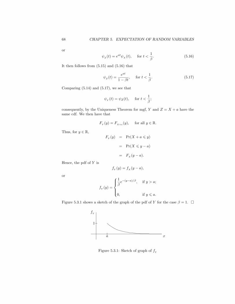
68 CHAPTER 5. EXPECTATION OF RANDOM VARIABLES
or
ψZ
(t) = eatψX
(t), for t <1
β. (5.16)
It then follows from (5.15) and (5.16) that
ψZ
(t) =eat
1− βt, for t <
1
β. (5.17)
Comparing (5.14) and (5.17), we see that
ψY
(t) = ψZ(t), for t <1
β;
consequently, by the Uniqueness Theorem for mgf, Y and Z = X + a have thesame cdf. We then have that
FY
(y) = FX+a
(y), for all y ∈ R.
Thus, for y ∈ R,
FY
(y) = Pr(X + a 6 y)
= Pr(X 6 y − a)
= FX
(y − a).
Hence, the pdf of Y is
fY
(y) = fX
(y − a),
or
fY
(y) =
1
βe−(y−a)/β , if y > a;
0, if y 6 a.
Figure 5.3.1 shows a sketch of the graph of the pdf of Y for the case β = 1. �
x
fY
1
a
Figure 5.3.1: Sketch of graph of fY
5.4. VARIANCE 69
5.4 Variance
Given a random variable X for which an expectation exists, define
µ = E(X).
µ is usually referred to as the mean of the random variable X. For givenm = 1, 2, 3, . . ., if E(|X − µ|m) <∞,
E[(X − µ)m]
is called the mth central moment of X. The second central moment of X,
E[(X − µ)2],
if it exists, is called the variance of X and is denoted by Var(X). We thenhave that
Var(X) = E[(X − µ)2],
provided that the expectation and second moment of X exist. The variance ofX measures the average square deviation of the distribution of X from itsmean. Thus, √
E[(X − µ)2]
is a measure of deviation from the mean. It is usually denoted by σ and is calledthe standard deviation form the mean. We then have
Var(X) = σ2.
We can compute the variance of a random variable X as follows:
Var(X) = E[(X − µ)2]= E(X2 − 2µX + µ2)= E(X2)− 2µE(X) + µ2E(1))= E(X2)− 2µ · µ+ µ2
= E(X2)− µ2.
Example 5.4.1. Let X ∼ Exponential(β). Compute the variance of X.Solution: In this case µ = E(X) = β and, from Example 5.3.7, E(X2) =
2β2. Consequently,
Var(X) = E(X2)− µ2 = 2β2 − β2 = β2.
�
Example 5.4.2. Let X ∼ Binomial(n, p). Compute the variance of X.Solution: Here, µ = np and, from Example 5.3.8,
E(X2) = np+ n(n− 1)p2.
Thus,
Var(X) = E(X2)− µ2 = np+ n(n− 1)p2 − n2p2 = np(1− p).
�

70 CHAPTER 5. EXPECTATION OF RANDOM VARIABLES
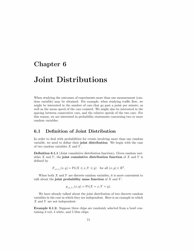
Chapter 6
Joint Distributions
When studying the outcomes of experiments more than one measurement (ran-dom variable) may be obtained. For example, when studying traffic flow, wemight be interested in the number of cars that go past a point per minute, aswell as the mean speed of the cars counted. We might also be interested in thespacing between consecutive cars, and the relative speeds of the two cars. Forthis reason, we are interested in probability statements concerning two or morerandom variables.
6.1 Definition of Joint Distribution
In order to deal with probabilities for events involving more than one randomvariable, we need to define their joint distribution. We begin with the caseof two random variables X and Y .
Definition 6.1.1 (Joint cumulative distribution function). Given random vari-ables X and Y , the joint cumulative distribution function of X and Y isdefined by
F(X,Y )
(x, y) = Pr(X 6 x, Y 6 y) for all (x, y) ∈ R2.
When both X and Y are discrete random variables, it is more convenient totalk about the joint probability mass function of X and Y :
p(X,Y )
(x, y) = Pr(X = x, Y = y).
We have already talked about the joint distribution of two discrete randomvariables in the case in which they are independent. Here is an example in whichX and Y are not independent:
Example 6.1.2. Suppose three chips are randomly selected from a bowl con-taining 3 red, 4 white, and 5 blue chips.
71
72 CHAPTER 6. JOINT DISTRIBUTIONS
Let X denote the number of red chips chosen, and Y be the number of whitechips chosen. We would like to compute the joint probability function of X andY ; that is,
Pr(X = x, Y = y),
were x and y range over 0, 1, 2 and 3.For instance,
Pr(X = 0, Y = 0) =
(53
)(123
) =10
220=
1
22,
Pr(X = 0, Y = 1) =
(41
)·(
52
)(123
) =40
220=
2
11,
Pr(X = 1, Y = 1) =
(31
)·(
41
)·(
51
)(123
) =60
220=
3
11,
and so on for all 16 of the joint probabilities. These probabilities are more easilyexpressed in tabular form:
X\Y 0 1 2 3 Row Sums0 1/22 2/11 3/22 2/110 21/551 3/22 3/11 9/110 0 27/552 3/42 3/55 0 0 27/2203 1/220 0 0 0 1/220
Column Sums 14/55 28/55 12/55 1/55 1
Table 6.1: Joint Probability Distribution for X and Y , p(X,Y )
Notice that pmf’s for the individual random variables X and Y can beobtained as follows:
pX
(i) =
3∑j=0
P (i, j)← adding up ith row
for i = 1, 2, 3, and
pY
(j) =
3∑i=0
P (i, j)← adding up jth column
for j = 1, 2, 3.These are expressed in Table 6.1 as “row sums” and “column sums,” respec-
tively, on the “margins” of the table. For this reason pX
and pY
are usuallycalled marginal distributions.
Observe that, for instance,
0 = Pr(X = 3, Y = 1) 6= pX
(3) · pY
(1) =1
220· 28
55,
and therefore X and Y are not independent.
6.1. DEFINITION OF JOINT DISTRIBUTION 73
Definition 6.1.3 (Joint Probability Density Function). An integrable functionf : R2 → R is said to be a joint pdf of the continuous random variables X andY iff
(i) f(x, y) > 0 for all (x, y) ∈ R2, and
(ii)
∫ ∞−∞
∫ ∞−∞
f(x, y) dxdy = 1.
Example 6.1.4. Consider the disk of radius 1 centered at the origin,
D1 = {(x, y) ∈ R2 | x2 + y2 < 1}.
The uniform joint distribution for the disc is given by the function
f(x, y) =
1
πif x2 + y2 < 1,
0 otherwise.
This is the joint pdf for two random variables, X and Y , since∫ ∞−∞
∫ ∞−∞
f(x, y) dxdy =
∫∫D1
1
πdxdy =
1
π· area(D1) = 1,
since area(D1) = π.This pdf models a situation in which the random variables X and Y denote
the coordinates of a point on the unit disk chosen at random.
If X and Y are continuous random variables with joint pdf f(X,Y )
, then thejoint cumulative distribution function, F
(X,Y ), is given by
F(X,Y )
(x, y) = Pr(X ≤ x, Y ≤ y) =
∫ x
−∞
∫ y
−∞f
(X,Y )(u, v) dvdu,
for all (x, y) ∈ R2.Given the joint pdf, f
(X,Y ), of two random variables defined on the same
sample space, C, we can compute the probability of events of the form
((X,Y ) ∈ A) = {c ∈ C | (X(c), Y (c)) ∈ A},
where A is a Borel subset1 of R2, is computed as follows
Pr((X,Y ) ∈ A) =
∫∫A
f(X,Y )
(x, y) dxdy.
1Borel sets in R2 are generated by bounded open disks; i.e, the sets
{(x, y) ∈ R2 | (x− xo)2 + (y − yo)
2 < r2},
where (xo, yo) ∈ R2 and r > 0.
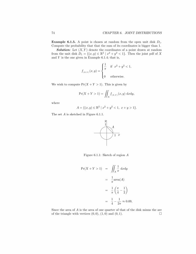
74 CHAPTER 6. JOINT DISTRIBUTIONS
Example 6.1.5. A point is chosen at random from the open unit disk D1.Compute the probability that that the sum of its coordinates is bigger than 1.
Solution: Let (X,Y ) denote the coordinates of a point drawn at randomfrom the unit disk D1 = {(x, y) ∈ R2 | x2 + y2 < 1}. Then the joint pdf of Xand Y is the one given in Example 6.1.4; that is,
f(X,Y )
(x, y) =
1
πif x2 + y2 < 1,
0 otherwise.
We wish to compute Pr(X + Y > 1). This is given by
Pr(X + Y > 1) =
∫∫A
f(X,Y )
(x, y) dxdy,
where
A = {(x, y) ∈ R2 | x2 + y2 < 1, x+ y > 1}.
The set A is sketched in Figure 6.1.1.
x
y
@@
1
1
&%'$A
Figure 6.1.1: Sketch of region A
Pr(X + Y > 1) =
∫∫A
1
πdxdy
=1
πarea(A)
=1
π
(π
4− 1
2
)
=1
4− 1
2π≈ 0.09,
Since the area of A is the area of one quarter of that of the disk minus the areof the triangle with vertices (0, 0), (1, 0) and (0, 1). �
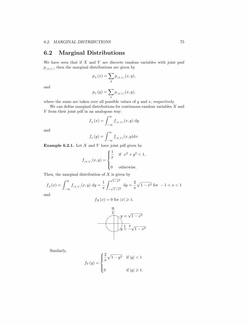
6.2. MARGINAL DISTRIBUTIONS 75
6.2 Marginal Distributions
We have seen that if X and Y are discrete random variables with joint pmfp
(X,Y ), then the marginal distributions are given by
pX
(x) =∑y
p(X,Y )
(x, y),
andpY
(y) =∑x
p(X,Y )
(x, y),
where the sums are taken over all possible values of y and x, respectively.We can define marginal distributions for continuous random variables X and
Y from their joint pdf in an analogous way:
fX
(x) =
∫ ∞−∞
f(X,Y )
(x, y) dy
and
fY
(y) =
∫ ∞−∞
f(X,Y )
(x, y)dx.
Example 6.2.1. Let X and Y have joint pdf given by
f(X,Y )
(x, y) =
1
πif x2 + y2 < 1,
0 otherwise.
Then, the marginal distribution of X is given by
fX
(x) =
∫ ∞−∞
f(X,Y )
(x, y) dy =1
π
∫ √1−x2
−√
1−x2
dy =2
π
√1− x2 for − 1 < x < 1
andfX(x) = 0 for |x| > 1.
x
y
1
1
&%'$y =
√1− x2
y = −√
1− x2
Similarly,
fY (y) =
2
π
√1− y2 if |y| < 1
0 if |y| > 1.
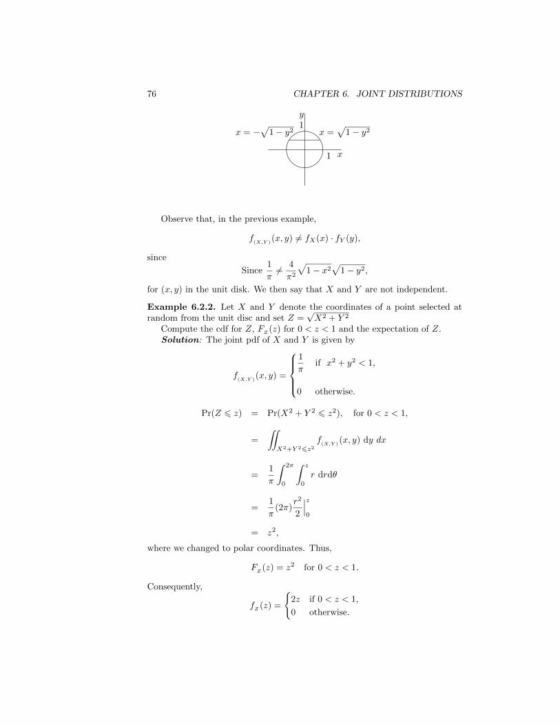
76 CHAPTER 6. JOINT DISTRIBUTIONS
x
y
1
1
&%'$x =
√1− y2x = −
√1− y2
Observe that, in the previous example,
f(X,Y )
(x, y) 6= fX(x) · fY (y),
since
Since1
π6= 4
π2
√1− x2
√1− y2,
for (x, y) in the unit disk. We then say that X and Y are not independent.
Example 6.2.2. Let X and Y denote the coordinates of a point selected atrandom from the unit disc and set Z =
√X2 + Y 2
Compute the cdf for Z, FZ
(z) for 0 < z < 1 and the expectation of Z.Solution: The joint pdf of X and Y is given by
f(X,Y )
(x, y) =
1
πif x2 + y2 < 1,
0 otherwise.
Pr(Z 6 z) = Pr(X2 + Y 2 6 z2), for 0 < z < 1,
=
∫∫X2+Y 26z2
f(X,Y )
(x, y) dy dx
=1
π
∫ 2π
0
∫ z
0
r drdθ
=1
π(2π)
r2
2
∣∣∣z0
= z2,
where we changed to polar coordinates. Thus,
FZ
(z) = z2 for 0 < z < 1.
Consequently,
fZ
(z) =
{2z if 0 < z < 1,
0 otherwise.
6.2. MARGINAL DISTRIBUTIONS 77
Thus, computing the expectation,
E(Z) =
∫ ∞−∞
zfZ
(z) dz
=
∫ 1
0
z(2z) dz
=
∫ 1
0
2z2dz =2
3.
�
Observe that we could have obtained the answer in the previous example bycomputing
E(D) = E(√X2 + Y 2)
=
∫∫R2
√x2 + y2 f
(X,Y )(x, y) dxdy
=
∫∫A
√x2 + y2
1
πdxdy,
where A = {(x, y) ∈ R2 | x2 + y2 < 1}. Thus, using polar coordinates again, weobtain
E(D) =1
π
∫ 2π
0
∫ 1
0
r rdrdθ
=1
π2π
∫ 1
0
r2dr
=2
3.
This is is the bivariate version of Theorem 5.2.2; namely, is,
E[g(X,Y )] =
∫∫R2
g(x, y)f(X,Y )
(x, y) d xdy,
for any integrable function g of two variables for which∫∫R2
|g(x, y)|f(X,Y )
(x, y) dxdy <∞.
Theorem 6.2.3. Let X and Y denote continuous random variable with jointpdf f
(X,Y ). Then,
E(X + Y ) = E(X) + E(Y ).
78 CHAPTER 6. JOINT DISTRIBUTIONS
In this theorem,
E(X) =
∫ ∞−∞
xfX
(x) dx,
and
E(Y ) =
∫ ∞−∞
yfY
(x) dy,
where fX
and fY
are the marginal distributions of X and Y , respectively.
Proof of Theorem.
E(X + Y ) =
∫∫R2
(x+ y)f(X,Y )
dxdy
=
∫∫R2
xf(X,Y )
dxdy +
∫∫R2
yf(X,Y )
dxdy
=
∫ ∞−∞
∫ ∞−∞
xf(X,Y )
dydx+
∫ ∞−∞
∫ ∞−∞
yf(X,Y )
dxdy
=
∫ ∞−∞
x
∫ ∞−∞
f(X,Y )
dydx+
∫ ∞−∞
y
∫ ∞−∞
f(X,Y )
dxdy
=
∫ ∞−∞
xfX
(x) dx+
∫ ∞−∞
yfY
(y) dy
= E(X) + E(Y ).
6.3 Independent Random Variables
Two random variables X and Y are said to be independent if for any events Aand B in R (e.g., Borel sets),
Pr((X,Y ) ∈ A×B) = Pr(X ∈ A) · Pr(Y ∈ B),
where A×B denotes the Cartesian product of A and B:
A×B = {(x, y) ∈ R2 | x ∈ A and x ∈ B}.
In terms of cumulative distribution functions, this translates into
F(X,Y )
(x, y) = FX
(x) · FY
(y) for all (x, y) ∈ R2. (6.1)
We have seen that, in the case in which X and Y are discrete, independence ofX and Y is equivalent to
p(X,Y )
(x, y) = pX
(x) · pY
(y) for all (x, y) ∈ R2.
6.3. INDEPENDENT RANDOM VARIABLES 79
For continuous random variables we have the analogous expression in terms ofpdfs:
f(X,Y )
(x, y) = fX
(x) · fY
(y) for all (x, y) ∈ R2. (6.2)
This follows by taking second partial derivatives on the expression (6.1) for thecdfs since
f(X,Y )
(x, y) =∂2F
(X,Y )
∂x∂y(x, y)
for points (x, y) at which f(X,Y )
is continuous, by the Fundamental Theorem ofCalculus.
Hence, knowing that X and Y are independent and knowing the correspond-ing marginal pdfs, in the case in which X and Y are continuous, allows us tocompute their joint pdf by using Equation (6.2).
Proposition 6.3.1. Let X and Y be independent random variables. Then
E(XY ) = E(X) · E(Y ). (6.3)
Proof: We prove (6.3) for the special case in which X and Y are both continuousrandom variables.
If X and Y are independent, it follows that their joint pdf is given by
f(X,Y )
(x, y) = fX
(x) · fY
(y), for (x, y) ∈ R2.
we then have that
E(XY ) =
∫∫R2
xyf(X,Y )
(x, y) dxdy
=
∫∫R2
xyfX
(x) · fY
(y) dxdy
=
∫∫R2
xfX
(x) · yfY
(y) dxdy
=
∫ ∞−∞
yfY
(y)
∫ ∞−∞
xfX
(x) dx dy
=
∫ ∞−∞
yfY
(y)E(X) dy,
where we have used the definition of E(X). We then have that
E(XY ) = E(X)
∫ ∞−∞
yfY
(y) dy = E(X) · E(Y ).
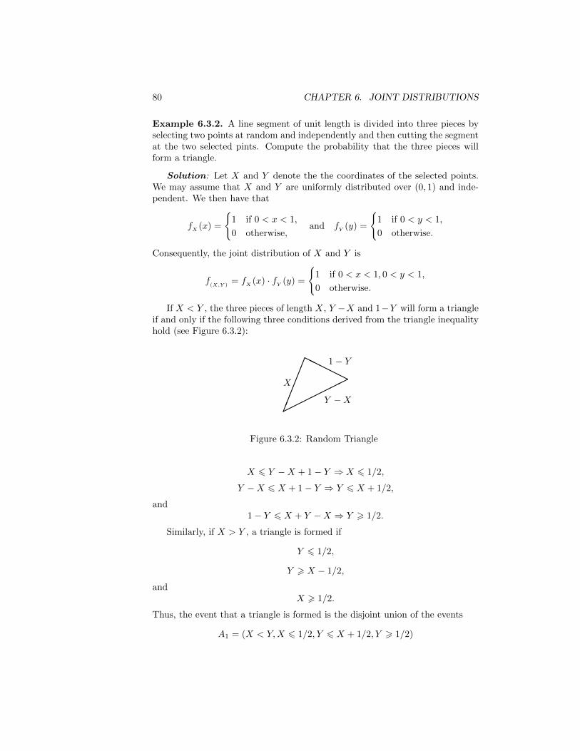
80 CHAPTER 6. JOINT DISTRIBUTIONS
Example 6.3.2. A line segment of unit length is divided into three pieces byselecting two points at random and independently and then cutting the segmentat the two selected pints. Compute the probability that the three pieces willform a triangle.
Solution: Let X and Y denote the the coordinates of the selected points.We may assume that X and Y are uniformly distributed over (0, 1) and inde-pendent. We then have that
fX
(x) =
{1 if 0 < x < 1,
0 otherwise,and f
Y(y) =
{1 if 0 < y < 1,
0 otherwise.
Consequently, the joint distribution of X and Y is
f(X,Y )
= fX
(x) · fY
(y) =
{1 if 0 < x < 1, 0 < y < 1,
0 otherwise.
If X < Y , the three pieces of length X, Y −X and 1−Y will form a triangleif and only if the following three conditions derived from the triangle inequalityhold (see Figure 6.3.2):
�����
��HH
HHH�
�����
1− Y
X
Y −X
Figure 6.3.2: Random Triangle
X 6 Y −X + 1− Y ⇒ X 6 1/2,
Y −X 6 X + 1− Y ⇒ Y 6 X + 1/2,
and1− Y 6 X + Y −X ⇒ Y > 1/2.
Similarly, if X > Y , a triangle is formed if
Y 6 1/2,
Y > X − 1/2,
andX > 1/2.
Thus, the event that a triangle is formed is the disjoint union of the events
A1 = (X < Y,X 6 1/2, Y 6 X + 1/2, Y > 1/2)
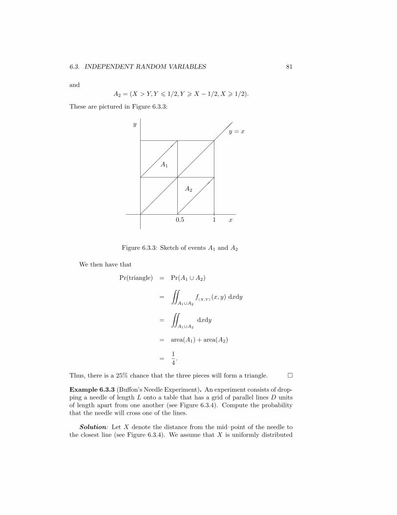
6.3. INDEPENDENT RANDOM VARIABLES 81
and
A2 = (X > Y, Y 6 1/2, Y > X − 1/2, X > 1/2).
These are pictured in Figure 6.3.3:
x
y
10.5���������������y = x
������
A1
������
A2
Figure 6.3.3: Sketch of events A1 and A2
We then have that
Pr(triangle) = Pr(A1 ∪A2)
=
∫∫A1∪A2
f(X,Y )
(x, y) dxdy
=
∫∫A1∪A2
dxdy
= area(A1) + area(A2)
=1
4.
Thus, there is a 25% chance that the three pieces will form a triangle. �
Example 6.3.3 (Buffon’s Needle Experiment). An experiment consists of drop-ping a needle of length L onto a table that has a grid of parallel lines D unitsof length apart from one another (see Figure 6.3.4). Compute the probabilitythat the needle will cross one of the lines.
Solution: Let X denote the distance from the mid–point of the needle tothe closest line (see Figure 6.3.4). We assume that X is uniformly distributed
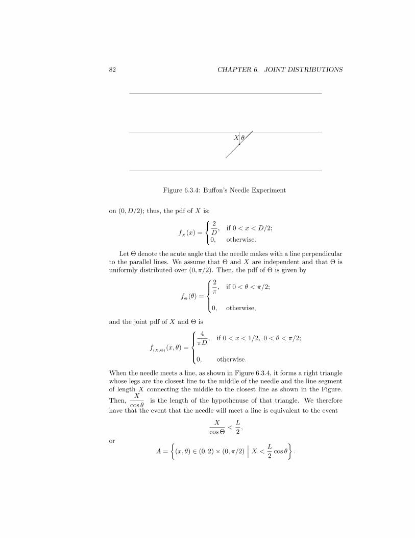
82 CHAPTER 6. JOINT DISTRIBUTIONS
�����qX θ
Figure 6.3.4: Buffon’s Needle Experiment
on (0, D/2); thus, the pdf of X is:
fX
(x) =
2
D, if 0 < x < D/2;
0, otherwise.
Let Θ denote the acute angle that the needle makes with a line perpendicularto the parallel lines. We assume that Θ and X are independent and that Θ isuniformly distributed over (0, π/2). Then, the pdf of Θ is given by
fΘ
(θ) =
2
π, if 0 < θ < π/2;
0, otherwise,
and the joint pdf of X and Θ is
f(X,Θ)
(x, θ) =
4
πD, if 0 < x < 1/2, 0 < θ < π/2;
0, otherwise.
When the needle meets a line, as shown in Figure 6.3.4, it forms a right trianglewhose legs are the closest line to the middle of the needle and the line segmentof length X connecting the middle to the closest line as shown in the Figure.
Then,X
cos θis the length of the hypothenuse of that triangle. We therefore
have that the event that the needle will meet a line is equivalent to the event
X
cos Θ<L
2,
or
A =
{(x, θ) ∈ (0, 2)× (0, π/2)
∣∣∣ X <L
2cos θ
}.

6.3. INDEPENDENT RANDOM VARIABLES 83
We then have that the probability that the needle meets a line is
Pr(A) =
∫∫A
f(X,Θ)
(x, θ) dxdθ
=
∫ π/2
0
∫ L cos(θ)/2
0
4
πDdxdθ
=2L
πD
∫ π/2
0
cos θ dθ
=2L
πDsin θ
∣∣∣π/20
=2L
πD.
Thus, in the case in which D = L, there is a 2/π, or about 64%, chance thatthe needle will meet a line. �
Example 6.3.4 (Infinite two–dimensional target). Place the center of a targetfor a darts game at the origin of the xy–plane. If a dart lands at a point withcoordinates (X,Y ), then the random variables X and Y measure the horizontaland vertical miss distance, respectively. For instance, if X < 0 and Y > 0 , then
rx
y
(X,Y )r
Figure 6.3.5: xy–target
the dart landed to the left of the center at a distance |X| from a vertical linegoing through the origin, and at a distance Y above the horizontal line goingthrough the origin (see Figure 6.3.5).
We assume that X and Y are independent, and we are interested in findingthe marginal pdfs f
Xand f
Yof X and Y , respectively.
84 CHAPTER 6. JOINT DISTRIBUTIONS
Assume further that the joint pdf of X and Y is given by the functionf(x, y), and that it depends only on the distance from (X,Y ) to the origin.More precisely, we suppose that
f(x, y) = g(x2 + y2) for all (x, y) ∈ R2,
where g is a differentiable function of a single variable. This implies that
g(t) > 0 for all t > 0,
and ∫ ∞0
g(t) dt =1
π. (6.4)
This follows from the fact that f is a pdf and therefore∫∫R2
f(x, y) dxdy = 1.
Thus, switching to polar coordinates,
1 =
∫ 2π
0
∫ ∞0
g(r2)r ddθ.
Hence, after making the change of variables t = r2, we get that
1 = 2π
∫ ∞0
g(r2) rdr = π
∫ ∞0
g(t) dt,
from which (6.4) follows.Now, since we are assuming that X and Y are independent, it follows that
f(x, y) = fX
(x) · fY
(y) for all (x, y) ∈ R2.
ThusfX(x) · fY (y) = g(x2 + y2).
Differentiating with respect to x, we get
f ′X
(x) · fY
(y) = g′(x2 + y2) · 2x.
Dividing this equation by x · fX
(x) · fY
(y) = x · g(x2 + y2), we get
1
x·f ′X
(x)
fX
(x)=
2g′(x2 + y2)
g(x2 + y2)for all (x, y) ∈ R2
with (x, y) 6= (0, 0).Observe that the left–hand side of the equation is a function of x, while the
right hand side is a function of both x and y. It follows that the left-hand-sidemust be constant. The reason for this is that, by symmetry,
2g′(x2 + y2
g(x2 + y2)=
1
y
f ′Y
(y)
fY
(y)
6.3. INDEPENDENT RANDOM VARIABLES 85
So that,1
x
f ′X
(x)
fX
(x)=
1
y
f ′Y
(y)
fY
(y)
for all (x, y) ∈ R2, (x, y) 6= (0, 0. Thus, in particular
1
x
f ′X
(x)
fX
(x)=f ′Y
(1)
fY
(1)= a, for all x ∈ R,
and some constant a. It then follows that
f ′X
(x)
fX
(x)= ax
for all x ∈ R. We therefore get that
d
dx
[ln(f
X(x))
]= ax.
Integrating with respect to x, we then have that
ln(fX
(x))
= ax2
2+ c1,
for some constant of integration c1. Thus, exponentiating on both sides of theequation we get that
fX
(x) = cea2 x
2
for all x ∈ R.
Thus fX
(x) must be a multiple of ea2 x
2
. Now, for this to be a pdf , we must havethat ∫ ∞
−∞fX
(x) dx = 1.
Then, necessarily, it must be the case that a < 0 (Why?). Say, a = −δ2, then
fX
(x) = ce−δ2
2 x2
To determine what the constant c should be, we use the condition∫ ∞−∞
fX
(x) dx = 1.
Let
I =
∫ ∞−∞
e−δ2x2/2 dx.
Observe that
I =
∫ ∞−∞
e−δ2y2/2 dy.
86 CHAPTER 6. JOINT DISTRIBUTIONS
We then have that
I2 =
∫ ∞−∞
e−δ2 x2
2 dx ·∫ ∞−∞
e−δ2 y2
2 dy
=
∫ ∞−∞
∫ ∞−∞
e−δ2
2 (x2+y2) dxdy.
Switching to polar coordinates we get
I2 =
∫ 2π
0
∫ ∞0
e−δ2
2 r2
r drdθ
=2π
δ2
∫ ∞0
e−u du
=2π
δ2,
where we have also made the change of variables u =δ2
2r2. Thus, taking the
square root,
I =
√2π
δ.
Hence, the condition ∫ ∞−∞
fX
(x)dx = 1
implies that
c
√2π
δ= 1
from which we get that
c =δ√2π
Thus, the pdf for X is
fX
(x) =δ√2πe−
δ2x2
2 for all x ∈ R.
Similarly, or by using symmetry, we obtain that the pdf for Y is
fY
(y) =δ√2πe−
δ2y2
2 for all y ∈ R.
That is, X and Y have the same distribution.
6.3. INDEPENDENT RANDOM VARIABLES 87
We next set out to compute the expected value and variance of X. In orderto do this, we first compute the moment generating function, ψ
X(t), of X:
ψX
(t) = E(etX)
=δ√2π
∫ ∞−∞
etxe−δ2x2
2 dx
=δ√2π
∫ ∞−∞
e−δ2x2
2 +tx dx
=δ√2π
∫ ∞−∞
e−δ2
2 (x2− 2txδ2
) dx
Complete the square on x to get
x2 − 2t
δ2x = x2 − 2t
δ2x+
t2
δ4− t2
δ4=
(x− t
δ2
)2
− t2
δ4;
then,
ψX
(t) =δ√2π
∫ ∞−∞
e−δ2
2 (x− tδ2
)2
et2/2δ2
dx
= et2/2δ2 δ√
2π
∫ ∞−∞
e−δ2
2 (x− tδ2
)2
dx.
Make the change of variables
u = x− t
δ2
then du = dx and
ψX
(t) = et2
2δ2δ√2π
∫ ∞−∞
e−δ2
2 u2
du
= et2
2δ2 ,
since, as we have previously seen in this example,
f(u) =δ√2πe−δ2
2 u2
, for u ∈ R,
is a pdf and therefore ∫ ∞−∞
δ√2πe−δ2
2 u2
du = 1.
Hence, the mgf of X is
ψX
(t) = et2
2δ2 for all t ∈ R.
Differentiating with respect to t we obtain
ψ′X
(t) =t
δ2et2
2δ2
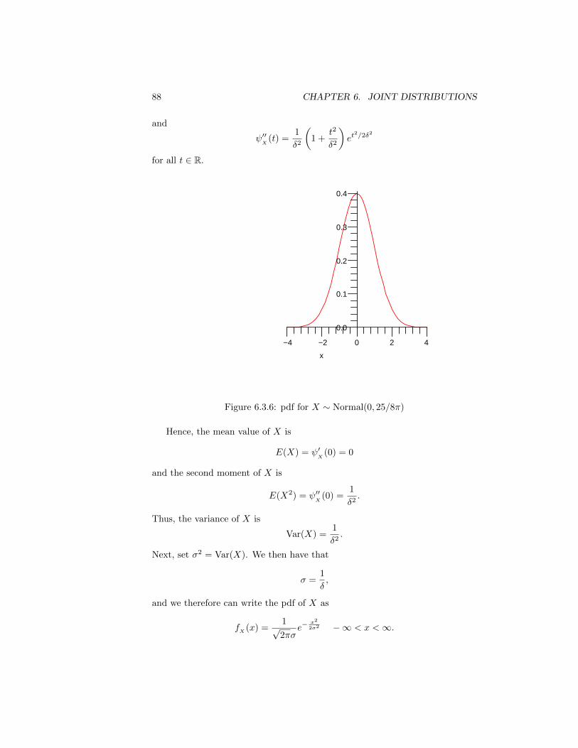
88 CHAPTER 6. JOINT DISTRIBUTIONS
and
ψ′′X
(t) =1
δ2
(1 +
t2
δ2
)et
2/2δ2
for all t ∈ R.
2
0.3
0.1
−2
x
4
0.4
0.2
0
0.0
−4
Figure 6.3.6: pdf for X ∼ Normal(0, 25/8π)
Hence, the mean value of X is
E(X) = ψ′X
(0) = 0
and the second moment of X is
E(X2) = ψ′′X
(0) =1
δ2.
Thus, the variance of X is
Var(X) =1
δ2.
Next, set σ2 = Var(X). We then have that
σ =1
δ,
and we therefore can write the pdf of X as
fX
(x) =1√2πσ
e−x2
2σ2 −∞ < x <∞.
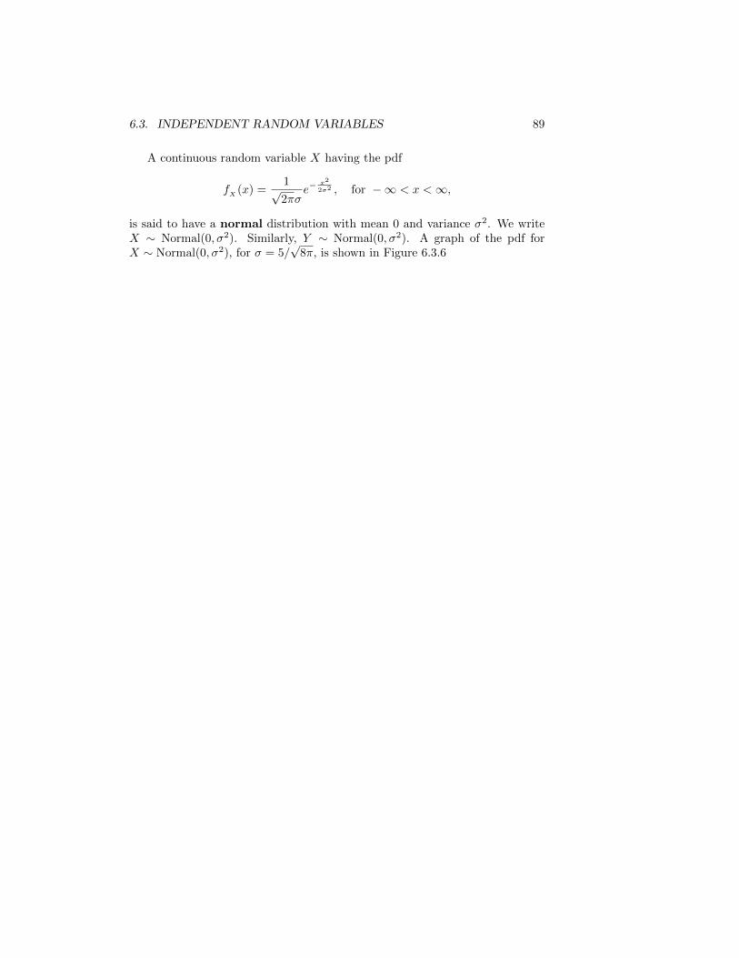
6.3. INDEPENDENT RANDOM VARIABLES 89
A continuous random variable X having the pdf
fX
(x) =1√2πσ
e−x2
2σ2 , for −∞ < x <∞,
is said to have a normal distribution with mean 0 and variance σ2. We writeX ∼ Normal(0, σ2). Similarly, Y ∼ Normal(0, σ2). A graph of the pdf forX ∼ Normal(0, σ2), for σ = 5/
√8π, is shown in Figure 6.3.6

90 CHAPTER 6. JOINT DISTRIBUTIONS

Chapter 7
Some Special Distributions
In this notes and in the exercises we have encountered several special kindsof random variables and their respective distribution functions in the contextof various examples and applications. For example, we have seen the uniformdistribution over some interval (a, b) in the context of medeling the selection ofa point in (a, b) at random, and the exponential distribution comes up whenmodeling the service time at a checkout counter. We have discussed Bernoullitrials and have seen that the sum of independent Bernoulli trials gives rise tothe Binomial distribution. In the exercises we have seen the discrete uniformdistribution, the geometric distribution and the hypergeometric distribution.More recently, in the last example of the previous section, we have seen thatthe miss horizontal distance from the y–axis of dart that lands in an infinitetarget follows a Normal(0, σ2) distribution (assuming that the miss horizontaland vertical distances are independent and that their joint pdf is radially sym-metric). In the next section we discuss the normal distribution in more detail.In subsequent sections we discuss other distributions which come up frequentlyin application, such as the Poisson distribution.
7.1 The Normal Distribution
In Example 6.3.4 we saw that if X denotes the horizontal miss distance fromthe y–axis of a dart that lands on an infinite two–dimensional target, the X hasa pdf given by
fX
(x) =1√2πσ
e−x2
2σ2 , for −∞ < x <∞,
for some constant σ > 0. In the derivation in Example 6.3.4 we assumed thatthe X is independent from the Y coordinate (or vertical miss distance) of thepoint where the dart lands, and that the joint distribution of X and Y dependsonly on the distance from that point to the origin. We say that X has a normaldistribution with mean 0 and variance σ2. More generally,we have the followingdefinition:
91
92 CHAPTER 7. SOME SPECIAL DISTRIBUTIONS
Definition 7.1.1 (Normal Distribution). A continuous random variable, X,with pdf
fX
(x) =1√2πσ
e−(x−µ)2
2σ2 , for −∞ < x <∞,
and parameters µ and σ2, where µ ∈ R and σ > 0, is said to have a normaldistribution with parameters µ and σ2. We write X ∼ Normal(µ, σ2)
The special random variable Z ∼ Normal(0, 1) has a distribution functionknown as the standard normal distribution:
fZ
(z) =1√2π
e−z2/2 for −∞ < z <∞. (7.1)
From the calculations in Example 6.3.4 we get that the moment generatingfunction for Z is
ψZ
(t) = et2/2 for −∞ < t <∞. (7.2)
Example 7.1.2. Let µ ∈ R and σ > 0 be given, and define
X = σZ + µ.
Show that X ∼ Normal(µ, σ2) and compute the moment generating function ofX, its expectation and its variance.
Solution: First we find the pdf of X and show that it is the same as thatgiven in Definition 7.1.1. In order to do this, we first compute the cdf of X:
FX
(x) = Pr(X 6 x)= Pr(σZ + µ 6 x)= Pr[Z 6 (x− µ)/σ]= F
Z((x− µ)/σ).
Differentiating with respect to x, while remembering to use the Chain Rule, weget that
fX
(x) = F ′Z
((x− µ)/σ) · (1/σ)
=1
σfZ
(x− µσ
).
Thus, using (7.1), we get
fX
(x) =1
σ· 1√
2πe−[(x−µ)/σ]2/2
=1√2πσ
e−(x−µ)2
2σ2 ,
for −∞ < x <∞, which is the pdf for a Normal(µ, σ2) random variable accord-ing to Definition 7.1.1.
7.1. THE NORMAL DISTRIBUTION 93
Next, we compute the mgf of X:
ψX
(t) = E(etX)= E(et(σZ+µ))= E(etσZ+tµ)= E(eσtZeµt)= eµtE(e(σt)Z)= eµtψ
Z(σt),
for −∞ < t <∞. It then follows from (7.2) that
ψX
(t) = eµte(σt)2/2
= eµteσ2t2/2
= eµt+σ2t2/2,
for −∞ < t <∞.Differentiating with respect to t, we obtain
ψ′X
(t) = (µ+ σ2t)eµt+σ2t2/2
andψ′′X
(t) = σ2eµt+σ2t2/2 + (µ+ σ2t)2eµt+σ
2t2/2
for −∞ < t <∞.Consequently, the expected value of X is
E(X) = ψ′X
(0) = µ,
and the second moment of X is
E(X2) = ψ′′X
(0) = σ2 + µ2.
Thus, the variance of X is
Var(X) = E(X2)− µ2 = σ2.
We have therefore shown that if X ∼ Normal(µ, σ2), then the parameter µ isthe mean of X and σ2 is the variance of X. �
Example 7.1.3. Suppose that many observations from a Normal(µ, σ2) distri-bution are made. Estimate the proportion of observations that must lie withinone standard deviation from the mean.
Solution: We are interested in estimating Pr(|X − µ| < σ), where X ∼Normal(µ, σ2).
Compute
Pr(|X − µ| < σ) = Pr(−σ < X − µ < σ)
= Pr
(−1 <
X − µσ
< 1
),

94 CHAPTER 7. SOME SPECIAL DISTRIBUTIONS
where, according to Problem (1) in Assignment #16,
X − µσ
∼ Normal(0, 1);
that is, it has a standard normal distribution. Thus, setting
Z =X − µσ
,
we get thatPr(|X − µ| < σ) = Pr(−1 < Z < 1),
where Z ∼ Normal(0, 1). Observe that
Pr(|X − µ| < σ) = Pr(−1 < Z < 1)= Pr(−1 < Z 6 1)= F
Z(1)− F
Z(−1),
where FZ
is the cdf of Z. MS Excel has a built in function called normdist whichreturns the cumulative distribution function value at x, from a Normal(µ, σ2)random variable, X, given x, the mean µ, the standard deviation σ and a“TRUE” tag as follows:
FZ
(z) = normdist(z, µ, σ,TRUE) = normdist(z, 0, 1,TRUE).
We therefore obtain the approximation
Pr(|X − µ| < σ) ≈ 0.8413− 0.1587 = 0.6826, or about 68%.
Thus, around 68% of observations from a normal distribution should lie withinone standard deviation from the mean. �
Example 7.1.4 (The Chi–Square Distribution with one degree of freedom).Let Z ∼ Normal(0, 1) and define Y = Z2. Give the pdf of Y .
Solution: The pdf of Z is given by
fX
(z) =1√2πe−z
2/2, for −∞ < z <∞.
We compute the pdf for Y by first determining its cdf:
P (Y ≤ y) = P (Z2 ≤ y) for y > 0
= P (−√y ≤ Z ≤ √y)
= P (−√y < Z ≤ √y), since Z is continuous.
Thus,
P (Y ≤ y) = P (Z ≤ √y)− P (Z ≤ −√y)
= FZ
(√y)− F
Z(−√y) for y > 0,
7.1. THE NORMAL DISTRIBUTION 95
since Y is continuous.We then have that the cdf of Y is
FY
(y) = FZ
(√y)− F
Z(−√y) for y > 0,
from which we get, after differentiation with respect to y,
fY
(y) = F ′Z
(√y) · 1
2√y
+ F ′Z
(−√y) · 1
2√y
= fZ
(√y)
1
2√y
+ fZ
(−√y)1
2√y
=1
2√y
{1√2π
e−y/2 +1√2π
e−y/2}
=1√2π· 1√ye−y/2
for y > 0. �
Definition 7.1.5. A continuous random variable Y having the pdf
fY
(y) =
1√2π· 1√ye−y/2 if y > 0
0 otherwise,
is said to have a Chi–Square distribution with one degree of freedom. We write
Y ∼ χ21.
Remark 7.1.6. Observe that if Y ∼ χ21, then its expected value is
E(Y ) = E(Z2) = 1.
To compute the second moment of Y , E(Y 2) = E(Z4), we need to compute thefourth moment of Z. Recall that the mgf of Z is
ψZ
(t) = et2/2 for all t ∈ R.
Its fourth derivative can be computed to be
ψ(4)Z
(t) = (3 + 6t2 + t4) et2/2 for all t ∈ R.
Thus,E(Z4) = ψ(4)
Z(0) = 3.
We then have that the variance of Y is
Var(Y ) = E(Y 2)− 1 = E(Z4)− 1 = 3− 1 = 2.
96 CHAPTER 7. SOME SPECIAL DISTRIBUTIONS
7.2 The Poisson Distribution
Example 7.2.1 (Bacterial Mutations). Consider a colony of bacteria in a cul-ture consisting of N bacteria. This number, N , is typically very large (in theorder of 106 bacteria). We consider the question of how many of those bacteriawill develop a specific mutation in their genetic material during one divisioncycle (e.g., a mutation that leads to resistance to certain antibiotic or virus).We assume that each bacterium has a very small, but positive, probability, a, ofdeveloping that mutation when it divides. This probability is usually referredto as the mutation rate for the particular mutation and organism. If we letXN denote the number of bacteria, out of the N in the colony, that develop themutation in a division cycle, we can model XN by a binomial random variablewith parameters a and N ; that is,
XN ∼ Binomial(N, a).
This assertion is justified by assuming that the event that a given bacteriumdevelops a mutation is independent of any other bacterium in the colony devel-oping a mutation. We then have that
Pr(XN = k) =
(N
k
)ak(1− a)N−k, for k = 0, 1, 2, . . . , N. (7.3)
Also,
E(XN ) = aN.
Thus, the average number of mutations in a division cycle is aN . We will denotethis number by λ and will assume that it remains constant; that is,
aN = λ (a constant.)
Since N is very large, it is reasonable to make the approximation
Pr(XN = k) ≈ limN→∞
(N
k
)ak(1− a)N−k, for k = 0, 1, 2, 3, . . .
provided that the limit on the right side of the expression exists. In this examplewe show that the limit in the expression above exists if aN = λ is kept constantas N tends to infinity. To see why this is the case, we first substitute λ/N fora in the expression for Pr(XN = k) in equation (7.3). We then get that
Pr(XN = k) =
(N
k
)(λ
N
)k (1− λ
N
)N−k,
which can be re-written as
Pr(XN = k) =λk
k!· N !
(N − k)!· 1
Nk·(
1− λ
N
)N·(
1− λ
N
)−k. (7.4)
7.2. THE POISSON DISTRIBUTION 97
Observe that
limN→∞
(1− λ
N
)N= e−λ, (7.5)
since limn→∞
(1 +
x
n
)n= ex for all real numbers x. Also note that, since k is
fixed,
limN→∞
(1− λ
N
)−k= 1. (7.6)
It remains to see then what happens to the termN !
(N − k)!· 1
Nk, in equation
(7.4), as N →∞. To answer this question, we compute
N !
(N − k)!· 1
Nk=
N(N − 1)(N − 2) · · · (N − (k − 1))
Nk
=
(1− 1
N
)(1− 2
N
)· · ·(
1− k − 1
N
).
Thus, since
limN→∞
(1− j
N
)= 1 for all j = 1, 2, 3, . . . , k − 1,
it follows that
limN→∞
N !
(N − k)!· 1
Nk= 1. (7.7)
Hence, in view of equations (7.5), (7.6) and (7.7), we see from equation (7.4)that
limN→∞
Pr(XN = k) =λk
k!e−λ for k = 0, 1, 2, 3, . . . . (7.8)
The limiting distribution obtained in equation (7.8) is known as the Poissondistribution with parameter λ. We have therefore shown that the number ofmutations occurring in a bacterial colony of size N , per division cycle, can beapproximated by a Poisson random variable with parameter λ = aN , where ais the mutation rate.
Definition 7.2.2 (Poisson distribution). A discrete random variable, X, withpmf
pX
(k) =λk
k!e−λ for k = 0, 1, 2, 3, . . . ; zero elsewhere,
where λ > 0, is said to have a Poisson distribution with parameter λ. We writeX ∼ Poisson(λ).
To see that the expression for pX
(k) in Definition 7.2.2 indeed defines a pmf,observe that
∞∑k=0
λk
k!= eλ,
98 CHAPTER 7. SOME SPECIAL DISTRIBUTIONS
from which we get that
∞∑k=0
pX
(k) =
∞∑k=0
λk
k!e−λ = eλ · e−λ = 1.
In a similar way we can compute the mgf of X ∼ Poisson(λ) to obtain (seeProblem 1 in Assignment #19):
ψX
(t) = eλ(et−1) for all t ∈ R.
Using this mgf we can derive that the expected value of X ∼ Poisson(λ) is
E(X) = λ,
and its variance isVar(X) = λ
as well.
Example 7.2.3 (Sum of Independent Poisson Random Variables). Supposethat X ∼ Poisson(λ1) and Y ∼ Poisson(λ2) are independent random variables,where λ1 and λ2 are positive. Define Z = X + Y . Give the distribution of Z.
Solution: Use the independence of X and Y to compute the mgf of Z:
ψZ
(t) = ψX+Y
(t)= ψ
X(t) · ψ
Y(t)
= eλ1(et−1) · eλ2(et−1)
= e(λ1+λ2)(et−1),
which is the mgf of a Poisson(λ1 + λ2) distribution. It then follows that
Z ∼ Poisson(λ1 + λ2)
and therefore
pZ
(k) =(λ1 + λ2)k
k!e−λ1−λ2 for k = 0, 1, 2, 3, . . . ; zero elsewhere.
�
Example 7.2.4 (Estimating Mutation Rates in Bacterial Populations). Luriaand Delbruck1 devised the following procedure (known as the fluctuation test)to estimate the mutation rate, a, for certain bacteria:Imagine that you start with a single normal bacterium (with no mutations) andallow it to grow to produce several bacteria. Place each of these bacteria intest–tubes each with media conducive to growth. Suppose the bacteria in thetest–tubes are allowed to reproduce for n division cycles. After the nth division
1(1943) Mutations of bacteria from virus sensitivity to virus resistance. Genetics, 28,491–511
7.2. THE POISSON DISTRIBUTION 99
cycle, the content of each test–tube is placed onto a agar plate containing avirus population which is lethal to the bacteria which have not developed resis-tance. Those bacteria which have mutated into resistant strains will continue toreplicate, while those that are sensitive to the virus will die. After certain time,the resistant bacteria will develop visible colonies on the plates. The number ofthese colonies will then correspond to the number of resistant cells in each testtube at the time they were exposed to the virus. This number corresponds tothe number of bacteria in the colony that developed a mutation which led toresistance. We denote this number by XN , as we did in Example 7.2.1, where Nis the size of the colony after the nth division cycle. Assuming that the bacteriamay develop mutation to resistance after exposure to the virus, the argumentin Example 7.2.1 shows that, if N is very large, the distribution of XN canbe approximated by a Poisson distribution with parameter λ = aN , where ais the mutation rate and N is the size of the colony. It then follows that theprobability of no mutations occurring in one division cycle is
Pr(XN = 0) ≈ e−λ. (7.9)
This probability can also be estimated experimentally as Luria and nd Delbruckshowed in their 1943 paper. In one of the experiments described in that paper,out of 87 cultures of 2.4×10⁸ bacteria, 29 showed not resistant bacteria (i.e., noneof the bacteria in the culture mutated to resistance and therefore all perishedafter exposure to the virus). We therefore have that
Pr(XN = 0) ≈ 29
87.
Comparing this to the expression in Equation (7.9), we obtain that
e−λ ≈ 29
87,
which can be solved for λ to obtain
λ ≈ − ln
(29
87
)or
λ ≈ 1.12.
The mutation rate, a, can then be estimated from λ = aN :
a =λ
N≈ 1.12
2.4× 10⁸≈ 4.7× 10⁻⁹.

100 CHAPTER 7. SOME SPECIAL DISTRIBUTIONS

Chapter 8
Convergence in Distribution
We have seen in Example 7.2.1 that if Xn ∼ Binomial(λ/n, n), for some constantλ > 0 and n = 1, 2, 3, . . ., and if Y ∼ Poisson(λ), then
limn→∞
Pr(Xn = k) = Pr(Y = k) for all k = 0, 1, 2, 3, . . .
We then say that the sequence of Binomial random variables (X1, X2, X3, . . .)converges in distribution to the Poisson random variable Y with parameterλ. This concept will be made more general and precise in the following section.
8.1 Definition of Convergence in Distribution
Definition 8.1.1 (Convergence in Distribution). Let (Xn) be a sequence ofrandom variables with cumulative distribution functions F
Xn, for n = 1, 2, 3, . . .,
and Y be a random variable with cdf FY
. We say that the sequence (Xn)converges to Y in distribution, if
limn→∞
FXn
(x) = FY
(x)
for all x where FY
is continuous.We write
XnD→ Y as n→∞.
Thus, if (Xn) converges to Y in distribution then
limn→∞
Pr(Xn 6 x) = Pr(Y 6 x) for x at which FY
is continuous.
If Y is discrete, for instance taking on nonzero values at k = 0, 1, 2, 3, . . . (asis the case with the Poisson distribution), then F
Yis continuous in between
consecutive integers k and k+1. We therefore get that for any ε with 0 < ε < 1,
limn→∞
Pr(Xn 6 k + ε) = Pr(Y 6 k + ε)
101
102 CHAPTER 8. CONVERGENCE IN DISTRIBUTION
for all k = 0, 1, 2, 3, . . .. Similarly,
limn→∞
Pr(Xn 6 k − ε) = Pr(Y 6 k − ε)
for all k = 0, 1, 2, 3, . . .. We therefore get that
limn→∞
Pr(k − ε < Xn 6 k + ε) = Pr(k − ε < Y 6 k + ε)
for all k = 0, 1, 2, 3, . . .. From this we get that
limn→∞
Pr(Xn = k) = Pr(Y = k)
for all k = 0, 1, 2, 3, . . ., in the discrete case.
If (Xn) converges to Y in distribution and the moment generating functionsψXn
(t) for n = 1, 2, 3 . . ., and ψY
(t) all exist on some common interval of valuesof t, then it might be the case, under certain technical conditions which may befound in a paper by Kozakiewicz,1 that
limn→∞
ψXn
(t) = ψY
(t)
for all t in the common interval of existence.
Example 8.1.2. Let Xn ∼ Binomial(λ/n, n) for n = 1, 2, 3, . . ..
ψXn
(t) =
(λet
n+ 1− λ
n
)nfor all n and all t.
Then,
limn→∞
ψXn
(t) = limn→∞
(1 +
λ(et − 1)
n
)n= eλ(et−1),
which is the moment generating function of a Poisson(λ) distribution. This isnot surprising since we already know that Xn converges to Y ∼ Poisson(λ) indistribution. What is surprising is the theorem discussed in the next sectionknown as the mgf Convergence Theorem.
8.2 mgf Convergence Theorem
Theorem 8.2.1 (mgf Convergence Theorem, Theorem 5.7.4 on page 289 inthe text). Let (Xn) be a sequence of random variables with moment generat-ing functions ψ
Xn(t) for |t| < h, n = 1, 2, 3, . . ., and some positive number h.
Suppose Y has mgf ψY
(t) which exists for |t| < h. Then, if
limn→∞
ψXn
(t) = ψY
(t), for |t| < h,
it follows thatlimn→∞
FXn
(x) = FY
(x)
for all x where FY is continuous.
1(1947) On the Convergence of Sequences of Moment Generating Functions. Annals ofMathematical Statistics, Volume 28, Number 1, pp. 61–69
8.2. MGF CONVERGENCE THEOREM 103
Notation. If (Xn) converges to Y in distribution as n tends to infinity, wewrite
XnD−→ Y as n→∞.
The mgf Convergence Theorem then says that if the moment generatingfunctions of a sequence of random variables, (Xn), converges to the mgf ofa ranfom variable Y on some interval around 0, the Xn converges to Y indistribution as n→∞.
The mgf Theorem is usually ascribed to Levy and Cramer (c.f. the paperby Curtiss2)
Example 8.2.2. Let X1, X2, X3, . . . denote independent, Poisson(λ) randomvariables. For each n = 1, 2, 3, . . ., define the random variable
Xn =X1 +X2 + · · ·+Xn
n.
Xn is called the sample mean of the random sample of size n, {X1, X2, . . . , Xn}.
The expected value of the sample mean, Xn, is obtained from
E(Xn) = E
(1
n(X1 +X2 + · · ·+Xn)
)
=1
n
n∑k=1
E(Xk)
=1
n
n∑k=1
λ
=1
n(nλ)
= λ.
2(1942) A note on the Theory of Moment Generating Functions. Annals of MathematicalStatistics, Volume 13, Number 4, pp. 430–433

104 CHAPTER 8. CONVERGENCE IN DISTRIBUTION
Since the Xi’s are independent, the variance of Xn can be computed as follows
Var(Xn) = Var
(1
n(X1 +X2 + · · ·+Xn)
)
=1
n2
n∑k=1
Var(Xk)
=1
n2
n∑k=1
λ
=1
n2(nλ)
=λ
n.
We can also compute the mgf of Xn as follows:
ψXn
(t) = E(etXn)
= ψX1+X2+···+Xn
(t
n
)
= ψX1
(t
n
)ψX2
(t
n
)· · ·ψ
Xn
(t
n
),
since the Xi’s are linearly independent. Thus, given the Xi’s are identicallydistributed Poisson(λ),
ψXn
(t) =
[ψX1
(t
n
)]n=
[eλ(et/n−1)
]n= eλn(et/n−1),
for all t ∈ R.Next we define the random variables
Zn =Xn − E(Xn)√
Var(Xn)=Xn − λ√λ/n
, for n = 1, 2, 3, . . .
We would like to see if the sequence of random variables (Zn) converges indistribution to a limiting random variable. To answer this question, we apply
8.2. MGF CONVERGENCE THEOREM 105
the mgf Convergence Theorem (Theorem 8.2.1). Thus, we compute the mgf ofZn for n = 1, 2, 3, . . .
ψZn
(t) = E(etZn)
= E
(et√n√λXn−t
√λn
)
= e−t√λn E
(et√n√λXn
)
= e−t√λn ψ
Xn
(t√n√λ
).
Next, use the fact that
ψXn
(t) = eλn(et/n−1),
for all t ∈ R, to get that
ψZn
(t) = e−t√λn eλn(e(t
√n/√λ)/n−1)
= e−t√λn eλn(et/
√λn−1).
Now, using the fact that
ex =
n∑k=0
xk
k!= 1 + x+
x2
2+x3
3!+x4
4!+ · · · ,
we obtain that
et/√nλ = 1 +
t√nλ
+1
2
t2
nλ+
1
3!
t3
nλ√nλ
+1
4!
t4
(nλ)2+ · · ·
so that
et/√nλ − 1 =
t√nλ
+1
2
t2
nλ+
1
3!
t3
nλ√nλ
+1
4!
t4
(nλ)2+ · · ·
and
λn(et/√nλ − 1) =
√nλt+
1
2t2 +
1
3!
t3
nλ+
1
4!
t4
nλ+ · · ·
Consequently,
eλn(et/√nλ−1) = e
√nλt · et
2/2 · e 13!
t3
nλ+ 14!
t4
nλ+···
and
e−√nλteλn(et/
√nλ−1) = et
2/2 · e 13!
t3
nλ+ 14!
t4
nλ+···.
106 CHAPTER 8. CONVERGENCE IN DISTRIBUTION
Observe that the exponent in the last exponential tends to 0 as n → ∞. Wetherefore get that
limn→∞
[e−√nλteλn(et/
√nλ−1)
]= et
2/2 · e0 = et2/2.
We have thus shown that
limn→∞
ψZn
(t) = et2/2, for all t ∈ R,
where the right–hand side is the mgf of Z ∼ Normal(0, 1). Hence, by the mgfConvergence Theorem, Zn converges in distribution to a Normal(0, 1) randomvariable.
Example 8.2.3 (Estimating Proportions). Suppose we sample from a givenvoting population by surveying a random group of n people from that popu-lation and asking them whether or not they support certain candidate. In thepopulation (which could consists of hundreds of thousands of voters) there is aproportion, p, of people who support the candidate, and which is not known withcertainty. If we denote the responses of the surveyed n people byX1, X2, . . . , Xn,then we can model these responses as independent Bernoulli(p) random vari-ables: a responses of “yes” corresponds to Xi = 1, while Xi = 0 is a “no.” Thesample mean,
Xn =X1 +X2 + · · ·+Xn
n,
give the proportion of individuals from the sample who support the candidate.Since E(Xi) = p for each i, the expected value of the sample mean is
E(Xn) = p.
Thus, Xn can be used as an estimate for the true proportion, p, of people whosupport the candidate. How good can this estimate be? In this example we tryto answer this question.
By independence of the Xi’s, we get that
Var(Xn) =1
nVar(X1) =
p(1− p)n
.
8.2. MGF CONVERGENCE THEOREM 107
Also, the mgf of Xn is given by
ψXn
(t) = E(etXn)
= ψX1+X2+···+Xn
(t
n
)
= ψX1
(t
n
)ψX2
(t
n
)· · ·ψ
Xn
(t
n
)
=
[ψX1
(t
n
)]n=
(p et/n + 1− p
)n.
As in the previous example, we define the random variables
Zn =Xn − E(Xn)√
Var(Xn)=
Xn − p√p(1− p)/n
, for n = 1, 2, 3, . . . ,
or
Zn =
√n√
p(1− p)Xn −
√np
1− p, for n = 1, 2, 3, . . . .
Thus, the mgf of Zn is
ψZn
(t) = E(etZn)
= E
(e
t√n√
p(1−p)Xn−t
√np
1−p
)
= e−t√
np1−p E
(e
t√n√
p(1−p)Xn)
= e−t√
np1−p ψ
Xn
(t√n√
p(1− p)
)
= e−t√
np1−p
(p e(t
√n/√p(1−p)/n + 1− p
)n= e−t
√np
1−p
(p e(t/
√np(1−p) + 1− p
)n=
[e−tp
√1
np(1−p)
(p e(t/
√np(1−p)) + 1− p
)]n=
(p et(1−p)/
√np(1−p)) + (1− p)etp/
√np(1−p))
)n.
108 CHAPTER 8. CONVERGENCE IN DISTRIBUTION
To compute the limit of ψZn
(t) as n → ∞, we first compute the limit of
ln(ψZn
(t))
as n→∞, where
ln(ψZn
(t))
= n ln(p et(1−p)/
√np(1−p)) + (1− p)e−tp/
√np(1−p))
)= n ln
(p ea/
√n + (1− p) e−b/
√n),
where we have set
a =(1− p)t√p(1− p)
and b =p t√
p(1− p).
Observe thatpa− (1− p)b = 0, (8.1)
andp a2 + (1− p)b2 = (1− p)t2 + p t2 = t2. (8.2)
Writing
ln(ψZn
(t))
=ln(p ea/
√n + (1− p) e−b/
√n)
1
n
,
we see that L’Hospital’s Rule can be applied to compute the limit of ln(ψZn
(t))
as n→∞. We therefore get that
limn→∞
ln(ψZn
(t))
= limn→∞
−a21
n√np ea/
√n + b
21
n√n
(1− p) e−b/√n
p ea/√n + (1− p) e−b/
√n
− 1
n2
= limn→∞
a2
√np ea/
√n − b
2
√n(1− p) e−b/
√n
p ea/√n + (1− p) e−b/
√n
=1
2limn→∞
√n(ap ea/
√n − b(1− p) e−b/
√n)
p ea/√n + (1− p) e−b/
√n
.
Observe that the denominator in the last expression tends to 1 as n → ∞.Thus, if we can prove that the limit of the numerator exists, then the limit ofln(ψZn
(t))
will be 1/2 of that limit:
limn→∞
ln(ψZn
(t))
=1
2limn→∞
[√n(ap ea/
√n − b(1− p) e−b/
√n)]. (8.3)
The limit of the right–hand side of Equation (8.3) can be computed byL’Hospital’s rule by writing
√n(ap ea/
√n − b(1− p) e−b/
√n)
=ap ea/
√n − b(1− p) e−b/
√n
1√n
,
8.2. MGF CONVERGENCE THEOREM 109
and observing that the numerator goes to 0 as n tends to infinity by virtue ofEquation (8.1). Thus, we may apply L’Hospital’s Rule to obtain
limn→∞
√n(ap ea/
√n − b(1− p) e−b/
√n)
= limn→∞
− a2
2n√np ea/
√n − b2
2n√n
(1− p) e−b/√n
− 12n√n
= limn→∞
(a2p ea/
√n + b2(1− p) e−b/
√n)
= a2p+ b2(1− p)
= t2,
by Equation (8.2). It then follows from Equation (8.3) that
limn→∞
ln(ψZn
(t))
=t2
2.
Consequently, by continuity of the exponential function,
limn→∞
ψZn
(t) = limn→∞
eln(ψZn (t)) = et2/2,
which is the mgf of a Normal(0, 1) random variable. Thus, by the mgf Con-vergence Theorem, it follows that Zn converges in distribution to a standardnormal random variable. Hence, for any z ∈ R,
limn→∞
Pr
(Xn − p√p(1− p)/n
6 z
)= Pr (Z 6 z) ,
where Z ∼ Normal(0, 1). Similarly, with −z instead of z,
limn→∞
Pr
(Xn − p√p(1− p)/n
6 −z
)= Pr (Z 6 −z) .
It then follows that
limn→∞
Pr
(−z < Xn − p√
p(1− p)/n6 z
)= Pr (−z < Z 6 z) .
In a later example, we shall see how this information can be used provide a goodinterval estimate for the true proposition p.
The last two examples show that if X1, X2, X3, . . . are independent randomvariables which are distributed either Poisson(λ) or Bernoulli(p), then the ran-dom variables
Xn − E(Xn)√Var(Xn)
,
110 CHAPTER 8. CONVERGENCE IN DISTRIBUTION
where Xn denotes the sample mean of the random sample {X1, X2, . . . , Xn},for n = 1, 2, 3, . . ., converge in distribution to a Normal(0, 1) random variable;that is,
Xn − E(Xn)√Var(Xn)
D−→ Z as n→∞,
where Z ∼ Normal(0, 1). It is not a coincidence that in both cases we obtaina standard normal random variable as the limiting distribution. The examplesin this section are instances of general result known as the Central LimitTheorem to be discussed in the next section.
8.3 Central Limit Theorem
Theorem 8.3.1 (Central Limit Theorem). Suppose X1, X2, X3 . . . are inde-pendent, identically distributed random variables with E(Xi) = µ and finitevariance Var(Xi) = σ2, for all i. Then
Xn − µσ/√n
D−→ Z ∼ Normal(0, 1)
Thus, for large values of n, the distribution function forXn − µσ/√n
can be ap-
proximated by the standard normal distribution.
Proof. We shall prove the theorem for the special case in which the mgf of X1
exists is some interval around 0. This will allow us to use the mgf ConvergenceTheorem (Theorem 8.2.1).
We shall first prove the theorem for the case µ = 0. We then have that
ψ′X1
(0) = 0
and
ψ′′X1
(0) = σ2.
Let
Zn =Xn − µσ/√n
=
√n
σXn for n = 1, 2, 3, . . . ,
since µ = 0. Then, the mgf of Zn is
ψZn
(t) = ψXn
(t√n
σ
),
where the mgf of Xn is
ψXn
(t) =
[ψX1
(t
n
)]n,
8.3. CENTRAL LIMIT THEOREM 111
for all n = 1, 2, 3, . . . Consequently,
ψZn
(t) =
[ψX1
(t
σ√n
)]n, for n = 1, 2, 3, . . .
To determine if the limit of ψZn
(t) as n→∞ exists, we first consider ln(ψZn
(t)):
ln (ψZn
(t)) = n lnψX1
(t
σ√n
).
Set a = t/σ and introduce the new variable u = 1/√n. We then have that
ln (ψZn
(t)) =1
u2lnψ
X1(au).
Thus, since u → 0 as n → ∞, we have that, if limu→0
1
u2lnψ
X1(au) exists, it
will be the limit of ln (ψZn
(t)) as n → ∞. Since ψX1
(0) = 1, we can applyL’Hospital’s Rule to get
limu→0
ln(ψX1
(au))
u2= lim
u→0
aψ′X1
(au)
ψX1
(au)
2u
=a
2limu→0
(1
ψX1
(au)·ψ′X1
(au)
u
).
(8.4)
Now, since ψ′X1
(0) = 0, we can apply L’Hospital’s Rule to compute the limit
limu→0
ψ′X1
(au)
u= limu→0
aψ′′X1
(au)
1= aψ′′
X1(0) = aσ2.
It then follows from Equation 8.4 that
limu→0
ln(ψX1
(au))
u2=
a
2· aσ2 =
t2
2,
since a = t/σ. Consequently,
limn→∞
ln (ψZn
(t)) =t2
2,
which implies that
limn→∞
ψZn
(t) = et2/2,
the mgf of a Normal(0, 1) random variable. It then follows from the mgf Con-vergence Theorem that
ZnD−→ Z ∼ Normal(0, 1) as n→∞.
112 CHAPTER 8. CONVERGENCE IN DISTRIBUTION
Next, suppose that µ 6= 0 and define Yk = Xk − µ for each k = 1, 2, 3 . . . ThenE(Yk) = 0 for all k and Var(Yk) = E((Xk − µ)2) = σ2. Thus, by the preceding,∑n
k=1 Yk/n
σ/√n
D−→ Z ∼ Normal(0, 1),
or ∑nk=1(Xk − µ)/n
σ/√n
D−→ Z ∼ Normal(0, 1),
orXn − µσ/√n
D−→ Z ∼ Normal(0, 1),
which we wanted to prove.
Example 8.3.2 (Trick coin example, revisited). Recall the first example wedid in this course. The one about determining whether we had a trick coin ornot. Suppose we toss a coin 500 times and we get 225 heads. Is that enoughevidence to conclude that the coin is not fair?
Suppose the coin was fair. What is the likelihood that we will see 225 headsor fewer in 500 tosses? Let Y denote the number of heads in 500 tosses. Then,if the coin is fair,
Y ∼ Binomial
(1
2, 500
)Thus,
P (X ≤ 225) =
225∑k=0
(1
2k
)(1
2
)500
.
We can do this calculation or approximate it as follows:By the Central Limit Theorem, we know that
Yn − np√np(1− p)
≈ Z ∼ Normal(0, 1)
if Yn ∼Binomial(n, p) and n is large. In this case n = 500, p = 1/2. Thus,
np = 250 and√np(1− p) =
√250( 1
2 ).= 11.2. We then have that
Pr(X ≤ 225).= Pr
(X − 250
11.26 −2.23
).= Pr(Z 6 −2.23)
.=
∫ −2.23
−∞
1√2π
e−t2/2 dz.
The value of Pr(Z 6 −2.23) can be obtained in at least two ways:
8.3. CENTRAL LIMIT THEOREM 113
1. Using the normdist function in MS Excel:
Pr(Z 6 −2.23) = normdist(−2.23, 0, 1, true) ≈ 0.013.
2. Using the table of the standard normal distribution function on page 861in the text. This table lists values of the cdf, F
Z(z), of Z ∼ Normal(0, 1)
with an accuracy of four decimal palces, for positive values of z, where zis listed with up to two decimal places.
Values of FZ
(z) are not given for negative values of z in the table on page778. However, these can be computed using the formula
FZ
(−z) = 1− FZ
(z)
for z > 0, where Z ∼ Normal(0, 1).
We then get
FZ
(−2.23) = 1− FZ
(2.23) ≈ 1− 0.9871 = 0.0129
We then get that Pr(X ≤ 225) ≈ 0.013, or about 1.3%. This is a very smallprobability. So, it is very likely that the coin we have is the trick coin.

114 CHAPTER 8. CONVERGENCE IN DISTRIBUTION
Chapter 9
Introduction to Estimation
In this chapter we see how the ideas introduced in the previous chapter canbe used to estimate the proportion of voters in a population that support acandidate based on the sample mean of a random sample.
9.1 Point Estimation
We have seen that if X1, X2, . . . , Xn is a random sample from a distribution ofmean µ, then the expected value of the sample mean Xn is
E(Xn) = µ.
We say that Xn is an unbiased estimator for the mean µ.
Example 9.1.1 (Unbiased Estimation of the Variance). Let X1, X2, . . . , Xn bea random sample from a distribution of mean µ and variance σ2. Consider
n∑k=1
(Xk − µ)2 =
n∑k=1
[X2k − 2µXk + µ2
]
=
n∑k=1
X2k − 2µ
n∑k=1
Xk + nµ2
=
n∑k=1
X2k − 2µnXn + nµ2.
115
116 CHAPTER 9. INTRODUCTION TO ESTIMATION
On the other hand,
n∑k=1
(Xk −Xn)2 =
n∑k=1
[X2k − 2XnXk +X
2
n
]
=
n∑k=1
X2k − 2Xn
n∑k=1
Xk + nX2
n
=
n∑k=1
X2k − 2nXnXn + nX
2
n
=
n∑k=1
X2k − nX
2
n.
Consequently,
n∑k=1
(Xk − µ)2 −n∑k=1
(Xk −Xn)2 = nX2
n − 2µnXn + nµ2 = n(Xn − µ)2.
It then follows that
n∑k=1
(Xk −Xn)2 =
n∑k=1
(Xk − µ)2 − n(Xn − µ)2.
Taking expectations on both sides, we get
E
(n∑k=1
(Xk −Xn)2
)=
n∑k=1
E[(Xk − µ)2
]− nE
[(Xn − µ)2
]
=
n∑k=1
σ2 − nVar(Xn)
= nσ2 − nσ2
n
= (n− 1)σ2.
Thus, dividing by n− 1,
E
(1
n− 1
n∑k=1
(Xk −Xn)2
)= σ2.
Hence, the random variable
S2n =
1
n− 1
n∑k=1
(Xk −Xn)2,
9.2. ESTIMATING THE MEAN 117
called the sample variance, is an unbiased estimator of the variance.
Note that the estimator
σ2n =
1
n
n∑k=1
(Xk −Xn)2
is not an unbiased estimator for σ2. Indeed, it can be shown that
E(σ2n) = σ2 − σ2
n.
The random variable σ2n is called the maximum likelihood estimator for the
variance, σ2.
9.2 Estimating the Mean
In Problem 1 of Assignment #21 you were asked to show that the sequence ofsample means, (Xn), converges in distribution to a limiting distribution withpmf
p(x) =
{1 if x = µ;
0 elsewhere.
It then follows that, for every ε > 0,
limn→∞
Pr(Xn 6 µ+ ε) = Pr(Xµ 6 µ+ ε) = 1,
while
limn→∞
Pr(Xn 6 µ− ε) = Pr(Xµ) 6 µ− ε) = 0.
Consequently,
limn→∞
Pr(µ− ε < Xn 6 µ+ ε) = 1
for all ε > 0. Thus, with probability 1, the sample means, Xn, will be withinan arbitrarily small distance from the mean of the distribution as the samplesize, n, increases to infinity.
This conclusion was attained through the use of the mgf Convergence Theo-rem, which assumes that the mgf of X1 exists. However, the result is true moregenerally; for example, we only need to assume that the variance of X1 exists.This assertion follows from the following inequality Theorem:
Theorem 9.2.1 (Chebyshev Inequality). Let X be a random variable with meanµ and variance Var(X). Then, for every ε > 0,
Pr(|X − µ| > ε) 6 Var(X)
ε2.
118 CHAPTER 9. INTRODUCTION TO ESTIMATION
Proof: We shall prove this inequality for the case in which X is continuous withpdf f
X.
Observe that Var(X) = E[(X − µ)2] =
∫ ∞−∞|x− µ|2f
X(x) dx. Thus,
Var(X) >∫Aε
|x− µ|2fX
(x) dx,
where Aε = {x ∈ R | |x− µ| > ε}. Consequently,
Var(X) > ε2
∫Aε
fX
(x) dx = ε2Pr(Aε).
we therefore get that
Pr(Aε) 6Var(X)
ε2,
or
Pr(|X − µ| > ε) 6 Var(X)
ε2.
Applying Chebyshev Inequality to the case in which X is the sample mean,Xn, we get
Pr(|Xn − µ| > ε) 6Var(Xn)
ε2=
σ2
nε2.
We therefore obtain that
Pr(|Xn − µ| < ε) > 1− σ2
nε2.
Thus, letting n→∞, we get that, for every ε > 0,
limn→∞
Pr(|Xn − µ| < ε) = 1.
We then say that Xn converges to µ in probability and write
XnPr−→ µ as n→∞.
This is known as the weak Law of Large Numbers.
Definition 9.2.2 (Convergence in Probability). A sequence, (Yn), of randomvariables is said to converge in probability to b ∈ R, if for every ε > 0
limn→∞
Pr(|Yn − b| < ε) = 1.
We write
YnPr−→ b as n→∞.
9.3. ESTIMATING PROPORTIONS 119
Theorem 9.2.3 (Slutsky’s Theorem). Suppose that (Yn) converges in proba-bility to b as n → ∞ and that g is a function which is continuous at b. Then,(g(Yn)) converges in probability to g(b) as n→∞.
Proof: Let ε > 0 be given. Since g is continuous at b, there exists δ > 0 suchthat
|y − b| < δ ⇒ |g(y)− g(b)| < ε.
It then follows that the event Aδ = {y | |y − b| < δ} is a subset the eventBε = {y | |g(y)− g(b)| < ε}. Consequently,
Pr(Aδ) 6 Pr(Bε).
It then follows that
Pr(|Yn − b| < δ) 6 Pr(|g(Yn)− g(b)| < ε) 6 1. (9.1)
Now, since YnPr−→ b as n→∞,
limn→∞
Pr(|Yn − b| < δ) = 1.
It then follows from Equation (9.1) and the Squeeze or Sandwich Theorem that
limn→∞
Pr(|g(Yn)− g(b)| < ε) = 1.
Since the sample mean, Xn, converges in probability to the mean, µ, ofsampled distribution, by the weak Law of Large Numbers, we say that Xn is aconsistent estimator for µ.
9.3 Estimating Proportions
Example 9.3.1 (Estimating Proportions, Revisited). Let X1, X2, X3, . . . de-note independent identically distributed (iid) Bernoulli(p) random variables.Then the sample mean, Xn, is an unbiased and consistent estimator for p. De-noting Xn by pn, we then have that
E(pn) = p for all n = 1, 2, 3, . . . ,
and
pnPr−→ p as n→∞;
that is, for every ε > 0,
limn→∞
Pr(|pn − p| < ε) = 1.
120 CHAPTER 9. INTRODUCTION TO ESTIMATION
By Slutsky’s Theorem, we also have that√pn(1− pn)
Pr−→√p(1− p) as n→∞.
Thus, the statistic√pn(1− pn) is a consistent estimator of the standard devi-
ation σ =√p(1− p) of the Bernoulli(p) trials X1, X2, X3, . . .
Now, by the Central Limit Theorem, we have that
limn→∞
Pr
(pn − pσ/√n6 z
)= Pr(Z 6 z),
where Z ∼ Normal(0, 1), for all z ∈ R. Hence, since√pn(1− pn) is a consistent
estimator for σ, we have that, for large values of n,
Pr
(pn − p√
pn(1− pn)/√n6 z
)≈ Pr(Z 6 z),
for all z ∈ R. Similarly, for large values of n,
Pr
(pn − p√
pn(1− pn)/√n6 −z
)≈ Pr(Z 6 −z).
subtracting this from the previous expression we get
Pr
(−z < pn − p√
pn(1− pn)/√n6 z
)≈ Pr(−z < Z 6 z)
for large values of n, or
Pr
(−z 6 p− pn√
pn(1− pn)/√n< z
)≈ Pr(−z < Z 6 z)
for large values of n.Now, suppose that z > 0 is such that Pr(−z < Z 6 z) > 0.95. Then, for
that value of z, we get that, approximately, for large values of n,
Pr
(pn − z
√pn(1− pn)√
n6 p < pn + z
√pn(1− pn)√
n
)> 0.95
Thus, for large values of n, the intervals[pn − z
√pn(1− pn)√
n, pn + z
√pn(1− pn)√
n
)have the property that the probability that the true proportion p lies in themis at least 95%. For this reason, the interval[
pn − z√pn(1− pn)√
n, pn + z
√pn(1− pn)√
n
)
9.4. INTERVAL ESTIMATES FOR THE MEAN 121
is called the 95% confidence interval estimate for the proportion p. Tofind the value of z that yields the 95% confidence interval for p, observe that
Pr(−z < Z 6 z) = FZ
(z)− FZ
(−z) = FZ
(z)− (1− FZ
(z)) = 2FZ
(z)− 1.
Thus, we need to solve for z in the inequality
2FZ
(z)− 1 > 0.95
orFZ
(z) > 0.975.
This yields z = 1.96. We then get that the approximate 95% confidenceinterval estimate for the proportion p is[
pn − 1.96
√pn(1− pn)√
n, pn + 1.96
√pn(1− pn)√
n
)
Example 9.3.2. A random sample of 600 voters in a certain population yields53% of the voters supporting certain candidate. Is this enough evidence to toconclude that a simple majority of the voters support the candidate?
Solution: Here we have n = 600 and pn = 0.53. An approximate 95%confidence interval estimate for the proportion of voters, p, who support thecandidate is then[
0.53− 1.96
√0.53(0.47)√
600, 0.53 + 1.96
√0.53(0.47)√
600
),
or about [0.49, 0.57). Thus, there is a 95% chance that the true proportion isbelow 50%. Hence, the data do not provide enough evidence to support thatassertion that a majority of the voters support the given candidate. �
Example 9.3.3. Assume that, in the previous example, the sample size is 1900.What do you conclude?
Solution: In this case the approximate 95% confidence interval for p isabout [0.507, 0.553). Thus, in this case we are “95% confident” that the datasupport the conclusion that a majority of the voters support the candidate. �
9.4 Interval Estimates for the Mean
In the previous section we obtained an approximate confidence interval (CI)estimate for p based on a random sample (Xk) from a Bernoulli(p) distribu-tion. We did this by using the fact that, for large numbers of trials, a bino-mial distribution can be approximated by a normal distribution (by the CentralLimit Theorem). We also used the fact that the sample standard deviation√pn(1− pn) is a consistent estimator of the standard deviation σ =
√p(1− p)
of the Bernoulli(p) trials X1, X2, X3, . . .. The consistency condition might not
122 CHAPTER 9. INTRODUCTION TO ESTIMATION
hold in general. However, in the case in which sampling is done from a normaldistribution an exact confidence interval estimate may be obtained based on onthe sample mean and variance by means of the t–distribution. We present thisdevelopment here and apply it to the problem of obtaining an interval estimatefor the mean, µ, of a random sample from a Normal(µ, σ2) distribution.
We first note that the sample mean, Xn, of a random sample of size n froma normal(µ, σ2) follows a normal(µ, σ2/n) distribution. To see why this is thecase, we can compute the mgf of Xn to get
ψXn
(t) = eµt+σ2t2/2n,
where we have used the assumption that X1, X2, . . . are iid Normal(µ, σ2) ran-dom variables.
It then follows that
Xn − µσ/√n∼ Normal(0, 1), for all n,
so that
Pr
(|Xn − µ|σ/√n6 z
)= Pr(|Z| 6 z), for all z ∈ R, (9.2)
where Z ∼ normal(0, 1).Thus, if we knew σ, then we could obtain the 95% CI for µ by choosing
z = 1.96 in (9.2). We would then obtain the CI:[Xn − 1.96
σ√n,Xn + 1.96
σ√n
].
However, σ is generally an unknown parameter. So, we need to resort to adifferent kind of estimate. The idea is to use the sample variance, S2
n, to estimateσ2, where
S2n =
1
n− 1
n∑k=1
(Xk −Xn)2. (9.3)
Thus, instead of considering the normalized sample means
Xn − µσ/√n,
we consider the random variables
Tn =Xn − µSn/√n. (9.4)
The task that remains then is to determine the sampling distribution of Tn.This was done by William Sealy Gosset in 1908 in an article published in thejournal Biometrika under the pseudonym Student. The fact the we can actuallydetermine the distribution of Tn in (9.4) depends on the fact that X1, X2, . . . , Xn
is a random sample from a normal distribution and some properties of the χ2
distribution.
9.4. INTERVAL ESTIMATES FOR THE MEAN 123
9.4.1 The χ2 Distribution
Example 9.4.1 (The Chi–Square Distribution with one degree of freedom).Let Z ∼ Normal(0, 1) and define X = Z2. Give the probability density function(pdf) of X.
Solution: The pdf of Z is given by
fX
(z) =1√2πe−z
2/2, for −∞ < z <∞.
We compute the pdf for X by first determining its cumulative density function(cdf):
P (X ≤ x) = P (Z2 ≤ x) for y > 0
= P (−√x ≤ Z ≤
√x)
= P (−√x < Z ≤
√x), since Z is continuous.
Thus,
P (X ≤ x) = P (Z ≤√x)− P (Z ≤ −
√x)
= FZ
(√x)− F
Z(−√x) for x > 0,
since X is continuous.We then have that the cdf of X is
FX
(x) = FZ
(√x)− F
Z(−√x) for x > 0,
from which we get, after differentiation with respect to x,
fX
(x) = F ′Z
(√x) · 1
2√x
+ F ′Z
(−√x) · 1
2√x
= fZ
(√x)
1
2√x
+ fZ
(−√x)
1
2√x
=1
2√x
{1√2π
e−x/2 +1√2π
e−x/2}
=1√2π· 1√
xe−x/2
for x > 0. �
Definition 9.4.2. A continuous random variable, X having the pdf
fX
(x) =
1√2π· 1√
xe−x/2 if x > 0
0 otherwise,
is said to have a Chi–Square distribution with one degree of freedom. We write
Y ∼ χ2(1).
124 CHAPTER 9. INTRODUCTION TO ESTIMATION
Remark 9.4.3. Observe that if X ∼ χ2(1), then its expected value is
E(X) = E(Z2) = 1,
since var(Z) = E(Z2) − (E(Z))2, E(Z) = 0 and var(Z) = 1. To compute thesecond moment of X, E(X2) = E(Z4), we need to compute the fourth momentof Z. In order to do this, we us the mgf of Z, which is
ψZ
(t) = et2/2 for all t ∈ R.
Its fourth derivative can be computed to be
ψ(4)Z
(t) = (3 + 6t2 + t4) et2/2 for all t ∈ R.
Thus,E(Z4) = ψ(4)
Z(0) = 3.
We then have that the variance of X is
Var(X) = E(X2)− (E(X))2 = E(Z4)− 1 = 3− 1 = 2.
Suppose next that we have two independent random variable, X and Y ,both of which have a χ2(1) distribution. We would like to know the distributionof the sum X + Y .
Denote the sum X + Y by W . We would like to compute the pdf fW . SinceX and Y are independent, fW is given by the convolution of fX and fY ; namely,
fW
(w) =
∫ +∞
−∞fX
(u)fY
(w − u)du,
where
fX
(x) =
1√2π
1√xe−x/2, x > 0;
0; elsewhere,
fY
(y) =
1√2π
1√ye−y/2, y > 0;
0, otherwise.
We then have that
fW
(w) =
∫ ∞0
1√2π√ue−u/2f
Y(w − u) du,
since fX
(u) is zero for negative values of u. Similarly, since fY
(w − u) = 0 forw − u < 0, we get that
fW
(w) =
∫ w
0
1√2π√ue−u/2
1√2π√w − u
e−(w−u)/2 du
=e−w/2
2π
∫ w
0
1√u√w − u
du.

9.4. INTERVAL ESTIMATES FOR THE MEAN 125
Next, make the change of variables t =u
w. Then, du = wdt and
fW
(w) =e−w/2
2π
∫ 1
0
w√wt√w − wt
dt
=e−w/2
2π
∫ 1
0
1√t√
1− tdt.
Making a second change of variables s =√t, we get that t = s2 and dt = 2sds,
so that
fW
(w) =e−w/2
π
∫ 1
0
1√1− s2
ds
=e−w/2
π[arcsin(s)]
10
=1
2e−w/2 for w > 0,
and zero otherwise. It then follows that W = X + Y has the pdf of anExponential(2) random variable.
Definition 9.4.4 (χ2 distribution with n degrees of freedom). LetX1, X2, . . . , Xn
be independent, identically distributed random variables with a χ2(1) distribu-tion. Then then random variable X1 + X2 + · · · + Xn is said to have a χ2
distribution with n degrees of freedom. We write
X1 +X2 + · · ·+Xn ∼ χ2(n).
By the calculations preceding Definition 9.4.4, if a random variable, W , hasa χ2(2) distribution, then its pdf is given by
fW
(w) =
1
2e−w/2 for w > 0;
0 for w 6 0;
Our goal in the following set of examples is to come up with the formula for thepdf of a χ2(n) random variable.
Example 9.4.5 (Three degrees of freedom). Let X ∼ Exponential(2) andY ∼ χ2(1) be independent random variables and define W = X + Y . Givethe distribution of W .
Solution: Since X and Y are independent, by Problem 1 in Assignment#3, f
Wis the convolution of f
Xand f
Y:
fW
(w) = fX∗ f
Y(w)
=
∫ ∞−∞
fX
(u)fY
(w − u)du,
126 CHAPTER 9. INTRODUCTION TO ESTIMATION
where
fX
(x) =
1
2e−x/2 if x > 0;
0 otherwise;
and
fY
(y) =
1√2π
1√ye−y/2 if y > 0;
0 otherwise.
It then follows that, for w > 0,
fW
(w) =
∫ ∞0
1
2e−u/2f
Y(w − u)du
=
∫ w
0
1
2e−u/2
1√2π
1√w − u
e−(w−u)/2du
=e−w/2
2√
2π
∫ w
0
1√w − u
du.
Making the change of variables t = u/w, we get that u = wt and du = wdt, sothat
fW
(w) =e−w/2
2√
2π
∫ 1
0
1√w − wt
wdt
=
√w e−w/2
2√
2π
∫ 1
0
1√1− t
dt
=
√w e−w/2√
2π
[−√
1− t]10
=1√2π
√w e−w/2,
for w > 0. It then follows that
fW
(w) =
1√2π
√w e−w/2 if w > 0;
0 otherwise.
This is the pdf for a χ2(3) random variable. �
Example 9.4.6 (Four degrees of freedom). Let X,Y ∼ exponential(2) be in-dependent random variables and define W = X + Y . Give the distribution ofW .
9.4. INTERVAL ESTIMATES FOR THE MEAN 127
Solution: Since X and Y are independent, fW
is the convolution of fX
andfY
:fW
(w) = fX∗ f
Y(w)
=
∫ ∞−∞
fX
(u)fY
(w − u)du,
where
fX
(x) =
1
2e−x/2 if x > 0;
0 otherwise;
and
fY
(y) =
1
2e−y/2 if y > 0;
0 otherwise.
It then follows that, for w > 0,
fW
(w) =
∫ ∞0
1
2e−u/2f
Y(w − u)du
=
∫ w
0
1
2e−u/2
1
2e−(w−u)/2du
=e−w/2
4
∫ w
0
du
=w e−w/2
4,
for w > 0. It then follows that
fW
(w) =
1
4w e−w/2 if w > 0;
0 otherwise.
This is the pdf for a χ2(4) random variable. �
We are now ready to derive the general formula for the pdf of a χ2(n) randomvariable.
Example 9.4.7 (n degrees of freedom). In this example we prove that if W ∼χ2(n), then the pdf of W is given by
fW
(w) =
1
Γ(n/2) 2n/2wn2−1 e−w/2 if w > 0;
0 otherwise,
(9.5)
128 CHAPTER 9. INTRODUCTION TO ESTIMATION
where Γ denotes the Gamma function defined by
Γ(z) =
∫ ∞0
tz−1e−tdt for all real values of z except 0,−1,−2,−3, . . .
Proof: We proceed by induction of n. Observe that when n = 1 the formula in(9.5) yields, for w > 0,
fW
(w) =1
Γ(1/2) 21/2w
12−1 e−w/2 =
1√2π
1√xe−w/2,
which is the pdf for a χ2(1) random variable. Thus, the formula in (9.5) holdstrue for n = 1.
Next, assume that a χ2(n) random variable has pdf given (9.5). We willshow that if W ∼ χ2(n+ 1), then its pdf is given by
fW
(w) =
1
Γ((n+ 1)/2) 2(n+1)/2wn−1
2 e−w/2 if w > 0;
0 otherwise.
(9.6)
By the definition of a χ2(n + 1) random variable, we have that W = X + Ywhere X ∼ χ2(n) and Y ∼ χ2(1) are independent random variables. It thenfollows that
fW
= fX∗ f
Y
where
fX
(x) =
1
Γ(n/2) 2n/2xn2−1 e−x/2 if x > 0;
0 otherwise.
and
fY
(y) =
1√2π
1√ye−y/2 if y > 0;
0 otherwise.
Consequently, for w > 0,
fW
(w) =
∫ w
0
1
Γ(n/2) 2n/2un2−1 e−u/2
1√2π
1√w − u
e−(w−u)/2du
=e−w/2
Γ(n/2)√π 2(n+1)/2
∫ w
0
un2−1
√w − u
du.
Next, make the change of variables t = u/w; we then have that u = wt, du = wdtand
fW
(w) =wn−1
2 e−w/2
Γ(n/2)√π 2(n+1)/2
∫ 1
0
tn2−1
√1− t
dt.
9.4. INTERVAL ESTIMATES FOR THE MEAN 129
Making a further change of variables t = z2, so that dt = 2zdz, we obtain that
fW
(w) =2w
n−12 e−w/2
Γ(n/2)√π 2(n+1)/2
∫ 1
0
zn−1
√1− z2
dz. (9.7)
It remains to evaluate the integrals∫ 1
0
zn−1
√1− z2
dz for n = 1, 2, 3, . . .
We can evaluate these by making the trigonometric substitution z = sin θ sothat dz = cos θdθ and∫ 1
0
zn−1
√1− z2
dz =
∫ π/2
0
sinn−1 θdθ.
Looking up the last integral in a table of integrals we find that, if n is even andn > 4, then ∫ π/2
0
sinn−1 θdθ =1 · 3 · 5 · · · (n− 2)
2 · 4 · 6 · · · (n− 1),
which can be written in terms of the Gamma function as∫ π/2
0
sinn−1 θdθ =2n−2
[Γ(n2
)]2Γ(n)
. (9.8)
Note that this formula also works for n = 2.Similarly, we obtain that for odd n with n > 1 that∫ π/2
0
sinn−1 θdθ =Γ(n)
2n−1[Γ(n+1
2
)]2 π
2. (9.9)
Now, if n is odd and n > 1 we may substitute (9.9) into (9.7) to get
fW
(w) =2w
n−12 e−w/2
Γ(n/2)√π 2(n+1)/2
Γ(n)
2n−1[Γ(n+1
2
)]2 π
2
=wn−1
2 e−w/2
Γ(n/2) 2(n+1)/2
Γ(n)√π
2n−1[Γ(n+1
2
)]2 .Now, by Problem 5 in Assignment 1, for odd n,
Γ(n
2
)=
Γ(n)√π
2n−1 Γ(n+1
2
) .It the follows that
fW
(w) =wn−1
2 e−w/2
Γ(n+1
2
)2(n+1)/2

130 CHAPTER 9. INTRODUCTION TO ESTIMATION
for w > 0, which is (9.6) for odd n.Next, suppose that n is a positive, even integer. In this case we substitute
(9.8) into (9.7) and get
fW
(w) =2w
n−12 e−w/2
Γ(n/2)√π 2(n+1)/2
2n−2[Γ(n2
)]2Γ(n)
or
fW
(w) =wn−1
2 e−w/2
2(n+1)/2
2n−1Γ(n2
)√π Γ(n)
(9.10)
Now, since n is even, n + 1 is odd, so that by by Problem 5 in Assignment 1again, we get that
Γ
(n+ 1
2
)=
Γ(n+ 1)√π
2n Γ(n+2
2
) =nΓ(n)
√π
2n n2 Γ(n2
) ,from which we get that
2n−1Γ(n2
)√π Γ(n)
=1
Γ(n+1
2
) .Substituting this into (9.10) yields
fW
(w) =wn−1
2 e−w/2
Γ(n+1
2
)2(n+1)/2
for w > 0, which is (9.6) for even n. This completes inductive step and theproof is now complete. That is, if W ∼ χ2(n) then the pdf of W is given by
fW
(w) =
1
Γ(n/2) 2n/2wn2−1 e−w/2 if w > 0;
0 otherwise,
for n = 1, 2, 3, . . .
9.4.2 The t Distribution
In this section we derive a very important distribution in statistics, the Studentt distribution, or t distribution for short. We will see that this distribution willcome in handy when we complete our discussion interval estimates for the meanbased on a random sample from a Normal(µ, σ2) distribution.
Example 9.4.8 (The t distribution). Let Z ∼ normal(0, 1) and X ∼ χ2(n− 1)be independent random variables. Define
T =Z√
X/(n− 1).

9.4. INTERVAL ESTIMATES FOR THE MEAN 131
Give the pdf of the random variable T .Solution: We first compute the cdf, F
T, of T ; namely,
FT
(t) = Pr(T 6 t)
= Pr
(Z√
X/(n− 1)6 t
)
=
∫∫R
f(X,Z)
(x, z)dxdz,
where Rt is the region in the xz–plane given by
Rt = {(x, z) ∈ R2 | z < t√x/(n− 1), x > 0},
and the joint distribution, f(X,Z)
, of X and Z is given by
f(X,Z)
(x, z) = fX
(x) · fZ
(z) for x > 0 and z ∈ R,
because X and Z are assumed to be independent. Furthermore,
fX
(x) =
1
Γ(n−1
2
)2(n−1)/2
xn−1
2 −1 e−x/2 if x > 0;
0 otherwise,
and
fZ
(z) =1√2π
e−z2/2, for −∞ < z <∞.
We then have that
FT
(t) =
∫ ∞0
∫ t√x/(n−1)
−∞
xn−3
2 e−(x+z2)/2
Γ(n−1
2
)√π 2
n2
dzdx.
Next, make the change of variables
u = x
v =z√
x/(n− 1),
so thatx = u
z = v√u/(n− 1).
Consequently,
FT
(t) =1
Γ(n−1
2
)√π 2
n2
∫ t
−∞
∫ ∞0
un−3
2 e−(u+uv2/(n−1))/2
∣∣∣∣∂(x, z)
∂(u, v)
∣∣∣∣dudv,
132 CHAPTER 9. INTRODUCTION TO ESTIMATION
where the Jacobian of the change of variables is
∂(x, z)
∂(u, v)= det
1 0
v/2√u√n− 1 u1/2/
√n− 1
=
u1/2
√n− 1
.
It then follows that
FT
(t) =1
Γ(n−1
2
)√(n− 1)π 2
n2
∫ t
−∞
∫ ∞0
un2−1 e−(u+uv2/(n−1))/2dudv.
Next, differentiate with respect to t and apply the Fundamental Theorem ofCalculus to get
fT
(t) =1
Γ(n−1
2
)√(n− 1)π 2
n2
∫ ∞0
un2−1 e−(u+ut2/(n−1))/2du
=1
Γ(n−1
2
)√(n− 1)π 2
n2
∫ ∞0
un2−1 e
−(
1+ t2
n−1
)u/2
du.
Put α =n
2and β =
2
1 + t2
n−1
. Then,
fT
(t) =1
Γ(n−1
2
)√(n− 1)π 2α
∫ ∞0
uα−1 e−u/βdu
=Γ(α)βα
Γ(n−1
2
)√(n− 1)π 2α
∫ ∞0
uα−1 e−u/β
Γ(α)βαdu,
where
fU
(u) =
uα−1 e−u/β
Γ(α)βαif u > 0
0 if u 6 0
is the pdf of a Γ(α, β) random variable (see Problem 5 in Assignment #22). Wethen have that
fT
(t) =Γ(α)βα
Γ(n−1
2
)√(n− 1)π 2α
for t ∈ R.
Using the definitions of α and β we obtain that
fT
(t) =Γ(n2
)Γ(n−1
2
)√(n− 1)π
· 1(1 +
t2
n− 1
)n/2 for t ∈ R.
9.4. INTERVAL ESTIMATES FOR THE MEAN 133
This is the pdf of a random variable with a t distribution with n− 1 degrees offreedom. In general, a random variable, T , is said to have a t distribution withr degrees of freedom, for r > 1, if its pdf is given by
fT
(t) =Γ(r+1
2
)Γ(r2
)√rπ· 1(
1 +t2
r
)(r+1)/2for t ∈ R.
We write T ∼ t(r). Thus, in this example we have seen that, if Z ∼ norma(0, 1)and X ∼ χ2(n− 1), then
Z√X/(n− 1)
∼ t(n− 1).
�
We will see the relevance of this example in the next section when we continueour discussion estimating the mean of a norma distribution.
9.4.3 Sampling from a normal distribution
Let X1, X2, . . . , Xn be a random sample from a normal(µ, σ2) distribution.Then, the sample mean, Xn has a normal(µ, σ2/n) distribution.
Observe that
|Xn − µ| < b⇔∣∣∣∣Xn − µσ/√n
∣∣∣∣ < √n bσ ,
whereXn − µσ/√n∼ Normal(0, 1).
Thus,
Pr(|Xn − µ| < b) = Pr
(|Z| <
√n b
σ
), (9.11)
where Z ∼ Normal(0, 1). Observe that the distribution of the standard normalrandom variable Z is independent of the parameters µ and σ. Thus, for givenvalues of z > 0 we can compute P (|Z| < z). For example, if there is a way ofknowing the cdf for Z, either by looking up values in probability tables or usingstatistical software packages to compute then, we have that
Pr(|Z| < z) = Pr(−z < Z < z)
= Pr(−z < Z 6 z)
= Pr(Z 6 z)− Pr(Z 6 −z)
= FZ
(z)− FZ
(−z),
134 CHAPTER 9. INTRODUCTION TO ESTIMATION
where FZ
(−z) = 1− FZ
(z), by the symmetry if the pdf of Z. Consequently,
Pr(|Z| < z) = 2FZ
(z)− 1 for z > 0.
Suppose that 0 < α < 1 and let zα/2
be the value of z for which Pr(|Z| < z) =1− α. We then have that z
α/2satisfies the equation
FZ
(z) = 1− α
2.
Thus,
zα/2
= F−1Z
(1− α
2
), (9.12)
where F−1Z
denotes the inverse of the cdf of Z. Then, setting
√n b
σ= z
α/2,
we see from (9.11) that
Pr
(|Xn − µ| < z
α/2
σ√n
)= 1− α,
which we can write as
Pr
(|µ−Xn| < z
α/2
σ√n
)= 1− α,
or
Pr
(Xn − zα/2
σ√n< µ < Xn + z
α/2
σ√n
)= 1− α, (9.13)
which says that the probability that the interval(Xn − zα/2
σ√n,Xn + z
α/2
σ√n
)(9.14)
captures the parameter µ is 1−α. The interval in (9.14) is called the 100(1−α)%confidence interval for the mean, µ, based on the sample mean. Notice thatthis interval assumes that the variance, σ2, is known, which is not the case ingeneral. So, in practice it is not very useful (we will see later how to remedy thissituation); however, it is a good example to illustrate the concept of a confidenceinterval.
For a more concrete example, let α = 0.05. Then, to find zα/2
we may usethe NORMINV function in MS Excel, which gives the inverse of the cumulativedistribution function of normal random variable. The format for this functionis
NORMINV(probability,mean,standard_dev)
9.4. INTERVAL ESTIMATES FOR THE MEAN 135
In this case the probability is 1 − α
2= 0.975, the mean is 0, and the standard
deviation is 1. Thus, according to (9.12), zα/2
is given by
NORMINV(0.975, 0, 1) ≈ 1.959963985
or about 1.96.You may also use WolframAlphaTM to compute the inverse cdf for the stan-
dard normal distribution. The inverse cdf for a Normal(0, 1) in WolframAlphaTM
is given
InverseCDF[NormalDistribution[0,1], probability].
For α = 0.05,
zα/2≈ InverseCDF[NormalDistribution[0, 1], 0.975] ≈ 1.95996 ≈ 1.96.
Thus, the 95% confidence interval for the mean, µ, of a normal(µ, σ2) distribu-tion based on the sample mean, Xn is(
Xn − 1.96σ√n,Xn + 1.96
σ√n
), (9.15)
provided that the variance, σ2, of the distribution is known. Unfortunately, inmost situations, σ2 is an unknown parameter, so the formula for the confidenceinterval in (9.14) is not useful at all. In order to remedy this situation, in 1908,William Sealy Gosset, writing under the pseudonym of A. Student (Biometrika,6(1):1-25, March 1908), proposed looking at the statistic
Tn =Xn − µSn/√n,
where S2n is the sample variance defined by
S2n =
1
n− 1
n∑i=1
(Xi −Xn)2.
Thus, we are replacing σ inXn − µσ/√n
by the sample standard deviation, Sn, so that we only have one unknown pa-rameter, µ, in the definition of Tn.
In order to find the sampling distribution of Tn, we will first need to deter-mine the distribution of S2
n, given that sampling is done form a normal(µ, σ2)distribution. We will find the distribution of S2
n by first finding the distributionof the statistic
Wn =1
σ2
n∑i=1
(Xi −Xn)2. (9.16)
136 CHAPTER 9. INTRODUCTION TO ESTIMATION
Observe thatWn =
n
σ2σ2n,
where σ2n is the maximum likelihood estimator for σ2.
Starting with
(Xi − µ)2 = [(Xi −Xn) + (Xn − µ)]2,
we can derive the identity
n∑i=1
(Xi − µ)2 =
n∑i=1
(Xi −Xn)2 + n(Xn − µ)2, (9.17)
where we have used the fact that
n∑i=1
(Xi −Xn) = 0. (9.18)
Next, dividing the equation in (9.17) by σ2 and rearranging we obtain that
n∑i=1
(Xi − µσ
)2
= Wn +
(Xn − µσ/√n
)2
, (9.19)
where we have used the definition of the random variable Wn in (9.16). Observethat the random variable
n∑i=1
(Xi − µσ
)2
has a χ2(n) distribution since the Xis are iid Normal(µ, σ2) so that
Xi − µσ
∼ Normal(0, 1), for i = 1, 2, 3, . . . , n,
and, consequently,(Xi − µσ
)2
∼ χ2(1), for i = 1, 2, 3, . . . , n.
Similarly, (Xn − µσ/√n
)2
∼ χ2(1),
since Xn ∼ Normal(µ, σ2/n). We can then re–write (9.19) as
Y = Wn +X, (9.20)
where Y ∼ χ2(n) and X ∼ χ2(1). If we can prove that Wn and X are inde-pendent random variables (this assertion will be proved in the next section), wewill then be able to conclude that
Wn ∼ χ2(n− 1). (9.21)

9.4. INTERVAL ESTIMATES FOR THE MEAN 137
To see why the assertion in (9.21) is true, if Wn and X are independent, notethat from (9.20) we get that the mgf of Y is
ψY
(t) = ψWn
(t) · ψX
(t),
by independence of Wn and X. Consequently,
ψWn
(t) =ψY
(t)
ψX
(t)
=
(1
1− 2t
)n/2(
1
1− 2t
)1/2
=
(1
1− 2t
)(n−1)/2
,
which is the mgf for a χ2(n − 1) random variable. Thus, in order to prove
(9.21), it remains to prove that Wn and
(Xn − µσ/√n
)2
are independent random
variables.
9.4.4 Distribution of the Sample Variance from a NormalDistribution
In this section we will establish (9.21), which we now write as
(n− 1)
σ2S2n ∼ χ2(n− 1). (9.22)
As pointed out in the previous section, (9.22)will follow from (9.20) if we canprove that
1
σ2
n∑i=1
(Xi −Xn)2 and
(Xn − µσ/√n
)2
are independent. (9.23)
In turn, the claim in (9.23) will follow from the claim
n∑i=1
(Xi −Xn)2 and Xn are independent. (9.24)
The justification for the last assertion is given in the following two examples.
Example 9.4.9. Suppose that X and Y are independent independent randomvariables. Show that X and Y 2 are also independent.

138 CHAPTER 9. INTRODUCTION TO ESTIMATION
Solution: Compute, for x ∈ R and u > 0,
Pr(X 6 x, Y 2 6 u) = Pr(X 6 x, |Y | 6√u)
= Pr(X 6 x,−√u 6 Y 6
√u)
= Pr(X 6 x) · Pr(−√u 6 Y 6
√u),
since X and Y are assumed to be independent. Consequently,
Pr(X 6 x, Y 2 6 u) = Pr(X 6 x) · Pr(Y 2 6 u),
which shows that X and Y 2 are independent. �
Example 9.4.10. Let a and b be real numbers with a 6= 0. Suppose that Xand Y are independent random variables. Show that X and aY + b are alsoindependent.
Solution: Compute, for x ∈ R and w ∈ R,
Pr(X 6 x, aY + b 6 w) = Pr
(X 6 x, Y 6
w − ba
)
= Pr(X 6 x) · Pr
(Y 6
w − ba
),
since X and Y are assumed to be independent. Consequently,
Pr(X 6 x, aY + b 6 w) = Pr(X 6 x) · Pr(aY + b 6 w),
which shows that X and aY + b are independent. �
Hence, in order to prove (9.22) it suffices to show that the claim in (9.24) istrue. To prove this last claim, observe that from (9.18) we get
X1 −Xn = −n∑i=2
(Xi −Xn),
so that, squaring on both sides,
(X1 −Xn)2 =
(n∑i=2
(Xi −Xn)
)2
.
Hence, the random variable
n∑i=1
(Xi −Xn)2 =
(n∑i=2
(Xi −Xn)
)2
+
n∑i=2
(Xi −Xn)2
is a function of the random vector
(X2 −Xn, X3 −Xn, . . . , Xn −Xn).

9.4. INTERVAL ESTIMATES FOR THE MEAN 139
Consequently, the claim in (9.24) will be proved if we can prove that
Xn and (X2 −Xn, X3 −Xn, . . . , Xn −Xn) are independent. (9.25)
The proof of the claim in (9.25) relies on the assumption that the randomvariables X1, X2, . . . , Xn are iid normal random variables. We illustrate thisin the following example for the spacial case in which n = 2 and X1, X2 ∼Normal(0, 1). Observe that, in view of Example 9.4.10, by considering
Xi − µσ
for i = 1, 2, . . . , n,
we may assume from the outset that X1, X2, . . . , Xn are iid Normal(0, 1) randomvariables.
Example 9.4.11. Let X1 and X2 denote independent Normal(0, 1) randomvariables. Define
U =X1 +X2
2and V =
X2 −X1
2.
Show that U and V independent random variables.Solution: Compute the cdf of U and V :
F(U,V )
(u, v) = Pr(U 6 u, V 6 v)
= Pr
(X1 +X2
26 u,
X2 −X1
26 v
)= Pr (X1 +X2 6 2u,X2 −X1 6 2v)
=
∫∫Ru,v
f(X1,X2)
(x1, x2)dx1dx2,
where Ru,v is the region in R2 defined by
Ru,v = {(x1, x2) ∈ R2 | x1 + x2 6 2u, x2 − x1 6 2v},
and f(X1,X2)
is the joint pdf of X1 and X2:
f(X1,X2)
(x1, x2) =1
2πe−(x2
1+x22)/2 for all (x1, x2) ∈ R2,
where we have used the assumption thatX1 andX2 are independent normal(0, 1)random variables.
Next, make the change of variables
r = x1 + x2 and w = x2 − x1,
so that
x1 =r − w
2and x2 =
r + w
2,
140 CHAPTER 9. INTRODUCTION TO ESTIMATION
and therefore
x21 + x2
2 =1
2(r2 + w2).
Thus, by the change of variables formula,
F(U,V )
(u, v) =
∫ 2u
−∞
∫ 2v
−∞
1
2πe−(r2+w2)/4
∣∣∣∣∂(x1, x2)
∂(r, w)
∣∣∣∣ dwdr,
where
∂(x1, x2)
∂(r, w)= det
1/2 −1/2
1/2 1/2
=1
2.
Thus,
F(U,V )
(u, v) =1
4π
∫ 2u
−∞
∫ 2v
−∞e−r
2/4 · e−w2/4 dwdr,
which we can write as
F(U,V )
(u, v) =1
2√π
∫ 2u
−∞e−r
2/4 dr · 1
2√π
∫ 2v
−∞e−w
2/4 dw.
Taking partial derivatives with respect to u and v yields
f(U,V )
(u, v) =1√πe−u
2
· 1√πe−v
2
,
where we have used the fundamental theorem of calculus and the chain rule.Thus, the joint pdf of U and V is the product of the two marginal pdfs
fU
(u) =1√πe−u
2
for −∞ < u <∞,
and
fV
(v) =1√πe−v
2
for −∞ < v <∞.
Hence, U and V are independent random variables. �
To prove in general that if X1, X2, . . . , Xn is a random sample from aNormal(0, 1) distribution, then
Xn and (X2 −Xn, X3 −Xn, . . . , Xn −Xn) are independent,
we may proceed as follows. Denote the random vector
(X2 −Xn, X3 −Xn, . . . , Xn −Xn)
by Y , and compute the cdf of Xn and Y :
F(Xn,Y )
(u, v2, v3 , . . . , vn)
= Pr(Xn 6 u,X2 −Xn 6 v2, X3 −Xn 6 v3, . . . , Xn −Xn 6 vn)
=
∫∫· · ·∫Ru,v2,v3,...,vn
f(X1,X2,...,Xn)
(x1, x2, . . . , xn) dx1dx2 · · · dxn,
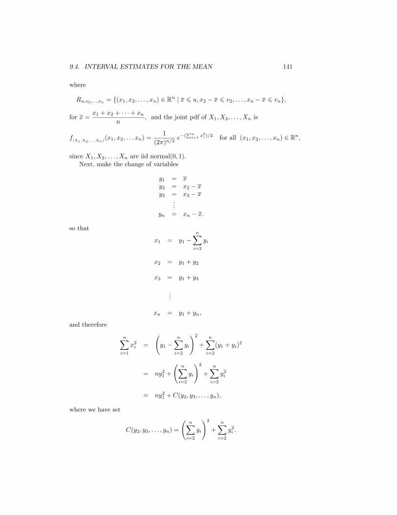
9.4. INTERVAL ESTIMATES FOR THE MEAN 141
where
Ru,v2,...,vn = {(x1, x2, . . . , xn) ∈ Rn | x 6 u, x2 − x 6 v2, . . . , xn − x 6 vn},
for x =x1 + x2 + · · ·+ xn
n, and the joint pdf of X1, X2, . . . , Xn is
f(X1,X2,...,Xn)
(x1, x2, . . . xn) =1
(2π)n/2e−(
∑ni=1 x
2i )/2 for all (x1, x2, . . . , xn) ∈ Rn,
since X1, X2, . . . , Xn are iid normal(0, 1).Next, make the change of variables
y1 = xy2 = x2 − xy3 = x3 − x
...yn = xn − x.
so that
x1 = y1 −n∑i=2
yi
x2 = y1 + y2
x3 = y1 + y3
...
xn = y1 + yn,
and therefore
n∑i=1
x2i =
(y1 −
n∑i=2
yi
)2
+
n∑i=2
(y1 + yi)2
= ny21 +
(n∑i=2
yi
)2
+
n∑i=2
y2i
= ny21 + C(y2, y3, . . . , yn),
where we have set
C(y2, y3, . . . , yn) =
(n∑i=2
yi
)2
+
n∑i=2
y2i .

142 CHAPTER 9. INTRODUCTION TO ESTIMATION
Thus, by the change of variables formula,
F(Xn,Y )
( u, v2, . . . , vn)
=
∫ u
−∞
∫ v1
−∞· · ·∫ vn
−∞
e−(ny21+C(y2,...,yn)/2
(2π)n/2
∣∣∣∣∂(x1, x2, . . . , xn)
∂(y1, y2, . . . , yn)
∣∣∣∣ dyn · · · dy1,
where
∂(x1, x2, . . . , xn)
∂(y1, y2, . . . yn)= det
1 −1 −1 · · · −11 1 0 · · · 01 0 1 · · · 0...
......
...1 0 0 · · · 1
.
In order to compute this determinant observe that
ny1 = x1 + x2 + x3 + . . . xnny2 = −x1 + (n− 1)x2 − x3 − . . .− xnny3 = −x1 − x2 + (n− 1)x3 − . . .− xn
...nyn = −x1 − x2 − x3 − . . .+ (n− 1)xn
,
which can be written in matrix form as
n
y1
y2
y3
...yn
= A
x1
x2
x3
...xn
,
where A is the n× n matrix
A =
1 1 1 · · · 1−1 (n− 1) −1 · · · −1−1 −1 (n− 1) · · · −1
......
......
−1 −1 −1 · · · (n− 1)
,
whose determinant is
detA = det
1 1 1 · · · 10 n 0 · · · 00 0 n · · · 0...
......
...0 0 0 · · · n
= nn−1.
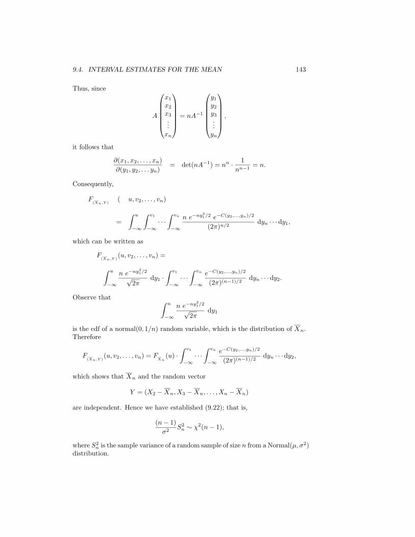
9.4. INTERVAL ESTIMATES FOR THE MEAN 143
Thus, since
A
x1
x2
x3
...xn
= nA−1
y1
y2
y3
...yn
,
it follows that
∂(x1, x2, . . . , xn)
∂(y1, y2, . . . yn)= det(nA−1) = nn · 1
nn−1= n.
Consequently,
F(Xn,Y )
( u, v2, . . . , vn)
=
∫ u
−∞
∫ v1
−∞· · ·∫ vn
−∞
n e−ny21/2 e−C(y2,...,yn)/2
(2π)n/2dyn · · · dy1,
which can be written as
F(Xn,Y )
(u, v2, . . . , vn) =
∫ u
−∞
n e−ny21/2
√2π
dy1 ·∫ v1
−∞· · ·∫ vn
−∞
e−C(y2,...,yn)/2
(2π)(n−1)/2dyn · · · dy2.
Observe that ∫ u
−∞
n e−ny21/2
√2π
dy1
is the cdf of a normal(0, 1/n) random variable, which is the distribution of Xn.Therefore
F(Xn,Y )
(u, v2, . . . , vn) = FXn
(u) ·∫ v1
−∞· · ·∫ vn
−∞
e−C(y2,...,yn)/2
(2π)(n−1)/2dyn · · · dy2,
which shows that Xn and the random vector
Y = (X2 −Xn, X3 −Xn, . . . , Xn −Xn)
are independent. Hence we have established (9.22); that is,
(n− 1)
σ2S2n ∼ χ2(n− 1),
where S2n is the sample variance of a random sample of size n from a Normal(µ, σ2)
distribution.
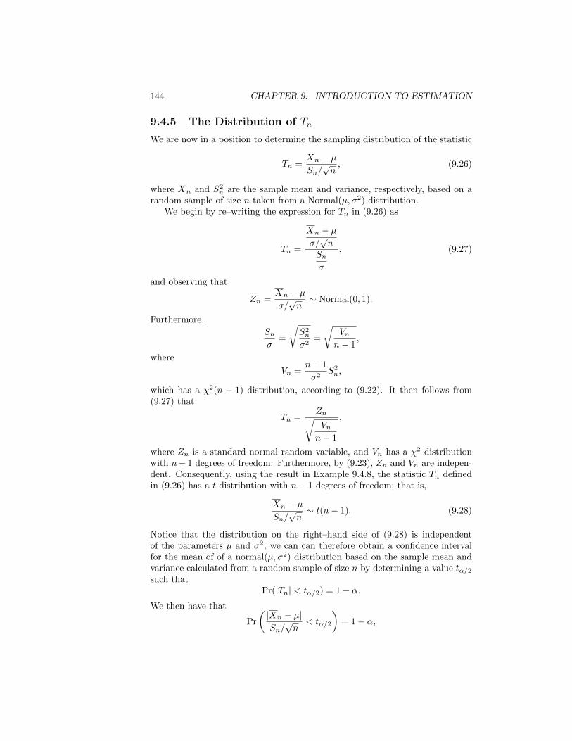
144 CHAPTER 9. INTRODUCTION TO ESTIMATION
9.4.5 The Distribution of Tn
We are now in a position to determine the sampling distribution of the statistic
Tn =Xn − µSn/√n, (9.26)
where Xn and S2n are the sample mean and variance, respectively, based on a
random sample of size n taken from a Normal(µ, σ2) distribution.We begin by re–writing the expression for Tn in (9.26) as
Tn =
Xn − µσ/√n
Snσ
, (9.27)
and observing that
Zn =Xn − µσ/√n∼ Normal(0, 1).
Furthermore,
Snσ
=
√S2n
σ2=
√Vnn− 1
,
where
Vn =n− 1
σ2S2n,
which has a χ2(n − 1) distribution, according to (9.22). It then follows from(9.27) that
Tn =Zn√Vnn− 1
,
where Zn is a standard normal random variable, and Vn has a χ2 distributionwith n− 1 degrees of freedom. Furthermore, by (9.23), Zn and Vn are indepen-dent. Consequently, using the result in Example 9.4.8, the statistic Tn definedin (9.26) has a t distribution with n− 1 degrees of freedom; that is,
Xn − µSn/√n∼ t(n− 1). (9.28)
Notice that the distribution on the right–hand side of (9.28) is independentof the parameters µ and σ2; we can can therefore obtain a confidence intervalfor the mean of of a normal(µ, σ2) distribution based on the sample mean andvariance calculated from a random sample of size n by determining a value tα/2such that
Pr(|Tn| < tα/2) = 1− α.We then have that
Pr
(|Xn − µ|Sn/√n
< tα/2
)= 1− α,
9.4. INTERVAL ESTIMATES FOR THE MEAN 145
or
Pr
(|µ−Xn| < tα/2
Sn√n
)= 1− α,
or
Pr
(Xn − tα/2
Sn√n< µ < Xn + tα/2
Sn√n
)= 1− α.
We have therefore obtained a 100(1−α)% confidence interval for the mean of anormal(µ, σ2) distribution based on the sample mean and variance of a randomsample of size n from that distribution; namely,(
Xn − tα/2Sn√n,Xn + tα/2
Sn√n
). (9.29)
To find the value for zα/2 in (9.29) we use the fact that the pdf for the tdistribution is symmetric about the vertical line at 0 (or even) to obtain that
Pr(|Tn| < t) = Pr(−t < Tn < t)
= Pr(−t < Tn 6 t)
= Pr(Tn 6 t)− Pr(Tn 6 −t)
= FTn
(t)− FTn
(−t),
where we have used the fact that Tn is a continuous random variable. Now, bythe symmetry if the pdf of Tn FTn (−t) = 1− F
Tn(t). Thus,
Pr(|Tn| < t) = 2FTn
(t)− 1 for t > 0.
So, to find tα/2 we need to solve
FTn
(t) = 1− α
2.
We therefore get that
tα/2
= F−1Tn
(1− α
2
), (9.30)
where F−1Tn
denotes the inverse of the cdf of Tn.
Example 9.4.12. Give a 95% confidence interval for the mean of a normaldistribution based on the sample mean and variance computed from a sampleof size n = 20.
Solution: In this case, α = 0.5 and Tn ∼ t(19).To find t
α/2we may use the TINV function in MS Excel, which gives the
inverse of the two–tailed cumulative distribution function of random variablewith a t distribution. That is, the inverse of the function
Pr(|Tn| > t) for t > 0.
The format for this function is

146 CHAPTER 9. INTRODUCTION TO ESTIMATION
TINV(probability,degrees_freedom)
In this case the probability of the two tails is α = 0.05 and the number ofdegrees of freedom is 19. Thus, according to (9.30), t
α/2is given by
TINV(0.05, 19) ≈ 2.09,
where we have used 0.05 because TINV in MS Excel gives two-tailed probabilitydistribution values.
We can also use WolframAlphaTM to obtain tα/2
. In WolframAlphaTM, theinverse cdf for a random variable with a t distribution is given by the functionqt whose format is
InverseCDF[tDistribution[df],probability].
Thus, WolframAlphaTM, we obtain for α = 0.05 and 19 degrees of freedom,
tα/2≈ InverseCDF[tDistribution[19], 0.975] ≈ 2.09.
Hence the 95% confidence interval for the mean, µ, of a normal(µ, σ2) distribu-tion based on the sample mean, Xn, and the sample variance, S2
n, is(Xn − 2.09
Sn√n,Xn + 2.09
Sn√n
), (9.31)
where n = 20. �


![PHY 123 EXPT Linear Momentum - Worksheetskipper.physics.sunysb.edu/~physlab/Fall2016/PHY123LinMomWorksheet.pdfPHY 123 EXPT Linear Momentum - Worksheet. ws ± Δ ws: _____[ ] m s ±](https://static.fdocument.org/doc/165x107/6048e3cef3d84b3fe3016d71/phy-123-expt-linear-momentum-physlabfall2016phy123linmomworksheetpdf-phy-123.jpg)