Probabilistic Inference Lecture 3 M. Pawan Kumar [email protected] Slides available online
122
Probabilistic Inference Lecture 3 M. Pawan Kumar [email protected] es available online http://cvc.centrale-ponts.fr/personnel/pa
-
Upload
crystal-logan -
Category
Documents
-
view
219 -
download
3
Transcript of Probabilistic Inference Lecture 3 M. Pawan Kumar [email protected] Slides available online
Probabilistic InferenceLecture 3
M. Pawan Kumar
Slides available online http://cvc.centrale-ponts.fr/personnel/pawan/

Recap of lecture 1
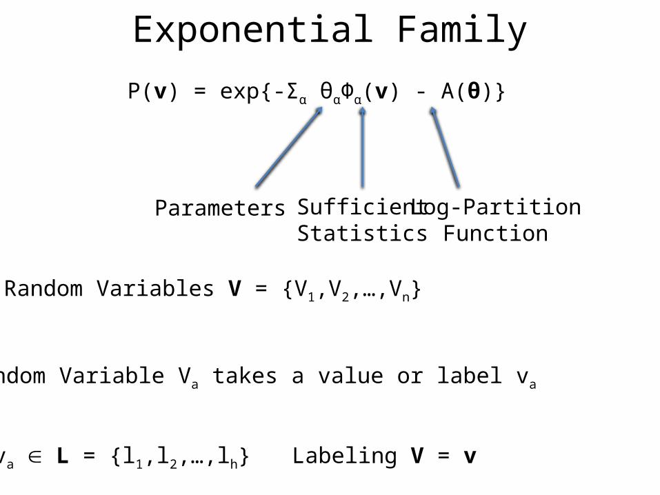
Exponential Family
P(v) = exp{-Σα θαΦα(v) - A(θ)}
SufficientStatistics
Parameters Log-PartitionFunction
Random Variables V = {V1,V2,…,Vn}
Labeling V = vva L = {l1,l2,…,lh}
Random Variable Va takes a value or label va
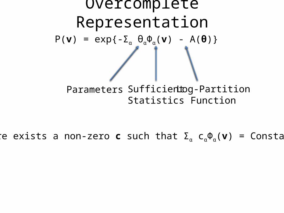
Overcomplete Representation
P(v) = exp{-Σα θαΦα(v) - A(θ)}
SufficientStatistics
Parameters Log-PartitionFunction
There exists a non-zero c such that Σα cαΦα(v) = Constant

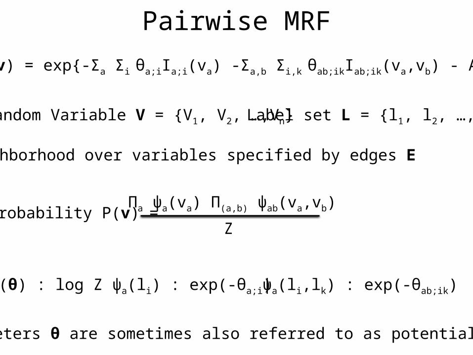
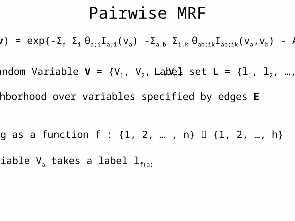
Pairwise MRF
Random Variable V = {V1, V2, …,Vn}
Neighborhood over variables specified by edges E
Label set L = {l1, l2, …, lh}
P(v) = exp{-Σα θαΦα(v) - A(θ)}
Sufficient Statistics Parameters
Ia;i(va) θa;ifor all Va V, li L
θab;ik for all (Va,Vb) E, li, lk L
Iab;ik(va,vb)
Pairwise MRF
Random Variable V = {V1, V2, …,Vn}
Neighborhood over variables specified by edges E
Label set L = {l1, l2, …, lh}
P(v) = exp{-Σa Σi θa;iIa;i(va) -Σa,b Σi,k θab;ikIab;ik(va,vb) - A(θ)}
A(θ) : log Z
Probability P(v) =Πa ψa(va) Π(a,b) ψab(va,vb)
Z
ψa(li) : exp(-θa;i) ψa(li,lk) : exp(-θab;ik)
Parameters θ are sometimes also referred to as potentials
Pairwise MRF
Random Variable V = {V1, V2, …,Vn}
Neighborhood over variables specified by edges E
Label set L = {l1, l2, …, lh}
P(v) = exp{-Σa Σi θa;iIa;i(va) -Σa,b Σi,k θab;ikIab;ik(va,vb) - A(θ)}
Labeling as a function f : {1, 2, … , n} {1, 2, …, h}
Variable Va takes a label lf(a)
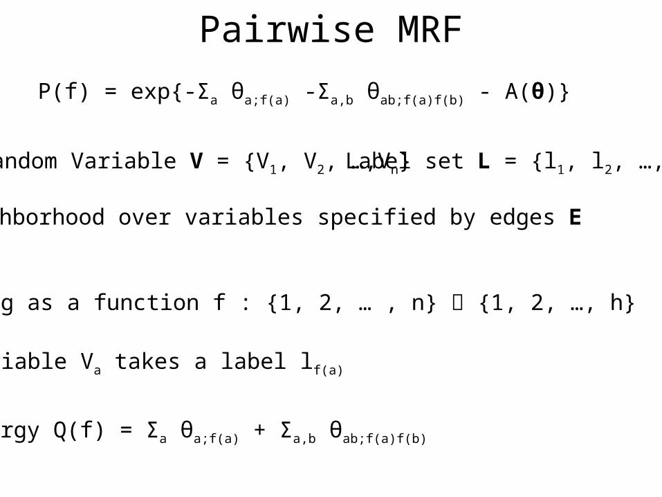
Pairwise MRF
Random Variable V = {V1, V2, …,Vn}
Neighborhood over variables specified by edges E
Label set L = {l1, l2, …, lh}
P(f) = exp{-Σa θa;f(a) -Σa,b θab;f(a)f(b) - A(θ)}
Labeling as a function f : {1, 2, … , n} {1, 2, …, h}
Variable Va takes a label lf(a)
Energy Q(f) = Σa θa;f(a) + Σa,b θab;f(a)f(b)

Pairwise MRF
Random Variable V = {V1, V2, …,Vn}
Neighborhood over variables specified by edges E
Label set L = {l1, l2, …, lh}
P(f) = exp{-Q(f) - A(θ)}
Labeling as a function f : {1, 2, … , n} {1, 2, …, h}
Variable Va takes a label lf(a)
Energy Q(f) = Σa θa;f(a) + Σa,b θab;f(a)f(b)
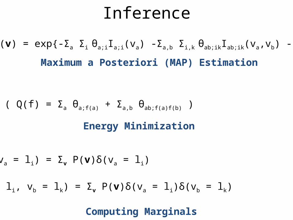
Inference
maxv ( P(v) = exp{-Σa Σi θa;iIa;i(va) -Σa,b Σi,k θab;ikIab;ik(va,vb) - A(θ)} )
Maximum a Posteriori (MAP) Estimation
minf ( Q(f) = Σa θa;f(a) + Σa,b θab;f(a)f(b) )
Energy Minimization
P(va = li) = Σv P(v)δ(va = li)
Computing Marginals
P(va = li, vb = lk) = Σv P(v)δ(va = li)δ(vb = lk)
Recap of lecture 2
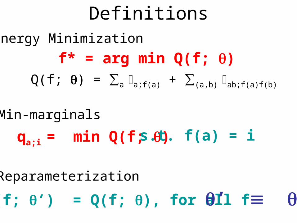
DefinitionsEnergy Minimization
f* = arg min Q(f; )Q(f; ) = ∑a a;f(a) + ∑(a,b) ab;f(a)f(b)
Min-marginals
qa;i = min Q(f; ) s.t. f(a) = i
Q(f; ’) = Q(f; ), for all f ’ Reparameterization

Belief PropagationPearl, 1988
General form of Reparameterization
’a;i = a;i
’ab;ik = ab;ik
+ Mab;k
- Mab;k
+ Mba;i
- Mba;i
’b;k = b;k
Reparameterization of (a,b) in Belief Propagation
Mab;k = mini { a;i + ab;ik }
Mba;i = 0
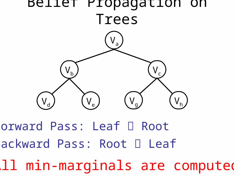
Belief Propagation on Trees
Vb
Va
Forward Pass: Leaf Root
All min-marginals are computed
Backward Pass: Root Leaf
Vc
Vd Ve Vg Vh
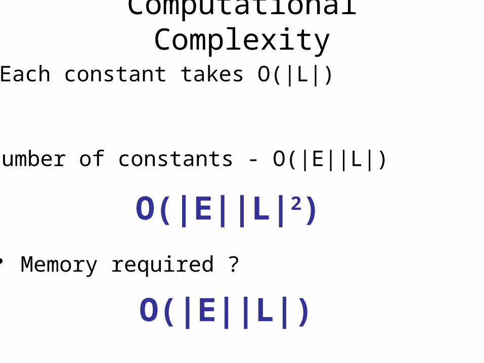
Computational Complexity
• Each constant takes O(|L|)
• Number of constants - O(|E||L|)
O(|E||L|2)
• Memory required ?
O(|E||L|)
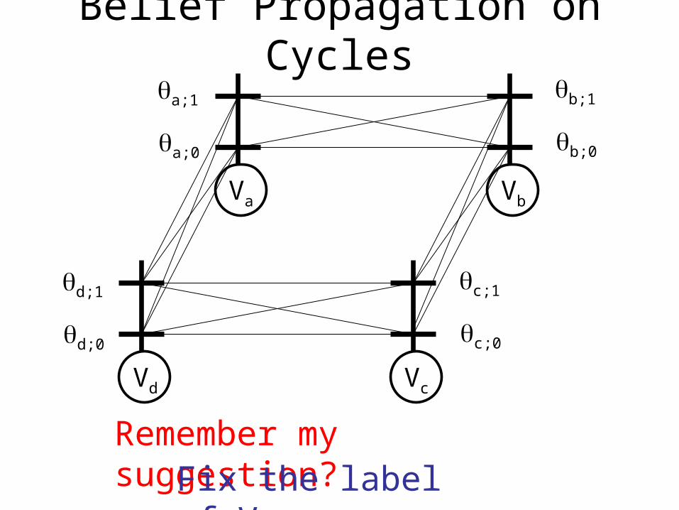
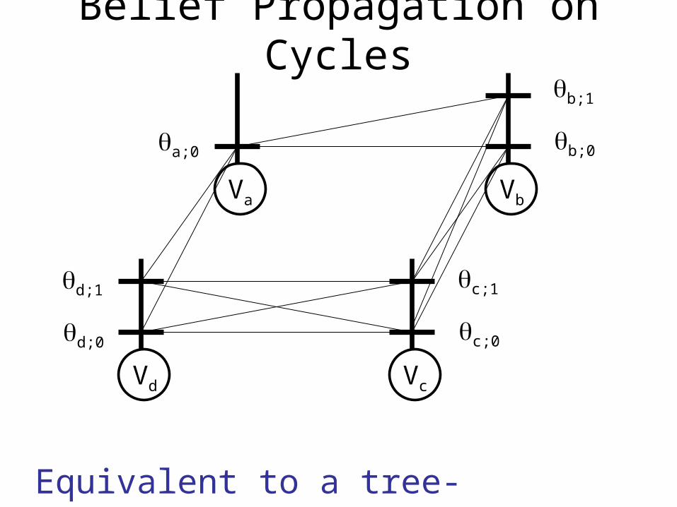
Belief Propagation on Cycles
Va Vb
Vd Vc
a;0
a;1
b;0
b;1
d;0
d;1
c;0
c;1
Remember my suggestion?Fix the label of Va
Belief Propagation on Cycles
Va Vb
Vd Vc
a;0 b;0
b;1
d;0
d;1
c;0
c;1
Equivalent to a tree-structured problem

Belief Propagation on Cycles
Va Vb
Vd Vc
a;1
b;0
b;1
d;0
d;1
c;0
c;1
Equivalent to a tree-structured problem

Belief Propagation on Cycles
Choose the minimum energy solution
Va Vb
Vd Vc
a;0
a;1
b;0
b;1
d;0
d;1
c;0
c;1
This approach quickly becomes infeasible

Vincent Algayres Algorithm
Va Vb
Vd Vc
a;0 b;0
d;0
d;1
c;0
c;1
Compute zero cost paths from all labels of Va to all labels of Vd. Requires fixing Va.
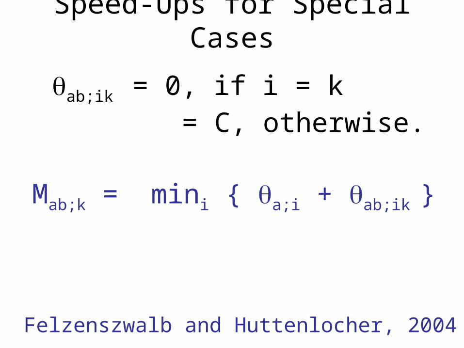
Speed-Ups for Special Cases
ab;ik = 0, if i = k
= C, otherwise.
Mab;k = mini { a;i + ab;ik }
Felzenszwalb and Huttenlocher, 2004
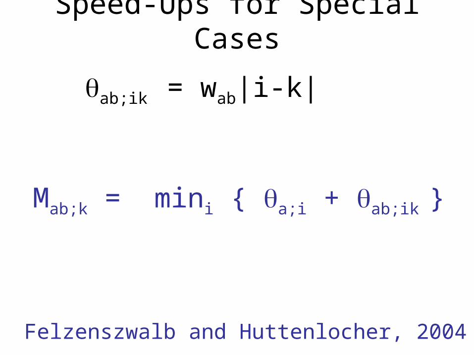
Speed-Ups for Special Cases
ab;ik = wab|i-k|
Mab;k = mini { a;i + ab;ik }
Felzenszwalb and Huttenlocher, 2004
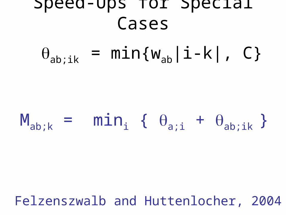
Speed-Ups for Special Cases
ab;ik = min{wab|i-k|, C}
Mab;k = mini { a;i + ab;ik }
Felzenszwalb and Huttenlocher, 2004

Speed-Ups for Special Cases
ab;ik = min{wab(i-k)2, C}
Mab;k = mini { a;i + ab;ik }
Felzenszwalb and Huttenlocher, 2004

Lecture 3
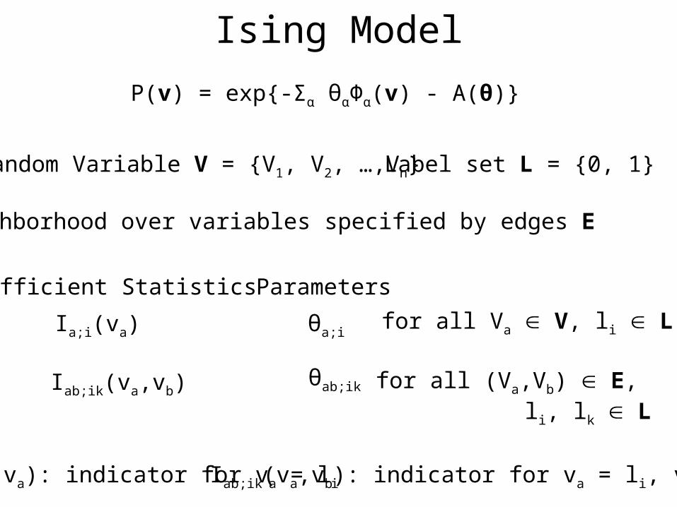
Ising Model
P(v) = exp{-Σα θαΦα(v) - A(θ)}
Random Variable V = {V1, V2, …,Vn} Label set L = {0, 1}
Neighborhood over variables specified by edges E
Sufficient Statistics Parameters
Ia;i(va) θa;ifor all Va V, li L
θab;ik for all (Va,Vb) E, li, lk L
Iab;ik(va,vb)
Ia;i(va): indicator for va = li Iab;ik(va,vb): indicator for va = li, vb = lk
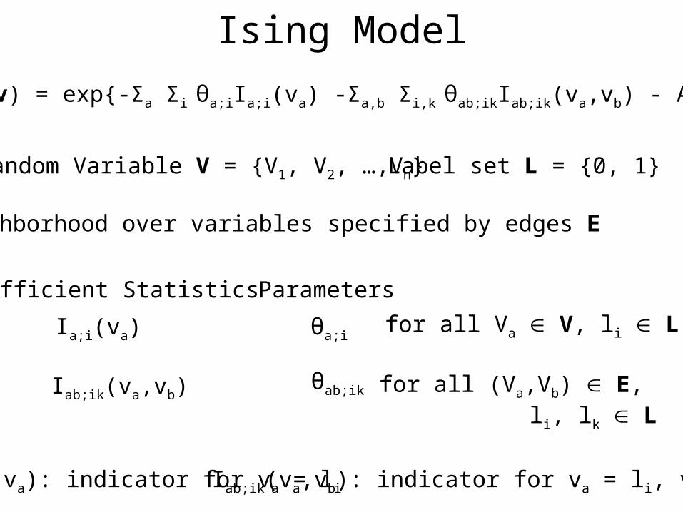
Ising Model
P(v) = exp{-Σa Σi θa;iIa;i(va) -Σa,b Σi,k θab;ikIab;ik(va,vb) - A(θ)}
Random Variable V = {V1, V2, …,Vn} Label set L = {0, 1}
Neighborhood over variables specified by edges E
Sufficient Statistics Parameters
Ia;i(va) θa;ifor all Va V, li L
θab;ik for all (Va,Vb) E, li, lk L
Iab;ik(va,vb)
Ia;i(va): indicator for va = li Iab;ik(va,vb): indicator for va = li, vb = lk
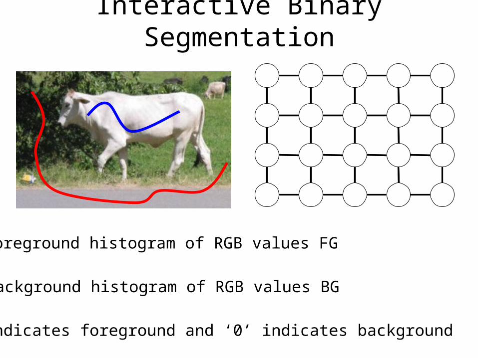
Interactive Binary Segmentation
Foreground histogram of RGB values FG
Background histogram of RGB values BG
‘1’ indicates foreground and ‘0’ indicates background

Interactive Binary Segmentation
More likely to be foreground than background

Interactive Binary Segmentation
More likely to be background than foreground
θa;0 proportional to -log(BG(da))
θa;1 proportional to -log(FG(da))
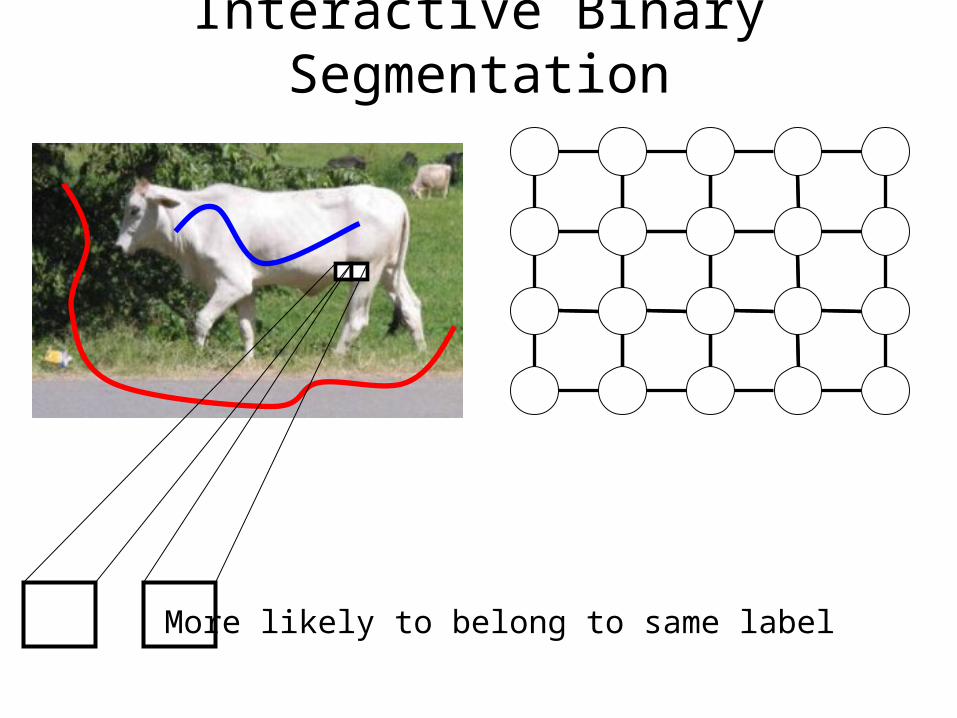
Interactive Binary Segmentation
More likely to belong to same label
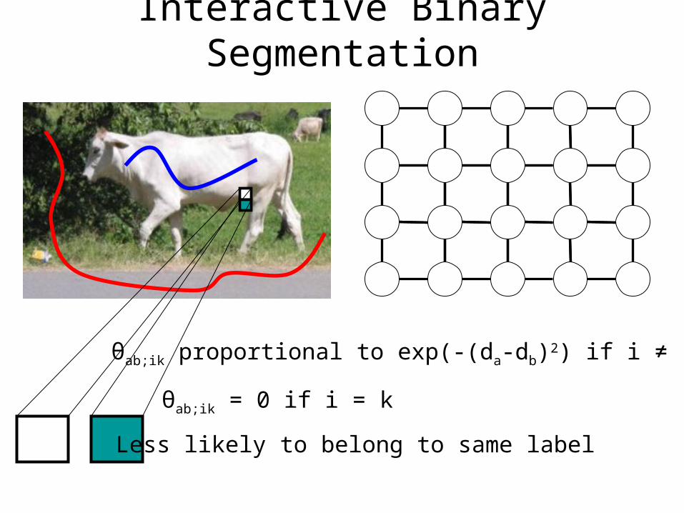
Interactive Binary Segmentation
Less likely to belong to same label
θab;ik proportional to exp(-(da-db)2) if i ≠ k
θab;ik = 0 if i = k
Outline
• Minimum Cut Problem
• Two-Label Submodular Energy Functions
• Move-Making Algorithms
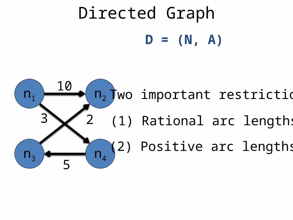
Directed Graph
n1 n2
n3 n4
10
5
3 2
Two important restrictions
(1) Rational arc lengths
(2) Positive arc lengths
D = (N, A)

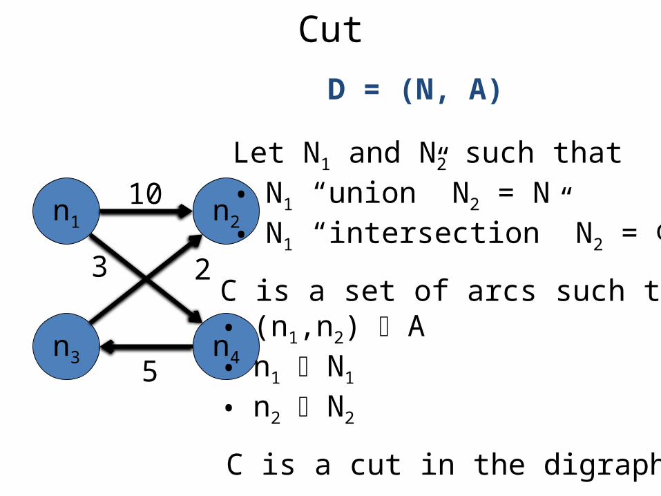
Cut
n1 n2
n3 n4
10
5
3 2
Let N1 and N2 such that
• N1 “union” N2 = N
• N1 “intersection” N2 = Φ
C is a set of arcs such that• (n1,n2) A• n1 N1
• n2 N2
D = (N, A)
C is a cut in the digraph D
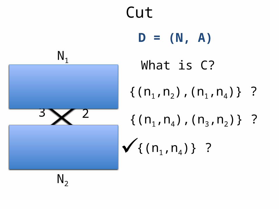
Cut
n1 n2
n3 n4
10
5
3 2
What is C?
D = (N, A)
N1
N2
{(n1,n2),(n1,n4)} ?
{(n1,n4),(n3,n2)} ?
{(n1,n4)} ?✓
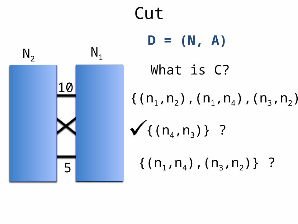
Cut
n1 n2
n3 n4
10
5
3 2
What is C?
D = (N, A)N1N2
{(n1,n2),(n1,n4),(n3,n2)} ?
{(n1,n4),(n3,n2)} ?
{(n4,n3)} ?✓

Cut
n1 n2
n3 n4
10
5
3 2
What is C?
D = (N, A)N2N1
{(n1,n2),(n1,n4),(n3,n2)} ?
{(n1,n4),(n3,n2)} ?
{(n3,n2)} ?
✓
Cut
n1 n2
n3 n4
10
5
3 2
Let N1 and N2 such that
• N1 “union” N2 = N
• N1 “intersection” N2 = Φ
C is a set of arcs such that• (n1,n2) A• n1 N1
• n2 N2
D = (N, A)
C is a cut in the digraph D

Weight of a Cut
n1 n2
n3 n4
10
5
3 2 Sum of length of allarcs in C
D = (N, A)

Weight of a Cut
n1 n2
n3 n4
10
5
3 2 w(C) = Σ(n1,n2) C l(n1,n2)
D = (N, A)
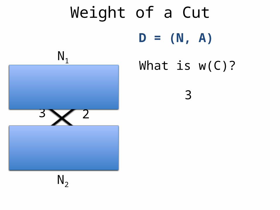
Weight of a Cut
n1 n2
n3 n4
10
5
3 2
What is w(C)?
D = (N, A)
N1
N2
3
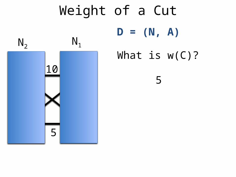
Weight of a Cut
n1 n2
n3 n4
10
5
3 2
What is w(C)?
D = (N, A)N1N2
5

Weight of a Cut
n1 n2
n3 n4
10
5
3 2
What is w(C)?
D = (N, A)N2N1
15
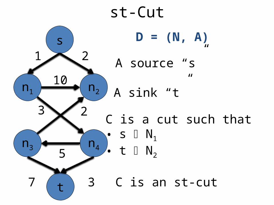
st-Cut
n1 n2
n3 n4
10
5
3 2
A source “s”
C is a cut such that• s N1
• t N2
D = (N, A)
C is an st-cut
s
t
A sink “t”
1 2
7 3
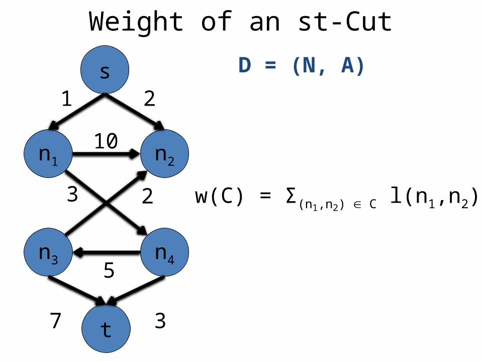
Weight of an st-Cut
n1 n2
n3 n4
10
5
3 2
D = (N, A)s
t
1 2
7 3
w(C) = Σ(n1,n2) C l(n1,n2)
Weight of an st-Cut
n1 n2
n3 n4
10
5
3 2
D = (N, A)s
t
1 2
7 3
What is w(C)?
3
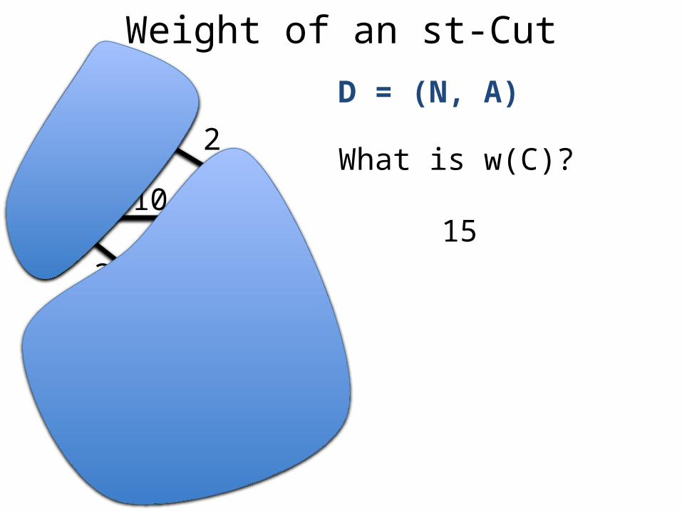
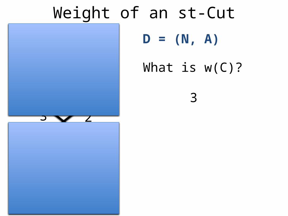
Weight of an st-Cut
n1 n2
n3 n4
10
5
3 2
D = (N, A)s
t
1 2
7 3
What is w(C)?
15
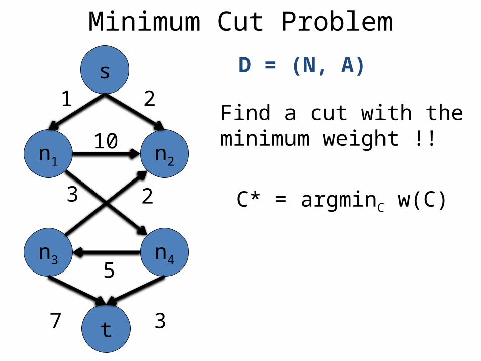
Minimum Cut Problem
n1 n2
n3 n4
10
5
3 2
D = (N, A)s
t
1 2
7 3
Find a cut with theminimum weight !!
C* = argminC w(C)
[Slide credit: Andrew Goldberg]
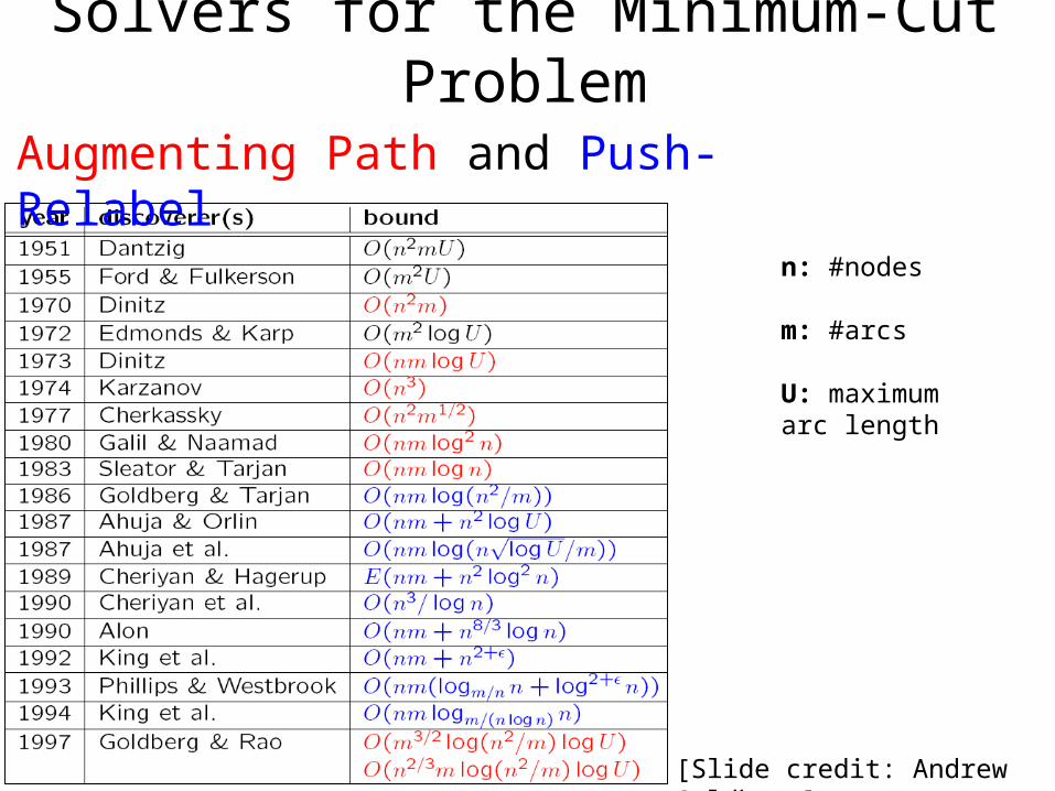
Augmenting Path and Push-Relabel
n: #nodes
m: #arcs
U: maximumarc length
Solvers for the Minimum-Cut Problem

Remember …
Two important restrictions
(1) Rational arc lengths
(2) Positive arc lengths

Cut
n1 n2
n3 n4
10
5
3 2
Let N1 and N2 such that
• N1 “union” N2 = N
• N1 “intersection” N2 = Φ
C is a set of arcs such that• (n1,n2) A• n1 N1
• n2 N2
D = (N, A)
C is a cut in the digraph D

st-Cut
n1 n2
n3 n4
10
5
3 2
A source “s”
C is a cut such that• s N1
• t N2
D = (N, A)
C is an st-cut
s
t
A sink “t”
1 2
7 3

Minimum Cut Problem
n1 n2
n3 n4
10
5
3 2
D = (N, A)s
t
1 2
7 3
Find a cut with theminimum weight !!
C* = argminC w(C)
w(C) = Σ(n1,n2) C l(n1,n2)

Outline
• Minimum Cut Problem
• Two-Label Submodular Energy Functions
• Move-Making Algorithms
Hammer, 1965; Kolmogorov and Zabih, 2004
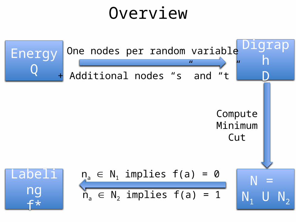
Overview
Energy Q
DigraphD
One nodes per random variable
N = N1 U N2
ComputeMinimum
Cut
+ Additional nodes “s” and “t”
Labelingf*
na N1 implies f(a) = 0
na N2 implies f(a) = 1
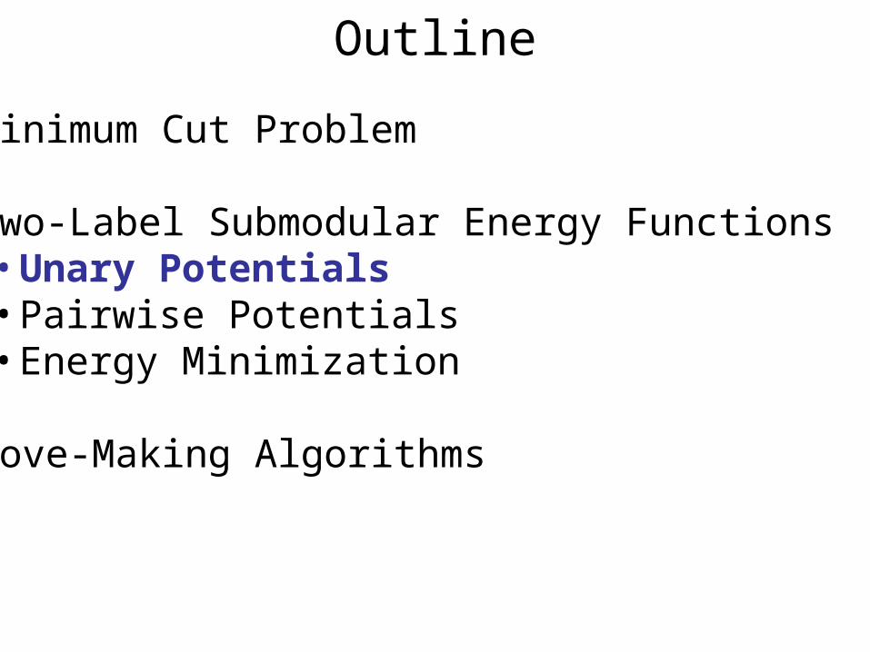
Outline
• Minimum Cut Problem
• Two-Label Submodular Energy Functions• Unary Potentials• Pairwise Potentials• Energy Minimization
• Move-Making Algorithms

Digraph for Unary Potentials
Va
θa;0
θa;1P
Q
f(a) = 0
f(a) = 1
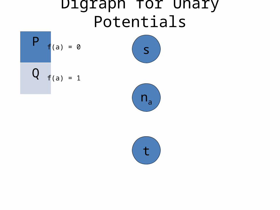
Digraph for Unary Potentials
na
P
Q
s
t
f(a) = 0
f(a) = 1

Digraph for Unary Potentials
na
P
Q
s
t
Let P ≥ Q
P-Q
0
Q
Q+
ConstantP-Q
f(a) = 0
f(a) = 1
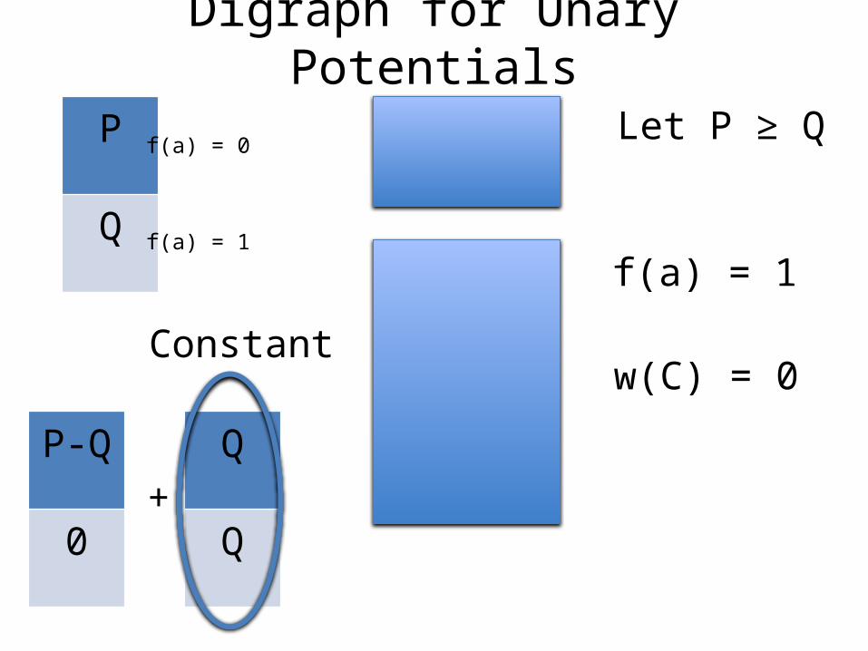
Digraph for Unary Potentials
na
P
Q
s
t
Let P ≥ Q
P-Q
0
Q
Q+
ConstantP-Q
f(a) = 1
w(C) = 0
f(a) = 0
f(a) = 1
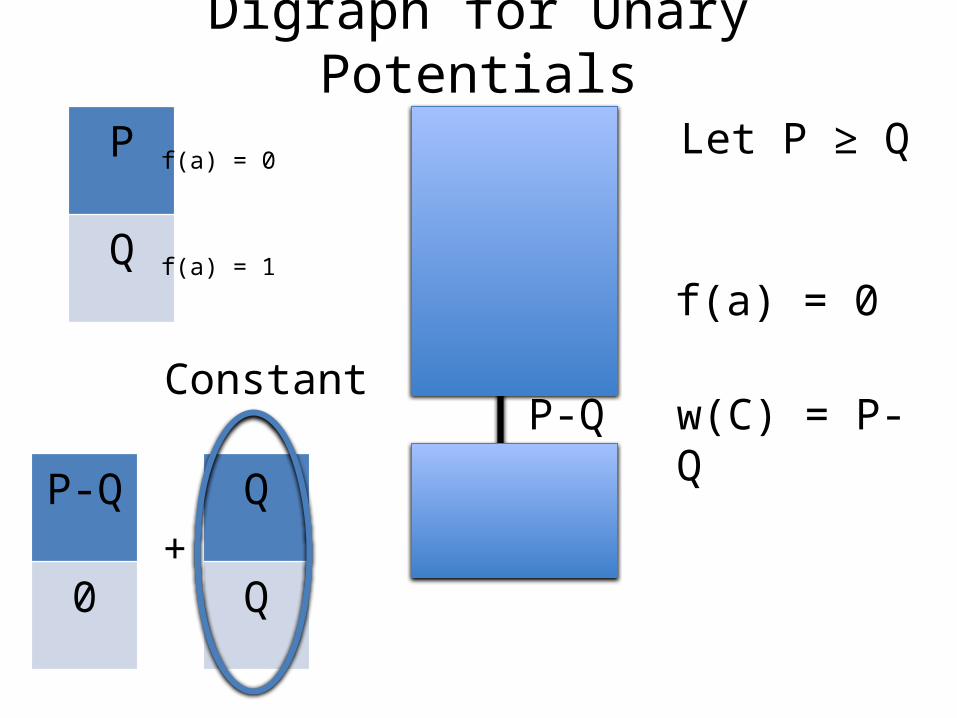
Digraph for Unary Potentials
na
P
Q
s
t
Let P ≥ Q
P-Q
0
Q
Q+
ConstantP-Q
f(a) = 0
w(C) = P-Q
f(a) = 0
f(a) = 1
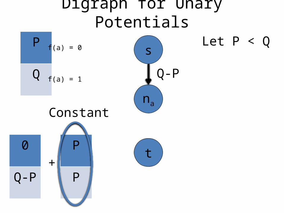
Digraph for Unary Potentials
na
P
Q
s
t
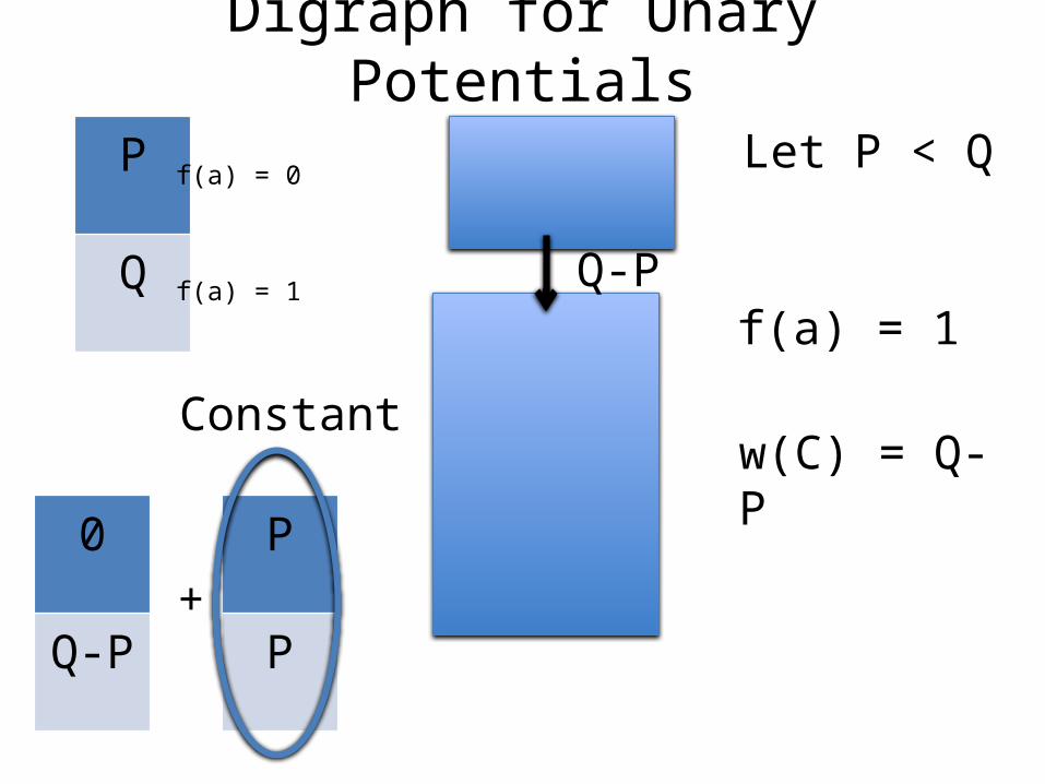
Let P < Q
0
Q-P
P
P+
Constant
Q-P
f(a) = 0
f(a) = 1
Digraph for Unary Potentials
na
P
Q
s
t
Let P < Q
0
Q-P
P
P+
Constant
f(a) = 1
w(C) = Q-P
Q-P
f(a) = 0
f(a) = 1

Digraph for Unary Potentials
na
P
Q
s
t
Let P < Q
0
Q-P
P
P+
Constant
f(a) = 0
w(C) = 0
Q-P
f(a) = 0
f(a) = 1
Outline
• Minimum Cut Problem
• Two-Label Submodular Energy Functions• Unary Potentials• Pairwise Potentials• Energy Minimization
• Move-Making Algorithms
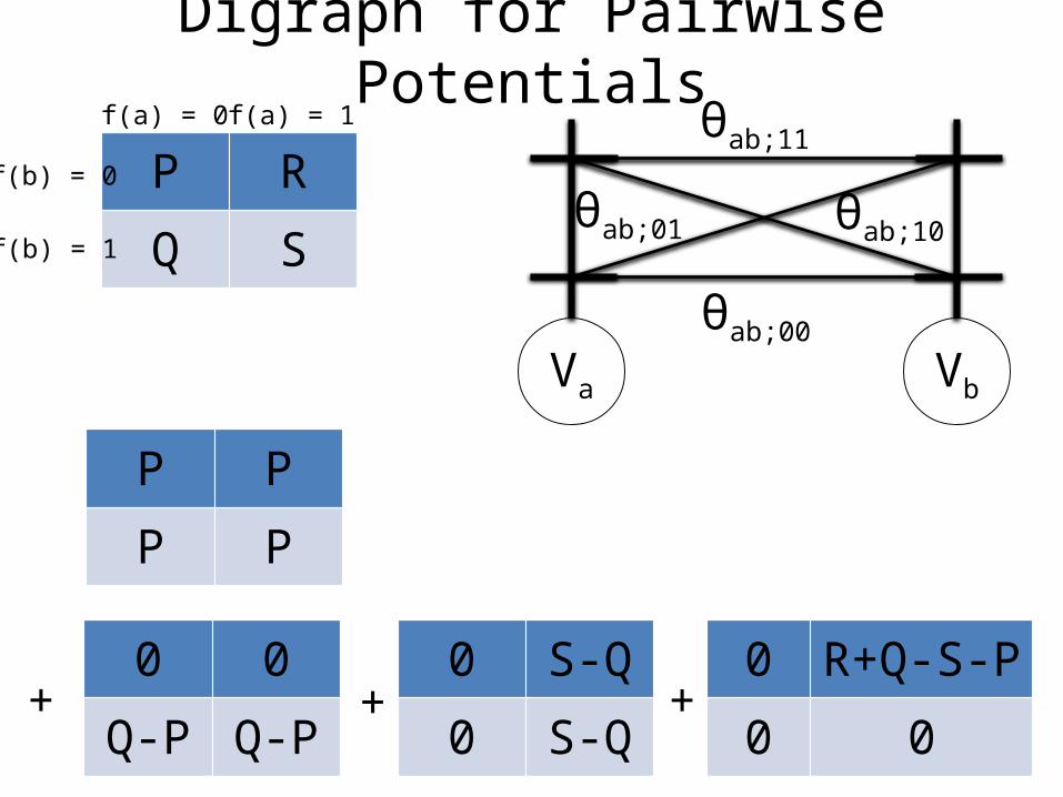
Digraph for Pairwise Potentials
Va
θab;11
Vb
θab;00
θab;01 θab;10
P R
Q S
f(a) = 0 f(a) = 1
f(b) = 0
f(b) = 1
0 0
Q-P Q-P
0 S-Q
0 S-Q
0 R+Q-S-P
0 0+ + +
P P
P P
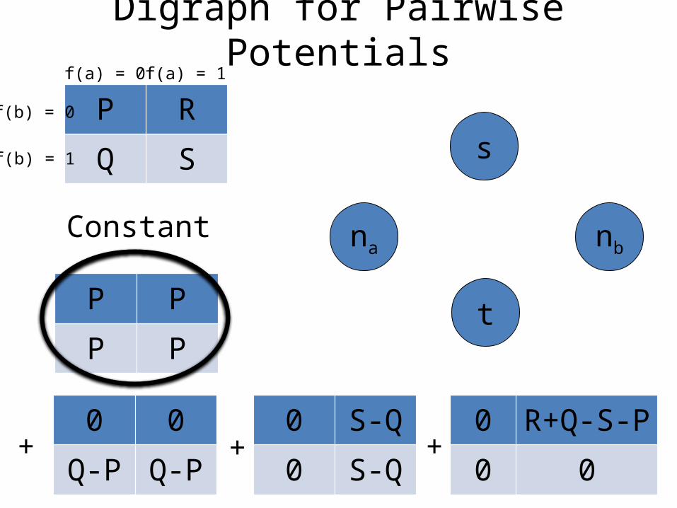
Digraph for Pairwise Potentials
na nb
P R
Q S
f(a) = 0 f(a) = 1
f(b) = 0
f(b) = 1
0 0
Q-P Q-P
0 S-Q
0 S-Q
0 R+Q-S-P
0 0+ + +
P P
P P
s
t
Constant
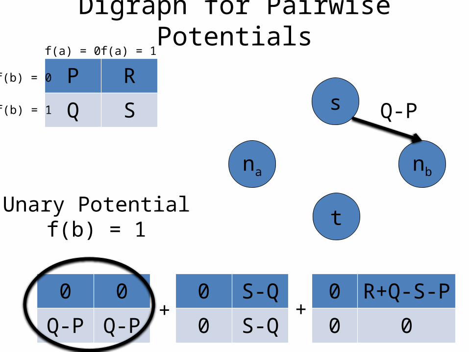
Digraph for Pairwise Potentials
na nb
P R
Q S
0 0
Q-P Q-P
0 S-Q
0 S-Q
0 R+Q-S-P
0 0+ +
s
tUnary Potential
f(b) = 1
Q-P
f(a) = 0 f(a) = 1
f(b) = 0
f(b) = 1
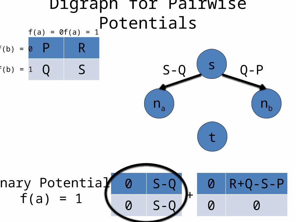
Digraph for Pairwise Potentials
na nb
P R
Q S
0 S-Q
0 S-Q
0 R+Q-S-P
0 0+
s
t
Unary Potentialf(a) = 1
Q-PS-Q
f(a) = 0 f(a) = 1
f(b) = 0
f(b) = 1

Digraph for Pairwise Potentials
na nb
P R
Q S
0 R+Q-S-P
0 0
s
t
Pairwise Potentialf(a) = 1, f(b) = 0
Q-PS-Q
f(a) = 0 f(a) = 1
f(b) = 0
f(b) = 1
R+Q-S-P
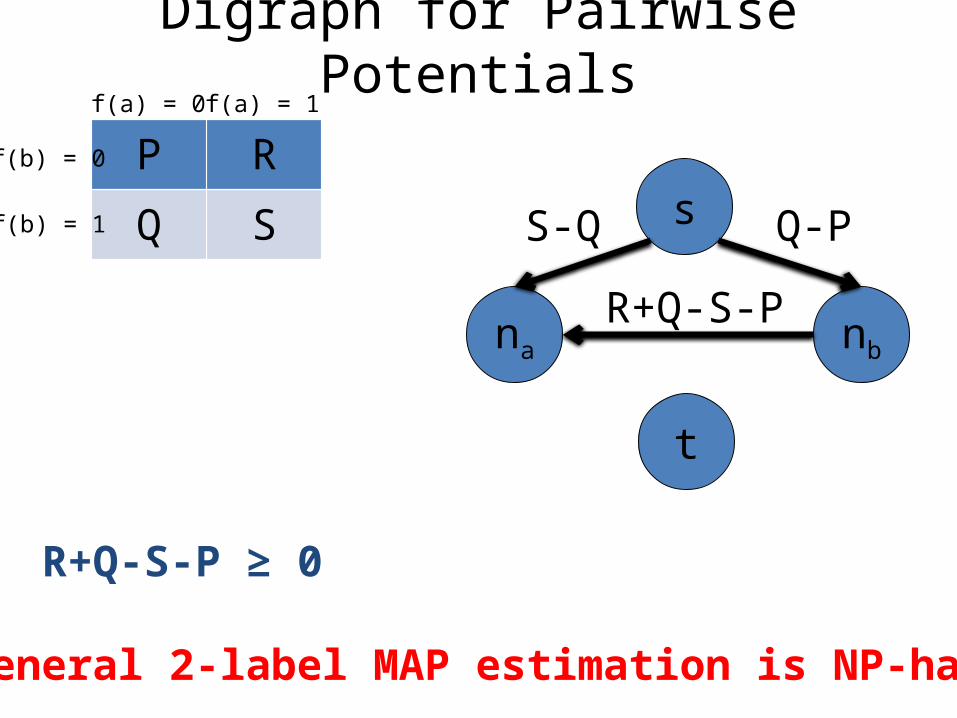
Digraph for Pairwise Potentials
na nb
P R
Q S s
t
Q-PS-Q
f(a) = 0 f(a) = 1
f(b) = 0
f(b) = 1
R+Q-S-P
R+Q-S-P ≥ 0
General 2-label MAP estimation is NP-hard
Outline
• Minimum Cut Problem
• Two-Label Submodular Energy Functions• Unary Potentials• Pairwise Potentials• Energy Minimization
• Move-Making Algorithms

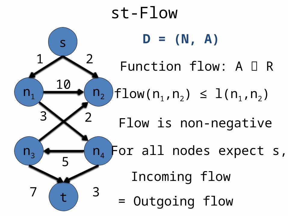
st-Flow
n1 n2
n3 n4
10
5
3 2
D = (N, A)s
t
1 2
7 3
Function flow: A R
Flow is less than length
Flow is non-negative
For all nodes expect s,t
Incoming flow
= Outgoing flow
st-Flow
n1 n2
n3 n4
10
5
3 2
D = (N, A)s
t
1 2
7 3
Function flow: A R
Flow is non-negative
For all nodes expect s,t
Incoming flow
= Outgoing flow
flow(n1,n2) ≤ l(n1,n2)

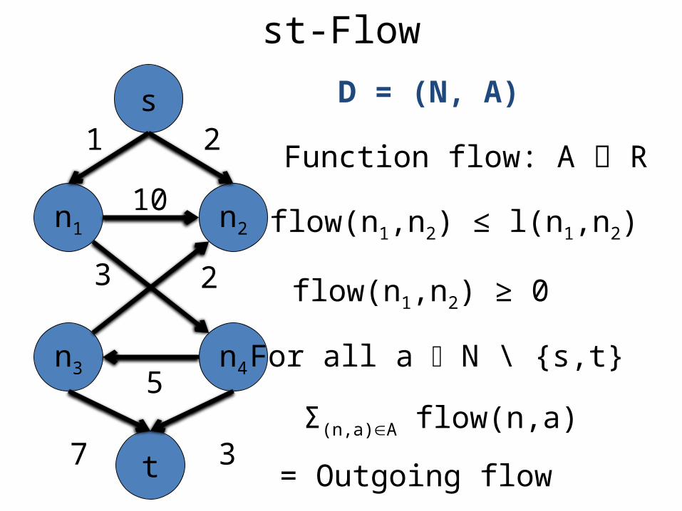
st-Flow
n1 n2
n3 n4
10
5
3 2
D = (N, A)s
t
1 2
7 3
Function flow: A R
For all nodes expect s,t
Incoming flow
= Outgoing flow
flow(n1,n2) ≥ 0
flow(n1,n2) ≤ l(n1,n2)

st-Flow
n1 n2
n3 n4
10
5
3 2
D = (N, A)s
t
1 2
7 3
Function flow: A R
Incoming flow
= Outgoing flow
For all a N \ {s,t}
flow(n1,n2) ≥ 0
flow(n1,n2) ≤ l(n1,n2)
st-Flow
n1 n2
n3 n4
10
5
3 2
D = (N, A)s
t
1 2
7 3
Function flow: A R
= Outgoing flow
For all a N \ {s,t}
Σ(n,a)A flow(n,a)
flow(n1,n2) ≥ 0
flow(n1,n2) ≤ l(n1,n2)
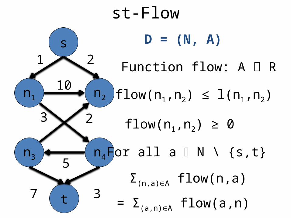
st-Flow
n1 n2
n3 n4
10
5
3 2
D = (N, A)s
t
1 2
7 3
Function flow: A R
For all a N \ {s,t}
Σ(n,a)A flow(n,a)
= Σ(a,n)A flow(a,n)
flow(n1,n2) ≥ 0
flow(n1,n2) ≤ l(n1,n2)
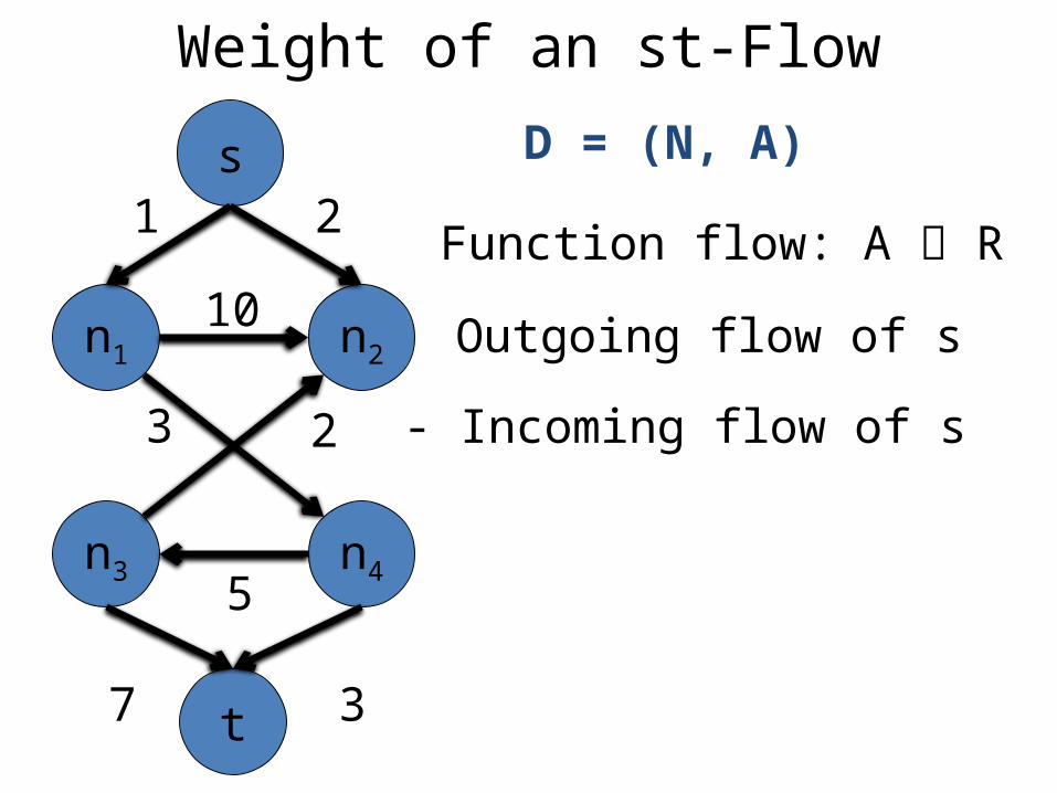
Weight of an st-Flow
n1 n2
n3 n4
10
5
3 2
D = (N, A)s
t
1 2
7 3
Function flow: A R
Outgoing flow of s
- Incoming flow of s
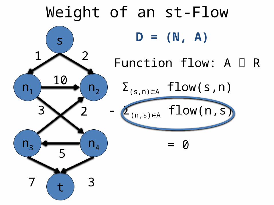
Weight of an st-Flow
n1 n2
n3 n4
10
5
3 2
D = (N, A)s
t
1 2
7 3
Function flow: A R
Σ(s,n)A flow(s,n)
- Σ(n,s)A flow(n,s)
= 0

Weight of an st-Flow
n1 n2
n3 n4
10
5
3 2
D = (N, A)s
t
1 2
7 3
Function flow: A R
Σ(s,n)A flow(s,n)
Weight of an st-Flow
n1 n2
n3 n4
10
5
3 2
D = (N, A)s
t
1 2
7 3
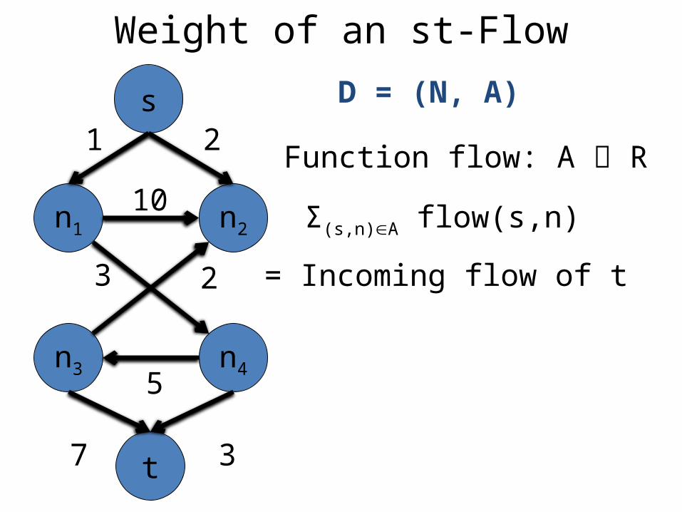
Function flow: A R
Σ(s,n)A flow(s,n)
= Incoming flow of t

Weight of an st-Flow
n1 n2
n3 n4
10
5
3 2
D = (N, A)s
t
1 2
7 3
Function flow: A R
Σ(s,n)A flow(s,n)
= Σ(n,t)A flow(n,t)
Max-Flow Problem
n1 n2
n3 n4
10
5
3 2
D = (N, A)s
t
1 2
7 3
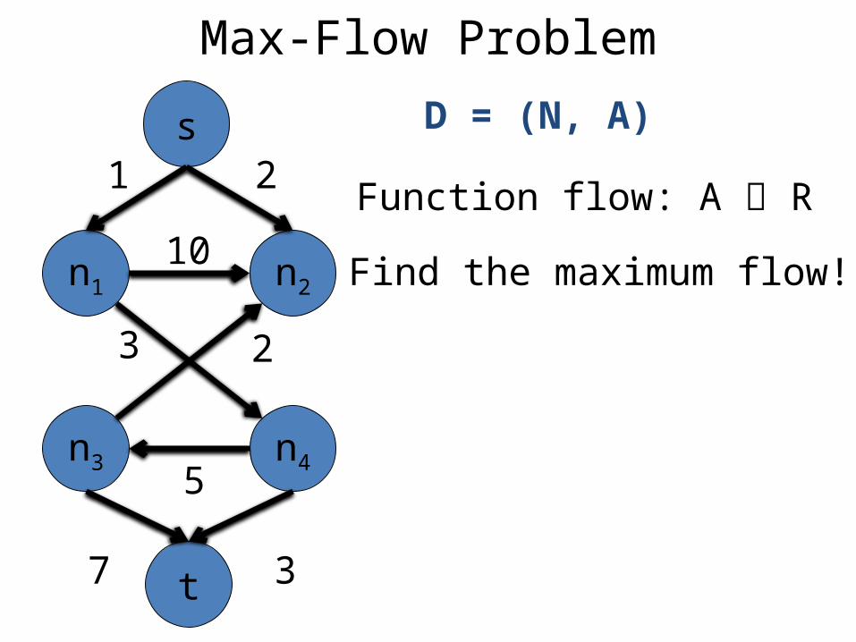
Function flow: A R
Find the maximum flow!!
Min-Cut Max-Flow Theorem
n1 n2
n3 n4
10
5
3 2
D = (N, A)s
t
1 2
7 3
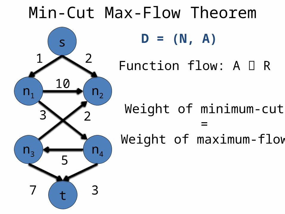
Function flow: A R
Weight of minimum-cut=
Weight of maximum-flow
Max-Flow via Reparameterization !!

Following slides courtesyPushmeet Kohli
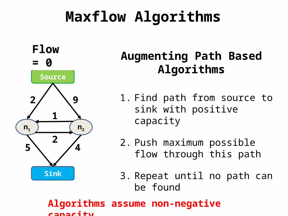
Maxflow Algorithms
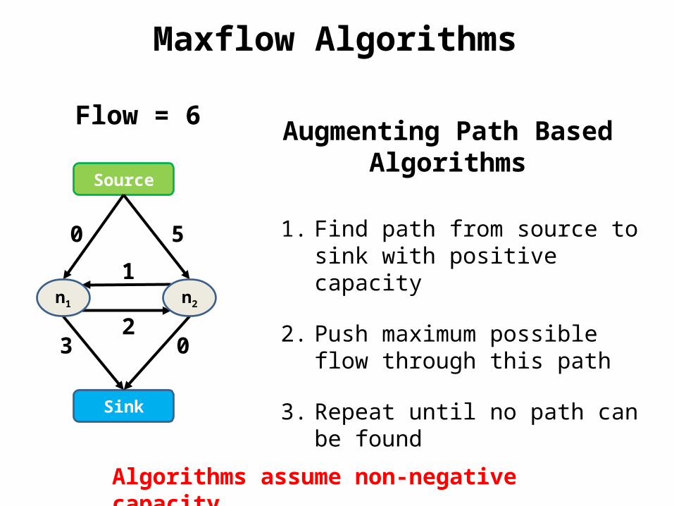
Augmenting Path Based Algorithms
1. Find path from source to sink with positive capacity
2. Push maximum possible flow through this path
3. Repeat until no path can be found
Source
Sink
n1 n2
2
5
9
42
1
Algorithms assume non-negative capacity
Flow = 0

Maxflow Algorithms
Augmenting Path Based Algorithms
1. Find path from source to sink with positive capacity
2. Push maximum possible flow through this path
3. Repeat until no path can be found
Source
Sink
n1 n2
2
5
9
42
1
Algorithms assume non-negative capacity
Flow = 0
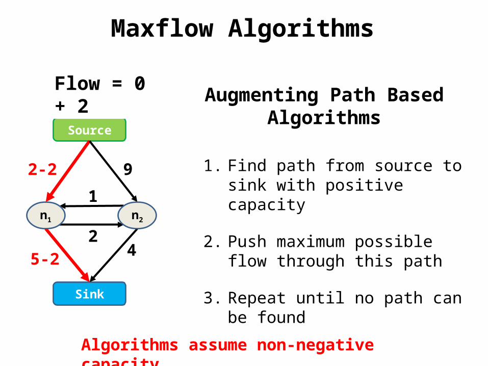
Maxflow Algorithms
Augmenting Path Based Algorithms
1. Find path from source to sink with positive capacity
2. Push maximum possible flow through this path
3. Repeat until no path can be found
Source
Sink
2-2
5-2
9
42
1
Algorithms assume non-negative capacity
Flow = 0 + 2
n1 n2

Maxflow Algorithms
Source
Sink
0
3
9
42
1
Augmenting Path Based Algorithms
1. Find path from source to sink with positive capacity
2. Push maximum possible flow through this path
3. Repeat until no path can be found
Algorithms assume non-negative capacity
Flow = 2
n1 n2

Maxflow Algorithms
Source
Sink
0
3
9
42
1
Augmenting Path Based Algorithms
1. Find path from source to sink with positive capacity
2. Push maximum possible flow through this path
3. Repeat until no path can be found
Algorithms assume non-negative capacity
Flow = 2
n1 n2

Maxflow Algorithms
Source
Sink
0
3
9
42
1
Augmenting Path Based Algorithms
1. Find path from source to sink with positive capacity
2. Push maximum possible flow through this path
3. Repeat until no path can be found
Algorithms assume non-negative capacity
Flow = 2
n1 n2
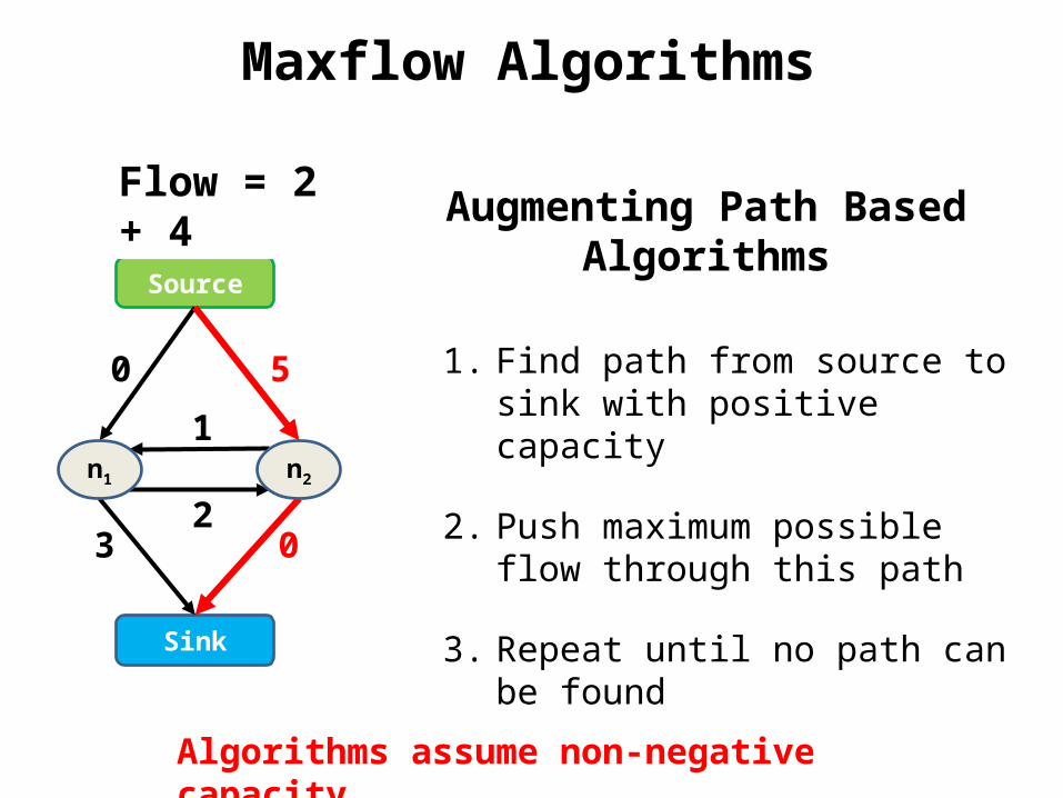
Maxflow Algorithms
Source
Sink
0
3
5
02
1
Augmenting Path Based Algorithms
1. Find path from source to sink with positive capacity
2. Push maximum possible flow through this path
3. Repeat until no path can be found
Algorithms assume non-negative capacity
Flow = 2 + 4
n1 n2
Maxflow Algorithms
Source
Sink
0
3
5
02
1
Augmenting Path Based Algorithms
1. Find path from source to sink with positive capacity
2. Push maximum possible flow through this path
3. Repeat until no path can be found
Algorithms assume non-negative capacity
Flow = 6
n1 n2

Maxflow Algorithms
Source
Sink
0
3
5
02
1
Augmenting Path Based Algorithms
1. Find path from source to sink with positive capacity
2. Push maximum possible flow through this path
3. Repeat until no path can be found
Algorithms assume non-negative capacity
Flow = 6
n1 n2
Maxflow Algorithms
Source
Sink
0
2
4
02+1
1-1
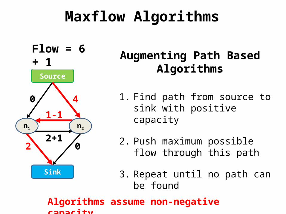
Augmenting Path Based Algorithms
1. Find path from source to sink with positive capacity
2. Push maximum possible flow through this path
3. Repeat until no path can be found
Algorithms assume non-negative capacity
Flow = 6 + 1
n1 n2

Maxflow Algorithms
Source
Sink
0
2
4
03
0
Augmenting Path Based Algorithms
1. Find path from source to sink with positive capacity
2. Push maximum possible flow through this path
3. Repeat until no path can be found
Algorithms assume non-negative capacity
Flow = 7
n1 n2
Maxflow Algorithms
Source
Sink
0
2
4
03
0
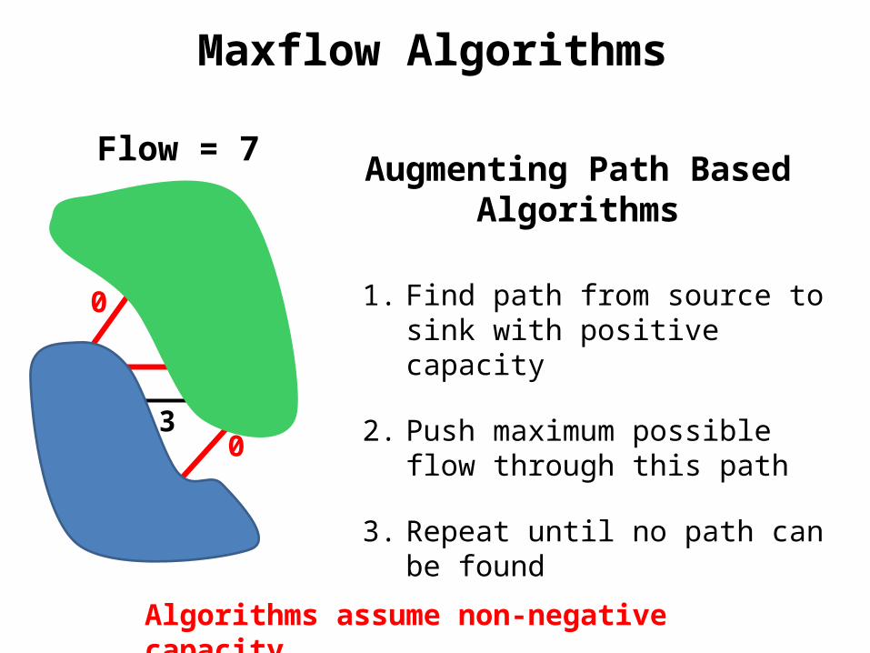
Augmenting Path Based Algorithms
1. Find path from source to sink with positive capacity
2. Push maximum possible flow through this path
3. Repeat until no path can be found
Algorithms assume non-negative capacity
Flow = 7
n1 n2
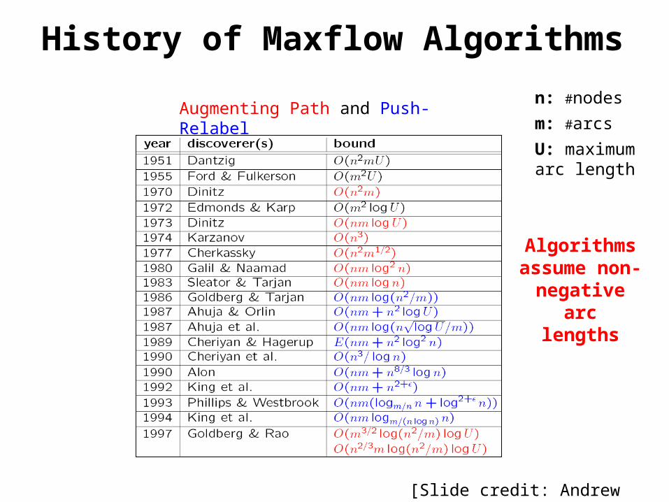
History of Maxflow Algorithms
[Slide credit: Andrew Goldberg]
Augmenting Path and Push-Relabel
n: #nodes
m: #arcs
U: maximumarc length
Algorithms assume non-negative arc
lengths

History of Maxflow Algorithms
[Slide credit: Andrew Goldberg]
Augmenting Path and Push-Relabel
n: #nodes
m: #arcs
U: maximum arc length
Algorithms assume non-negative arc
lengths
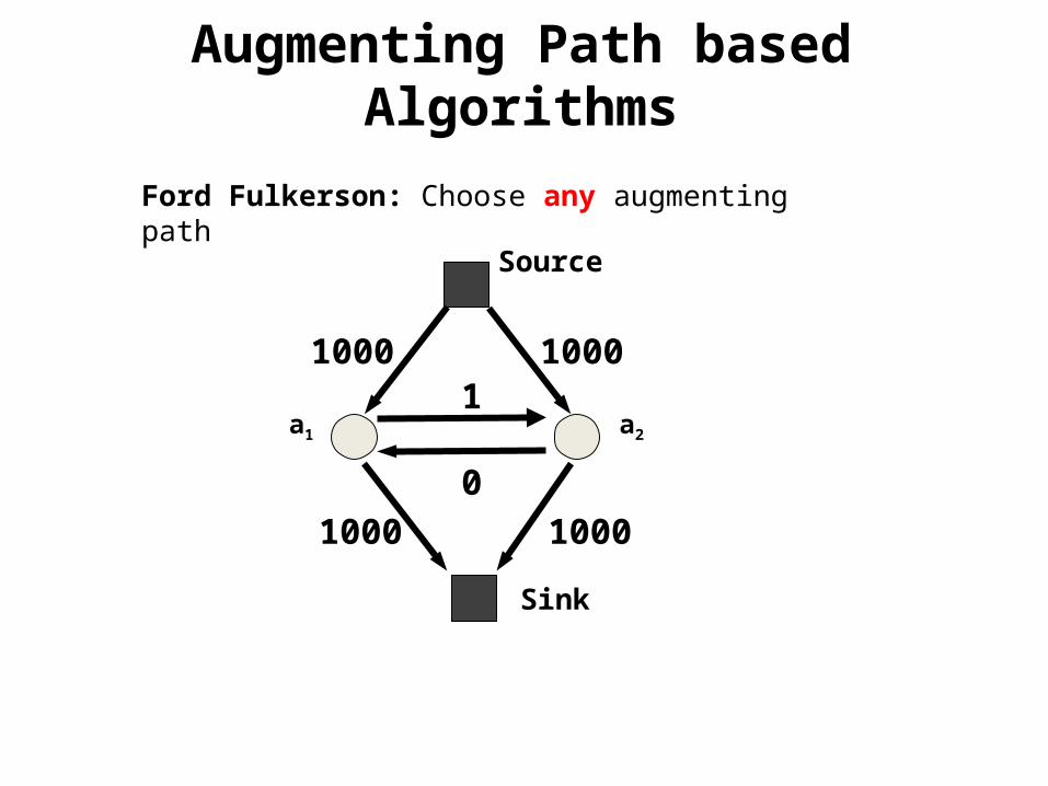
Augmenting Path based Algorithms
a1 a2
1000 1
Sink
Source
1000
1000
1000
0
Ford Fulkerson: Choose any augmenting path
a1 a2
1000 1
Sink
Source
1000
1000
1000
0
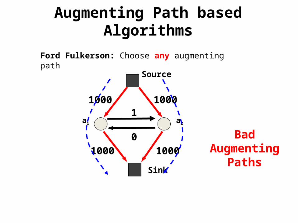
Augmenting Path based Algorithms
Bad Augmenting
Paths
Ford Fulkerson: Choose any augmenting path

a1 a2
1000 1
Sink
Source
1000
1000
1000
0
Augmenting Path based Algorithms
Bad Augmenting
Path
Ford Fulkerson: Choose any augmenting path
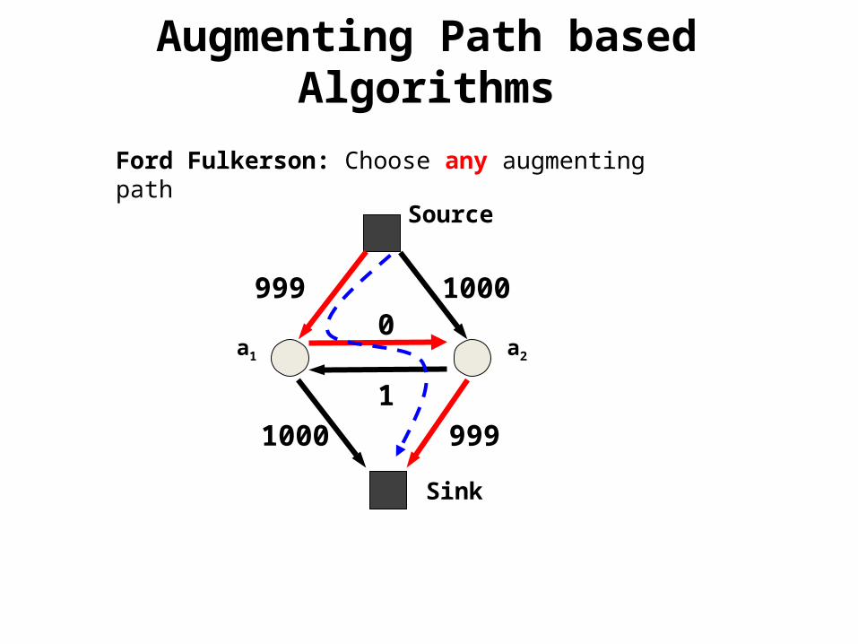
a1 a2
9990
Sink
Source
1000
1000
9991
Augmenting Path based Algorithms
Ford Fulkerson: Choose any augmenting path
a1 a2
9990
Sink
Source
1000
1000
9991
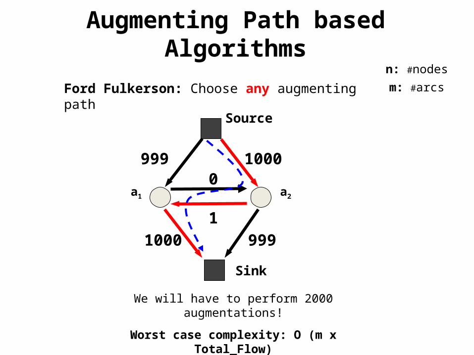
Ford Fulkerson: Choose any augmenting path
n: #nodes
m: #arcs
We will have to perform 2000 augmentations!
Worst case complexity: O (m x Total_Flow)
(Pseudo-polynomial bound: depends on flow)
Augmenting Path based Algorithms

Dinic: Choose shortest augmenting path
n: #nodes
m: #arcs
Worst case Complexity: O (m n2)
Augmenting Path based Algorithms
a1 a2
1000 1
Sink
Source
1000
1000
1000
0
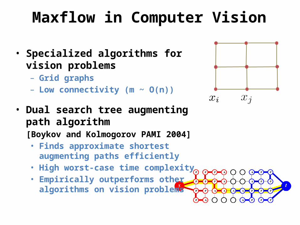
Maxflow in Computer Vision
• Specialized algorithms for vision problems– Grid graphs – Low connectivity (m ~ O(n))
• Dual search tree augmenting path algorithm[Boykov and Kolmogorov PAMI 2004]• Finds approximate shortest
augmenting paths efficiently• High worst-case time complexity• Empirically outperforms other
algorithms on vision problems
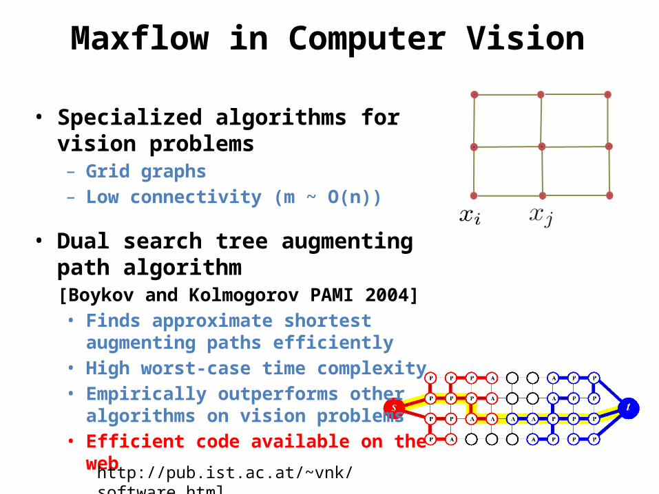
Maxflow in Computer Vision
• Specialized algorithms for vision problems– Grid graphs – Low connectivity (m ~ O(n))
• Dual search tree augmenting path algorithm[Boykov and Kolmogorov PAMI 2004]• Finds approximate shortest
augmenting paths efficiently• High worst-case time complexity• Empirically outperforms other
algorithms on vision problems• Efficient code available on the
webhttp://pub.ist.ac.at/~vnk/software.html
Outline
• Minimum Cut Problem
• Two-Label Submodular Energy Functions
• Move-Making Algorithms
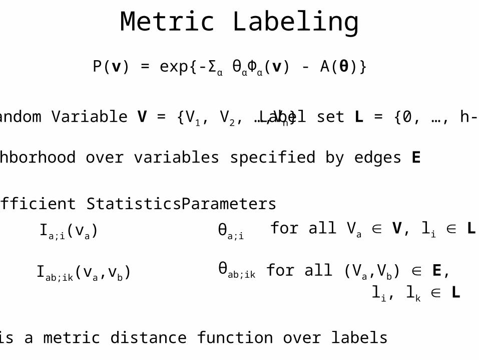
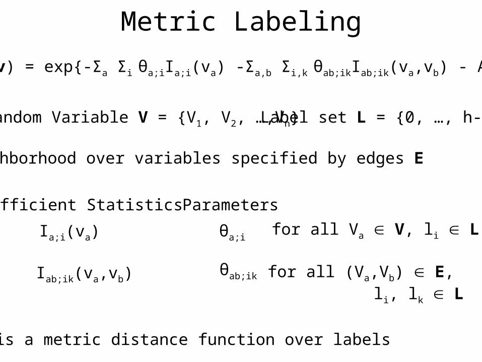
Metric Labeling
P(v) = exp{-Σα θαΦα(v) - A(θ)}
Random Variable V = {V1, V2, …,Vn}
Neighborhood over variables specified by edges E
Sufficient Statistics Parameters
Ia;i(va) θa;ifor all Va V, li L
θab;ik for all (Va,Vb) E, li, lk L
Iab;ik(va,vb)
θab;ik is a metric distance function over labels
Label set L = {0, …, h-1}
Metric Labeling
P(v) = exp{-Σa Σi θa;iIa;i(va) -Σa,b Σi,k θab;ikIab;ik(va,vb) - A(θ)}
Random Variable V = {V1, V2, …,Vn}
Neighborhood over variables specified by edges E
Sufficient Statistics Parameters
Ia;i(va) θa;ifor all Va V, li L
θab;ik for all (Va,Vb) E, li, lk L
Iab;ik(va,vb)
θab;ik is a metric distance function over labels
Label set L = {0, …, h-1}
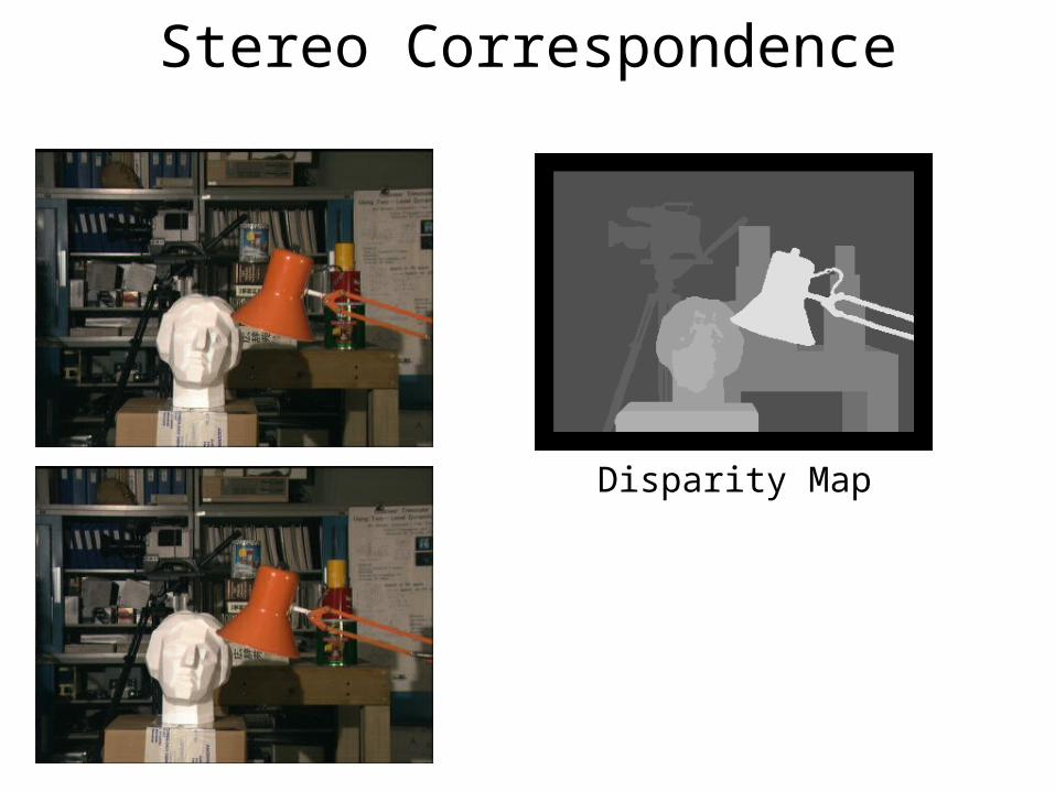
Stereo Correspondence
Disparity Map
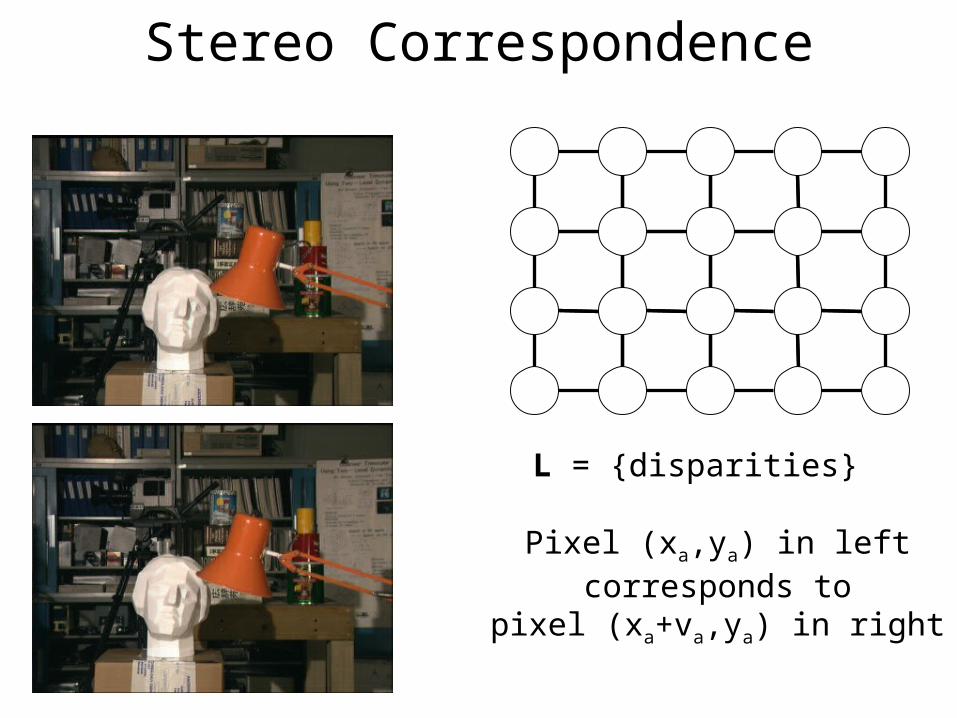
Stereo Correspondence
L = {disparities}
Pixel (xa,ya) in leftcorresponds to
pixel (xa+va,ya) in right

Stereo Correspondence
L = {disparities}
θa;i is proportional tothe difference in RGB values
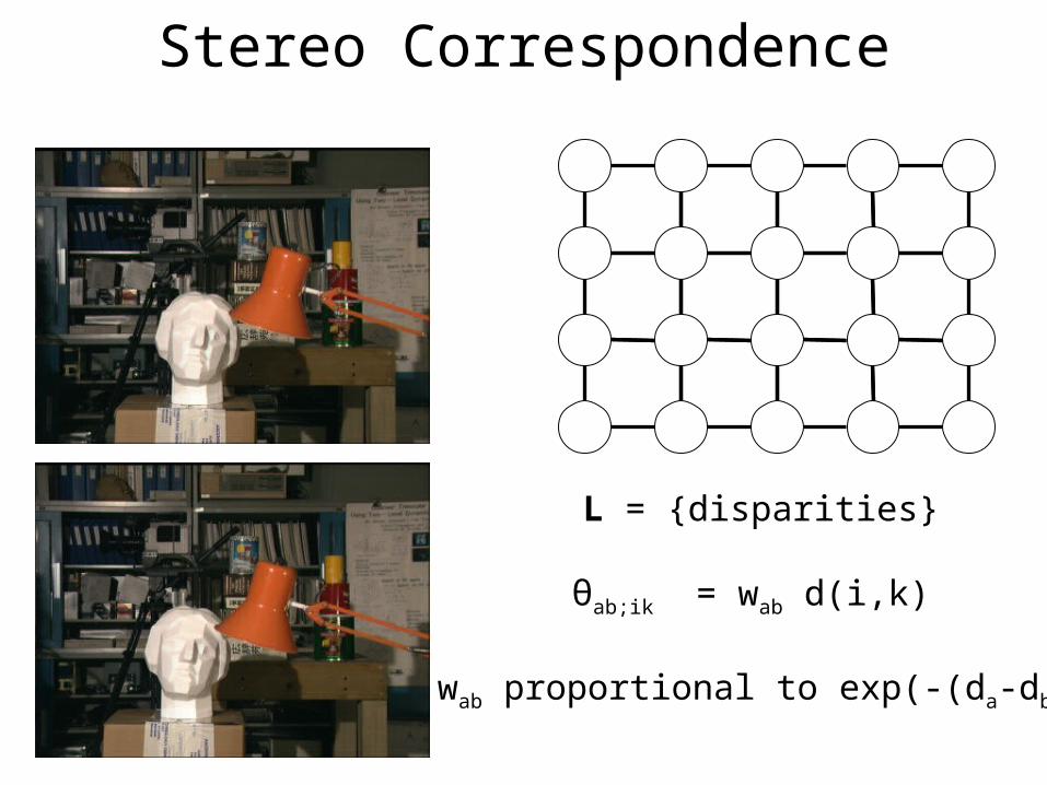
Stereo Correspondence
L = {disparities}
θab;ik = wab d(i,k)
wab proportional to exp(-(da-db)2)
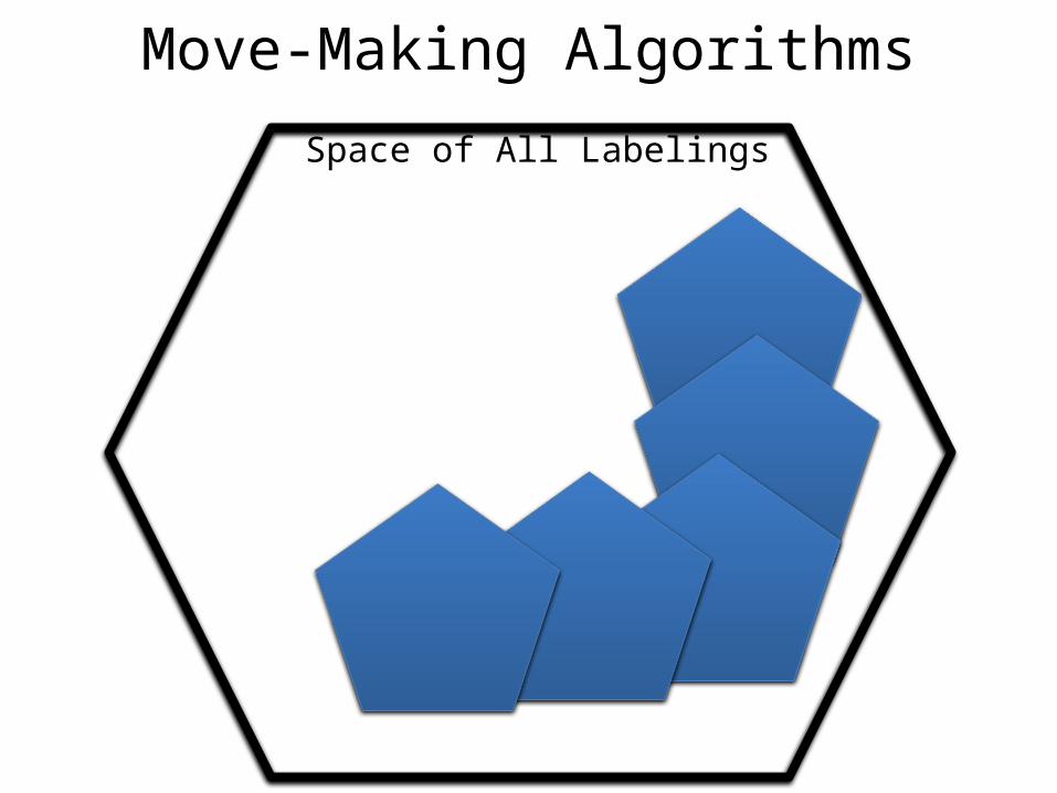
Move-Making Algorithms
Space of All Labelings
f
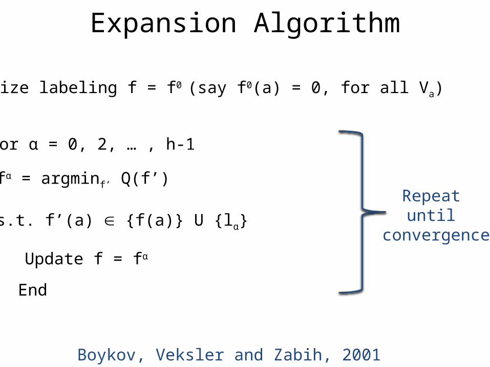
Expansion Algorithm
Initialize labeling f = f0 (say f0(a) = 0, for all Va)
For α = 0, 2, … , h-1
End
fα = argminf’ Q(f’)
s.t. f’(a) {f(a)} U {lα}
Update f = fα
Boykov, Veksler and Zabih, 2001
Repeat until
convergence
Expansion Algorithm
Variables take label lα or retain current label
Slide courtesy Pushmeet Kohli
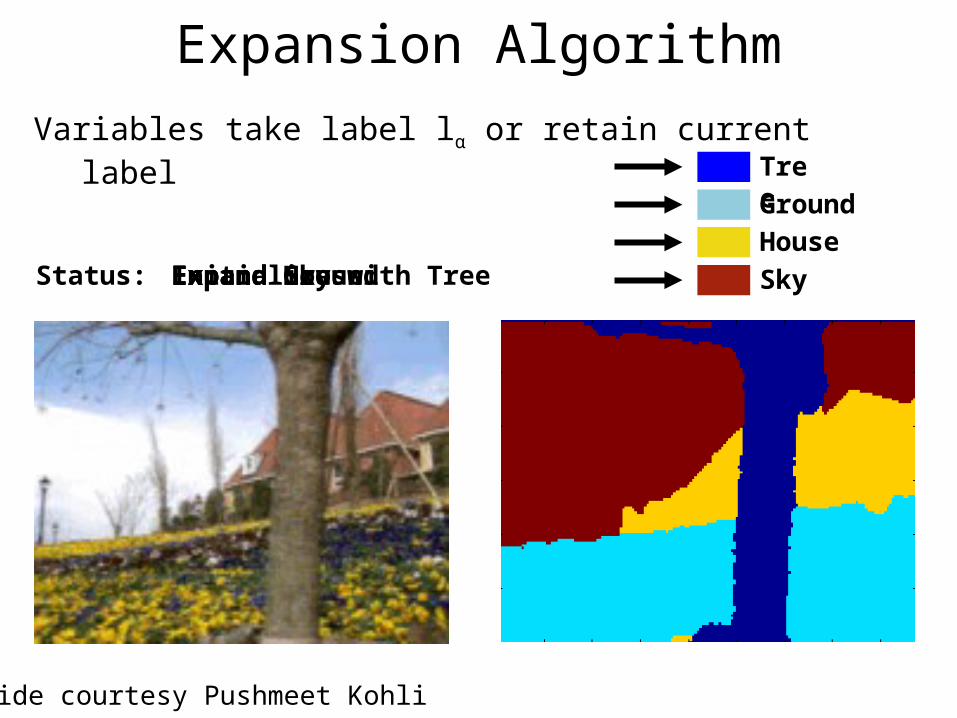
Expansion Algorithm
Sky
House
Tree
Ground
Initialize with TreeStatus: Expand GroundExpand HouseExpand Sky
Slide courtesy Pushmeet Kohli
Variables take label lα or retain current label
Expansion Algorithm
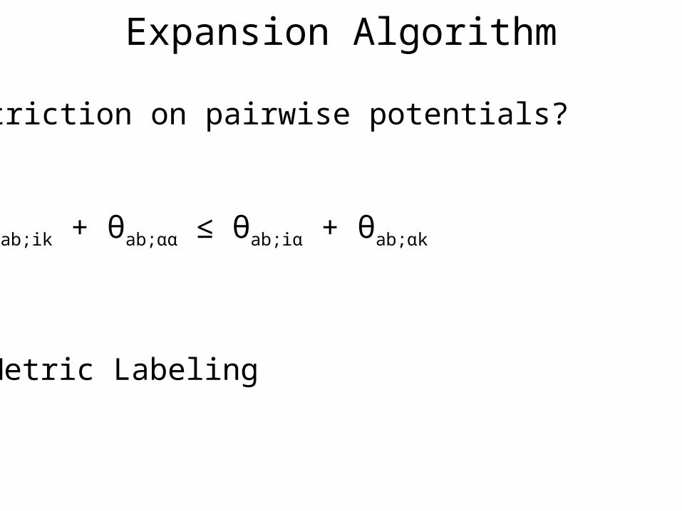
Restriction on pairwise potentials?
θab;ik + θab;αα ≤ θab;iα + θab;αk
Metric Labeling