Dr. Anjaneyulu M.V.L.R.

Professor, CED

National Institute of

Technology

Calicut, Kerala, India

Presented by

Sreelekha.M.G.

Research Scholar

Dr.K.Krishnamurthy

Assitant Professor, CED

National Institute of

Technology

Calicut, Kerala, India

1. Introduction

2. Objectives

3. Measures for evaluating transport network

4. Road network patterns and properties

5. Characterisation of transport system patterns

6. Conclusions

7. References

3

Transport system provides accessibilty

Important element in urban development

Transport system-particularly road network

Key role in the overall development of a city

Huge developmental cost

Effective utilisation is essential

Depends on connectivity and orientation

Layout and pattern of the transport system

Spatial metrics-useful quantitative information

Urban transport network efficiency analysis

Measures-help to interpret a network structure

INTRODUCTION

4

To provide a detailed review on various

indicators that can be used for road

network characterisation

To see how the indices vary among the

various patterns of road networks

OBJECTIVES

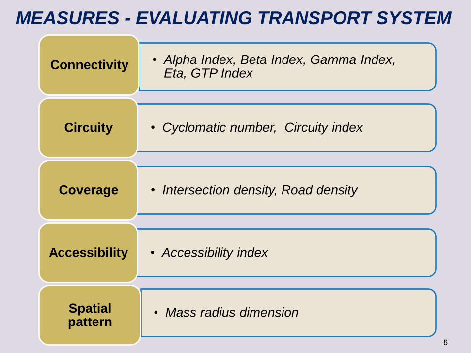
• Alpha Index, Beta Index, Gamma Index, Eta, GTP Index

Connectivity

• Cyclomatic number, Circuity index Circuity

• Intersection density, Road density Coverage

• Accessibility index Accessibility

• Mass radius dimension Spatial pattern

5

MEASURES - EVALUATING TRANSPORT SYSTEM

6

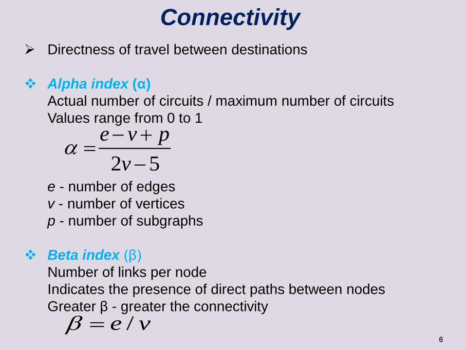
Connectivity

Directness of travel between destinations

Alpha index (α)

Actual number of circuits / maximum number of circuits

Values range from 0 to 1

e - number of edges

v - number of vertices

p - number of subgraphs

Beta index (β)

Number of links per node

Indicates the presence of direct paths between nodes

Greater β - greater the connectivity

/e v

 2 5

e v p

v

7

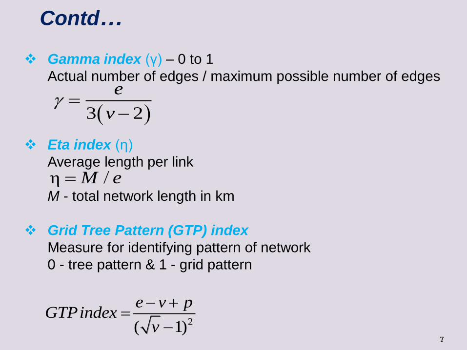
Gamma index (γ) – 0 to 1

Actual number of edges / maximum possible number of edges

Eta index (η)

Average length per link

M - total network length in km

Grid Tree Pattern (GTP) index

Measure for identifying pattern of network

0 - tree pattern & 1 - grid pattern

Contd…

   

3 2

e

v

η  /M e

2   

( 1)

e v pGTPindex

v

8

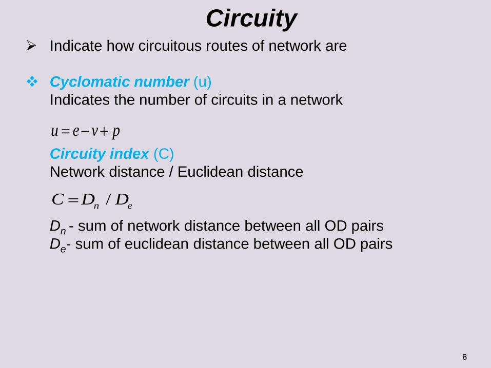
Indicate how circuitous routes of network are

Cyclomatic number (u)

Indicates the number of circuits in a network

Circuity index (C)

Network distance / Euclidean distance

Dn - sum of network distance between all OD pairs

De- sum of euclidean distance between all OD pairs

Circuity

u e v p

   /n eC D D

9

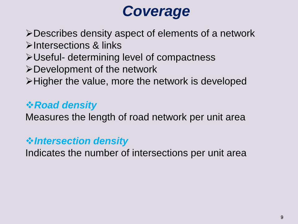
Describes density aspect of elements of a network

Intersections & links

Useful- determining level of compactness

Development of the network

Higher the value, more the network is developed

Road density

Measures the length of road network per unit area

Intersection density

Indicates the number of intersections per unit area

Coverage

10

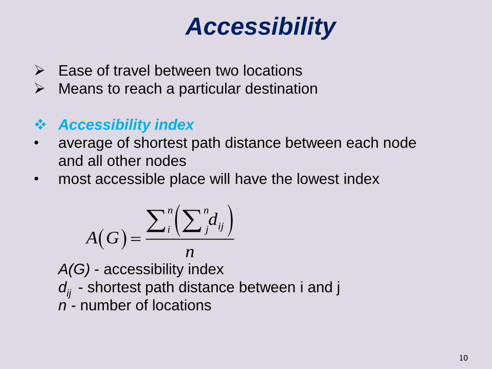
Accessibility

Ease of travel between two locations

Means to reach a particular destination

Accessibility index

• average of shortest path distance between each node

and all other nodes

• most accessible place will have the lowest index

A(G) - accessibility index

dij - shortest path distance between i and j

n - number of locations

n n

iji jd

A Gn

11

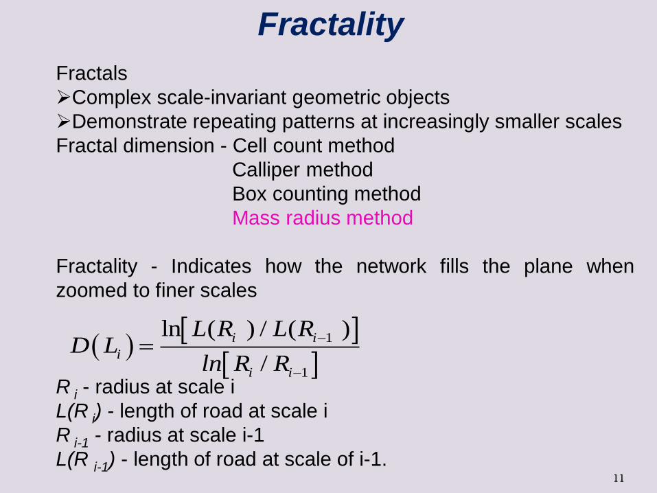
Fractality

Fractals

Complex scale-invariant geometric objects

Demonstrate repeating patterns at increasingly smaller scales

Fractal dimension - Cell count method

Calliper method

Box counting method

Mass radius method

Fractality - Indicates how the network fills the plane when

zoomed to finer scales

R i - radius at scale i

L(R i) - length of road at scale i

R i-1 - radius at scale i-1

L(R i-1) - length of road at scale of i-1.

1

1

ln  (  ) / (  )

  /

i i

i

i i

L R L RD L

ln R R

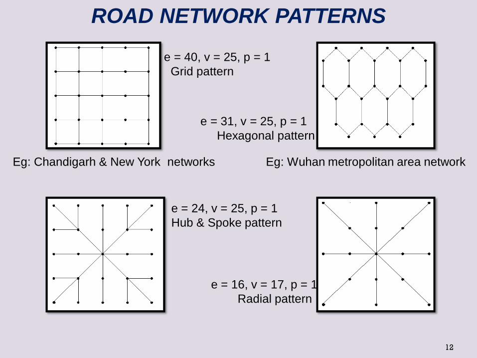
ROAD NETWORK PATTERNS

e = 40, v = 25, p = 1

Grid pattern

e = 31, v = 25, p = 1

Hexagonal pattern

e = 24, v = 25, p = 1

Hub & Spoke pattern

e = 16, v = 17, p = 1

Radial pattern

Eg: Chandigarh & New York networks Eg: Wuhan metropolitan area network

12

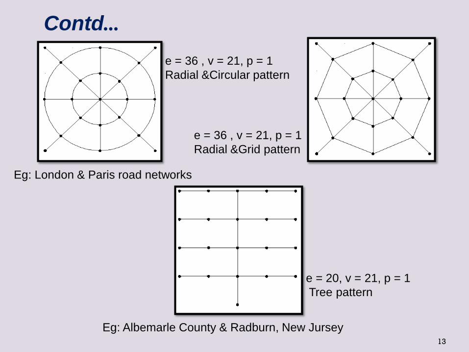
e = 36 , v = 21, p = 1

Radial &Circular pattern

e = 36 , v = 21, p = 1

Radial &Grid pattern

e = 20, v = 21, p = 1

Tree pattern

Contd...

Eg: London & Paris road networks

Eg: Albemarle County & Radburn, New Jursey 13

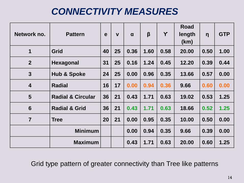
CONNECTIVITY MEASURES

Network no. Pattern e v α β ϒ

Road

length

(km)

η GTP

1 Grid 40 25 0.36 1.60 0.58 20.00 0.50 1.00

2 Hexagonal 31 25 0.16 1.24 0.45 12.20 0.39 0.44

3 Hub & Spoke 24 25 0.00 0.96 0.35 13.66 0.57 0.00

4 Radial 16 17 0.00 0.94 0.36 9.66 0.60 0.00

5 Radial & Circular 36 21 0.43 1.71 0.63 19.02 0.53 1.25

6 Radial & Grid 36 21 0.43 1.71 0.63 18.66 0.52 1.25

7 Tree 20 21 0.00 0.95 0.35 10.00 0.50 0.00

Minimum 0.00 0.94 0.35 9.66 0.39 0.00

Maximum 0.43 1.71 0.63 20.00 0.60 1.25

Grid type pattern of greater connectivity than Tree like patterns

14

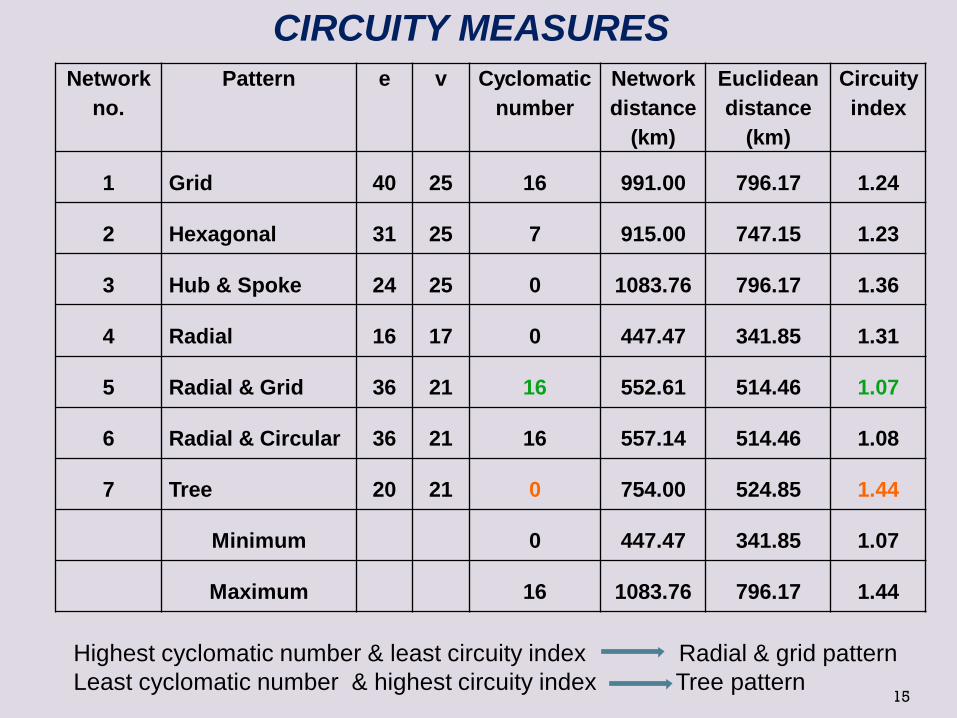
CIRCUITY MEASURES

Network

no.

Pattern e v Cyclomatic

number

Network

distance

(km)

Euclidean

distance

(km)

Circuity

index

1 Grid 40 25 16 991.00 796.17 1.24

2 Hexagonal 31 25 7 915.00 747.15 1.23

3 Hub & Spoke 24 25 0 1083.76 796.17 1.36

4 Radial 16 17 0 447.47 341.85 1.31

5 Radial & Grid 36 21 16 552.61 514.46 1.07

6 Radial & Circular 36 21 16 557.14 514.46 1.08

7 Tree 20 21 0 754.00 524.85 1.44

Minimum 0 447.47 341.85 1.07

Maximum 16 1083.76 796.17 1.44

Highest cyclomatic number & least circuity index Radial & grid pattern

Least cyclomatic number & highest circuity index Tree pattern

15

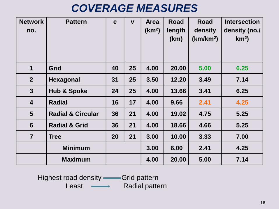
COVERAGE MEASURES Network

no.

Pattern e v Area

(km2)

Road

length

(km)

Road

density

(km/km2)

Intersection

density (no./

km2)

1 Grid 40 25 4.00 20.00 5.00 6.25

2 Hexagonal 31 25 3.50 12.20 3.49 7.14

3 Hub & Spoke 24 25 4.00 13.66 3.41 6.25

4 Radial 16 17 4.00 9.66 2.41 4.25

5 Radial & Circular 36 21 4.00 19.02 4.75 5.25

6 Radial & Grid 36 21 4.00 18.66 4.66 5.25

7 Tree 20 21 3.00 10.00 3.33 7.00

Minimum 3.00 6.00 2.41 4.25

Maximum 4.00 20.00 5.00 7.14

Highest road density Grid pattern

Least Radial pattern

16

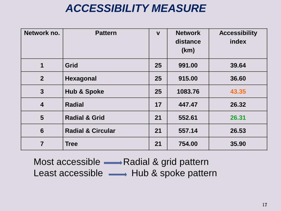
ACCESSIBILITY MEASURE

Most accessible Radial & grid pattern

Least accessible Hub & spoke pattern

Network no. Pattern v Network

distance

(km)

Accessibility

index

1 Grid 25 991.00 39.64

2 Hexagonal 25 915.00 36.60

3 Hub & Spoke 25 1083.76 43.35

4 Radial 17 447.47 26.32

5 Radial & Grid 21 552.61 26.31

6 Radial & Circular 21 557.14 26.53

7 Tree 21 754.00 35.90

17

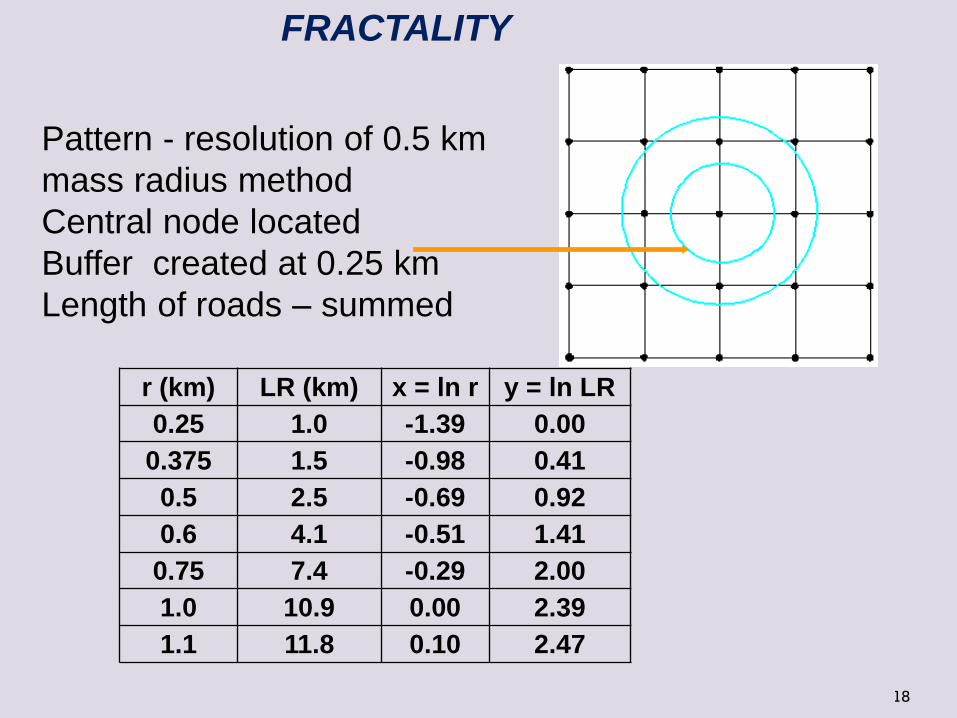
r (km) LR (km) x = ln r y = ln LR

0.25 1.0 -1.39 0.00

0.375 1.5 -0.98 0.41

0.5 2.5 -0.69 0.92

0.6 4.1 -0.51 1.41

0.75 7.4 -0.29 2.00

1.0 10.9 0.00 2.39

1.1 11.8 0.10 2.47

18

FRACTALITY

Pattern - resolution of 0.5 km

mass radius method

Central node located

Buffer created at 0.25 km

Length of roads – summed

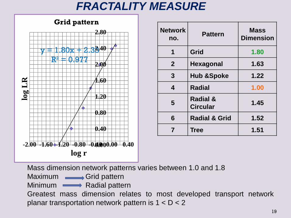
FRACTALITY MEASURE

Network

no. Pattern

Mass

Dimension

1 Grid 1.80

2 Hexagonal 1.63

3 Hub &Spoke 1.22

4 Radial 1.00

5 Radial &

Circular 1.45

6 Radial & Grid 1.52

7 Tree 1.51

Mass dimension network patterns varies between 1.0 and 1.8

Maximum Grid pattern

Minimum Radial pattern

Greatest mass dimension relates to most developed transport network

planar transportation network pattern is 1 < D < 2 19

y = 1.80x + 2.33

R² = 0.977

0.00

0.40

0.80

1.20

1.60

2.00

2.40

2.80

-2.00 -1.60 -1.20 -0.80 -0.40 0.00 0.40

log

LR

log r

Grid pattern

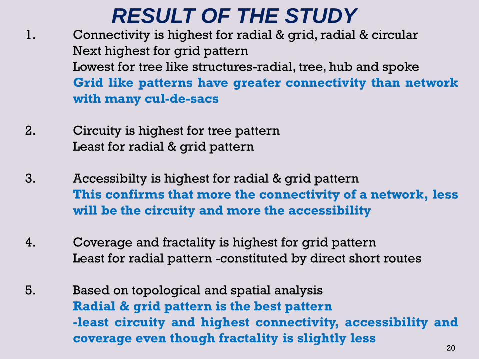
RESULT OF THE STUDY

1. Connectivity is highest for radial & grid, radial & circular

Next highest for grid pattern

Lowest for tree like structures-radial, tree, hub and spoke

Grid like patterns have greater connectivity than network

with many cul-de-sacs

2. Circuity is highest for tree pattern

Least for radial & grid pattern

3. Accessibilty is highest for radial & grid pattern

This confirms that more the connectivity of a network, less

will be the circuity and more the accessibility

4. Coverage and fractality is highest for grid pattern

Least for radial pattern -constituted by direct short routes

5. Based on topological and spatial analysis

Radial & grid pattern is the best pattern

-least circuity and highest connectivity, accessibility and

coverage even though fractality is slightly less 20

21

•Batty, M. & Longley, P. (1994). Fractal Cities, Academic Press, San

Diego, CA.

•Bento, A.M., Cropper, M.L., Mobarak, A.M., and Vinha, K. (2003). The

impact of urban spatial structure on travel demand in the United States,

World Bank policy research working paper, 3007.

•Cervero, R. & Kockelman, K. (1997). Travel demand and the 3Ds:

Density, Diversity and Design, Transportation Research D, 2(3), 199–

219.

•El-Geneidy, A. & Levinson, D. (2007). Network Circuity and Journey to

Work, Presented at the University Transport Study Group Conference at

Harrowgate, England, January 3-5.

•Kansky, K. (1963). Structure of Transportation Networks: Relationships

between Network Geometry and Regional Characteristics, Ph. D. thesis,

University of Chicago, Research Paper No. 84.

•Noda, H. (1996). A Quantitative Analysis on the Patterns of Street

Networks using Mesh Data System, City Planning Review, 202, 64-72 (in

Japanese).

•Rodrigue, J. P., Comtois, C., and Slack, B. (2006). The Geography of

Transport System, London; New York, Routledge.

NIT, Calicut 22

23