Prepared for submission to JHEP TTP13-005, SFB/CPP-13-07

O(α2s) corrections to fully-differential top quark decays

Mathias Brucherseifer,1 Fabrizio Caola2 and Kirill Melnikov2

1Institut fur Theoretische Teilchenphysik, Karlsruhe Institute of Technology (KIT), Germany2Department of Physics and Astronomy, Johns Hopkins University, Baltimore, USA

E-mail: mathias.brucherseifer@kit.edu, caola@pha.jhu.edu, melnikov@pha.jhu.edu

Abstract: We describe a calculation of the fully-differential decay rate of a top quark to a massless

b-quark and a lepton pair at next-to-next-to-leading order in perturbative QCD. Technical details of

the calculation are discussed and selected results for kinematic distributions are shown.

Contents

1 Introduction 1

2 The set up 2

3 Phase-spaces for various sub-processes in top decays 6

4 Singular limits 12

5 How to treat spin-correlations consistently in the NNLO computation 15

6 Results 17

7 Conclusions 19

A Tree-level amplitudes 20

B Calculation of one-loop integrals for the soft limit 22

1 Introduction

Top quark physics at the LHC is benefiting from huge samples of events that can be used to systemati-

cally explore many interesting properties of the top quark such as its mass, its production cross-section

and the structure of its couplings to other Standard Model particles, including the Higgs boson. Many

of such studies require a good understanding of the kinematics of top quark decay products that are

affected by QCD radiative corrections.

The next-to-leading (NLO) QCD corrections to the top quark total decay width and many kine-

matic distributions are known since long ago [1–3]. The electroweak corrections have been computed

in Refs. [4]. The fully differential computation of corrections to the top quark width at next-to-leading

order was reported in recent years in Refs. [5–7]; it was performed in the context of NLO QCD calcu-

lations for a number of processes in top quark physics where radiative corrections to the production

and decay stages are incorporated consistently [5–11].

While the NLO QCD description of many hadron collider processes provides quite a reasonable

approximation, for some processes it may be useful to improve on that and compute the next-to-

next-to-leading order (NNLO) QCD corrections. Top quark pair production in hadron collisions is

one of such processes and computations of NNLO QCD corrections to pp → tt are well underway

[12–14]. So far these calculations are performed for stable top quarks and address the total cross-

section but, eventually, they will mature enough to include also top quark decays in the narrow

width approximation. This approximation, when done consistently, includes radiative corrections to

production and decay stages and gives an excellent description of the process pp → W+W−bb at

NLO QCD [15, 16], as was shown explicitly in Ref. [17]. There is no doubt that the narrow width

approximation will work very well also at next-to-next-to-leading order, once all relevant corrections

– 1 –

to the production and decay stages are accounted for at a fully-differential level. The goal of this

paper is to provide a fully-differential NNLO QCD calculation for the top quark width.

The NNLO QCD radiative corrections to the total width of the top quark were computed in a

number of papers [18–21] and, more recently, NNLO QCD corrections to W -helicity fractions were

reported in Ref. [22]. However, NNLO QCD corrections to other kinematic distributions in top decays

were unknown. We note that very recently NNLO QCD radiative corrections to top quark decay at a

fully differential level were computed in Ref. [23], using a slicing method inspired by soft-collinear effec-

tive theory [24]. Our computation employs a totally different method and, as such, is complementary

to Ref. [23].

A different phenomenological motivation for this computation comes from a similarity between

two processes, t→ b+e+ +ν and b→ u+e−+ ν. This similarity implies that if NNLO QCD radiative

corrections are known for an arbitrary invariant mass of the lepton pair, i.e. beyond the narrow W -

width approximation, they can be immediately applied to the calculation of NNLO QCD corrections to

moments of kinematic distributions in the b→ u semileptonic transition. Since the b→ u decay suffers

from significant background from b → c transition, the inclusive rate for b → u is of little help for

improving the precision with which the CKM matrix element |Vub| can be extracted from experimental

measurements. On the other hand, the knowledge of radiative corrections to moments of kinematic

distributions with cuts on the electron energy and hadronic invariant mass is useful for constructing a

theoretical framework to extract |Vub|, see e.g. Refs. [25–28]. The computational framework that we

develop in the current paper is immediately applicable to the calculation of these moments.

The other goal of this paper is to contribute to the development of a robust computational scheme

that will be applicable to any collider process at NNLO QCD. A promising way towards such a general

scheme was described by Czakon [29, 30] who suggested to combine ideas of sector decomposition [31–

33] and the Frixione-Kunszt-Signer (FKS) phase-space partitioning [34]. This computational scheme

was further discussed in Ref. [35] where it was applied to the calculation of NNLO QED corrections

to Z → e+e−. In this paper, we employ these methods to compute NNLO QCD radiative corrections

to top quark decay. From the methodological point of view, top quark decay t→ b+ e+ + ν provides

an interesting case where the structure of soft and collinear singularities is relatively simple, yet a

massive colored particle in the initial state leads to a computational complexity.

The paper is organized as follows. In the next Section, we discuss the general set up of the

computation. In Section 3 we explain how the phase-space for various subprocesses related to top

quark decays can be parametrized to enable the extraction of infra-red and collinear singularities. In

Section 4 we discuss the singular limits of various amplitudes required for our computation. In Section 5

we explain some peculiarities that arise when we try to keep all momenta of external particles in four

dimensions, yet use dimensional regularization consistently. In Section 6 we describe the results of

the calculation and show some kinematic distributions. In Section 7 we present our conclusions.

Finally, we give explicit expressions for tree amplitudes employed in our calculation in Appendix A

and show how to compute one-loop master integrals needed in the constructions of one-loop soft limits

in Appendix B.

2 The set up

As we already mentioned in the Introduction, our goal in this paper is to compute NNLO QCD

corrections to the fully differential decay rate of the top quark t(pt) −→ b(pb) + νe(p5) + e+(p6).

Throughout the paper, we work in the top quark rest frame. The decay to e+ν is facilitated by an

emission of a W -boson, which can be either on or off the mass-shell. The interaction of the virtual W

– 2 –

boson with the neutrino-positron pair W → ν(p5) + e+(p6) is described by the vertex

igW√2〈5|γµ|6], (2.1)

where we use the bra and ket notation for massless spinors with definite helicities. We employ the

standard notation u+(pi) = |pi,+〉 = |i〉, u−(pi) = |pi,−〉 = |i] and note that further discussion of

spinor-helicity methods can be found in the review Ref. [36].

We are interested in the NNLO QCD corrections to semileptonic top quark decay. To compute

these radiative corrections, we require the following ingredients

• two-loop virtual corrections to t→ b+ ν + e+;

• one-loop virtual corrections to t→ b+ g + ν + e+;

• tree-level double-real emission contributions to the decay rate, t → b + g + g + ν + e+ and

t→ b+ qq + ν + e+.

We note that most of the required contributions are available in the literature. Indeed, two-

loop QCD virtual corrections to t → Wb can be obtained from an analytic computation of similar

corrections to b → W ∗u, reported recently by a number of authors [37–41]. One-loop amplitudes for

the t → b + g + ν + e+ process can be extracted from Ref. [6]. Double-real emission amplitudes for

gluons and quarks are not known in a compact analytic form but can be easily calculated using the

spinor-helicity formalism.

However, similar to other NNLO computations, the availability of required amplitudes does not

make it obvious how to arrive at a physical answer. This happens because of infra-red and collinear

singularities that need to be extracted from individual contributions before integrating over phase-

spaces of final-state particles. Until recently, the two methods1 that were used to extract singularities

in practical NNLO computations were sector decomposition [31–33] and antenna subtraction [46, 47].

Both of these methods were developed further in recent years [48, 49] with the goal to make them

applicable to more complex processes than previously considered.

The method that we use in this paper was suggested by Czakon [29, 30] (see also [35]), who

pointed out that a combination of sector decomposition [31–33] and the FKS phase-space partitioning

[34] allows to resolve overlapping soft and collinear singularities in a universal way. We note that from

the technical point of view, the case of top quark decay is particularly simple since no complicated

phase-space partitioning is, in fact, required. Indeed, singularities in matrix elements occur when

emitted gluons are either soft or collinear to other massless partons. Since there are only three strongly

interacting massless particles in double-real emission amplitudes for top decays, there is just one triple-

collinear limit and no need for angular partitioning arises. The soft singularities are disentangled by

ordering gluons with respect to their energies and by removing the corresponding 1/2! factor from the

phase-space. Note that this argument needs to be modified for sub-processes with two quarks in the

final state and we explain how to do it in what follows.

We now remind the reader about the general approach to fully differential NNLO QCD compu-

tations based on sector decomposition and phase-space partitioning [29, 30] (see also [35]). The main

idea is to express the phase-space for the final state particles through suitable unit-hypercube variables

that make the singular behavior of scattering amplitudes manifest. Once this is accomplished, it is easy

1Other approaches to NNLO calculations are discussed in [42–44]. Some phenomenological applications can be found

in [45].

– 3 –

to construct subtraction terms for real emission processes by using expansion in plus-distributions. To

be specific, we consider a double-real emission contribution to the differential decay rate of the top

quark

Γ(RR)t =

∫dLips |M(p)|2J(p), (2.2)

where dLips is a phase-space for t→ b+ g+ g+ e+ + ν,M(p) is the decay amplitude and J(p) is

a measurement function that depends on momenta of final state particles p. We assume that a map

of the phase-space onto a unit hypercube is found; variables that parametrize the map are denoted as

x. As we will show below, it is possible to re-write Eq.(2.2) as

Γ(RR)t =

NS∑i=1

Γ(RR,i)t , Γ

(RR,i)t =

Nps∏j=1

1∫0

dxj

x1+a

(i)j ε

j

Fi(ε, x) (2.3)

where NS is the number of sectors, ε = (4− d)/2 is the parameter of dimensional regularization, Nps

is the number of independent variables required to parametrize the phase-space, and the function F

is the product of the scattering amplitude squared, sector-dependent powers of singular variables and

the phase-space weight Psw(x) that may include the measurement function

Fi(x) = xb11 xb22 ..x

bNpsNps|M(p)|2 Psw(x). (2.4)

The important property of these functions Fi is that limits exist at each potentially singular point

xj = 0,

limxj=0

Fi(.., xj , ..) = Fi(.., 0, ..) 6=∞. (2.5)

The existence of limits Eq.(2.5) allows us to re-write Eq.(2.3) in an explicitly integrable form by

employing the decomposition in plus-distributions

1

x1+aε= − 1

aεδ(x) +

∞∑n=0

(−εa)n

n!

[lnn(x)

x

]+

. (2.6)

Substituting this expansion into Eq.(2.3) and collecting terms of the same order in ε, we obtain

explicitly integrable terms that can be divided into two broad categories,

1∫0

dxilnn(xi) (F (.., xi, ..)− F (.., 0, ..))

xiand

1∫0

dxiδ(xi)F (.., 0, ..). (2.7)

It is easy to recognize that the first integral in the above equation contains a “subtraction term”

and the second integral defines an “integrated subtraction term”, if the language familiar from NLO

QCD computations is borrowed. It is remarkable that, in the described framework, the subtraction

terms are obtained automatically, once a proper parametrization of the phase-space is found and the

expansion in plus-distributions is performed. We also note that any subtraction term depends on the

function F (x1, .., xNps) at such values of xi for which at least one of the singular variables vanishes.

These kinematic points correspond to universal soft and collinear limits of scattering amplitudes so

that F (.., xi = 0, ..) can be calculated in a process-independent way. In what follows, we discuss

essential elements of this construction such as the phase-space parametrization and singular limits of

amplitudes.

– 4 –

Before proceeding to that discussion, we explain some subtleties that arise when one-loop correc-

tions to the process t→ b+ g + e+ + ν are analyzed within this framework. In this case, the singular

part of the phase-space is parametrized in terms of two variables, x1 and x2, that describe the energy

of the gluon g and the relative angle between the gluon and the b-quark, respectively. The contribution

to the top quark decay rate is given by the integral

1∫0

dx1

x1+2ε1

dx2

x1+ε2

[x21x2]2Re

[M1−loop

t→bge+νM(0),∗t→bge+ν

]..., (2.8)

where ellipses stand for other non-singular phase-space factors. While the integrand in Eq.(2.8) sug-

gests that singularities can be isolated by constructing an expansion in plus-distributions, it is in fact

not possible to do that right away. The reason is that the one-loop amplitude M1−loopt→bge+ν has branch

cuts in the limits x1 → 0 and x2 → 0 and we must account for them when constructing the expansion

of the integrand in plus-distributions. To accomplish that, we write

[x21x2]

[M1−loop

t→bge+νM(0),∗t→bge+ν

]∼ F1(x1, x2, ..) + (x2

1x2)−εF2(x1, x2, ..), (2.9)

where the two functions F1,2 are free from branch cuts in x1,2 → 0 limits.

The calculation of real-virtual corrections now proceeds as follows. We insert Eq.(2.9) into

Eq.(2.8), combine non-integer powers of x1,2 and expand in plus-distributions. Upon doing so, we

find a variety of terms that are similar to what we showed in Eq.(2.7). However, in this case the

integrand is written in terms of F1(x1, x2) and F2(x1, x2) and we need a prescription that will allow

us to compute these functions from scattering amplitudes. To understand how this is done, note that

F1,2(x) may appear in the integrand with one or both of its arguments set to zero, which corresponds

to soft or collinear kinematics of the final state gluon. To compute F1,2 in those cases, we need to

investigate[M1−loop

t→bge+νM(0),∗t→bge+ν

]in soft and collinear limits. Consider first the soft limit, x1 → 0.

In this case, the interference of the one-loop and tree matrix elements reads

limx1→0

2Re[M1−loop

t→bge+νM(0),∗t→bge+ν

]= g2

sCFStb

(2Re

[M1−loop

t→be+νM(0),∗t→be+ν

])+ g2

sCAS(1)tb

[M(0)

t→be+νM(0),∗t→be+ν

],

(2.10)

where Stb and S(1)tb are tree and one-loop eikonal factors, respectively. We note that in the right hand

side of Eq.(2.10), the dependence of the one-loop amplitude on the momentum of the soft gluon is

entirely contained in the eikonal factors. To identify F1,2 at vanishing value of x1, it is important to

realize that the leading-order eikonal factor Stb is free from branch cuts while the one-loop eikonal factor

S(1)tb may (and in fact does) contain them. We conclude that, in the soft limit x1 → 0, the first term on

the right hand side in Eq.(2.10) matches to F1(0, x2) and the second term to F2(x1 = 0, x2)(x21x2)−ε.

A similar situation occurs in the collinear limit x2 → 0. In this case

limx2→0

[M1−loop

t→bge+νM(0),∗t→bge+ν

]=

g2s

pb · pg

(P

(0)b→bg

[M1−loop

t→be+νM(0),∗t→be+ν

]+ P

(1)b→bg

[M(0)

t→be+νM(0),∗t→be+ν

]),

(2.11)

where P(0,1)b→bg are the tree- and one-loop splitting functions; these functions can be derived from collinear

limits of scattering amplitudes described in Ref. [50]. Similar to the soft limit, the tree-level splitting

function P(0)b→bg does not contain any branch cut in x2 → 0 limit, while the one-loop splitting function

– 5 –

does. Hence, the first term on the right-hand side in Eq.(2.11) is identified with F1(x1, x2 = 0) and

the second one with (x21x2)−εF2(x1, x2 = 0).

If x1 and x2 are both non-vanishing, we can re-write combinations of F1(x1, x2) and F2(x1, x2) that

appear in the integrand for the rate, through the one-loop matrix element interfered with the tree-level

amplitude, using Eq.(2.9). The one-loop amplitude for the t→ b+ g+ e+ + ν that we require, can be

extracted from Ref. [6], where Wt production in bg fusion is discussed.2 For our purpose, the relevant

amplitudes need to be crossed to describe the t→ b+ g +W+ channel. Finally, the evaluation of the

one-loop amplitude for t→ b+g+e++ν process requires master integrals; they can be computed using

the program QCDLoops [52]. We found, however, that results of this program become unreliable in

extreme kinematic limits; for example when the momentum of the gluon in the final state becomes very

small Eg ∼< 10−8mt. To overcome this difficulty, we independently implemented all master integrals

relevant for the computation of the one-loop amplitude for t→ b+ g+ e+ + ν using analytic formulas

provided in Refs. [52, 53]. Our implementation allows us to employ quadruple precision and to reach

very small gluon energies Eg ∼ 10−12mt and very small opening angles between the bottom quark

and the gluon.

The importance of reaching small energies and angles follows from Eq.(2.7) which shows that

integration over hypercube variables x should, in principle, be performed on the interval xi ∈[0, 1]. This implies that full matrix elements that contribute to the function F (x) must be evaluated

at vanishingly small values of x. It is, of course, impossible to compute them at x = 0 and we

need to introduce additional regularization. Following Refs. [29, 30] we provide this regularization

by discarding such points in x-space where the product of singular variables is smaller than a

user-defined parameter δ. For example, for double-real emission corrections where four variables are

singular, we require x1x2x3x4 > δ, while for the single-emission contributions we require x1x2 > δ.

Values of δ that we use range from 10−7 to 10−12, where extremely small values are employed to test

the independence of final results on the cut-off parameter and the cancellation of infra-red divergences.

For phenomenological calculations we find that values of δ ∼ 10−7− 10−9 are small enough to provide

reasonable results for the second order corrections.

Finally, we note that Eq.(2.7) allows us to compute arbitrary kinematic distributions in a single

run of the code. We only need to determine the kinematics of the event – which is uniquely defined

for a given set of x-variables – and assign the relevant weight to a particular bin in a histogram that

we want to compute. We do this each time the function F (x) is calculated. Such implementation

is standard for how subtraction procedure is employed in parton level Monte-Carlo event generators

both at next-to-leading order (see e.g. Ref. [51] ) and beyond [54].

3 Phase-spaces for various sub-processes in top decays

In this Section, we discuss the phase-space parametrization for the various sub-processes related to top

quark decays. We start with the leading order phase-space and then proceed to phase-spaces with one

and two additional gluons in the final state. We also address the parametrization of the phase-space

for t→ b+ qq + e+ + ν since it differs from the two-gluon case in important details.

The leading order process that we deal with is t → b + W ∗(e+ + ν), where the W -boson can be

off the mass shell. While the W off-shellness is not an important effect for top quark decays, our

reasons for doing the calculation this way is explained in the Introduction. To account for the W

2 We use the Fortran77 implementation of this amplitude in the MCFM program [51]. We slightly extend it to allow

the use of quadruple precision in Fortran90.

– 6 –

off-shellness in a systematic way, it is convenient to include the Breit-Wigner propagator from the

scattering amplitude into the definition of the phase-space. We write

dΠbe+ν =dp2

W

2π

Lips(t→ bW ∗)dLips(W ∗ → νl+)

(p2W −m2

W )2 +m2WΓ2

W

, (3.1)

where Lips stands for Lorentz-invariant phase-spaces for indicated final states, p2W is the invariant

mass of the lepton pair and ΓW is the W -decay width. We remove the Breit-Wigner distribution by

changing variables

p2W = m2

W +mWΓW tan ξ, (3.2)

so that1

2π

dp2W

(p2W −m2

W )2 +m2WΓ2

W

=dξ

2πmWΓW. (3.3)

The kinematics of the process implies a restriction on the invariant mass of the lepton pair, 0 < p2W < m2

t .

To account for it, we re-map ξ onto the (0, 1) interval by defining ξ = ξmin + (ξmax − ξmin)x7. We

obtain1

2π

dp2W

(p2W −m2

W )2 +m2WΓ2

W

= NBW dx7, (3.4)

where

NBW =ξmax − ξmin

2πmWΓW, ξmin = − arctan

mW

ΓW, ξmax = arctan

[m2t −m2

W

mWΓW

]. (3.5)

After generating the invariant mass of the lepton pair using Eq.(3.4) , we obtain lepton and neutrino

momenta in the W ∗ rest frame in the standard way

pν,l =

√p2W

2(1,±~nl), (3.6)

where ~nl = (sin θ5 cosϕ5, sin θ5 sinϕ5, cos θ5). Redefining angular variables,

cos θ5 = 1− 2x8, ϕ5 = 2πx9, (3.7)

we re-write the dilepton phase-space as

dLips(W ∗ → νl+) =dx8dx9

8π. (3.8)

We note that we treat the lepton-neutrino phase-space as four-dimensional, even in higher orders

of QCD perturbation theory where infra-red and collinear divergences require analytic continuation

of the space-time dimensionality. It is intuitively clear that it should be possible to do so because

lepton momenta are infra-red safe observables. However, some subtleties arise when the computation

is organized this way. We discuss them in Section 5.

Finally, we describe the parametrization of the t→ bW ∗ phase-space. We work in the rest frame

of the decaying top quark and define the z-axis by aligning it with the momentum of the b-quark. The

momenta read

pt = mt(1, 0, 0, 0), pb = Eb(1, ~nb), ~nb = (0, 0, 1). (3.9)

The energy of the b-quark is given by

Eb =m2t − p2

W

2mt. (3.10)

– 7 –

It is easy to find the leading order phase-space for t→ bW ∗ decay. It reads

Lips(t→ bW ) =1

8π

(1− p2

W

m2t

)Υ(ε) =

Emax

4πmtΥ(ε), (3.11)

where Emax = Eb is the maximal energy of the b-quark for fixed invariant mass of the lepton pair and

Υ(ε) =Γ(1− ε)Γ(2− 2ε)

(E2

max

π

)−ε= 1 +O(ε). (3.12)

We can then write the leading order phase-space for t→ b+ e+ + ν as

dΠbe+ν = Υ(ε)NBWEmax

32π2mtdx7dx8dx9 =

Υ(ε)NBW

64π2

(1− p2

W

m2t

)dx7dx8dx9. (3.13)

The ε-dependent part of the leading order phase-space Υ(ε) can be neglected provided that exactly the

same quantity is identified and removed from phase-spaces in higher orders of perturbation theory. In

our calculation, we set Υ(ε) = 1 consistently everywhere.

We now turn to the phase-space which is relevant for the description of the single emission process

t → b + g(p3) + e+ + ν. The treatment of the W ∗ decay phase-space and the Breit-Wigner factor is

identical to the leading order case; the new element is the phase-space for the process t→W ∗+ b+ g,

which we refer to as dLips(t→ bgW ∗). This phase-space is split into “regular” and “singular” parts

dLips(t→ bgW ∗) = dLips(Q→ bW ∗)× [dp3], (3.14)

where Q = pt − p3, [dp3] = dD−1p3/[(2π)D−12E3] and

dLips(Q→ bW ∗) = (2π)Dδ(D)(Q− pb − pW )[dpb][dpW ]. (3.15)

The momenta that enter the “regular” phase-space read

pt = mt(1, 0, 0, 0), pb = Eb(1, ~nb), Eb =Q2 − p2

W

2(Q0 − ~Q · ~nb). (3.16)

We find

dLips(Q→ bW ∗) =Υ(ε)

4π

Eb

Q0 − ~Q · ~nb

(EbEmax

)−2ε

. (3.17)

The gluon momentum is parametrized as

p3 = E3(1, sin θ3 cosϕ3, sin θ3 sinϕ3, cos θ3), (3.18)

where gluon energy and emission angles are computed from unit hypercube variables

E3 = x1Emax, cos θ3 = 1− 2x2, ϕ3 = 2πx3. (3.19)

Expressed through these variables, the singular phase-space becomes

[dp3] =Γ(1− ε)PS−ε

8π2(4π)−εΓ(1− 2ε)2E2

max

dx1dx2dx3

x1+2ε1 x1+ε

2

[x2

1x2

], (3.20)

where PS = 16E2max(1 − x2) sin2 ϕ3. We note that the term [x2

1x2] in Eq.(3.20) gets combined with

the matrix element squared |Mt→b+e++ν+g|2 to render the function F (x), that we discussed in the

– 8 –

previous Section. It is this factor from the phase-space that makes F (x) finite both in the soft x1 → 0

and in the collinear x2 → 0 limits. We find it convenient to factor out a term Γ(1 + ε)/[8π2(4π)−ε]

per order in perturbation theory and to write the final result for the differential top quark width as a

series in αs/(2π). We therefore write the phase-space for the process t→ b+ g(p3) + e+ + ν as

dΠbge+ν = Υ(ε)Γ(1 + ε)

8π2(4π)−εNBW

(Γ(1− ε)

Γ(1 + ε)Γ(1− 2ε)

)× E2

max

16π2

Eb

Q0 − ~Q · ~nb

(EbEmax

)−2ε

PS−εdx1

x1+2ε1

dx2

x1+ε2

dx3dx7dx8dx9 [x21x2],

(3.21)

where Q = pt − p3.

Finally, we discuss the phase-space for the double-real emission process t→ b+g(p3)+g(p4)+e++ν.

Similar to the single-gluon case that we just discussed, the phase-space is split into a regular and a

singular part. The regular phase-space is identical to the single gluon emission case Eq.(3.17), up to a

change in the definition of the momentum Q = pt − p3 − p4. The singular phase-space is given by the

product of single-particle phase-spaces of the two gluons, g(p3) and g(p4). We choose the momenta to

be

pt = mt(1, 0, 0, 0), pb = Eb(1, ~nb), p3 = E3(1, ~n3), p4 = E4(1, ~n4),

~n3 = (sin θ3 cosϕ3, sin θ3 sinϕ3, cos θ3), ~n4 = (sin θ4 cosϕ34, sin θ4 sinϕ34, cos θ4),(3.22)

with ϕ34 = ϕ3 +ϕ4. We compute the azimuthal angle ϕ3 using ϕ3 = 2πx6. We note that the number

of particles that participate in the “QCD part” of the process is sufficiently small, so that we can

embed momenta of top and bottom quarks and of the two gluons into a four-dimensional space-time.

By momentum conservation, the momentum of the W -boson is also four-dimensional, but this does

not imply that momenta of a lepton and a neutrino can be chosen to be four-dimensional as well. We

will argue in Section 5 that it is in fact possible to do that provided that a spin-correlation part of

certain splitting functions is modified.

The correct choice of phase-space variables is crucial for extracting singularities from products

of matrix elements squared and phase-space factors. For the two-gluon case, we must consider the

following singular limits: i) one or both gluons are soft; ii) one or both gluons are collinear to a

b-quark and iii) two gluons are collinear to each other. The parametrization of phase-space that leads

to factorization of these singularities was given in Refs. [29, 30] and we now discuss it in the context

of top quark decay. We note that by ordering two gluons in energy, we remove the 2! symmetry factor

from the phase-space. We write the singular phase-space as

[dp3][dp4]θ(E3 − E4) =dΩ(d−3)dΩ(d−3)

25+2ε(2π)2d−2dϕ3

[sin2(ϕ3)

]−ε× [ξ1ξ2]

1−2ε[η3(1− η3)]

−ε[η4(1− η4)]

−ε[λ(1− λ)]

−1/2−ε |η3 − η4|1−2ε

D1−2ε

× (2Emax)4−4ε

θ(ξ1 − ξ2)θ (xmax − ξ2) dξ1dξ2dη3dη4dλ.

(3.23)

Various variables introduced in the above formula parametrize energies and angles of the (potentially)

unresolved gluons. We use

E3,4 = Emaxξ1,2, xmax = min

[1,

1− ξ1ξ1(1− (1− p2

W /m2t )ξ1η34)

], (3.24)

– 9 –

and

η34 =|η3 − η4|2D(η3, η4, λ)

, sin2 ϕ4 = 4λ(1− λ)|η3 − η4|2

D(η3, η4, λ)2,

D(η3, η4, λ) = η3 + η4 − 2η3η4 + 2(2λ− 1)√η3η4(1− η3)(1− η4).

(3.25)

The η-variables are defined as the following scalar products

2η3,4 = 1− ~n3,4 · ~nb, 2η34 = 1− ~n3 · ~n4. (3.26)

Parametrization of the singular phase-space in Eq.(3.23) is still too complicated to extract all singu-

larities; further decomposition is required. This is achieved by a sequence of variable changes that we

describe below following Refs. [29, 30]. Specifically, we split the phase-space into a sum of five different

sectors. In each of these sectors, the relation between “old” variables η, ξ and “new” variables xreads

sector 1 : ξ1 = x1, ξ2 = x1xmaxx2, η3 = x3, η4 =x3x4

2,

sector 2 : ξ1 = x1, ξ2 = x1xmaxx2, η3 = x3, η4 = x3

(1− x4

2

),

sector 3 : ξ1 = x1, ξ2 = x1xmaxx2x4, η3 =x3x4

2, η4 = x3,

sector 4 : ξ1 = x1, ξ2 = x1xmaxx2, η3 =x3x4x2

2, η4 = x3,

sector 5 : ξ1 = x1, ξ2 = x1xmaxx2, η3 = x3

(1− x4

2

), η4 = x3.

(3.27)

We also write λ = sin2(πx5/2). This change of variables introduces a factor of π in the normalization

of the phase-space that is included in the expressions below. The integration region for x5 is x5 ∈ [0, 1].

The full phase-space for t→ b+ g + g + e+ + ν is given by the sum of five (sector) phase-spaces

dΠbg3g4e+ν =

5∑i=1

dΠ(i)bg3g4e+ν

. (3.28)

Each of the five phase-spaces is written as

dΠ(i)bg3g4e+ν

= Norm× PSw,iPS−εi

9∏k=5

dxk ×4∏j=1

dxj

x1+a

(i)j ε

j

×[xb(i)1

1 xb(i)2

2 xb(i)3

3 xb(i)4

4

]. (3.29)

Below we present the functions PSw,i, PSi and the exponents a(i)j=1...4 and b

(i)j=1...4 for each of the

sectors. We note that the normalization factor is common to all sectors; it reads

Norm = Υ(ε)

[Γ(1 + ε)

(4π)−ε8π2

]2

NBW

(Γ(1− ε)

Γ(1 + ε)Γ(1− 2ε)

)2

. (3.30)

We also note that we can write

PSw,i =1

8π2

EbE4maxx

2max

Q0 − ~Q · ~nbPSw,i, PSi = 1024E2

bE2maxλ(1− λ)x2

max(1− x3) sin2 (ϕ3) PSi. (3.31)

– 10 –

The expressions for the exponents and the phase-space factors for each of the five sectors read3

sector 1 : a1 = 4, a2 = 2, a3 = 2, a4 = 1, b1 = 4, b2 = 2, b3 = 2, b4 = 1,

PSw =(1− x4

2 )

2N1(x3,x4

2 , λ), PS =

(1− x3x4

2

) (1− x4

2

)22N2

1 (x3,x4

2 , λ),

sector 2 : a1 = 4, a2 = 2, a3 = 2, a4 = 2, b1 = 4, b2 = 2, b3 = 2, b4 = 2,

PSw =1

4N1(x3, 1− x4

2 , λ), PS =

(1− x4

2

) (1− x3(1− x4

2 ))

4N21 (x3, 1− x4

2 , λ),

sector 3 : a1 = 4, a2 = 2, a3 = 2, a4 = 3, b1 = 4, b2 = 2, b3 = 2, b4 = 3,

PSw =(1− x4

2 )

2N1(x3,x4

2 , λ), PS =

(1− x3x4

2

) (1− x4

2

)22N2

1 (x3,x4

2 , λ),

sector 4 : a1 = 4, a2 = 3, a3 = 2, a4 = 1, b1 = 4, b2 = 3, b3 = 2, b4 = 1,

PSw =(1− x2x4

2 )

2N1(x3,x4x2

2 , λ), PS =

(1− x2x3x4

2 )(1− x2x4

2

)22N2

1 (x3,x4x2

2 , λ),

sector 5 : a1 = 4, a2 = 2, a3 = 2, a4 = 2, b1 = 4, b2 = 2, b3 = 2, b4 = 2,

PSw =1

4N1(x3, 1− x4

2 , λ), PS =

(1− x4

2 )(1− x3(1− x4

2 ))

4N21 (x3, 1− x4

2 , λ).

(3.32)

The function N1 is given by

N1(x3, x4, λ) = 1 + x4(1− 2x3)− 2(1− 2λ)√x4(1− x3)(1− x3x4). (3.33)

It is straightforward to use momentum and phase-space parametrizations described above to extract

singularities from matrix elements squared in a factorized form, thereby facilitating the integration

over the full phase-space with the help of plus-distribution expansions. We will briefly discuss this in

the next Section.

We note that the phase-space parametrization that we just described resolves all the singularities of

the matrix elements for the final state with a b-quark and two gluons. The process with a b-quark and

two additional massless quarks in the final state has a simpler singularity structure than the two-gluon

case, so our phase-space parametrization should be applicable to the quark case as well. However,

the quark case is different in that quark amplitudes are, in general, not symmetric with respect to

q and q permutation and also they are less singular. It is therefore useful to consider bqq final state

separately and design a parametrization of the phase-space for this case. We start by listing kinematic

configurations that lead to non-integrable singularities in the amplitude t→ b+q(p3)+ q(p4)+e+ +ν.

From the point of view of the singularity structure it is sufficient to understand the singlet contribution

where the flavor of the qq-pair is different from b. The case of bbb final state then easily follows. The

singular configurations that we need to consider are i) both q and q are soft; ii) both q and q are

collinear to the b−quark and iii) q and q are collinear to each other. Analyzing these singular limits,

we conclude that the number of sectors that we need to consider for bqq final state is four. Momenta

are parametrized as in the gluon case. The first two sectors are

• sector 1: E3 = x1Emax, E4 = x1x2xmaxEmax, η3 = x3, η4 = x3(1− x4),

• sector 2: E3 = x1Emax, E4 = x1x2xmaxEmax, η3 = x3(1− x4), η4 = x3,

3We suppress the sector label everywhere in the equations below.

– 11 –

and the other two are obtained from sectors 1 and 2 by permuting p3 and p4. Finally, all quark sectors

share the same phase-space. It reads

dΠbqqe+ν = Υ(ε)

[Γ(1 + ε)

(4π)−ε1

8π2

]2

NBW

(Γ(1− ε)

Γ(1 + ε)Γ(1− 2ε)

)2

× 1

8π2

EbE4maxx

2max

(Q0 −Q3)

x2

N1(x3, 1− x4, λ)PS−ε

× dx1

x1+4ε1

dx3

x1+2ε3

dx4

x1+2ε4

dx2dx5dx6dx7dx8dx9[x41x

23x

24],

(3.34)

where

PS =1024E2

bE2maxx

22x

2max

N21 (x3, 1− x4, λ)

λ(1− λ)(1− x3)(1− x4)(1− x3(1− x4)) sin2 ϕ3. (3.35)

It follows from the phase-space parametrization that we do not intend to construct the plus-distribution

expansion with respect to the variable x2. This is done intentionally since x2 → 0 corresponds to a

single-soft limit which is not singular for the qqb final state.

4 Singular limits

The phase-space parametrization that we discussed in the previous Section is optimized for extracting

the singular behavior of scattering amplitudes. This is done by exploiting universal soft and collinear

limits of these amplitudes. The goal of this Section is to describe the limits that we require for the top

quark decay. We begin with the discussion of the relevant soft limits and then consider the collinear

ones.

Soft singularities can only occur if gluons become soft.4 In general, emissions of soft particles lead

to color correlations but because in the top quark decay the number of colored particles is small, all

color correlations simplify and the relevant soft limits can be written in a compact form. For example,

the single soft limit of the t→ b+ g(p3) + e+ + ν amplitude squared reads

|M(t, b, g)|2 ≈ g2sCF |M(t, b)|2Stb(p3), (4.1)

where the eikonal factor Stb is

Stb(p3) =2pt · pb

(pt · p3)(pb · p3)− m2

t

(pt · p3)2. (4.2)

Note that for a single-gluon emission process t→ b+ g(p3) + e+ + ν the function F (x1, x2) is given by

F (x1, x2) = x21x2|M(t, b, g)|2, (4.3)

where x1 and x2 parametrize the gluon energy E3 = Emaxx1 and the relative angle with respect to

the b-momentum, pb · p3 = 2EbE3x2. We have seen that we need F (x1 = 0, x2) for the computation

and we now show how to obtain it from the soft limit Eq.(4.1). The key point is that the dependence

on the gluon momentum in the right hand side of Eq.(4.1) is entirely contained in the eikonal factor.

Hence, to find F (x1 = 0, x2), we need

limx1→0

x21x2Stb(p3) = E−2

max(1− x2). (4.4)

4In the process t → b + q + q + e+ + ν there is also a soft singularity when energies of both q and q vanish. We do

not discuss this case as it follows from the soft limit of t→ b+ g + e+ + ν.

– 12 –

While the single soft limit provides a very simple example, we note that the same approach is used

to compute limiting values of integrand functions F also for more complex cases, such as limits of

double-real emission amplitudes squared and limits of one-loop contributions to single-real emission

processes. We will not discuss these derivations; instead, we limit ourselves to the presentation of the

relevant ingredients in what follows.

The double soft limit of the amplitude squared for t→ b+ g(p3) + g(p4) + e+ + ν is only slightly

more complicated than the single soft limit. We can write it as

|M(t, b, g3, g4)|2 ≈g4s |M(t, b)|2CF (CA(2Stb(p3, p4)− Stt(p3, p4)− Sbb(p3, p4))

+CFStb(p3)Stb(p4)) .(4.5)

The double-emission eikonal factors depend on the masses of the emitters; they can be extracted from

Refs.[30, 55]. For completeness, we present them below for the specific cases that we need to describe

top quark decays. In the massless case p2b = 0, we find

Sbb(p3, p4) = 2(1− ε) (pb · p3) (pb · p4)

(p3 · p4)2(pb · p34)2, (4.6)

where p34 = p3 + p4. In the massive case p2t = m2

t , the double eikonal factor reads

Stt(p3, p4) = 2(1− ε) (pt · p3) (pt · p4)

(p3 · p4)2

(pt · p34)2 +

m4t

(pt · p3) (pt · p4) (pt · p34)2 +

+3

2

m2t

(p3 · p4) (pt · p3) (pt · p4)− m2

t

(p3 · p4) (pt · p34)2

(pt · p3

pt · p4+pt · p4

pt · p3+ 4

).

(4.7)

Finally, we give an expression for the eikonal factor Stb(p3, p4), where p2t = m2

t and p2b = 0. It reads

Stb(p3, p4) = (1− ε) (pb · p4) (pt · p3) + (pb · p3) (pt · p4)

(p3 · p4)2

(pb · p34) (pt · p34)+pb · ptp3 · p4

(1

(pb · p3) (pt · p4)+

+1

(pb · p4) (pt · p3)− 1

(pb · p34) (pt · p34)

(3 +

(pb · p4) (pt · p3)

2 (pb · p3) (pt · p4)+

(pb · p3) (pt · p4)

2 (pb · p4) (pt · p3)

))+

− (pb · pt)2

(pb · p3) (pb · p4) (pt · p3) (pt · p4)

(1− (pb · p3) (pt · p4) + (pb · p4) (pt · p3)

2 (pb · p34) (pt · p34)

)+

+m2t

((pb · pt)

2 (pb · p3) (pb · p4) (pt · p3) (pt · p4)

pb · p34

pt · p34− 1

4 (p3 · p4) (pt · p3) (pt · p4)+

− 1

2 (p3 · p4) (pb · p34) (pt · p34)

((pb · p3)

2

(pb · p4) (pt · p3)+

(pb · p4)2

(pb · p3) (pt · p4)

)).

(4.8)

It is straightforward to check, using momenta parametrization in terms of x-variables for various types

of sectors for double-real emission described in Section 3, that all overlapping singularities get resolved

in the sum of the eikonal factors Eq.(4.5) and that the subtraction terms for the soft limits of the

double-real emission process can be calculated.

In order to subtract soft singularities from one-loop amplitudes for t→ b+g(p3)+e+ +ν, we need

the expression for the eikonal current to one-loop. The massless result for the one-loop soft current

was obtained in Ref. [56]. The one-loop massive soft current was computed in Ref. [57]. We have

re-calculated this soft current for the top quark decay into a bottom quark and present the result of

the calculation below. This result is identical to Ref. [57] but it is written in the kinematic region

– 13 –

which is relevant for the top quark decay, so that no analytic continuation is required. The soft limit

of the interference of one-loop and tree-level amplitudes is written in Eq.(2.10). The one-loop eikonal

factor reads

S(1)tb (p3) = g2

sCFStb(p3)2Re [Itb(pt, pb, p3)] , (4.9)

where

Itb =− (pt · pb)m2t (pb · p3)2 − 2(pt · pb)(pt · p3)(pb · p3)

2(pt · p3)2(pb · p3)I1

+ 2(pt · p3)(pt · pb)(pb · p3)I2 + 2(pb · p3)[(pt · pb)(pt · p3)−m2

t (pb · p3)]I3

+ 4[(pt · pb)(pt · p3)(pb · p3)−m2

t (pb · p3)2] (pt · p3)(pb · p3)

(pt · pb)I4

.

(4.10)

The Feynman integrals I1,..4 in Eq.(4.10) are defined as

I1 =

∫ddk

i(2π)d1

(k + p3)2k2(2pt · k), I2 =

∫ddk

i(2π)d1

k2(2pt · k)(2pb · k + 2pb · p3), (4.11)

I3 =

∫ddk

i(2π)d1

k2(2pb · k)(2pt · k − 2pt · p3), I4 =

∫ddk

i(2π)d1

(k − p3)2k2(2pb · k)(2pt · k − 2pt · p3).

We note that each propagator implicitly includes +i0-prescription that unambiguously specifies the

relevant analytic continuation of the result. The integrals are computed to be (see Appendix B for

details)

I1 =Γ(−ε)Γ(2ε)m2ε

t

(4π)d/2(st3)1+2ε, I2 = −Γ(1− 2ε)Γ(ε)Γ(2ε)m−2ε

t e2πiε

(4π)d/2(sb3)2ε(stb)1−2ε, I3 = − Γ(−ε)Γ(2ε)m2ε

t

(4π)d/2(st3)2εstb,

I4 = − Γ(−ε)Γ(1 + 2ε)m2εt

(4π)d/2(x2)ε(st3)1+2εsb3

[e2πiεΓ(1 + ε)Γ(−2ε)

Γ(1− ε) F21(−ε, 1 + ε, 1− ε; 1− x2) (4.12)

− 1

εF21(−ε,−ε, 1− ε; 1− x2)

],

where sij = 2pi · pj and x2 = (m2t sb3)/(stbst3). We emphasize that products of all four-momenta are

positive-definite since we write the results for the soft current in the correct kinematic region. We note

that to use the results Eq.(4.12) in our plus-distribution expansion, we should extract all the relevant

branch-cuts from the hypergeometric functions.

We now turn to the discussion of collinear singularities. It is well-known that in the collinear limit

any matrix element squared factorizes into a splitting function that is, in general, spin-dependent, and

a reduced squared matrix element that depends only on the sum of momenta of collinear particles. For

the top quark decay, we need to describe such collinear splitting processes as b→ b+ g, b→ b+ g+ g,

g → g+g, b→ b+q+ q, b→ b+ bb and g → qq. The corresponding splitting functions can be found in

Ref. [55]. Many splitting functions that we need for top quark decay do not contain spin-correlations.

The corresponding factorization formula reads

|M|2 ∼ s−1c P (z)|M|2, (4.13)

where M is the reduced amplitude, sc is the scalar product of collinear momenta that vanishes in the

exact collinear limit and P (z) is a splitting function that depends on the set of energy fractions z.This is an easy case to deal with since, in this situation, the collinear limit depends on the reduced

– 14 –

amplitude squared which can be computed in the standard way. However, there are two splitting

functions that we have to deal with (g → gg, g → qq), that do contain spin correlations. In that case,

the collinear limit is more complicated

|M|2 ∼ s−1c Pµν(z)MµMν,∗. (4.14)

Any spin-dependent splitting function Pµν(z) can be written as

P (z) = −gµνP1(z, ε) + nµnνP2(z, ε), (4.15)

where nµ is a four-vector that specifies how the collinear direction is approached. To compute the

right hand side in Eq.(4.14), it is useful to re-write it through helicity amplitudes. This is easy to

do since gauge-invariance of scattering amplitudes allows us to replace gµν and nµnν in Eq.(4.15) by

rank-two tensors constructed from polarization vectors

− gµν =∑λ=±

εµ(λ)ε∗ν(λ), nµnν =∑

λ1=±,λ2=±

[n · ε(λ1) n · ε(λ2)] ε∗µ(λ1)ε∗ν(λ2). (4.16)

We note that, since we work in dimensional regularization, it is important to extend the sum over

four-dimensional gluon helicities in Eq.(4.16), to include ε-dimensional polarization vectors as well.

It is possible to do so by introducing “scalar” polarizations of gluons that point along Cartesian

components of the ε-dimensional sub-space of the full d-dimensional Minkowski space. In Section 5 we

will return to the issue of spin-correlations, to discuss a consistent implementation of angular variables

in our phase-space parametrization.

While the majority of collinear limits is completely determined by the known splitting func-

tions [55], there are a few cases when further computations are required. This happens for exam-

ple in the strongly-ordered limit of the b → g(p3)g(p4)b splitting function. The strongly-ordered

limit occurs when the two gluons are much more collinear to each other than to the b-quark, i.e.

p3 · p4 pb · p3 + pb · p4. In this case the full matrix element factorizes as

|M(t, b, g3, g4)|2 ≈ g2s

(2p3 · p4)(2pb · p3 + 2pb · p4)P s.o.g3g4b|M(t, b)|2. (4.17)

We derive the following result for the strongly-ordered limit of the b→ g(p3)g(p4)b splitting function

P s.o.g3g4b =8CFCA

[4λz3(1− z3)zb

1− zb+

1 + (z3(1− z3)(1− zb))2 + z2b − 2z3(1− z3)(1 + z2

b )

(1− zb)z3(1− z3)

]+ 8CFCA

[(1− zb)

(2− z3(1− z3)− 1

z3(1− z3)

)− 4λz3(1− z3)zb

1− zb

]ε+O(ε3),

(4.18)

where z3 = E3/(E3 +E4), zb = Eb/(E3 +E4 +Eb) and λ is one of the phase-space variables introduced

in Section 3.

5 How to treat spin-correlations consistently in the NNLO computation

As we pointed out earlier, it is plausible, but not entirely obvious, that one can consistently treat

positron and neutrino momenta as four-dimensional in higher-order perturbative computations. The

goal of this Section is to elaborate on this point. We will discuss it in a slightly simplified setting, by

considering top quark decay into a polarized W -boson, ignoring W -decays into leptons.

– 15 –

We want to treat the polarization vector of the W -boson as a four-dimensional vector. In addition,

there are other vectors that we would like to treat as four-dimensional; they include the W -momentum,

the top quark momentum and the b-quark momentum. Assuming that we are in the top quark rest

frame and making use of momentum conservation, we conclude that we can embed the momentum of

one additional gluon to the four-dimensional space, but that the second gluon must have additional ε-

dimensional components. This means that the phase-space parametrization for single-gluon emission

processes that we discussed in Section 3 is perfectly valid but the phase-space parametrization for

double-real emission computations must be extended. To this end, we parametrize momenta and the

W -polarization vector as

pt = (mt,~0; 0), pb = Eb(1,~0, 1; 0), pW = (EW , pxw, 0, p

yW ; 0), εW = (ε

(0)W , ε

(x)W , ε

(y)W , ε

(z)W ; 0),

pg3 = Eg3 (1, sin θ3 cosϕ3, sin θ3 sinϕ3 cosα, cos θ3; sin θ3 sinϕ3 sinα) ,(5.1)

and determine pg4 using momentum conservation. A component of a four-vector in Eq.(5.1) shown

after the semi-column is the ε-dimensional component. We now perform a rotation in the y− ε plane,

to remove the ε-dimensional part of the gluon momentum pg3 . From momentum parametrization of

other particles it follows that this rotation does not induce ε-dimensional components for any of them.

On the other hand, such ε-components appear in the polarization vector εW of the W -boson after the

rotation.

To understand in which cases we require the ε-dimensional components in W -polarization, we

consider singular limits. These limits can be divided into two groups. Some limits lead to expressions

where squares of reduced matrix elements appear. The reduced matrix elements squared can be either

leading order or next-to-leading order. In both cases, because of the choice of the momenta above, we

conclude that

|M|2LO,NLO(pt, pb, pW , εW (α)) = |M|2LO,NLO(pt, pb, pW , εW (0)), (5.2)

where α parametrizes the ε-dimensional angle and α = 0 corresponds to the four-dimensional limit,

see Eq.(5.1). We note that Eq.(5.2) is valid because through next-to-leading order none of the vectors

contains y-components that can lead to an α-dependence through products with εW (α). Therefore,

in all limits that are proportional to the reduced matrix elements squared, we can neglect the depen-

dence of the W -polarization vector on the extra-dimensional angle α, provided that the normalization

condition ε2W = −1 is maintained.

A different situation occurs when spin correlations appear in the singular limits. In the top quark

decay case, there are no triple-collinear limits which have this feature and we only need to focus on

double-collinear limits. As an example, we take the case when gluon g3 and gluon g4 are collinear.

The collinear limit is written as

|Mt→bWg3g4 |2 ∼ PµνMµMν = (−gµνP1(z, ε) + P2(z, ε)nµnν)Mµt→bWg34

Mνt→bWg34 , (5.3)

and nµ is the vector that describes how vectors pg3,g4 approach the collinear direction. The matrix

element Mµt→bWg34

contains the polarization of the W -boson and depends on momenta of t, b and

W . Since none of these momenta have y-components, we can remove the α-dependence from the

matrix element by rotating all vectors in the y − ε plane. Since, in general, the vector nµ does have

a y-component, such a rotation induces an α-dependence in the splitting function. The vector nµ

becomes

nµ → ±√λnµ +

√1− λ (cosαnµ + sinαnµ5 ) , (5.4)

– 16 –

−2.5−2

−1.5−1

−0.50

0.51

1.52

2.5

25 30 35 40 45 50 55 60 65 70 75 80

dΓ(2)

t

dE

l

El [GeV]

RR(gluons)

RV

−0.25

−0.2

−0.15

−0.1

−0.05

0

30 40 50 60 70 80

dΓ(2)

t

dE

l

El [GeV]

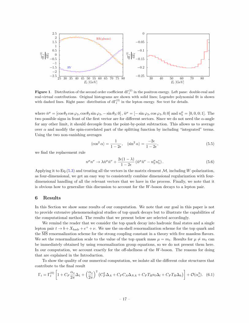
Figure 1. Distribution of the second order coefficient dΓ(2)t in the positron energy. Left pane: double-real and

real-virtual contributions. Original histograms are shown with solid lines; Legendre polynomial fit is shown

with dashed lines. Right pane: distribution of dΓ(2)t in the lepton energy. See text for details.

where nµ = [cos θ3 cosϕ3, cos θ3 sinϕ3,− sin θ3; 0] , nµ = [− sinϕ3, cosϕ3, 0; 0] and nµ5 = [0, 0, 0; 1]. The

two possible signs in front of the first vector are for different sectors. Since we do not need the α-angle

for any other limit, it should decouple from the point-by-point subtraction. This allows us to average

over α and modify the spin-correlated part of the splitting function by including “integrated” terms.

Using the two non-vanishing averages

〈cos2 α〉 =1

1− 2ε, 〈sin2 α〉 =

−2ε

1− 2ε, (5.5)

we find the replacement rule

nµnν → λnµnν +2ε(1− λ)

1− 2ε(nµnν − nµ5nν5) . (5.6)

Applying it to Eq.(5.3) and treating all the vectors in the matrix elementM, including W -polarization,

as four-dimensional, we get an easy way to consistently combine dimensional regularization with four-

dimensional handling of all the relevant vectors that we have in the process. Finally, we note that it

is obvious how to generalize this discussion to account for the W -boson decays to a lepton pair.

6 Results

In this Section we show some results of our computation. We note that our goal in this paper is not

to provide extensive phenomenological studies of top quark decays but to illustrate the capabilities of

the computational method. The results that we present below are selected accordingly.

We remind the reader that we consider the top quark decay into hadronic final states and a single

lepton pair t→ b+Xhadr + e+ + ν. We use the on-shell renormalization scheme for the top quark and

the MS renormalization scheme for the strong coupling constant in a theory with five massless flavors.

We set the renormalization scale to the value of the top quark mass µ = mt. Results for µ 6= mt can

be immediately obtained by using renormalization group equations, so we do not present them here.

In our computation, we account exactly for the off-shellness of the W -boson. The reasons for doing

that are explained in the Introduction.

To show the quality of our numerical computation, we isolate all the different color structures that

contribute to the final result

Γt = Γ(0)t

[1 + CF

αs2π

∆1 +(αs

2π

)2 (C2F∆A + CFCA∆NA + CFTRnl∆l + CFTR∆h

)]+O(α3

s). (6.1)

– 17 –

The different contributions to second order corrections were computed in a number of papers a decade

ago for top quark decays to an on-shell W boson. Since ∆A,NA,l,h, as defined in Eq.(6.1), are relative

corrections, we expect that the importance of the W -off-shellness effect is reduced. We use the analytic

computation of Refs. [20, 21] performed as an expansion in mW /mt, to infer numerical values for the

coefficients. We employ the input parameters mt = 172.85 GeV and mW = 80.419 GeV to obtain

[20, 21]

CFTR∆l = 7.978, CFTR∆h = −0.1166, C2F∆A = 23.939, CFCA∆NA = −134.24. (6.2)

We compare these results of the analytic computation [20, 21] with our numerical results. We find5

CFTR∆numl = 7.970(6), CFTR∆num

h = −0.11662(1),

C2F∆num

A = 24.38(25), CFCA∆numNA = −133.6(4),

(6.3)

where integration errors are explicitly shown. By comparing Eq.(6.2) and Eq.(6.3), we find good

agreement between results of analytic and numerical computations. The level of agreement is rather

striking since there are large cancellations between various contributions to the NNLO final result. To

illustrate this point, we show individual contributions to the abelian coefficient C2F∆num

A with their

integration errors. They read

C2F∆A,RR = −127.12(23), C2

F∆A,RV = 60.24(6), C2F∆A,VV = 83.0154(5),

C2F∆A,ren = 16.513(12), C2

F∆A,qq = −8.227(2),

C2F∆A = C2

F∆A,RR + C2F∆A,RV + C2

F∆A,VV + C2F∆A,ren + C2

F∆A,qq = 24.38(25),

where we include double-real (RR), real-virtual (RV), two-loop virtual (VV), renormalization and

quark-pair corrections. Comparing individual contributions with the final result for ∆A, we observe

very significant cancellations. It is therefore quite remarkable that we can maintain O(1%) error on

the NNLO coefficient.

We now turn to the discussion of kinematic distributions. To facilitate this discussion, we write

the differential decay rate as

dΓt = dΓ(0)t +

(αs2π

)dΓ

(1)t +

(αs2π

)2

dΓ(2)t +O(α3

s), (6.4)

and plot dΓ(2)t /dx in Figs. 1, 2 for various observables x. In particular, in Fig. 1 we show dΓ

(2)t /dEl,

where El is the positron energy. The final result for NNLO QCD corrections arises as a result of

large cancellations between various contributions, most notably the double-real and the real-virtual

ones. To illustrate this point, we show these contributions individually in the left pane and the

sum of all contributions to dΓ(2)t /dEl in the right pane. We note that at smaller values of El the

final result is about ten times smaller than double-real and real-virtual contributions separately. At

this level of cancellations, bin-bin fluctuations that are barely seen for double-real and real-virtual

contributions individually (left pane in Fig. 1) become a serious issue. To overcome it, we choose to fit

individual contributions to the sum of Legendre polynomials and then add fitted results rather than

original histograms. Upon doing that, we find that our final result for dΓ(2)t /dEl exhibits a re-assuring

pattern. Suppose, we account for NL Legendre polynomials in the fit. If NL is too small, we find

that the resulting dΓ(2)t /dEl is not stable against including more polynomials into the fit. If NL is too

5 All numerical results presented in this Section are obtained using the adaptive Monte-Carlo algorithm VEGAS [58]

as implemented in the CUBA library [59].

– 18 –

−0.11

−0.1

−0.09

−0.08

−0.07

−0.06

30 50 70 90 110 130

dΓ(2)

t

dm

lj

mlj [GeV]

−8

−7

−6

−5

−4

−3

−2

−1

0

1−1 −0.58 −0.16 0.26 0.68

dΓ(2)

t

dcosθ l

[GeV

]

cos θl

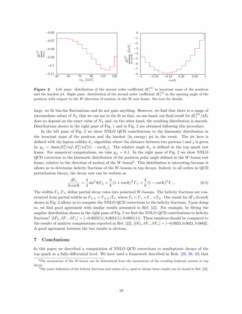
Figure 2. Left pane: distribution of the second order coefficient dΓ(2)t in invariant mass of the positron

and the hardest jet. Right pane: distribution of the second order coefficient dΓ(2)t in the opening angle of the

positron with respect to the W -direction of motion, in the W -rest frame. See text for details.

large, we fit bin-bin fluctuations and do not gain anything. However, we find that there is a range of

intermediate values of NL that we can use in the fit so that, on one hand, our final result for dΓ(2)t /dEl

does no depend on the exact value of NL and, on the other hand, the resulting distribution is smooth.

Distributions shown in the right pane of Fig. 1 and in Fig. 2 are obtained following this procedure.

In the left pane of Fig. 2 we show NNLO QCD contributions to the kinematic distribution in

the invariant mass of the positron and the hardest (in energy) jet in the event. The jet here is

defined with the lepton collider k⊥-algorithm where the distance between two partons i and j is given

by yij = 2min(E2i /m

2t , E

2j /m

2t )(1 − cos θij). The relative angle θij is defined in the top quark rest

frame. For numerical computations, we take yij = 0.1. In the right pane of Fig. 2 we show NNLO

QCD correction to the kinematic distribution of the positron polar angle defined in the W -boson rest

frame, relative to the direction of motion of the W -boson6. This distribution is interesting because it

allows us to determine helicity fractions of the W -bosons in top decays. Indeed, to all orders in QCD

perturbation theory, the decay rate can be written as

dΓtd cos θl

=3

4sin2 θlΓL +

3

8(1 + cos θl)

2Γ+ +

3

8(1− cos θl)

2Γ−. (6.5)

The widths ΓL,Γ± define partial decay rates into polarized W -bosons. The helicity fractions are con-

structed from partial widths as F±,L = Γ±,L/Γt, where Γt = Γ+ +Γ−+ΓL. Our result for dΓt/d cos θlshown in Fig. 2 allows us to compute the NNLO QCD corrections to the helicity fractions. Upon doing

so, we find good agreement with similar results presented in Ref. [22]. For example, by fitting the

angular distribution shown in the right pane of Fig. 2 we find the NNLO QCD contributions to helicity

fractions7 [δFL, δF−, δF+] = [−0.0022(1), 0.0021(1), 0.0001(1)]. These numbers should be compared to

the results of analytic computations reported in Ref. [22], [δFL, δF−, δF+] = [−0.0023, 0.0021, 0.0002].

A good agreement between the two results is obvious.

7 Conclusions

In this paper we described a computation of NNLO QCD corrections to semileptonic decays of the

top quark at a fully-differential level. We have used a framework described in Refs. [29, 30, 35] that

6The momentum of the W -boson can be determined from the momentum of the recoiling hadronic system in top

decay.7The exact definition of the helicity fractions and values of αs used to obtain these results can be found in Ref. [22].

– 19 –

combines sector-decomposition and Frixione-Kunszt-Signer phase-space partitioning to disentangle

overlapping kinematic regions that may lead to soft and collinear singularities. We have shown that

this technique works in the same way as parton level Monte Carlo integrators at next-to-leading order,

so that weighted events can be generated and a variety of kinematic distributions can be computed in

a single run of the program.

There is a number of phenomenological applications of the calculation reported in this paper that

we envision. Eventually, it will be combined with the perturbative QCD description of the top quark

production process, to provide NNLO QCD results for pp → tt → W+W−bb in the narrow width

approximation. It can also be used to investigate the dependence of various observables studied in

top quark decays, for example the helicity fractions, on kinematic cuts applied to top quark decay

products. A minor modification of our calculation turns it into a NNLO QCD result for the most

important contribution to the single top production process in hadron collisions. Finally, as explained

in the Introduction, our calculation can be adapted to explore the impact of NNLO QCD corrections to

inclusive charmless semileptonic decays of b-quarks on the determination of the CKM matrix element

|Vub|. We plan to return to these applications in the near future.

Acknowledgments We are grateful to T. Hahn for advises on CUBA and to F. Tramontano

for answering questions about Ref. [6]. We would like to thank J. Gao, C. S. Li and H. X. Zhu for

pointing out an error in one of the plots of the original version of this manuscript. The research of

F.C. and K.M. is supported by US NSF under grant PHY-1214000. The research of K.M. and M.B. is

partially supported by Karlsruhe Institute of Technology through a grant provided by its Distinguished

Researcher Fellowship Program. The research of M.B. is partially supported by the DFG through the

SFB/TR 9 “Computational Particle Physics”. Calculations described in this paper were performed at

the Homewood High Performance Computer Cluster at Johns Hopkins University.

A Tree-level amplitudes

In this Appendix we collect formulas for helicity amplitudes for top quark decay processes t → b +

ngg + e+ + ν, for ng ≤ 2. We note that we prefer to use helicity amplitudes for reasons of speed

and efficiency of the computation. While for top quark decay this is not a critical issue – the number

of diagrams is sufficiently small even at NNLO – it becomes essential if one considers applicability

of similar techniques to more complicated processes. Some amplitudes that we present below have

already appeared in the literature [7] while others are new.

To deal with the massive top quark, we follow the standard procedure that is based on the

decomposition of a time-like four-momentum into a sum of two light-like four-momenta [60]. To

accomplish this, we choose an arbitrary light-like momentum η and write

pt = p1 +m2t

sptηη, (A.1)

where sij = 2pi · pj . We note that p21 = 0 by construction. We can now write the top quark spinor as

u−(pt) = ( 6 pt +mt)|η〉1

〈1η〉 = |1] + |η〉 mt

〈1η〉 ,

u+(pt) = (6 pt +mt)|η]1

[1η]= |1〉+ |η]

mt

[1η],

(A.2)

– 20 –

where we use the standard notation for spinor-helicity variables. In particular, for p2i = 0, |i〉 = |pi〉 =

u+(pi) and |i] = |pi] = u−(pi). It is convenient to choose the auxiliary momentum η to be the positron

momentum p6 to compute helicity amplitudes.

We now present results for helicity amplitudes starting from the tree-level process t(pt)→ b(p2) +

ν(p5) + e+(p6). We introduce the Breit-Wigner denominator DW (p2W ) = (p2

W −m2W + imWΓW )−1

and write the amplitude as

Aht(pt, p2; p5, p6) = g2WDW (s56)δi1i2Aht(1, 2; 5, 6) ≡ Fδi1i2Aht(1, 2; 5, 6). (A.3)

The amplitude Aht(1, 2; 5, 6) is the color-stripped amplitude and it only depends on the helicity of the

top quark ht since helicities of all massless fermions are fixed thanks to the left-handed nature of the

weak current. We find

A+(1, 2; 5, 6) = 0, A−(1, 2; 5, 6) = 〈25〉 [61] . (A.4)

In this case the sum over colors and helicities is trivial; the amplitude squared reads∑col,hel

Aht(pt, p2; p5, p6) = |F|2Nc |A−(1, 2; 5, 6)|2 . (A.5)

Next, we consider amplitudes for the process t(pt)→ b(p2) + g(p3) + ν(p5) + e+(p6). We write it

as

Ahthg (pt, p2, p3; p5, p6) = gsFT a3i2i1Ahthg (1, 2, 3; 5, 6), (A.6)

where T a is an SU(3) color matrix normalized as Tr(T aT b) = δab and ht,g are helicities of the top

quark and of the gluon, respectively. We obtain the following results for the color-stripped helicity

amplitudes

A−−(1, 2, 3; 5, 6) = − [61]〈3|p56|2]〈25〉〈3|pt|3][32]

− [61]〈35〉[32]

,

A−+(1, 2, 3; 5, 6) = − [61]〈2|p56|3]〈25〉〈3|pt|3]〈23〉 − [31][63]〈2|5〉

〈3|pt|3],

A++(1, 2, 3; 5, 6) = −mt〈25〉[63]

2

[61] 〈3|pt|3],

A+− = 0,

(A.7)

where p56 = p5 + p6. The sum over colors is trivial also in this case. We find∑col

|A|2 = |F|2g2s(N2

c − 1)|A|2 = 2NcCF |F|2g2s |A|2. (A.8)

The last set of tree amplitudes that we require for our calculation are the ones that describe the

process with two gluons in the final state t(pt)→ b(p2) + g(p3) + g(p4) + ν(p5) + e+(p6). We write

Ahthg3hg4 (pt, p2, p3, p4; p5, p6) = Fg2s

∑σ

(T aσ3 · T aσ4 )i2i1 Ahthgσ3 hgσ4 (1, 2, σ(3), σ(4); 5, 6), (A.9)

– 21 –

where σ denotes two permutations of the gluons g3, g4. The color-stripped helicity amplitudes are

computed to be

A−−− =[61]〈25〉[2|ptp34|2]

st34[32][42][43]− [61]〈4|p56|2]〈25〉〈3|pt|2]

st34[32][42][3|pt|3〉

+[61]〈45〉〈3|pt|2]

[32][42][3|pt|3〉− [61]〈45〉

[32][43]− [61]〈35〉

[42][43],

A−−+ = 〈25〉(

[61]

[43]〈34〉

(− [42]〈23〉2s234〈2|4〉

+〈3|pt|4]2

st34〈3|pt|3]+〈2|3〉〈3|pt|4]

〈3|pt|3]〈2|4〉

)+

[4|1][6|4]〈3|pt|4]

st34[4|3]〈3|pt|3]

)− [6|1]〈2|3〉2〈3|5〉

s234〈2|4〉〈3|4〉,

A−+− =[61]〈25〉[43]〈34〉

([32]〈4|pt|3]

[42]〈3|pt|3]− [32]2〈24〉

s234[42]+〈4|pt|3]2

st34〈3|pt|3]

)+

+[61]〈45〉[42]〈34〉

([32]〈24〉s234

− 〈4|pt|3]

〈3|pt|3]

)+

[63][31]〈25〉[43]〈3|pt|3]

(−〈4|pt|3]

st34− [32]

[42]

)+

[31][63]〈45〉[42]〈3|pt|3]

,

A−++ =〈25〉st34

([61]〈2|p56|4]〈4|pt|3]

〈24〉〈34〉〈3|pt|3]− [31][63]〈2|p56|4]

〈24〉〈3|pt|3]+

[61]〈2|pt|3]

〈24〉〈34〉 +

+[41][64]〈4|pt|3]

〈34〉〈3|pt|3]− [31][43][64]

〈3|pt|3]+

[31][63]〈23〉〈24〉〈34〉 +

2[31][64]

〈34〉

),

and

A+−− = 0,

A+−+ = mt[64]2〈25〉〈3|pt|4]

st34[43][61]〈3|pt|3],

A++− = mt[63]2

[61]〈3|pt|3]

(−〈25〉〈4|pt|3]

st34[43]+〈45〉[42]

− [32]〈25〉[42][43]

),

A+++ = mt〈25〉

〈34〉〈3|pt|3]

([43]〈1|p34|6]

st34+

[63]〈2|p34|6]

[61]〈24〉

),

(A.10)

with st34 = s34 − s3t − s4t. The color-summed amplitude now reads

∑col

|A|2 = 4Nc|F|2g4sCF

[CF(|A(1, 2, 3, 4; 5, 6)|2 + |A(1, 2, 4, 3; 5, 6)|2

)+

+

(CF −

CA2

)2Re [A(1, 2, 3, 4; 5, 6)A∗(1, 2, 4, 3; 5, 6)]

]. (A.11)

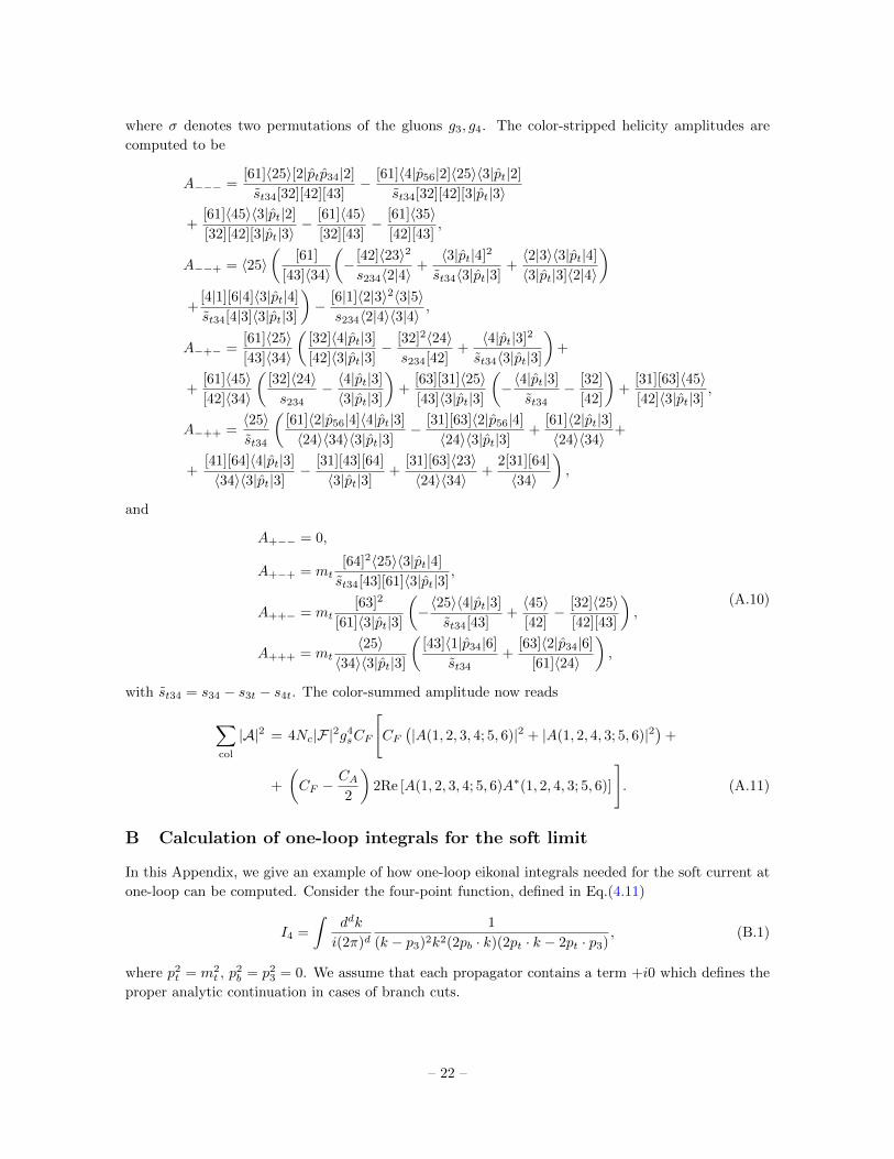
B Calculation of one-loop integrals for the soft limit

In this Appendix, we give an example of how one-loop eikonal integrals needed for the soft current at

one-loop can be computed. Consider the four-point function, defined in Eq.(4.11)

I4 =

∫ddk

i(2π)d1

(k − p3)2k2(2pb · k)(2pt · k − 2pt · p3), (B.1)

where p2t = m2

t , p2b = p2

3 = 0. We assume that each propagator contains a term +i0 which defines the

proper analytic continuation in cases of branch cuts.

– 22 –

To compute I4, we first combine k2 and (k − p3)2 using Feynman parameters

1

k2(k − p3)2=

1∫0

dx

[(k − xp3)2]2. (B.2)

Next, we exponentiate the eikonal quark propagators introducing the integrals over “proper time”

1

(2pt · k − 2pt · p3 + i0)(2k · pb + i0)= −

∞∫0

dτ1dτ2ei2k·pbτ1+i(2pt·k−2pt·p3)τ2 . (B.3)

We now combine Eqs.(B.2, B.3) and shift the loop momentum k → k + p3x. The resulting integral

becomes

I4 = i

∞∫0

dτ1dτ2

1∫0

dxei(−2pt·p3(1−x)τ2+2p3·pbxτ1)

∫ddk

(2π)d1

[k2]2eik(2ptτ2+2pbτ1). (B.4)

The integral over k is easily evaluated∫ddk

(2π)d1

[k2]2eik(2ptτ2+2pbτ1) =

i1+2εΓ(−ε)(4π)d/2

[m2t τ

22 + 2pt · pbτ2τ1]ε. (B.5)

To proceed further, we change variables τ1 = τ2ξ, 0 ≤ ξ ≤ ∞ and integrate over τ2 and x. We obtain

I4 =− Γ(−ε)Γ(1 + 2ε)

(4π)d/2

∞∫0

dξ (m2t + 2pt · pbξ)ε

(2pt · p3 + 2pb · p3ξ)

(e2πiε

(2pb · p3ξ)1+2ε+

1

(2pt · p3)1+2ε

). (B.6)

The final integration over ξ is easy to perform in terms of hypergeometric functions. The result is

shown in Eq.(4.12).

References

[1] M. Jezabek and J.H. Kuhn, Nucl. Phys. B314, 1 (1989).

[2] A. Czarnecki, Phys. Lett. B252, 467 (1990).

[3] C.S. Li, R.J. Oakes and T.C. Yuan, Phys. Rev. D43, 3759 (1991).

[4] A. Denner and T.Sack, Nucl. Phys. B358, 46 (1991); G. Eliam, R. Mendel, R. Mingeron and A. Soni,

Phys. Rev. Lett. 66, 3105 (1991).

[5] J. Campbell, R. K. Ellis and F. Tramontano, Phys. Rev. D70, 094012 (2004).

[6] J. M. Campbell and F. Tramontano, Nucl. Phys. B726, 109 (2005) [hep-ph/0506289].

[7] J. M. Campbell and R. K. Ellis, arXiv:1204.1513 [hep-ph].

[8] K. Melnikov and M. Schulze, JHEP 0908, 049 (2009) [arXiv:0907.3090 [hep-ph]].

[9] W. Bernreuther and Z. -G. Si, Nucl. Phys. B 837, 90 (2010) [arXiv:1003.3926 [hep-ph]].

[10] K. Melnikov, M. Schulze and A. Scharf, Phys. Rev. D 83, 074013 (2011) [arXiv:1102.1967 [hep-ph]].

[11] K. Melnikov, A. Scharf and M. Schulze, Phys. Rev. D 85, 054002 (2012) [arXiv:1111.4991 [hep-ph]].

– 23 –

[12] P. Baernreuther, M. Czakon and A. Mitov, Phys. Rev. Lett. 109, 132001 (2012) [arXiv:1204.5201

[hep-ph]].

[13] M. Czakon and A. Mitov, JHEP 1212, 054 (2012) [arXiv:1207.0236 [hep-ph]].

[14] M. Czakon and A. Mitov, arXiv:1210.6832 [hep-ph].

[15] A. Denner, S. Dittmaier, S. Kallweit and S. Pozzorini, Phys. Rev. Lett. 106, 052001 (2011)

[arXiv:1012.3975 [hep-ph]].

[16] A. Denner, S. Dittmaier, S. Kallweit and S. Pozzorini, JHEP 1210, 110 (2012) [arXiv:1207.5018

[hep-ph]].

[17] See contirbution by A. Denner, S. Dittmaier, S. Kallweit, S. Pozzorini and M. Schulze to J. Alcaraz

Maestre et al. [SM AND NLO MULTILEG and SM MC Working Groups Collaboration],

arXiv:1203.6803 [hep-ph], page 55.

[18] A. Czarnecki and K. Melnikov, Nucl. Phys. B544, 520 (1999).

[19] K. G. Chetyrkin, R. Harlander, T. Seidenstcker and M. Steinhauser, Phys. Rev. D60, 114015 (1999).

[20] I.R. Blokland, A. Czarnecki, M. Slusarczyk and F. Tkachov, Phys. Rev. Lett. 93, 062001 (2004).

[21] I. Blokland, A. Czarnecki, M. Slusarczyk, F. Tkachov, Phys. Rev. D71, 054004 (2005) [Erratum-ibid.

D79, 019901 (2009) ].

[22] A. Czarnecki, J. G. Korner and J.H. Piclum, Phys. Rev. D81, 111503 (2010).

[23] J. Gao, C. S. Li and H. X. Zhu, arXiv:1210.2808 [hep-ph].

[24] C.W. Bauer, S. Fleming, D. Pirjol and I.W. Stewar, Phys. Rev. D63, 114020 (2001); C.W. Bauer,

D. Pirjol and I.W. Stewar, Phys. Rev. D65, 054022 (2002); M. Beneke, A.P. Chapovsky, M. Diehl and

T. Feldmann, Nucl. Phys. B 643, 431 (2002).

[25] C.W. Bauer, Z. Ligeti and M.E. Luke, Phys. Lett. B479, 395 (2000).

[26] C.W. Bauer, Z. Ligeti and M.E. Luke, Phys. Rev. D64, 113004 (2001).

[27] P. Gambino, G. Ossola, N. Uraltsev, JHEP 0509, 010 (2005).

[28] P. Gambino, P. Giordano, G. Ossola and N. Uraltsev, JHEP 0710, 058 (2007).

[29] M. Czakon, Phys. Lett. B693, 259 (2010).

[30] M. Czakon, Nucl. Phys. B849, 250 (2011).

[31] T. Binoth and G. Heinrich, Nucl. Phys. B585, 741 (2000).

[32] T. Binoth and G. Heinrich, Nucl. Phys. B693, 138 (2004).

[33] C. Anastasiou, K. Melnikov and F. Petriello, Phys. Rev. D69, 076010 (2004).

[34] S. Frixione, Z. Kunszt and A. Signer, Nucl. Phys. B 467, 399 (1996) [hep-ph/9512328].

[35] R. Boughezal, K. Melnikov and F. Petriello, Phys. Rev. D 85, 034025 (2012) [arXiv:1111.7041 [hep-ph]].

[36] L. J. Dixon, In Boulder 1995, QCD and beyond 539-582 [hep-ph/9601359].

[37] R. Bonciani and A. Ferroglia, JHEP 0811, 065 (2008).

[38] G. Bell, Nucl. Phys. B812, 264 (2009).

[39] H. Astarian, C. Greub and B. Pecjak, Phys. Rev. D78, 114028 (2008).

[40] M. Beneke, T. Huber and X.-Q. Li, Nucl. Phys. B811, 77 (2009).

[41] T. Huber, JHEP 0903, 024 (2009) [arXiv:0901.2133 [hep-ph]].

– 24 –

[42] S. Catani and M. Grazzini, Phys. Rev. Lett. 98, 222002 (2007) [hep-ph/0703012].

[43] S. Weinzierl, JHEP 0303, 062 (2003) [hep-ph/0302180].

[44] G. Somogyi, P. Bolzoni and Z. Trocsanyi, Nucl. Phys. Proc. Suppl. 205-206, 42 (2010) and references

therein.

[45] M. Grazzini, JHEP 02, 043 (2008); S. Catani, L. Cieri, G. Ferrera, D. de Florian, and M. Grazzini,

Phys. Rev. Lett. 103, 082001 (2009); G. Ferrera, M. Grazzini, and F. Tramontano, Phys. Rev. Lett.

107, 152003 (2011); S. Catani, L. Cieri, D. de Florian, G. Ferrera, and M. Grazzini, Phys. Rev. Lett.

108, 072001 (2012); C. Anastasiou, K. Melnikov, and F. Petriello, Phys. Rev. Lett. 93, 262002 (2004);

K. Melnikov and F. Petriello, Phys. Rev. D 74, 114017 (2006); A. Gehrmann-De Ridder, T. Gehrmann,

E. W. N. Glover, and G. Heinrich, JHEP 12, 094 (2007); A. Gehrmann-De Ridder, T. Gehrmann,

E. W. N. Glover, and G. Heinrich, Phys. Rev. Lett. 100, 172001 (2008); S. Weinzierl, Phys. Rev. Lett.

101, 162001 (2008) 162001.

[46] A. Gehrmann-De Ridder, T. Gehrmann and E. W. N. Glover, JHEP 0509, 056 (2005) [hep-ph/0505111].

[47] A. Daleo, T. Gehrmann and D. Maitre, JHEP 0704, 016 (2007) [hep-ph/0612257].

[48] C. Anastasiou, F. Herzog and A. Lazopoulos, JHEP 1103, 038 (2011) [arXiv:1011.4867 [hep-ph]].

[49] A. Gehrmann-De Ridder, T. Gehrmann and M. Ritzmann, JHEP 1210, 047 (2012) [arXiv:1207.5779

[hep-ph]].

[50] D. A. Kosower, P. Uwer, Nucl. Phys. B563, 477 (1999).

[51] J. M. Campbell and R.K. Ellis, Phys. Rev. D 62, 114012 (2000). The MCFM program is publicly

available from http://mcfm.fnal.gov.

[52] R. K. Ellis and G. Zanderighi, JHEP 0802, 002 (2008) [arXiv:0712.1851 [hep-ph]].

[53] A. Denner, Fortschr. Phys. 41, 307 (1993) [arXiv:0709.1075].

[54] R. Gavin, Y. Li, F. Petriello and S. Quackenbush, Comput. Phys. Commun. 182, 2388 (2011)

[arXiv:1011.3540 [hep-ph]].

[55] S. Catani and M. Grazzini, Nucl. Phys. B 570, 287 (2000) [hep-ph/9908523].

[56] S. Catani and M. Grazzini, Nucl. Phys. B 591, 435 (2000).

[57] I. Bierenbaum, M. Czakon and A. Mitov, Nucl. Phys. B 856, 228 (2012) [arXiv:1107.4384 [hep-ph]].

[58] G.P. Lepage, Cornell preprint CLNS-80/447

[59] T. Hahn, Comput.Phys.Commun. 168, 78 (2005).

[60] R. Kleiss and J. Stirling, Nucl. Phys. B262, 235 (1985).

– 25 –