Polymorphic Intersection Type Assignment for RewriteSystems with Abstraction and β-rule∗

Steffen van Bakel1, Franco Barbanera 2, and Maribel Fernandez 3

1 Department of Computing, Imperial College,180 Queen’s Gate, London SW7 2BZ, U.K.

2 Dipartimento di Matematica e Informatica, Universita degli Studi di Catania,Viale A. Doria 6, 95125 Catania, Italia.

3 DI - LIENS, Ecole Normale Superieure / CNRS,45, rue d’Ulm, 75005 Paris, France.

svb@doc.ic.ac.uk, barba@dipmat.unict.it, maribel@di.ens.fr

Abstract

We define two type assignment systems for first-order rewriting extended with application,λ-abstraction, and β-reduction, using a combination of intersection types and second-orderpolymorphic types. The first system is the general one, for which we prove subject reduction,and strong normalisation of typeable terms. The second is a decidable subsystem of the first,by restricting to rank 2 (intersection and quantified) types. For this system we define, usingan extended notion of unification, a notion of principal typing which is more general thanml’s principal type property, since also the types for the free variables of terms are inferred.

Introduction

Since the first investigations on combinations of Lambda Calculus (lc) and Term RewritingSystems (trs) [13, 19, 14, 26], this topic has drawn attention from the theoretical computerscience community. At first, the area of programming language design was consider to bethe typical field on which the theoretical results for combinations of the two computationalparadigms could better exploit their potentialities. Later on, the evolution of interactiveproof development tools with inductive types, and theorem provers in general, disclosed anumber of possible applications.

Apart from the practical outcome, most of the theoretical investigations in this particularfield have shown that type disciplines provide an optimal environment in which rewriterules and β-reduction can interact without loss of their useful properties [14, 15, 26, 9, 10, 7].Type disciplines come in two main flavours: explicitly typed (also called a la Church) and typeinference systems (a la Curry). Systems based on the latter sort of type discipline are of greatinterest from the point of view of programming language design. In fact, they save theprogrammer from specifying a type for each variable (i.e. no type annotation is required).Most of the results about combinations of lc and trs, however, concern systems which areexplicitly typed.

In the context of the lc alone, type inference disciplines have been widely studied, in par-ticular with intersection types, and some work has also been done for trs alone, more pre-cisely, for Curryfied trs (Cutrs) [8] which are first-order trs with application, that correspondto the trs underlying the programming language Clean [34]. The interactions between lcand trs for type systems a la Curry, instead, has not been extensively investigated. They

∗ Partially supported by NATO Collaborative Research Grant CRG 970285 ‘Extended Rewriting and Types’.

1

were first studied in [7], where Cutrs extended with λ-abstraction and β-reduction were de-fined, together with a notion of intersection type assignment for both the lc and the trsfragments. In this paper we carry on this study by taking explicit polymorphism into account,namely the possibility, from the programming language point of view, of using the sameprogram with arguments of different types.

We take into account also another important feature of type systems for programminglanguages: the notion of principal type, that is, a type from which all the other types of a termcan be derived. As a matter of fact we consider an even stronger property than principaltypes: the principal typing property. This means that any typing judgement for a term can beobtained from the principal one, that is, not only the type but also the basis (containing thetype assumptions for the free variables) is obtained. The pragmatic value of this propertyis demonstrated in [25], where it is shown that, unlike principal types, principal typingsprovide support for separate compilation, incremental type inference, and for accurate typeerror messages.

The type system of ml is polymorphic and has principal types, but its polymorphism islimited (some programs that arise naturally cannot be typed), and it does not have principaltypings (see [17, 25]). System F [23] provides a much more general notion of polymorphism,but lacks principal types, and type inference is undecidable in general (although it is decid-able for some subsystems, in particular if we consider types of rank 2 [27]). Intersection typesystems [12] are somewhere in the middle with respect to polymorphism, and have principaltypings. But type assignment is again undecidable; decidability is recovered if we restrictourselves to intersection types of finite rank [29].

In [24], a system for lc combining intersection types and System F was presented, whichhas principal typings (see [32]). In this paper we extend the approach of that system to acombination of lc and Cutrs. In other words, we extend the type system of [7] further, adding‘∀ ’ as an extra type-constructor (i.e. explicit polymorphism). Although extending the set oftypes by adding ‘∀ ’ does not extend the expressivity of the system in terms of typeableterms, the set of assignable types increases, and types can better express the behaviour ofterms (see [16]). The resulting system has the expected properties: Subject Reduction, andStrong Normalization when the rewrite rules use a limited form of recursion (inspired by theGeneral Schema of Jouannaud and Okada [26]). The proof of the latter follows the method ofTait-Girard’s reducibility candidates, extended in order to take the presence of (higher-order)algebraic rewriting into account.

In view of the above results, two questions arise naturally:

i) Is the Rank 2 combination of System F and the Intersection System also decidable?ii) Does it have the principal typing property?

We answer these questions in the affirmative. The restriction to types of rank 2 of thecombined system of polymorphic and intersection types is decidable. This restricted systemcan be seen as a combination of the systems considered in [6] and [27]. The combinationis two-fold: not only the type systems of those two papers are combined (resp. intersectionand polymorphic types of rank 2), but also their calculi are combined (resp. Cutrs and lc).In our Rank 2 system each typeable term has a principal typing. This is the case also in theRank 2 intersection system of [6], but not in the Rank 2 polymorphic system of [27]. Forthe latter, a type inference algorithm of the same complexity of that of ml was given in [28],where the problems that occur due to the lack of principal types are discussed in detail. OurRank 2 system generalizes also Jim’s system P2 [25], which is a combination of ml-types andRank 2 intersection types. Having Rank 2 quantified types in the system allows us to typefor instance the constant runST used in [31], which cannot be typed in P2.

This paper is organised as follows: In Section 1 we define trs with application, λ-abstractionand β-reduction (trs+β), and in Section 2 the type assignment system. Section 3 deals with

2

the strong normalization property for typeable terms, and in Section 4 we prove a confluenceresult. In Section 5 we present the restriction of the general type assignment system to Rank2; finally, Section 6 contains the conclusions.

1 Term Rewriting Systems with β-reduction rule

In this section, we will present a combination of untyped Lambda Calculus with untypedAlgebraic Rewriting, obtained by extending first-order trs with notions of application andabstraction, and a β-reduction rule. We can look at such calculi also as extensions of theCurryfied Term Rewriting Systems (Cutrs) considered in [3, 8], by adding λ-abstraction anda β-reduction rule. We assume the reader to be familiar with lc [11] and refer to [30, 18] forrewrite systems.

Definition 1.1 i) An alphabet or signature Σ consists of a countable, infinite set X of variablesx1, x2, x3, . . . (or x,y,z, x′,y′, . . .), a non-empty set F of function symbols F, G, . . . , each witha fixed arity, and a special binary operator, called application (Ap).

ii) The set T(F,X ) of terms, ranged over by t, is defined by:

t ::= x | F(t1, . . . , tn) | Ap(t1, t2) | λx.t

We will consider terms modulo α-conversion.A context is a term with a hole, and it is denoted as usual by C[].

iii) a) A neutral term is a term not of the form λx.t.b) A lambda term is a term not containing function symbols.c) An algebraic term is a term containing neither λ nor Ap.

The set of free variables of a term t is defined as usual, and denoted by FV(t).

A term-substitution is an operation on terms where terms variables are replaced by terms;as usual for term-substitution in systems with abstraction, we will consider terms moduloα-conversion to avoid name clashes. To denote a term-substitution, we use capital characterslike ‘R’, instead of Greek characters like ‘σ’, which will be used to denote types. Sometimeswe use the notation {x1 �→ t1, . . . , xn �→ tn}. We write tR for the result of applying the term-substitution R to t.

Reductions on T(F,X ) are defined through rewrite rules together with a β-reduction rule.

Definition 1.2 (Reduction) i) A rewrite rule is a pair (l,r) of terms. Often, a rewrite rulewill get a name, e.g. r, and we write l →r r. Three conditions are imposed: l �∈ X , l is analgebraic term, and FV(r) ⊆ FV(l).

ii) A rewrite rule l → r determines a set of rewrites lR → rR for all term-substitutions R. Theleft hand side lR is called a redex, the right hand side rR its contractum. Likewise, forany t and u, the usual notion of β-reduction Ap(λx.t,u) →β t{x �→u} is also a rewrite;Ap(λx.t,u) is called a redex, and t{x �→u} its contractum.

iii) A redex t may be substituted by its contractum t′ inside a context C[]; this gives riseto rewrite steps C[t] → C[t′ ]. Concatenating rewrite steps we have rewrite sequences t0 →t1 → t2 → ·· ·. If t0 → ·· · → tn (n ≥ 0) we also write t0 →∗ tn, and t0 →+ tn if t0 →∗ tn inone step or more.

Definition 1.3 A Term Rewriting System with β-reduction rule (trs+β) is defined by a pair(Σ,R) of an alphabet Σ and a set R of rewrite rules.

3

Note that in contrast with Cutrs, the rewrite rules considered in this paper may containλ-abstractions in the right-hand sides.

We take the view that in a rewrite rule a certain symbol is defined.

Definition 1.4 In a rewrite rule F(t1, . . . , tn)→r r, F is called the defined symbol of r, and r issaid to define F. F is a defined symbol, if there is a rewrite rule that defines F, and Q ∈ F iscalled a constructor if Q is not a defined symbol.

Notice that ‘Ap’ cannot be a defined symbol since it cannot appear in the left-hand side ofa rewrite rule.

Definition 1.5 Let (Σ,R) be a trs+β.

i) A term is in normal form if it contains no redex.ii) A term t is strongly normalisable if all the rewrite sequences starting with t are finite, and

we will write SN (t) if t is strongly normalisable.iii) (Σ,R) is strongly normalising if every term is.iv) (Σ,R) is confluent if for all t such that t →∗ u and t →∗ v, there exists s such that u →∗ s

and v →∗ s.

Example 1.6 The following is a set of rewrite rules that defines the functions append and mapon lists and establishes the associativity of append. The function symbols nil and cons areconstructors.

append(nil, l) → lappend(cons(x, l), l′) → cons(x,append(l, l′))append(append(l, l′), l′′) → append(l,append(l′, l′′))map ( f ,nil) → nilmap ( f ,cons(y, l)) → cons(Ap( f ,y),map ( f , l))

Since variables in trs+β may be substituted by λ-expressions, we obtain the usual func-tional programming paradigm, extended with definitions of operators and data structures.Notice, however, that we obtain more: in functional programs, the set F is divided intofunction symbols and constructors, and, in rewrite rules, function symbols are not allowed toappear in ‘constructor position’ and vice-versa. This does not hold for trs+β: the symbol‘append’ appears in the third rule in both function and constructor position.

2 A Polymorphic Intersection System for trs+β

In this section we define a type assignment system for TRS+β, that can be seen as an ex-tension (by adding ‘∀ ’) of the intersection system presented in [7]. We use polymorphicstrict intersection types, defined over a set of type-variables and sorts (type constants), us-ing arrow, intersection and universal quantifiers. We assume the reader to be familiar withintersection type assignment systems, and refer to [12, 2, 5] for more details.

Several systems can be considered as fragments of our type assignment system:

i) The system of [7]: ∀ -free fragmentii) The system of [8]: λ-free, ∀ -free fragment

iii) The system of [5]: sort-free, ∀ -free, lc-fragmentiv) The type assignment version of System F [23] : intersection-free lc-fragmentv) The system of [32]: sort-free lc-fragment

Indeed, the latter system is not a proper fragment, since we use strict intersection types(i.e. an intersection type cannot be the right-hand side of an arrow type). However this is not

4

an actual difference, since the use of strict intersection types, while simplifying the typingprocedures, does not affect the typing power. Any term typeable in the full intersection typediscipline can be given a strict type and vice-versa [2].

For what concerns System F, its type assignment version can be seen as a fragment of oursystem, but our system is not a pure intersection-extension: we cannot quantify intersectiontypes. Again, this is not a real problem: for any universally quantified intersection type∀α.σ1∩σ2 we have an equivalent type of the form (∀α.σ1)∩(∀α.σ2).

For lc, a type assignment system that combines the intersection system [12] with SystemF has been defined in [24] and its principal type property has been studied in [32]. As far astypes are concerned, the difference between our system and the latter is that we add constanttypes, and use strict intersection types.

2.1 Types

We use strict intersection types over a set V = Φ � A of type-variables, and a set S of sorts.For various reasons (definition of operations on types, definition of unification), we willdistinguish syntactically between (names of) free type-variables (which belong to Φ) and(names of) bound type-variables (in A).

Definition 2.1 (Types) Let Φ = {ϕ0, ϕ1, . . .}, A = {α0,α1, . . .}, and S = {s0, s1, . . .} all be de-numerable sets. Ts, the set of polymorphic strict types, and T , the set of polymorphic strictintersection types, are defined by:

Ts ::= ϕ | s | (T → Ts) | ∀α.Ts[α/ϕ]T ::= (Ts∩ · · · ∩Ts)

To avoid parentheses in the notation of types, ‘→’ is assumed to associate to the right and,as in logic, ‘∩’ binds stronger than ‘→’, which binds stronger than ‘∀ ’; so ρ∩µ→∀α.γ→δstands for ((ρ∩µ)→(∀α.(γ→δ))). Also ∀α.σ is used as abbreviation for ∀α1.∀α2 . . .∀αn.σ,and we assume that each variable is bound at most once in a type (renaming if necessary). Inthe meta-language, we denote by σ[τ/ϕ] (resp. σ[τ/α]) the substitution of the type-variableϕ (resp. α) by τ in σ.

FV(σ), the set of free variables of a type σ is defined as usual (note that by construction,FV(σ) ⊆ Φ). A type is called closed if it contains no free variables, and ground if it containsno variables at all.

Definition 2.2 (Relations on types) The relation ≤ is defined as the least pre-order (i.e.reflexive and transitive relation) on T such that:

∀n ≥ 1,∀1≤ i≤n [σ1∩· · ·∩σn ≤ σi]∀α.σ ≤ σ[τ/α]

σ ≤ ∀α.σ, α not in σ∀n ≥ 1,∀1≤ i≤n [σ ≤ σi] ⇒ σ ≤ σ1∩· · ·∩σn

σ ≤ τ ⇒ ∀α.σ[α/ϕ] ≤ ∀α.τ[α/ϕ]ρ ≤ σ & τ ≤ µ ⇒ σ→τ ≤ ρ→µ

The equivalence relation ∼ on types is defined by: σ ∼ τ ⇐⇒ σ ≤ τ ≤ σ, and we will workwith types modulo ∼ .

Notice that Ts is a proper subset of T , and that σ→(τ∩ρ) is not a type in T (it is notstrict). To obtain a notion of type assignment that is a true extension of System F, the ‘∀ ’type-constructor is allowed to occur on the right of an arrow, so a type like σ→∀α.τ is well-defined. Also note that we cannot quantify intersection types, but we have equivalent typesof the form (∀α.σ1)∩(∀α.σ2).

5

2.2 Type assignment

Before coming to the definition of type assignment, we introduce the notion of basis.

Definition 2.3 (Statement and Basis) i) A statement is an expression of the form t :σ, withσ ∈ T and t ∈ T(F,X ). t is the subject and σ the predicate of t :σ.

ii) A basis B is a partial mapping from variables to types, represented as set of statementswith only distinct variables as subjects.

iii) For bases B1, . . . , Bn, the basis Π{B1, . . . , Bn} is defined by: x:σ1∩· · ·∩σm ∈ Π{B1, . . . , Bn} ifand only if {x:σ1, . . . , x:σm} is the (non-empty) set of all statements about x that occur inB1∪ · · · ∪Bn.

iv) We extend ≤ and ∼ to bases by: B ≤ B′ if and only if for every x:σ′ ∈ B′ there is anx:σ ∈ B such that σ ≤ σ′, and B ∼ B′ if and only if B ≤ B′ ≤ B.

Notice that if n= 0, then Π{B1, . . . , Bn}=∅. We will often write B, x:σ for the basis Π{B,{x:σ}},when x does not occur in B, and write B\x for the basis obtained from B by removing thestatement that has x as subject.

One of the main features of type assignment systems, and intersection systems in partic-ular, is to provide flexibility of typing. This feature seems in contrast with the type rigidityimplicitly possessed by function symbols. They have precise arities and a precise functionalbehaviour, as expressed by the rewriting rules. Developing a type assignment system con-taining function symbols necessarily implies a sort of mediation, for what concerns algebraicterms, between flexibility and rigidity. We achieve this by using an environment providing atype for each function symbol. This approach, however, is not rigid: from the type providedby the environment we can derive many types to be used for different occurrences of thesymbol in a term, all of them ‘consistent’ with that provided type.

Definition 2.4 (Environment) An environment is a mapping E : F → Ts.

2.2.1 Operations on Types

In order to obtain valid instances of the type provided by an environment for a functionsymbol we will use operations which are standard in type systems with intersection types,suitably modified in order to take into account the presence of universal quantifiers. Theseoperations are: substitution, expansion, lifting and closure.

In type systems based on arrow types with type-variables, the operation of substitutiongenerates all valid instances of a given type by replacing types for type variables. In presenceof intersection types, valid instances could also be the result of replacing (sub)types by theintersection of a number of renamed copies of that (sub)type. This is (roughly) what isperformed by the operation of expansion. The operation of lifting, instead, generates instancesof types using the ‘≤’ relation. The last operation we consider, closure, is not present inother type systems with intersection types and has been devised to deal in particular withuniversal quantification.

In the following we shall have to consider the notion of principal typing for a term, thatis the typing from which all the possible typings for the term can be derived. This can beachieved by means of the above discussed operations. This implies that we shall have todefine the above operations not only on types, but also on type derivations (denoted byB �E t :σ, where B is a basis and σ a type). We shall use the same symbols to denote the twoversions of the operations, since the context will always clarify any possible ambiguity.

We will show that all operations are sound in the sense that they preserve typeability,and therefore well-defined when extended to derivations. That is, for any operation op, if

6

B �E t :σ then op(B �E t :σ) is a correct derivation. Of course the variants of the operationson derivations can be composed.

Substitution. We will define substitution as usual in first-order logic, but avoid to go out ofthe set of polymorphic strict intersection types. For example, the replacement of ϕ by τ1∩τ2would transform σ→ϕ into σ→τ1∩τ2, which is not in T . The following definition takes thisfact into account.

Definition 2.5 (Substitution) The substitution (ϕ �→ ρ) : T → T , where ϕ is a type-variablein Φ and ρ ∈ Ts, is defined by:

(ϕ �→ ρ)(ϕ) = ρ(ϕ �→ ρ)(ϕ′) = ϕ′, if ϕ′ �= ϕ(ϕ �→ ρ)(s) = s(ϕ �→ ρ)(α) = α(ϕ �→ ρ)(σ→τ) = (ϕ �→ ρ)(σ) → (ϕ �→ ρ) (τ)

(ϕ �→ ρ)(σ1∩· · ·∩σn) = (ϕ �→ ρ)(σ1)∩ · · · ∩ (ϕ �→ ρ)(σn)(ϕ �→ ρ)(∀α.σ) = ∀α.(ϕ �→ ρ)(σ)

We will use S to denote a generic substitution. Substitutions extend to bases in the naturalway: S(B) = {x:S(ρ) | x:ρ ∈ B}.

For substitutions, the following properties hold:

Property 2.6 Let S be a substitution.

i) If σ ≤ τ, then S(σ) ≤ S(τ).ii) If B ≤ B′, then S(B) ≤ S(B′).

Proof: The second part is a consequence of the first, which is shown by induction on thedefinition of ‘≤’.

Expansion. As mentioned above, the operation of expansion deals with the replacementof a sub-type of a type by an intersection of a number of renamed copies of that sub-type.When a sub-type is expanded, new type variables are generated, and other sub-types mightbe affected (e.g. the expansion of τ in σ→τ might affect also σ: intuitively, each renamedcopy of τ will have an associated copy of σ; see [36] for a detailed explanation). Groundtypes are not affected by expansions since all renamed copies coincide (and σ∩σ ∼ σ).

Two different definitions of expansion appear in the literature for lc, depending on whetherone uses a set of types (see e.g. [36]) or a set of type variables (see e.g. [5]) to compute the setof types affected by the expansion. Our definition is inspired by [36]; the extension to dealwith types containing sorts has already been done in [20], here quantifiers are also takeninto account.

We consider expansions determined by three parameters: the sub-type to be expanded,the number of copies that have to be generated, and the set of types affected by the expan-sion. The third parameter is not present in standard definitions of expansion since it can be“computed”, however we prefer to add it since it simplifies the definition. Of course, we willonly apply an expansion to a type (or to a type derivation) if they are compatible, that is, ifthe third parameter of the expansion contains the corresponding set of affected types.

The types modified by the expansion 〈µ,n, A〉 will be those that end with a type in A. Thenotion of last sub-types in a strict type plays an important role in this operation.

7

Definition 2.7 The set of last sub-types of a type τ ∈ Ts, denoted by last(τ), is defined by:

last(ϕ) = {ϕ}last(s) = {s}last(σ→ρ) = {σ→ρ} ∪ last(ρ)last(∀α.σ) = {∀α.σ} ∪ last(σ[ϕα/α]).

Note that for types of the form ∀α.σ, according to our convention σ is not a well-formedsub-type (free variables must belong to Φ). For this reason we consider a mapping A→Φthat associates to each α a different fresh ϕα ∈ Φ, and rename α in σ, using ϕα. In this waywe can define sub-types of types in T , as usual.

We define now the notion of compatibility between an expansion and a type derivation (itapplies to types as particular case).

Definition 2.8 (Compatibility) We represent a derivation B �E t :σ by a triple 〈B,σ, E〉 whereB is a basis, σ a type, and E the set of types assigned to the function symbols of t in thederivation. An expansion Ex〈µ,n,A〉 (where µ is a type in T , n ≥ 2, and A a finite set of types)is compatible with a derivation represented by 〈B,σ, E〉 if the set A contains the set Lµ(〈B,σ, E〉)defined as follows:

i) Any non-closed strict sub-type of µ is in Lµ(〈B,σ, E〉).ii) Let τ be a non-closed strict (sub)type occurring in 〈B,σ, E〉. If τ′ is a most general

instance (with respect to the universal quantifiers) of τ such that last(τ′)∩Lµ(〈B,σ, E〉) �=∅, then τ′ ∈ Lµ(〈B,σ, E〉).

iii) Any non-closed strict sub-type of τ ∈ Lµ(〈B,σ, E〉) is in Lµ(〈B,σ, E〉).An expansion Ex〈µ,n,A〉 is compatible with a type τ if it is compatible with the triple 〈∅,τ,∅〉.

The definition of expansion, already non-trivial in the intersection system, becomes quiteinvolved in the presence of universal quantifiers. We define it in two steps. First, given theset A of types affected by the expansion, we see which are the variables that will need tobe renamed (for free variables we use substitutions in order to do the renamings, but wealso need to rename bound variables; those renamings are not substitutions according toour definition, but by abuse of terminology we call them substitutions as well). Then, ifthe expansion 〈µ,n, A〉 is compatible with the type τ that we want to expand, we traverse τtop-down searching for maximal sub-types whose last sub-types are in A or have an instance(obtained by replacing bound variables by types) in A. Those sub-types of τ will be replacedby intersections of renamed copies.

Definition 2.9 (Expansion) Let µ be a type in T , n ≥ 2, and A a finite set of types. Theexpansion determined by 〈µ,n, A〉, denoted by Ex〈µ,n,A〉, is defined as follows:

(Renamings) : Let V = {ϕ1, . . . , ϕm} be the set of free type variables occurring in A, and let Si(1≤ i≤n) be the substitution that replaces every ϕj by a fresh variable ϕi

j, and every αj

and ϕαj by αij (actually, Si is just a renaming).

(Expansion of a type) : For any τ ∈ T (without loss of generality we assume that its boundvariables are disjoint with those of µ, A) compatible with the expansion Ex〈µ,n,A〉, thetype Ex〈µ,n,A〉(τ) is obtained out of τ by traversing τ top-down and replacing in τ amaximal non-closed sub-type β such that there exists a most general instance (w.r.t. theuniversal quantifiers) β′ of β with last(β′)∩A �= ∅

a) by S1(β)∩ · · · ∩Sn(β) if β′ = β,b) otherwise by

⋂

1≤j≤p

(S1(β′j)∩ · · · ∩Sn(β′

j)∩∀Si(α).Ex〈µ,n,A〉(ρ[cj/α])[α/cj])

8

if β = ∀α.ρ, β′j (1≤ j≤ p) are all the most general instances of β satisfying the con-

dition, and cj are fresh constants replacing the variables instantiated in the instanceβ′

j of β.

(Expansion of a derivation) : Let B �E t :σ be a type-derivation (represented by the triple 〈B,σ, E〉)compatible with Ex〈µ,n,A〉. The result of the application of the expansion is then a triple:

〈{x:Ex〈µ,n,A〉(ρ) | x:ρ ∈ B},Ex〈µ,n,A〉(σ),{Ex〈µ,n,A〉(ρ) | ρ ∈ E}〉

We will prove below that this triple represents a correct derivation (i.e. expansions aresound on derivations).

Some explanations are in order. The result of an operation of expansion is not uniquebecause it depends on the choice of new variables in part (Renamings) of the definition; but itis unique modulo renaming of variables (and this is sufficient for our purpose). It is alwaysa type in T : we never introduce an intersection at the right-hand side of an arrow type,and never quantify an intersection type (see part (Expansion of a type)). A type might beaffected by an expansion even if its free variables are disjoint with those of the sub-type tobe expanded. The reason is that universally quantified variables represent an infinite set ofterms (their instances), so if one instance is affected, the whole type is affected. If we areapplying an expansion operation to a universally quantified type, some instances may beexpanded (if their last sub-types are in the set of affected types) whereas others are not (iftheir last sub-types are not in this set). In this case the expansion of the universally quantifiedtype will be the intersection of the expansions of each class of instances. Since there is onlya finite set of affected types, the operation is well defined.

Example 2.10 Let γ be (ϕ1→ϕ2)→(ϕ3→ϕ1)→ϕ3→ϕ2, and Ex be the expansion determinedby 〈ϕ1,2,{ϕ1, ϕ3→ϕ1, ϕ3}〉. First, we check that this expansion is compatible with γ: indeed,the set Lϕ1(〈∅,γ,∅〉) = {ϕ1, ϕ3→ϕ1, ϕ3}. Then we compute the set of variables that will berenamed: V = {ϕ1, ϕ3}. The result of the expansion of γ is:

Ex(γ) = ((ϕ11∩ϕ2

1)→ϕ2)→((ϕ13→ϕ1

1)∩(ϕ23→ϕ2

1))→(ϕ13∩ϕ2

3)→ϕ2.

Consider now a type with universal quantifiers and free variables, such as

γ = ∀α2∀α3.(ϕ1→α2)→(α3→ϕ1)→α3→α2,

Then Lϕ1(〈∅,γ,∅〉) = {ϕ1,∀α3.(ϕ1→ϕ1)→(α3→ϕ1)→α3→ϕ1,(ϕ1→ϕ1)→(ϕα3→ϕ1)→ϕα3→ϕ1, ϕ1→ϕ1, ϕα3→ϕ1, ϕα3}

Let Ex be the expansion determined by 〈ϕ1,2,Lϕ1(〈∅,γ,∅〉)〉, which is obviously compat-ible with γ. Then V = {ϕ1} and

Ex(γ) = (∀α3.(ϕ11→ϕ1

1)→(α3→ϕ11)→α3→ϕ1

1)∩ (∀α3.(ϕ21→ϕ2

1)→(α3→ϕ21)→α3→ϕ2

1)∩(∀α2∀α1

3∀α23.(ϕ1

1∩ ϕ21→α2)→((α1

3→ϕ11)∩ (α2

3→ϕ21))→α1

3∩α23→α2).

For an example with sorts, consider γ = (ϕ1→s)→ϕ2, and let Ex be the expansion de-termined by 〈ϕ1→s, 2,{ϕ1→s, ϕ1}〉, which is compatible with γ since Lϕ1→s(〈∅,γ,∅〉) ={ϕ1→s, ϕ1}. Then V = {ϕ1} and Ex(γ) = ((ϕ1

1→s)∩(ϕ21→s))→ϕ2.

If we apply instead the expansion determined by 〈ϕ2,2,Lϕ2(〈∅,γ,∅〉)〉 to γ, where

Lϕ2(〈∅,γ,∅〉) = {ϕ2, (ϕ1→s)→ϕ2, ϕ1→s, ϕ1}, andV = {ϕ2, ϕ1},

we obtain Ex(γ) = ((ϕ11→s)→ϕ1

2)∩((ϕ21→s)→ϕ2

2).

9

For an operation of expansion the following property holds:

Property 2.11 Let Ex= 〈µ,n, A〉 be an expansion compatible with a derivation represented by 〈B,σ, E〉.If x:ρ ∈ B and ρ ≤ σ, then Ex(ρ) ≤ Ex(σ).

Proof: By induction on the definition of ≤.

Lifting. The operation of lifting replaces basis and type by a smaller basis and a larger type,in the sense of ‘≤’ (see [4] for details). This operation allows us to eliminate intersectionsand universal quantifiers, using the ‘≤’ relation. When applying a lifting to a derivationB �E t :σ we will use the pair 〈B,σ〉 to represent the derivation.

Definition 2.12 (Lifting) An operation of lifting is determined by a pair L=<〈B0,τ0〉, 〈B1,τ1〉>such that τ0 ≤ τ1 and B1 ≤ B0, and L(〈B,σ〉) = 〈B′,σ′〉 where

σ′ = τ1, if σ = τ0,σ′ = σ, otherwise

B′ = B1, if B = B0B′ = B, otherwise

A lifting on types is determined by a pair L = 〈τ0,τ1〉 such that τ0 ≤ τ1 and is defined by

L(σ) = τ1, if σ = τ0= σ, otherwise

Closure. The operation of closure introduces quantifiers, taking into account the basis wherea type is used.

Definition 2.13 (Closure) A closure is an operation characterised by a type-variable ϕ. It isdefined by:

Clϕ(〈B,σ〉) = 〈B,∀α.σ[α/ϕ]〉, if ϕ does not appear in B (α is a fresh variable)= 〈B,σ〉, otherwise

It is extended to types by: Clϕ(σ) = (τ), if Clϕ(〈∅,σ〉) = 〈∅,τ〉.

Chains of operations. The set Ch of chains for types is defined as the smallest set containingexpansions, substitutions, liftings, and closures on types, that is closed under composition.

Definition 2.14 (Chains on types) i) A chain is an object [O1, . . . ,On], where each Oi is anoperation of substitution, expansion, lifting, or closure, and

[O1, . . . ,On](σ) = O1(· · · (On(σ)) · · ·).

ii) On chains the operation of concatenation is denoted by ∗ , and:

[O1, . . . ,Oi] ∗ [Oi+1, . . . ,On] = [O1, . . . ,On].

iii) We say that Ch1 = Ch2, if for all σ, Ch1(σ) = Ch2(σ).iv) We extend the notion of compatibility to chains by: Ch is compatible with B �E t :σ if,

for all expansions Ex that occur in Ch (so Ch = Ch1 ∗ [Ex] ∗ Ch2), Ex is compatible withCh1(B �E t :σ).

Notice that, although the operation of substitution seems redundant, in that one couldsimulate substitution via closure and lifting, this is only the case for type variables that donot occur in the basis; to instantiate type-variables that occur in the basis as well, substitutionon types is essential.

10

2.2.2 Type Assignment Rules

We specify how to type terms through the presentation of type assignment rules. To dealwith function symbols we use an environment E and the operations on types defined above:the types assigned to occurrences of function symbols are obtained from the type providedby the environment by making a chain of operations.

Definition 2.15 (Type Assignment Rules) i) Type assignment (with respect to E) is definedby the following natural deduction system in sequent form (where all types displayedare in Ts, except for σ1, . . . ,σn in rule (F) and σ in rules (→E), (→I), and (≤)). Note theuse of a chain of operations in rule (F).

(≤) : (a)B �E x :τ (→I) :

B, x:σ �E t :τ

B �E λx.t :σ→τ(→E) :

B �E t1 :σ→τ B �E t2 :σ

B �E Ap(t1, t2) :τ

(∩I) :B �E t :σ1 · · · B �E t :σn

(n ≥ 1)B �E t :σ1∩· · ·∩σn

(F) :B �E t :σ1 · · · B �E t :σn

(b)B �E F(t1, . . . , tn) :σ

(∀ I) :B �E t : σ

(c)B �E t :∀α.σ[α/ϕ]

(∀E) :B �E t :∀α.σ

B �E t :σ[τ/α]

a) x:σ ∈ B,σ ≤ τ.b) If there exists a chain Ch on types such that σ1→·· ·→σn→σ = Ch(E(F)).c) If ϕ does not occur (i.e. is not free) in B.

ii) If B �E t : σ is derivable in this system, we write B �E t : σ.

As said before, the use of an environment in rule (F) introduces a notion of polymor-phism for our function symbols, which is an extension (with intersection types and generalquantification) of the ml-style of polymorphism. The environment returns the ‘principaltype’ for a function symbol; this symbol can be used with types that are ‘instances’ of itsprincipal type, obtained by applying chains of operations.

Note that the rule (≤) is only defined for variables, and we have a (∀E)-rule for arbitraryterms but not an (∩E)-rule. Indeed, the (∩E)-rule for arbitrary terms can be admitted to thissystem of rules without extending its expressive power. On the other hand, the (∀E)-rulecannot be derived if it is not present in the system. This asymmetry comes from the fact thatour types are strict with respect to ‘∩’, but not with respect to ‘∀ ’.

Example 2.16 We can derive �E λxyz.x(yz) :(ϕ1→ϕ2)→(ϕ3→ϕ1)→ϕ3→ϕ2 as follows, whereB = {x:ϕ1→ϕ2,y:ϕ3→ϕ1,z:ϕ3}:

B �E x : ϕ1→ϕ2

B �E y : ϕ3→ϕ1 B �E z : ϕ3

B �E yz : ϕ1

B �E x(yz) : ϕ2

B\z �E λz.x(yz) : ϕ3→ϕ2

B\y,z �E λyz.x(yz) : (ϕ3→ϕ1)→ϕ3→ϕ2

�E λxyz.x(yz) : (ϕ1→ϕ2)→(ϕ3→ϕ1)→ϕ3→ϕ2

11

and also �E λxyz.x(yz) :∀α3α2.(ϕ1→α2)→(α3→ϕ1)→α3→α2 with a derivation D of the form:

�E λxyz.x(yz) : (ϕ1→ϕ2)→(ϕ3→ϕ1)→ϕ3→ϕ2

�E λxyz.x(yz) :∀α2.(ϕ1→α2)→(ϕ3→ϕ1)→ϕ3→α2

�E λxyz.x(yz) :∀α3α2.(ϕ1→α2)→(α3→ϕ1)→α3→α2

Notice that the sub-derivation for �E λxyz.x(yz) :(ϕ1→ϕ2)→(ϕ3→ϕ1)→ϕ3→ϕ2 in D is ex-actly the one given above, in the sense that no α appears there.

Now, performing the expansions of Example 2.10, we obtain the statements

�E λxyz.x(yz) :((ϕ11∩ϕ2

1)→ϕ2)→((ϕ13→ϕ1

1)∩(ϕ23→ϕ2

1))→(ϕ13∩ϕ2

3)→ϕ2

and�E λxyz.x(yz) :σ1∩σ2∩σ3

where σ1 = ∀α3.(ϕ11→ϕ1

1)→(α3→ϕ11)→α3→ϕ1

1,σ2 = ∀α3.(ϕ2

1→ϕ21)→(α3→ϕ2

1)→α3→ϕ21, and

σ3 = ∀α2∀α13∀α2

3.(ϕ11∩ ϕ2

1→α2)→((α13→ϕ1

1)∩ (α23→ϕ2

1))→α13∩α2

3→α2,which are derived as below (where, in the derivations, we will omit the premisse for rule(≤) (of the shape ‘x:σ ∈ B’) as well as ϕ for lack of space).

Take B = {x : ϕ11→ϕ1

1,y : ϕ3→ϕ1,z:ϕ3}, then, for �E λxyz.x(yz) :σ1:

B �E x : 11→ 1

1

B �E y : 3→ 11 B �E z : 3

B �E yz : 11

B �E x(yz) : 11

B\z �E λz.x(yz) : 3→ 11

B\y,z �E λyz.x(yz) :( 3→ 1)→ 3→ 11

�E λxyz.x(yz) :( 11→ 1

1)→( 3→ 11)→ 3→ 1

1

�E λxyz.x(yz) :∀α3.( 11→ 1

1)→(α3→ 11)→α3→ 1

1

The derivation for �E λxyz.x(yz) :σ2 is similar to the one above, just replace ϕ11 by ϕ2

1.

12

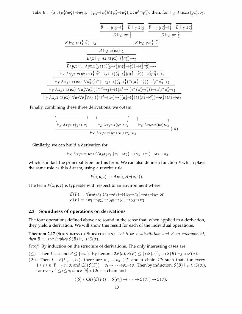
Take B = {x : (ϕ11∩ϕ2

1)→ϕ2,y : (ϕ13→ϕ1

1)∩(ϕ23→ϕ2

1),z : ϕ13∩ϕ2

3}, then, for �E λxyz.x(yz) :σ3:

B �E x : (11∩

21)→2

B �E y : 13→1

1 B �E z : 13

B �E yz : 11

B �E y : 23→2

1 B �E z : 23

B �E yz : 21

B �E yz : 11∩

21

B �E x(yz) : 2

B\z �E λz.x(yz) :(13∩

23)→2

B\y,z �E λyz.x(yz) :((13→1

1)∩(23→2

1))→(13∩

23)→2

�E λxyz.x(yz) :((11∩

21)→2)→((1

3→11)∩(

23→2

1))→(13∩

23)→2

�E λxyz.x(yz) :∀α23.(1

1∩ 21→2)→((1

3→11)∩ (α2

3→21))→1

3∩α23→2

�E λxyz.x(yz) :∀α13∀α2

3.(11∩ 2

1→2)→((α13→1

1)∩ (α23→2

1))→α13∩α2

3→2

�E λxyz.x(yz) :∀α2∀α13∀α3.(1

1∩ 21→α2)→((α1

3→11)∩ (α2

3→21))→α1

3∩α23→α2

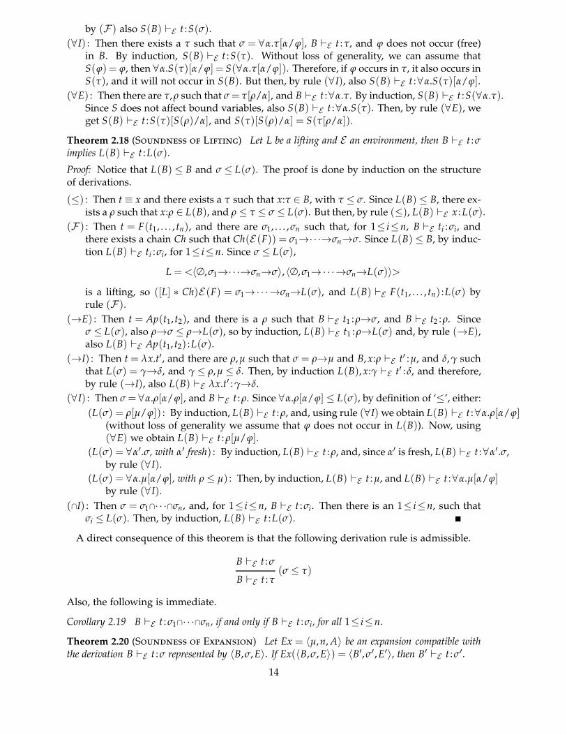
Finally, combining these three derivations, we obtain:

�E λxyz.x(yz) :σ1 �E λxyz.x(yz) :σ2 �E λxyz.x(yz) :σ3(∩I)

�E λxyz.x(yz) :σ1∩σ2∩σ3

Similarly, we can build a derivation for

�E λxyz.x(yz) :∀α3α2α1.(α1→α2)→(α3→α1)→α3→α2

which is in fact the principal type for this term. We can also define a function F which playsthe same role as this λ-term, using a rewrite rule

F(x,y,z)→ Ap(x, Ap(y,z)).

The term F(x,y,z) is typeable with respect to an environment where

E(F) = ∀α3α2α1.(α1→α2)→(α3→α1)→α3→α2 orE(F) = (ϕ1→ϕ2)→(ϕ3→ϕ1)→ϕ3→ϕ2.

2.3 Soundness of operations on derivations

The four operations defined above are sound in the sense that, when applied to a derivation,they yield a derivation. We will show this result for each of the individual operations.

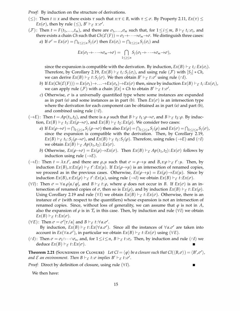
Theorem 2.17 (Soundness of Substitution) Let S be a substitution and E an environment,then B �E t :σ implies S(B) �E t :S(σ).

Proof: By induction on the structure of derivations. The only interesting cases are:

(≤) : Then t ≡ x and B ≤ {x:σ}. By Lemma 2.6(ii), S(B) ≤ {x:S(σ)}, so S(B) �E x :S(σ).(F ) : Then t ≡ F(t1, . . . , tn), there are σ1, . . . ,σn ∈ T and a chain Ch such that, for every

1≤ i≤n, B �E ti :σi and Ch(E(F)) = σ1→·· ·→σn→σ. Then by induction, S(B) �E ti :S(σi),for every 1≤ i≤n; since [S] ∗ Ch is a chain and

([S] ∗ Ch)(E(F)) = S(σ1)→ ·· · → S(σn)→ S(σ),

13

by (F) also S(B) �E t :S(σ).(∀ I) : Then there exists a τ such that σ = ∀α.τ[α/ϕ], B �E t :τ, and ϕ does not occur (free)

in B. By induction, S(B) �E t :S(τ). Without loss of generality, we can assume thatS(ϕ) = ϕ, then ∀α.S(τ)[α/ϕ] = S(∀α.τ[α/ϕ]). Therefore, if ϕ occurs in τ, it also occurs inS(τ), and it will not occur in S(B). But then, by rule (∀ I), also S(B) �E t :∀α.S(τ)[α/ϕ].

(∀E) : Then there are τ,ρ such that σ = τ[ρ/α], and B �E t :∀α.τ. By induction, S(B) �E t :S(∀α.τ).Since S does not affect bound variables, also S(B) �E t :∀α.S(τ). Then, by rule (∀E), weget S(B) �E t :S(τ)[S(ρ)/α], and S(τ)[S(ρ)/α] = S(τ[ρ/α]).

Theorem 2.18 (Soundness of Lifting) Let L be a lifting and E an environment, then B �E t :σimplies L(B) �E t :L(σ).

Proof: Notice that L(B) ≤ B and σ ≤ L(σ). The proof is done by induction on the structureof derivations.

(≤) : Then t ≡ x and there exists a τ such that x:τ ∈ B, with τ ≤ σ. Since L(B) ≤ B, there ex-ists a ρ such that x:ρ ∈ L(B), and ρ ≤ τ ≤ σ ≤ L(σ). But then, by rule (≤), L(B) �E x :L(σ).

(F ) : Then t = F(t1, . . . , tn), and there are σ1, . . . ,σn such that, for 1≤ i≤n, B �E ti :σi, andthere exists a chain Ch such that Ch(E (F)) = σ1→·· ·→σn→σ. Since L(B) ≤ B, by induc-tion L(B) �E ti :σi, for 1≤ i≤n. Since σ ≤ L(σ),

L = <〈∅,σ1→·· ·→σn→σ〉, 〈∅,σ1→·· ·→σn→L(σ)〉>

is a lifting, so ([L] ∗ Ch)E (F) = σ1→·· ·→σn→L(σ), and L(B) �E F(t1, . . . , tn) :L(σ) byrule (F).

(→E) : Then t = Ap(t1, t2), and there is a ρ such that B �E t1 :ρ→σ, and B �E t2 :ρ. Sinceσ ≤ L(σ), also ρ→σ ≤ ρ→L(σ), so by induction, L(B) �E t1 :ρ→L(σ) and, by rule (→E),also L(B) �E Ap(t1, t2) :L(σ).

(→I) : Then t = λx.t′, and there are ρ,µ such that σ = ρ→µ and B, x:ρ �E t′ :µ, and δ,γ suchthat L(σ) = γ→δ, and γ ≤ ρ,µ ≤ δ. Then, by induction L(B), x:γ �E t′ :δ, and therefore,by rule (→I), also L(B) �E λx.t′ :γ→δ.

(∀ I) : Then σ = ∀α.ρ[α/ϕ], and B �E t :ρ. Since ∀α.ρ[α/ϕ] ≤ L(σ), by definition of ‘≤’, either:(L(σ) = ρ[µ/ϕ]) : By induction, L(B) �E t :ρ, and, using rule (∀ I) we obtain L(B) �E t :∀α.ρ[α/ϕ]

(without loss of generality we assume that ϕ does not occur in L(B)). Now, using(∀E) we obtain L(B) �E t : ρ[µ/ϕ].

(L(σ) = ∀α′.σ, with α′ fresh) : By induction, L(B) �E t :ρ, and, since α′ is fresh, L(B) �E t :∀α′.σ,by rule (∀ I).

(L(σ) = ∀α.µ[α/ϕ], with ρ ≤ µ) : Then, by induction, L(B) �E t :µ, and L(B) �E t :∀α.µ[α/ϕ]by rule (∀ I).

(∩I) : Then σ = σ1∩· · ·∩σn, and, for 1≤ i≤n, B �E t :σi. Then there is an 1≤ i≤n, such thatσi ≤ L(σ). Then, by induction, L(B) �E t :L(σ).

A direct consequence of this theorem is that the following derivation rule is admissible.

B �E t :σ(σ ≤ τ)

B �E t :τ

Also, the following is immediate.

Corollary 2.19 B �E t :σ1∩· · ·∩σn, if and only if B �E t :σi, for all 1≤ i≤n.

Theorem 2.20 (Soundness of Expansion) Let Ex = 〈µ,n, A〉 be an expansion compatible withthe derivation B �E t : σ represented by 〈B,σ, E〉. If Ex(〈B,σ, E〉) = 〈B′,σ′, E′〉, then B′ �E t :σ′.

14

Proof: By induction on the structure of derivations.(≤) : Then t ≡ x and there exists τ such that x:τ ∈ B, with τ ≤ σ. By Property 2.11, Ex(τ) ≤

Ex(σ), then by rule (≤), B′ �E x :σ′.(F ) : Then t = F(t1, . . . , tm), and there are σ1, . . . ,σm such that, for 1≤ i≤m, B �E ti :σi, and

there exists a chain Ch such that Ch(E (F)) = σ1→·· ·→σm→σ. We distinguish three cases:a) If σ′ = Ex(σ) =

⋂1≤j≤n Sj(σ) then Ex(σi) =

⋂1≤j≤n Sj(σi) and

Ex(σ1→·· ·→σm→σ) =⋂

1≤j≤n

Sj(σ1→·· ·→σm→σ),

since the expansion is compatible with the derivation. By induction, Ex(B) �E ti :Ex(σi).Therefore, by Corollary 2.19, Ex(B) �E ti :Sj(σi), and using rule (F) with [Sj] ∗ Ch,we can derive Ex(B) �E t :Sj(σ). We then obtain B′ �E t :σ′ using rule (∩I).

b) If Ex(Ch(E(F))) =Ex(σ1)→ . . .→Ex(σn)→Ex(σ) then, since by induction Ex(B) �E ti :Ex(σi),we can apply rule (F) with a chain [Ex] ∗ Ch to obtain B′ �E t :σ′.

c) Otherwise, σ is a universally quantified type where some instances are expandedas in part (a) and some instances as in part (b). Then Ex(σ) is an intersection typewhere the derivation for each component can be obtained as in part (a) and part (b),and combined using rule (∩I).

(→E) : Then t = Ap(t1, t2), and there is a ρ such that B �E t1 :ρ→σ, and B �E t2 :ρ. By induc-tion, Ex(B) �E t1 :Ex(ρ→σ), and Ex(B) �E t2 :Ex(ρ). We consider two cases:

a) If Ex(ρ→σ) =⋂

1≤j≤n Sj(ρ→σ) then also Ex(ρ) =⋂

1≤j≤n Sj(ρ) and Ex(σ) =⋂

1≤j≤n Sj(σ),since the expansion is compatible with the derivation. Then, by Corollary 2.19,Ex(B) �E t1 :Sj(ρ→σ), and Ex(B) �E t2 :Sj(ρ). Therefore, using rules (→E) and (∩I)we obtain Ex(B) �E Ap(t1, t2) :Ex(σ).

b) Otherwise, Ex(ρ→σ) = Ex(ρ)→Ex(σ). Then Ex(B) �E Ap(t1, t2) :Ex(σ) follows byinduction using rule (→E).

(→I) : Then t = λx.t′, and there are ρ,µ such that σ = ρ→µ and B, x:ρ �E t′ :µ. Then, byinduction Ex(B), x:Ex(ρ) �E t′ :Ex(µ). If Ex(ρ→µ) is an intersection of renamed copies,we proceed as in the previous cases. Otherwise, Ex(ρ→µ) = Ex(ρ)→Ex(µ). Since byinduction Ex(B), x:Ex(ρ) �E t′ :Ex(µ), using rule (→I) we obtain Ex(B) �E t :Ex(σ).

(∀ I) : Then σ = ∀α.ρ[α/ϕ], and B �E t : ρ, where ϕ does not occur in B. If Ex(σ) is an in-tersection of renamed copies of σ, then so is Ex(ρ), and by induction Ex(B) �E t :Ex(ρ).Using Corollary 2.19 and rule (∀ I) we obtain Ex(B) �E t :Ex(σ). Otherwise, there is aninstance of σ (with respect to the quantifiers) whose expansion is not an intersection ofrenamed copies. Since, without loss of generality, we can assume that ϕ is not in A,also the expansion of ρ is in Ts in this case. Then, by induction and rule (∀ I) we obtainEx(B) �E t :Ex(σ).

(∀E) : Then σ = σ′[τ/α] and B �E t :∀α.σ′.By induction, Ex(B) �E t :Ex(∀α.σ′). Since all the instances of ∀α.σ′ are taken into

account in Ex(∀α.σ′), in particular we obtain Ex(B) �E t :Ex(σ) using (∀E).(∩I) : Then σ = σ1∩· · ·∩σn, and, for 1≤ i≤n, B �E t : σi. Then, by induction and rule (∩I) we

deduce Ex(B) �E t :Ex(σ).

Theorem 2.21 (Soundness of Closure) Let Cl= 〈ϕ〉 be a closure such that Cl(〈B,σ〉) = 〈B′,σ′〉,and E an environment. Then B �E t :σ implies B′ �E t :σ′.

Proof: Direct by definition of closure, using rule (∀ I).

We then have:

15

Theorem 2.22 (Soundness of Chains) Let B �E t :σ, Ch be a compatible chain, and E an envi-ronment. Then Ch(B �E t :σ) = Ch(B) �E t :Ch(σ).

2.3.1 Type Assignment for Rewrite Rules

Being able to infer a type for a term does not give any guarantee about the typing of the termsin any reduction path out of it. Indeed we need to make sure that the rewrite rules respectthe intended functional behaviour for the function symbols of the signature expressed by theenvironment. The environment, however, does not express a strict condition on the type offunction symbols, leaving room to flexibility by letting us use different consistent instancesof the type of a symbol for different occurrences of it. So, we would like to have a certaindegree of flexibility also in the use of rewriting rules, without losing the property of subjectreduction, which is essential in type systems. In order to achieve this we define a notionof type assignment on rewrite rules, as done in [8], using the notion of principal pair (alsocalled principal typing). The typeability of rules ensures consistency with respect to theenvironment.

Definition 2.23 (Principal pair) 〈P,π〉 is called a principal pair for t with respect to E , ifP �E t :π, and for all B �E t :σ, there is a chain Ch compatible with P �E t :π such thatCh(〈P,π〉) = 〈B,σ〉.

Definition 2.24 i) We say that l → r ∈ R with defined symbol F is typeable with respect to E ,if there are P, and π ∈ T such that:

a) 〈P,π〉 is a principal pair for l with respect to E , and each chain Ch compatible withP �E l :π′ is compatible with P �E r :π.

b) In P �E l :π and P �E r :π all occurrences of F in side conditions to rule (F) aretyped with E (F).

ii) We say that (Σ,R) is typeable with respect to E , if all r ∈ R are.

Notice that, by the formulation of part (i.a), the set of types permitted to occur in the deriva-tion for P �E r : π is restricted.

Note that for a rule F(t1, . . . , tn)→ r to be typeable, E(F) must be of the form σ1→ . . .→σn→σ.Although E(F) cannot have an outermost universal quantifier, its free variables play the samerole as universally quantified variables (since they can be instantiated by substitution oper-ations). In particular, for the polymorphic identity function I we will use E(I) = ϕ→ϕ.

Example 2.25 We show now the type assignment for the rewrite rule D(x)→ Ap(x, x) in anenvironment E where E(D) = (ϕ1→ϕ2)∩ϕ1→ϕ2. Let B = {x:(ϕ1→ϕ2)∩ϕ1}, then

B �E x : ϕ1→ϕ2 B �E x : ϕ1

B �E x : (ϕ1→ϕ2)∩ϕ1

B �E D(x) : ϕ2

Indeed, this is a principal derivation for D(x). In order to type the rewrite rule we have toshow that {x:(ϕ1→ϕ2)∩ϕ1} �E Ap(x, x) : ϕ2, which is easy: let B = {x:(ϕ1→ϕ2)∩ϕ1}, then:

B �E x : (ϕ1→ϕ2) B �E x : ϕ1

B �E Ap(x, x) : ϕ2

16

We will only consider trs+β that are typeable with respect to a given environment E .

2.3.2 Subject Reduction

We will now show that reductions preserve types in our system. In the proof of SubjectReduction we will use one more lemma:

Lemma 2.26 Let E be an environment, t a term, and R a term-substitution.

i) If B �E t :σ and B′ is a basis such that B′ �E xR:ρ for every statement x:ρ ∈ B, then B′ �E tR:σ.ii) If there are B and σ such that B �E tR:σ, then for every x occurring in t there is a type ρx such

that {x:ρx | x occurs in t} �E t :σ, and B �E xR:ρx.

By induction on the structure of derivations.

Theorem 2.27 (Subject Reduction Theorem) If B �E t :σ and t → t′, then B �E t′ :σ.

For a β-reduction step the proof is standard, so we consider only the case of a rewrite step.Let l → r be the typeable rewrite rule applied in the rewrite step t → t′. We will prove thatfor every term-substitution R and type µ, if B �E lR:µ, then B �E rR:µ, which proves thetheorem.Since r is typeable, there are P,π such that 〈P,π〉 is a principal pair for l with respect to E ,and P �E r : π. Suppose R is a term-substitution such that B �E lR:µ. By Lemma 2.26(ii)there is a B′ such that for every x:ρ ∈ B′, B �E xR:ρ, and B′ �E l :µ. Since 〈P,π〉 is aprincipal typing for l with respect to E , by Definition 2.23 there is a chain Ch compatiblewith 〈P,π〉 such that Ch(〈P,π〉) = 〈B′,µ〉. Since P �E r : π, by Theorem 2.22 also B′ �E r :µ.Then by Lemma 2.26(i) B �E rR:µ.

3 Strong Normalisation

As mentioned in the introduction, types serve not only as specifications and as a way toensure that programs ‘cannot go wrong’ during execution, but also to ensure that computa-tions terminate. In fact, this is a well-known property of the intersection system for lc, andof System F, but the situation is different in trs (a rule t →r t may be typeable, although itis obviously non-terminating). In this section, we will focus on the restrictions necessary toobtain a strong normalisation result.

3.1 The General Scheme

Inspired by the work of Jouannaud and Okada [26], who defined a general scheme of recur-sion that ensures termination of higher-order rewrite rules combined with lc, we will definea general scheme for trs+β, such that typeability of (Σ,R) in the (second-order) polymor-phic intersection system defined in this paper implies strong normalisation of all typeableterms.

Definition 3.1 (General Scheme of Recursion) Let Σ be a signature with a set of functionsymbols Fn =Q∪ {F1, . . . , Fn}, where F1, . . . , Fn will be the defined symbols, and Q the setof constructors. We will assume that F1, . . . , Fn are defined incrementally (i.e. there is nomutual recursion), by typeable rules that satisfy the general scheme:

Fi (C[x],y)→ C′ [Fi (C1x,y), . . . , Fi (Cm [x],y),y],

17

where x,y are sequences of variables such that x ⊆ y; C[ ], C′ [ ], C1 , . . . ,Cm [ ] are sequencesof contexts in T(Fi−1,X ); and for every 1≤ j≤m, C[x]>mul Cj [x], where � is the strict sub-term ordering (i.e. > denotes strict super-term) and mul denotes multi-set extension. More-over, in the principal derivation P �E Fi (C[x],y) :π of Fi (C[x],y), the types associated to thevariables y in P are the types of the corresponding arguments of Fi in E(Fi).

This general scheme is a generalisation of primitive recursion. It imposes two main restric-tions on the definition of functions: the terms in the multi-sets Cj [x] are sub-terms of termsin C[x] (this is the ‘primitive recursive’ aspect of the scheme), and the variables x must alsoappear as arguments in the left-hand side of the rule. Both restrictions are essential in theproof of the Strong Normalisation Theorem below. The last one can be replaced by a typingcondition, requiring that the variables in x that are not included in y can only be assignedbase types. Also, instead of the multi-set extension of the subterm ordering, a lexicographicextension can be used, or even a combination of lexicographic and multi-set (see [21] fordetails about these variants of the scheme).

Note that although the general scheme has a primitive recursive aspect, it allows the defi-nition of non-primitive functions thanks to the higher-order features available in trs+β: forexample, Ackermann’s function can be represented.

h(0) → λx.Succ(x)h(Succ(x)) → λy.H(h(x),y)

H(g, 0) → Ap(g,Succ(0))H(g,Succ(y)) → Ap(g, H(g,y))

where Succ is the successor function.Also the rewrite rules of Combinatory Logic are not recursive, so, in particular, satisfy the

scheme.

3.2 The strong normalisation theorem

We shall prove that, when the rewrite rules satisfy the general schema, every typeable term isstrongly normalisable. This will be done using Tait-Girard’s method [22] and the techniquesdevised in [26] in order to cope with some of the difficulties that the presence of algebraicrewriting makes arise.

From now on all the rewrite rules will be assumed to satisfy the general schema.In the following, a sequence e1, . . . , en of elements will be denoted by e. The length of the

sequence will be denoted by |e| (so |e1, . . . , en| = n). In this section we shall not distinguishbetween free and bound type variables. Type variables will be denoted by ϕ, ϕ′, ϕ1, . . .. Recallthat a term is called neutral if it is not an abstraction.

Definition 3.2 A Reducibility Candidate of type τ is a set Rτ of terms typeable with τ andsuch that:(C1) : If t ∈ Rτ , then t is strongly normalisable, SN (t).(C2) : If t ∈ Rτ and t →∗ t′, then t′ ∈ Rτ .(C3) : If t is neutral and typeable with type τ, and if, for every u, t → u implies u ∈ Rτ , then

t ∈ Rτ .

Note that any reducibility candidate contains all the term-variables and that, for any typeρ, SN ρ is a reducibility candidate.

18

Definition 3.3 Let ρ be a type, and let Rγ be a sequence of reducibility candidates Rγ11 , . . . ,Rγn

nsuch that |Rγ|= |ϕ|, where {ϕ} ⊇ FV(ρ); then we can define the set of terms Red ρ[Rγ/ϕ] byinduction on ρ, as follows:

(ρ ≡ s) : Red s[Rγ/ϕ] = SN s.(ρ ≡ ϕi) : Red ϕi [Rγ/ϕ] =Rγi

i .

(ρ ≡ σ∩τ) : Red σ∩τ[Rγ/ϕ] = Red σ[Rγ/ϕ]∩Red τ[Rγ/ϕ].(ρ ≡ σ→τ) : Red σ→τ[Rγ/ϕ] is the set of terms t typeable with (σ→τ)[γ/ϕ] and such that,

for every u ∈ Red σ[Rγ/ϕ], Ap(t,u) ∈ Red τ[Rγ/ϕ].(ρ ≡ ∀α′.τ) : Red∀α′.τ[Rγ/ϕ] is the set of terms t typeable with ∀α′.τ[γ/ϕ] and such that, for

any type δ and reducibility candidate Sδ, t ∈ Red τ [Rγ/ϕ,Sδ/α′].

From now on, when considering a sequence Rγ in a Red ρ[Rγ/ϕ], we shall always tacitlyassume |Rγ|= |ϕ| and {ϕ} ⊇ FV(ρ).

Lemma 3.4 Red ρ[Rγ/ϕ] is a reducibility candidate of type ρ[γ/ϕ].

Proof: By induction on the structure of ρ.

(ρ ≡ s) : By definition Red ρ[Rγ/ϕ] = SN s. It is straightforward to check that SN s satisfies(C1), (C2) and (C3).

(ρ ≡ ϕi) : Immediate by definition, since Rγii is a reducibility candidate of type γi.

(ρ ≡ σ∩τ) : We have first to show that, if t ∈ Red σ[Rγ/ϕ]∩Red τ[Rγ/ϕ], then t is typeablewith (σ∩τ)[γ/ϕ]. By induction Red σ[Rγ/ϕ] and Red τ[Rγ/ϕ] are reducibility candidatesof type σ[γ/ϕ] and τ[γ/ϕ], respectively. Hence t is typeable by σ[γ/ϕ] and τ[γ/ϕ]. Since(σ∩τ)[γ/ϕ]≡ σ[γ/ϕ]∩τ[γ/ϕ], by definition of our system we get that t is typeable with(σ∩τ)[γ/ϕ]. We have now to prove the other properties of a reducibility candidate,namely (C1), (C2) and (C3). These are easily inferred by the fact that Red ρ[Rγ/ϕ] is theintersection of two reducibility candidates.

(ρ ≡ σ→τ) : By definition 3.3 we have that if t ∈ Red ρ[Rγ/ϕ] then t is typeable with (σ→τ)[γ/ϕ].We can prove now the other properties which must hold for a reducibility candidate.(C1) : Let t ∈ Red ρ[Rγ/ϕ]. By induction both Red σ[Rγ/ϕ] and Red τ[Rγ/ϕ] are re-

ducibility candidates. Hence, since any reducibility candidate contains all the vari-ables, by Definition 3.3, we have that Ap(t, x) ∈ Red τ[Rγ/ϕ] and, by (C1), Ap(t, x)is strongly normalisable. Thus also t is strongly normalisable.

(C2) : Let t ∈ Red ρ[Rγ/ϕ], with t →∗ t′, and let u ∈ Red σ[Rγ/ϕ]. By Definition 3.3, wehave Ap(t,u) ∈ Red τ [Rγ/ϕ]. Hence Ap(t,u)→∗ Ap(t′,u) and Ap(t′,u) ∈ Red τ[Rγ/ϕ],by (C2). By Subject Reduction (Theorem 2.27) and (C2), we obtain t′ ∈ Red ρ[Rγ/ϕ].

(C3) : Let t be neutral and typeable with ρ[γ/ϕ], and let us assume that

∀u.t → u ⇒ u ∈ Red ρ[Rγ/ϕ].

We have to prove that

∀w.(w ∈ Red σ[Rγ/ϕ] ⇒ Ap(t,w) ∈ Red τ[Rγ/ϕ]).

Let then v ∈ Red σ[Rγ/ϕ]. Since t is typeable with (σ→τ)[γ/ϕ] and, by induction,v is typeable with σ[γ/ϕ], Ap(t,v) is typeable with τ[γ/ϕ]. Moreover Ap(t,v) isa neutral term and thus, since (C3) holds for Red τ[Rγ/ϕ] by induction, to provethat Ap(t,v) ∈ Red τ [Rγ/ϕ], it suffices to show that for any t such that Ap(t,v) →t, t ∈ Red τ[Rγ/ϕ]. By (C1) for Red σ[Rγ/ϕ], v is strongly normalisable. We nowproceed by induction on the height of the reduction tree of v.

Since t is neutral, the reduction from Ap(t,v) to t has necessarily to occur eitherin t or in v.

19

1) If t ≡ Ap(t′,v) with t → t′ then, by our assumption t′ ∈ Red ρ[Rγ/ϕ] and hence,by definition of Red ρ[Rγ/ϕ] we have Ap(t′,v) ∈ Red τ [Rγ/ϕ].

2) If t ≡ Ap(t,v′) with v→ v′ , then, by (C2) for Red σ[Rγ/ϕ] we have v′ ∈ Red σ[Rγ/ϕ].Since the reduction tree of v′ is strictly shorter than the one of v, by induction weobtain Ap(t,v′) ∈ Red τ [Rγ/ϕ].

(ρ ≡ ∀ϕ′.τ) : Any element of Red∀ ϕ′.τ[Rγ/ϕ] is typeable with ∀ϕ′.τ[γ/ϕ] by definition. Wenow check that the other conditions hold.(C1) : Let t ∈ Red∀ ϕ′.τ[Rγ/ϕ], let δ be an arbitrary type and let Sδ be a reducibility can-

didate for δ (the strongly normalisable terms typeable with δ, for instance). Then,by definition, t ∈ Red τ[Rγ/ϕ,Sδ/ϕ′]. Since for Red τ[Rγ/ϕ,Sδ/ϕ′] the induction hy-pothesis applies, by (C1) we get that t is strongly normalisable.

(C2) : Let t ∈ Red∀ ϕ′ .τ[Rγ/ϕ] with t →∗ t′. By definition, for all types δ and candidatesSδ we have t ∈ Red τ[Rγ/ϕ,Sδ/ϕ′]. Hence, by induction and (C2), t′ ∈ Red τ [Rγ/ϕ,Sδ/ϕ′]for all types δ and candidates Sδ. Thus, by definition and Subject Reduction,t′ ∈ Red∀ ϕ′.τ[Rγ/ϕ].

(C3) : Let t be neutral and typeable with ∀ϕ′.τ[γ/ϕ] and let us assume

∀u.t → u ⇒ u ∈ Red∀ ϕ′.τ[Rγ/ϕ].

Taking any type δ and any candidate Sδ for it, we have, by definition, that

∀u.t → u ⇒ u ∈ Red τ[Rγ/ϕ,Sδ/ϕ′].

Since the induction hypothesis applies for Red τ[Rγ/ϕ,Sδ/ϕ′], by (C3) we havethat, for any type δ and any candidate Sδ for it, t ∈ Red τ[Rγ/ϕ,Sδ/ϕ′], and hence,by definition, t ∈ Red∀ ϕ′.τ[Rγ/ϕ].

Lemma 3.5 (Red-substitution Lemma)

Red σ[τ/ϕ] [Rγ/ϕ] ≡ Red σ[Rγ/ϕ,Red τ/ϕ[Rγ/ϕ]].

Proof: By induction on the structure of σ.

Lemma 3.6 Let τ ≤ σ. Then, for any reducibility candidates Rγ:

Red τ[Rγ/ϕ] ⊆ Red σ[Rγ/ϕ].

Proof: By induction on the definition of ≤ .(∀1≤ i≤n (n ≥ 1) [σ1∩· · ·∩σn ≤ σi]) : Easy.(∀1≤ i≤n (n ≥ 1)σ ≤ σi ⇒ σ ≤ σ1∩· · ·∩σn) : Easy.(σ ≤ σ′ & τ ≤ τ′ ⇒ σ′→τ ≤ σ→τ′) : Let t ∈ Red σ′→τ[Rγ/ϕ]. Then, by definition, t is ty-

peable with σ′→τ and

∀u.(u ∈ Red σ′[Rγ/ϕ] ⇒ Ap(t,u) ∈ Red τ[Rγ/ϕ]).

In order to prove that t ∈ Red σ→τ′[Rγ/ϕ] we first notice that, by Theorem 2.18, t is also

typeable with σ→τ′. Now, to show that

∀u.(u ∈ Red σ[Rγ/ϕ] ⇒ Ap(t,u) ∈ Red τ′[Rγ/ϕ]),

take u ∈ Red σ[Rγ/ϕ]. By induction Red σ[Rγ/ϕ]⊆ Red σ′[Rγ/ϕ]. Hence u ∈ Red σ′

[Rγ/ϕ]and by assumption Ap(t,u) ∈ Red τ [Rγ/ϕ]. Again by induction, Ap(t,u) ∈ Red τ′

[Rγ/ϕ].

20

(∀ϕ′.σ ≤ σ[τ/ϕ′ ]) : Let t ∈ Red∀ ϕ′.σ[Rγ/ϕ]. By definition, for any type δ and reducibilitycandidate Sδ, t ∈ Red σ[Rγ/ϕ,Sδ/ϕ′]. In particular, t ∈ Red σ[Rγ/ϕ,Red τ[Rγ/ϕ]/ϕ′]. Bythe Red-substitution Lemma 3.5, we obtain t ∈ Red σ[τ/ϕ′ ][Rγ/ϕ].

(σ ≤ τ ⇒ ∀ϕ′.σ ≤ ∀ϕ′τ) : By induction, for any reducibility candidates Rγ, Sδ:

Red τ[Rγ/ϕ,Sδ/ϕ′] ⊆ Red σ[Rγ/ϕ,Sδ/ϕ′].

Then, by Definition 3.3, it follows that for any reducibility candidate Rγ

Red∀ ϕ′.τ[Rγ/ϕ] ⊆ Red∀ ϕ′.σ[Rγ/ϕ].

(σ ≤ ∀ϕ′.σ with ϕ′ �∈ FV(σ)) : Since ϕ′ �∈ FV(σ), for any type δ and candidate Sδ, Red σ[Rγ/ϕ]≡Red σ[Rγ/ϕ,Sδ/ϕ′]. Hence, by definition, we have that Red σ[Rγ/ϕ] ⊆ Red∀ ϕ.σ[Rγ/ϕ].

Definition 3.7 i) A term t typeable with type τ is reducible if it is in Red τ[SN X/X], whereX are the free variables of τ.

ii) Let B = {x1:σ1, . . . , xn:σn} be a basis and let FV(σ1, . . . ,σn) ⊆ {ϕ}. Moreover, let γ be asequence of types such that |γ|= |ϕ| and let Rγ be a sequence of reducibility candidates.A term-substitution R is Rγ-reducible for B if, for every xi:σi ∈ B, xiR ∈ Red σi [Rγ/ϕ].

Terms can, as usual, be seen as trees; the sub-term of t at position p will be denoted by t|p,and t[u]p will denote the result of replacing, in t, the sub-term at position p by u.

We shall prove our strong normalisation result by showing that every typeable term isreducible. This implies strong normalisation by Lemma 3.4 and (C1). In order to show thatany typeable term is reducible we need to prove a stronger property, for which we will needthe following ordering.

Definition 3.8 i) Let ‘>IN’ denote the standard ordering on natural numbers, and lex, muldenote respectively the lexicographic and multi-set extension of an ordering. Let ‘>· ’ standfor the well-founded encompassment ordering, i.e. u>· v if u �≡ v modulo renaming ofvariables, and u|p = vR for some position p ∈ u and term-substitution R. Note that en-compassment contains strict super-term (‘>’).

ii) We define the ordering ‘�SN’ on triples – consisting of a natural number, a term, and amulti-set of terms – as the object

(>IN, >· , (→∪>)mul)lex.

iii) We will interpret the term uR by the triple 〈i,u,{R}〉 = I(uR), where

– i is the maximal super-index of the function symbols belonging to u,– {R} is the multi-set {xR | x ∈ Var(u)}.

These triples are compared in the ordering ‘�SN’.

When R is Rγ-reducible for some basis containing the free variables of u, then, by (C1),every t in {R} is strongly normalisable, so the rewrite relation ‘→’ is well-founded on {R}.Also, since the union of the relation ‘>’ with a terminating rewrite relation is well-founded[18], the relation ‘(→∪>)mul’ is well-founded on {R}. Hence, with such term-substitutions,‘�SN’ is a well-founded ordering.

We will use ‘�SNn ’ when we want to indicate that the n-th element of the triple has de-

creased and the first n−1 have not increased.We would like to stress that we do not just interpret terms, but pairs of terms and term-

substitutions. This implies that although it can be that the terms tR1 and tR2 are equal, theirinterpretations need not be equal as well.

We now come to the main theorem of this section.

21

Property 3.9 Let B �E t :σ, where B = {x1:σ1, . . . , xn:σn}, and let FV(σ1, . . . ,σn,σ) ⊆ {ϕ}. Then,given a sequence of types γ such that |γ| = |ϕ| and a sequence of reducibility candidates Rγ, if R isa term-substitution that is Rγ-reducible for B, then tR ∈ Red σ[Rγ/ϕ].

Proof: See the Appendix.

Theorem 3.10 (Strong Normalisation) Any typeable term is strongly normalisable.

Proof: By Property 3.9, it easily follows that any typeable term is reducible. Strong normali-sation then follows from Lemma 3.4 and (C1).

4 Confluence

Using the previous strong normalisation result, we are going to show that the absence ofcritical pairs in a typeable trs+β implies confluence on typeable terms.

Definition 4.1 If l → r and s → t are two rewrite rules (we assume that the variables wererenamed so that there is no variable that occurs in both), p is the position of a non-variablesubterm of s and µ is a most general unifier of s|p and l, then (tµ, sµ[rµ]p) is a critical pairformed from those rules. Note that the second rule may be a renamed version of the first. Inthis case a super-position at the root position is not considered a critical pair.

We will prove that the absence of critical pairs implies local confluence, and use Newman’sLemma [33] to deduce confluence from strong normalisation and local confluence. Let usrecall the definition of local confluence:

Definition 4.2 A reduction relation → is locally confluent on a set T of terms, if for anyt,v1,v2 ∈ T such that t → v1 and t → v2, there exists v3 ∈ T such that v1 →∗ v3 and v2 →∗ v3.

Theorem 4.3 A typeable trs+β (Σ,R) is locally confluent on typeable terms if it does not havecritical pairs.

By the Subject Reduction Theorem, all rewrite sequences starting from a typeable termremain inside the set of typeable terms. We study the interactions between the two classesof reductions we have: β-reductions, and reductions using R.The absence of critical pairs guarantees no super-position between the rewrite rules. It iswell-known that this implies local confluence of first-order rules on algebraic terms. Theextension to terms containing λ-abstractions is standard: we abstract with term-variablesthe sub-terms that have a λ at the root, taking care of using the same variable for identicalsub-terms since rewrite rules may be non left-linear (see [9] for details). The extension torules containing λ-abstraction only in the right-hand side (as in our systems) is alsostraightforward.Since β-reductions are confluent on λ-terms containing constants, the only remaining caseto study is the interaction of β-reductions with reductions using R. But since by definitionof rewrite rule, the symbol Ap cannot appear in a left-hand side, there is no super-positionbetween β and other rules. This completes the proof.

5 Restriction to Rank2

In this section, we will present a decidable restriction of the type system as presented above,based on types of rank 2. Although the Rank 2 intersection system and the Rank 2 poly-morphic system for lc type exactly the same set of terms [37], their combination results ina system with more expressive power: polymorphism can be expressed directly (using the

22

universal quantifier) and, more importantly, as we will show below, every typeable term hasa principal type; the latter property does not hold in a system without intersection.

5.1 Rank 2 type assignment

In this subsection, we will briefly discuss a notion of Rank 2 type assignment (the systempresented here is not the only one possible: a variant could be to consider also the emptyintersection, i.e. to use the type constant ω, but we will not take that direction here).

The polymorphic intersection types of Rank 2, T2, are a true subset of the set of polymor-phic intersection types as presented in Definition 2.1.

Definition 5.1 (Rank 2 types and bases) i) We define polymorphic intersection types ofRank 2 in layers:

TC ::= ϕ | s | (TC → TC) (Curry types)T ∀

C ::= TC | (∀α.T ∀C[α/ϕ]) (Quantified Curry types)

T1 ::= (T ∀C∩ · · · ∩T ∀

C) (Rank 1 types)T2 ::= ϕ | (T1 → T2) (Rank 2 types)

We omit brackets as before.ii) A Rank 2 basis is a basis in which all types are in T1.

Below, we will define a unification procedure that will recursively go through types. How-ever, using the sets defined above, not every sub-type of a type in T2 is a type in that same set.For example, α→ϕ is not a type in any of the sets defined above; however, ∀α.α→ϕ ∈ T ∀

C,and therefore it can be that, when going through types in T2 recursively, α→ϕ has to be dealtwith. Since the distinction between free and bound variables is essential, we introduce, forevery set Ti defined above, also the set T ′

i of types, that contains also free occurrences of αs.We will not always use the ‘′’ when speaking of these sets, however; it will be clear from thecontext which set is intended.

As for T , we will consider a relation on types, ≤2, but one that is not the restriction to T2of the relation ≤ defined in Definition 2.2; notice that the part corresponding to ‘σ ≤2 ∀α.σ,if α not in σ’ is missing.

Definition 5.2 (Relations on types) On types, the pre-order (i.e. reflexive and transitiverelation) ≤2 is generated by the following rules:

σ1∩· · ·∩σn ≤2 σi, (1≤ i≤n)∀α.σ[α/ϕ] ≤2 σ[τ/ϕ], (τ ∈ TC)

∀1≤ i≤n.σ ≤2 σi ⇒ σ ≤2 σ1∩· · ·∩σn (n ≥ 1)ρ ≤2 σ,τ ≤2 µ ⇒ σ→τ ≤2 ρ→µ, (ρ,σ ∈ T1, τ,µ ∈ T2)

σ ≤2 τ ⇒ ∀α.σ[α/ϕ] ≤2 ∀α.τ[α/ϕ].

The equivalence relation ‘∼2’ is defined by: σ ∼2 τ ⇐⇒ σ ≤2 τ ≤2 σ, and we extend ‘≤2’ tobases in the same way as done for ‘≤’.

For ≤2, the following properties hold:

Lemma 5.3 i) If σ ∈ T1, σ ≤2 τ ∈ T2, and σ does not contain ‘∀’, then neither does τ.ii) If σ ≤2 τ1∩· · ·∩τn, then, for all 1≤ i≤n, σ ≤2 τi.

Proof: Easy.

23

The Rank 2 versions for the various operations as presented below are defined in muchthe same way as in [6], with the exception of the operation of closure and lifting, that werenot used there.

The first three operations used for the Rank 2 system are straightforward variants of oper-ations defined for the full system.

Definition 5.4 i) Substitution (ϕ �→ ρ) : T2 → T2 is defined as in Definition 2.5, but with therestriction that ρ ∈ TC. For the sake of clarity, and in order to avoid writing [S1, . . . ,Sn]for a chain of single type-variable substitutions, we will close the set of substitution forcomposition ‘◦’: for substitutions S1,S2, the substitution S2◦S1 is defined as S2◦S1(σ) =S2(S1(σ)). We use IdS for the substitution that replaces all variables by themselves, andwrite S for the set of all substitutions.

ii) Lifting is defined as in Definition 2.12, but with the restriction that ‘≤’ is taken to be ‘≤2’of Definition 5.2.

iii) Closure is defined as in Definition 2.13 as a pair of types 〈σ, ϕ〉, with the restriction thatσ ∈ T ∀

C:〈σ, ϕ〉(〈B,τ1∩· · ·∩τn〉) = 〈B,τ′

1∩· · ·∩τ′n〉

where, for all 1≤ i≤n,

τ′i = ∀α.σ[α/ϕ], if τi = σ, and ϕ does not appear in B (α is a fresh variable), and

τ′i = τi, otherwise.

The variant of expansion used in the Rank 2 system is quite different from that of Defini-tion 2.9. The reason for this is that expansion, normally, increases the rank of a type:

〈ϕ1,2〉(〈{x:ϕ1→ϕ2}, ϕ1〉)(ϕ1→ϕ2) = (ϕ11∩ϕ2

1)→ϕ2,

a feature that is of course not sound when present within a system that limits the rank oftypes. Since below expansion is only used in very precise situations (within the procedureunify∀ 2, and in the proof of Theorem 5.29), the solution is relatively easy: in the context ofRank 2 types, expansion is only called on types in T ∀

C, so it is defined to work well there,by replacing all types by an intersection; in particular, intersections are not created at the leftof an arrow.

Definition 5.5 Let B be a Rank 2 basis, σ ∈ T2, and n ≥ 1. The n-fold Rank 2 expansion withrespect to the pair 〈B,σ〉, n〈B,σ〉 : T2 →T2 is constructed as follows: Suppose V = {ϕ1, . . . , ϕm}is the set of all (free) variables occurring in 〈B,σ〉. Choose m× n different variables ϕ1

1, . . . , ϕn1 ,

. . . , ϕ1m, . . . , ϕn

m, such that each ϕij (1≤ i≤n, 1≤ j≤m) does not occur in V. Let Si be the

substitution that replaces every ϕj by ϕij. Then Rank 2 expansion is defined on types, bases,

and pairs, respectively, by:

n〈B,σ〉(τ) = S1(τ)∩ · · · ∩Sn(τ),n〈B,σ〉(B′) = {x:n〈B,σ〉(ρ) | x:ρ ∈ B},n〈B,σ〉(〈B′,σ′〉) = 〈n〈B,σ〉(B′),n〈B,σ〉(σ

′)〉.

Notice that, if τ ∈ T2, it can be that S1(τ)∩ · · · ∩Sn(τ) is not a legal type. However, sinceeach Si(τ) ∈ T2, for 1≤ i≤n, for the sake of clarity, we will not treat it separately (see alsoLemma 5.13).

Notice that we have no need for the third parameter ‘A’ in this notion of expansion. SinceRank 2 expansion essentially is just the combination of a number of substitutions by means ofrule (∩I), we do not need to calculate the set of affected types, for which the third parameterwas added.

24

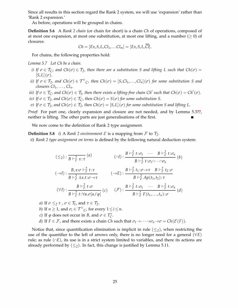
Since all results in this section regard the Rank 2 system, we will use ‘expansion’ rather than‘Rank 2 expansion.’

As before, operations will be grouped in chains.

Definition 5.6 A Rank 2 chain (or chain for short) is a chain Ch of operations, composed ofat most one expansion, at most one substitution, at most one lifting, and a number (≥ 0) ofclosures:

Ch = [Ex,S,L,Cl1, . . .Clm] = [Ex,S,L,Cl].

For chains, the following properties hold:

Lemma 5.7 Let Ch be a chain.i) If σ ∈ TC, and Ch(σ) ∈ T2, then there are a substitution S and lifting L such that Ch(σ) =[S,L] (σ).

ii) If σ ∈ T2, and Ch(σ) ∈ T ∀C, then Ch(σ) = [S,Cl1, . . . ,Cln] (σ) for some substitution S and

closures Cl1, . . . , Cln.iii) If σ ∈ TC, and Ch(σ) ∈ T1, then there exists a lifting-free chain Ch′ such that Ch(σ) = Ch′(σ).iv) If σ ∈ T2, and Ch(σ) ∈ TC, then Ch(σ) = S(σ) for some substitution S.v) If σ ∈ T2, and Ch(σ) ∈ T2, then Ch(σ) = [S,L] (σ) for some substitution S and lifting L.

Proof: For part one, clearly expansion and closure are not needed, and by Lemma 5.3??,neither is lifting. The other parts are just generalisations of the first.

We now come to the definition of Rank 2 type assignment.

Definition 5.8 i) A Rank 2 environment E is a mapping from F to T2.ii) Rank 2 type assignment on terms is defined by the following natural deduction system:

(≤2) : (a)B �2

E x :τ (∩I) :B �2

E t : σ1 · · · B �2E t :σn

(b)B �2

E t : σ1∩· · ·∩σn

(→I) :B, x:σ �2

E t :τ

B �2E λx.t :σ→τ

(→E) :B �2

E t1 :σ→τ B �2E t2 :σ

B �2E Ap(t1, t2) :τ

(∀ I) :B �2

E t :σ(c)

B �2E t :∀α.σ[α/ϕ]

(F) :B �2

E t : σ1 · · · B �2E t :σn

(d)B �2

E F(t1, . . . , tn) :σ

a) If σ ≤2 τ , σ ∈ T1, and τ ∈ T2.b) If n ≥ 1, and σi ∈ T ∀

C, for every 1≤ i≤n.c) If ϕ does not occur in B, and σ ∈ T∀

C .d) If F ∈ F , and there exists a chain Ch such that σ1→·· ·→σn→σ = Ch(E (F)).

Notice that, since quantification elimination is implicit in rule (≤2), when restricting theuse of the quantifier to the left of arrows only, there is no longer need for a general (∀E)rule; as rule (∩E), its use is in a strict system limited to variables, and there its actions arealready performed by (≤2). In fact, this change is justified by Lemma 5.11.

25

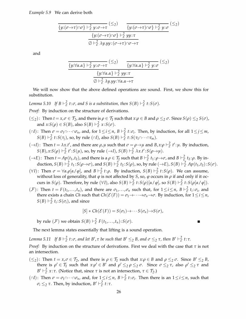
Example 5.9 We can derive both

(≤2){y:(σ→τ)∩σ} �2E y :σ→τ

(≤2){y:(σ→τ)∩σ} �2E y :σ

{y:(σ→τ)∩σ} �2E yy :τ

∅ �2E λy.yy :(σ→τ)∩σ→τ

and

(≤2){y:∀α.α} �2E y :σ→τ

(≤2){y:∀α.α} �2E y :σ

{y:∀α.α} �2E yy :τ

∅ �2E λy.yy :∀α.α→τ

We will now show that the above defined operations are sound. First, we show this forsubstitution.

Lemma 5.10 If B �2E t :σ, and S is a substitution, then S(B) �2

E t :S(σ).

Proof: By induction on the structure of derivations.

(≤2) : Then t= x,σ ∈ T2, and there is ρ ∈ T1 such that x:ρ ∈ B and ρ ≤2 σ. Since S(ρ) ≤2 S(σ),and x:S(ρ) ∈ S(B), also S(B) �2

E x :S(σ).

(∩I) : Then σ = σ1∩· · ·∩σn, and, for 1≤ i≤n, B �2E t :σi. Then, by induction, for all 1≤ j≤m,

S(B) �2E t :S(τj), so, by rule (∩I), also S(B) �2

E t :S(τ1∩· · ·∩τm).

(→I) : Then t = λx.t′, and there are ρ,µ such that σ = ρ→µ and B, x:ρ �2E t′ :µ. By induction,

S(B), x:S(ρ) �2E t′ :S(µ), so, by rule (→I), S(B) �2

E λx.t′ :S(ρ→µ).

(→E) : Then t =Ap(t1, t2), and there is a ρ ∈ T1 such that B �2E t1 :ρ→σ, and B �2

E t2 :ρ. By in-duction, S(B) �2

E t1 :S(ρ→σ), and S(B) �2E t2 :S(ρ), so, by rule (→E), S(B) �2

E Ap(t1, t2) :S(σ).

(∀ I) : Then σ = ∀α.ρ[α/ϕ], and B �2E t :ρ. By induction, S(B) �2

E t :S(ρ). We can assume,without loss of generality, that ϕ is not affected by S, so, ϕ occurs in ρ if and only if it oc-curs in S(ρ). Therefore, by rule (∀ I), also S(B) �2

E t :S(ρ)[α/ϕ], so S(B) �2E t :S(ρ[α/ϕ]).

(F ) : Then t = F(t1, . . . , tn), and there are σ1, . . . ,σn such that, for 1≤ i≤n, B �2E ti :σi, and

there exists a chain Ch such that Ch(E (F)) = σ1→·· ·→σn→σ. By induction, for 1≤ i≤n,S(B) �2

E ti :S(σi), and since

[S] ∗ Ch(E (F)) = S(σ1)→·· ·S(σn)→S(σ),

by rule (F) we obtain S(B) �2E F(t1, . . . , tn) :S(σ).

The next lemma states essentially that lifting is a sound operation.

Lemma 5.11 If B �2E t :σ, and let B′,τ be such that B′ ≤2 B, and σ ≤2 τ, then B′ �2

E t :τ.

Proof: By induction on the structure of derivations. First we deal with the case that τ is notan intersection.

(≤2) : Then t = x,σ ∈ T2, and there is ρ ∈ T1 such that x:ρ ∈ B and ρ ≤2 σ. Since B′ ≤2 B,there is ρ′ ∈ T1 such that x:ρ′ ∈ B′ and ρ′ ≤2 ρ ≤2 σ. Since σ ≤2 τ, also ρ′ ≤2 τ andB′ �2

E x :τ. (Notice that, since τ is not an intersection, τ ∈ T2.)

(∩I) : Then σ = σ1∩· · ·∩σn, and, for 1≤ i≤n, B �2E t :σi. Then there is an 1≤ i≤n, such that

σi ≤2 τ. Then, by induction, B′ �2E t :τ.

26

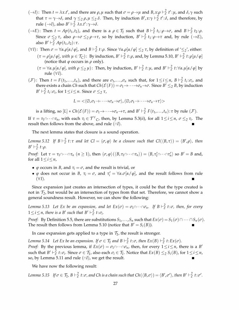
(→I) : Then t = λx.t′, and there are ρ,µ such that σ = ρ→µ and B, x:ρ �2E t′ :µ, and δ,γ such

that τ = γ→δ, and γ ≤2 ρ,µ ≤2 δ. Then, by induction B′, x:γ �2E t′ :δ, and therefore, by

rule (→I), also B′ �2E λx.t′ :γ→δ.

(→E) : Then t = Ap(t1, t2), and there is a ρ ∈ T1 such that B �2E t1 :ρ→σ, and B �2

E t2 :ρ.Since σ ≤2 τ, also ρ→σ ≤2 ρ→τ, so by induction, B′ �2

E t1 :ρ→τ and, by rule (→E),also B′ �2

E Ap(t1, t2) :τ.

(∀ I) : Then σ = ∀α.ρ[α/ϕ], and B �2E t :ρ. Since ∀α.ρ[α/ϕ] ≤2 τ, by definition of ‘≤2’, either:

(τ = ρ[µ/ϕ], with µ ∈ TC) : By induction, B′ �2E t :ρ, and, by Lemma 5.10, B′ �2

E t :ρ[µ/ϕ](notice that ϕ occurs in ρ only).

(τ = ∀α.µ[α/ϕ], with ρ ≤2 µ) : Then, by induction, B′ �2E t :µ, and B′ �2

E t :∀α.µ[α/ϕ] byrule (∀ I).

(F ) : Then t = F(t1, . . . , tn), and there are σ1, . . . ,σn such that, for 1≤ i≤n, B �2E ti :σi, and

there exists a chain Ch such that Ch(E (F)) = σ1→·· ·→σn→σ. Since B′ ≤2 B, by inductionB′ �2

E ti :σi, for 1≤ i≤n. Since σ ≤2 τ,

L = <〈∅,σ1→·· ·→σn→σ〉, 〈∅,σ1→·· ·→σn→τ〉>

is a lifting, so [L] ∗ Ch(E (F)) = σ1→·· ·→σn→τ, and B′ �2E F(t1, . . . , tn) :τ by rule (F).

If τ = τ1∩· · ·∩τn, with each τi ∈ T ∀C, then, by Lemma 5.3(ii), for all 1≤ i≤n, σ ≤2 τi. The

result then follows from the above, and rule (∩I).

The next lemma states that closure is a sound operation.

Lemma 5.12 If B �2E t :τ and let Cl = 〈σ, ϕ〉 be a closure such that Cl(〈B,τ〉) = 〈B′,ρ〉, then

B′ �2E t :ρ.

Proof: Let τ = τ1∩· · ·∩τn (n ≥ 1), then 〈σ, ϕ〉(〈B,τ1∩· · ·∩τn〉) = 〈B,τ′1∩· · ·∩τ′

n〉 so B′ = B and,for all 1≤ i≤n,

• ϕ occurs in B, and τi = σ, and the result is trivial, or• ϕ does not occur in B, τi = σ, and τ′

i = ∀α.σ[α/ϕ], and the result follows from rule(∀ I).

Since expansion just creates an intersection of types, it could be that the type created isnot in T2, but would be an intersection of types from that set. Therefore, we cannot show ageneral soundness result. However, we can show the following:

Lemma 5.13 Let Ex be an expansion, and let Ex(σ) = σ1∩· · ·∩σn. If B �2E t :σ, then, for every

1≤ i≤n, there is a B′ such that B′ �2E t :σi.

Proof: By Definition 5.5, there are substitutions S1, . . . ,Sn such that Ex(σ) = S1(σ)∩ · · · ∩Sn(σ).The result then follows from Lemma 5.10 (notice that B′ = Si(B)).

In case expansion gets applied to a type in T1, the result is stronger.

Lemma 5.14 Let Ex be an expansion. If σ ∈ T1 and B �2E t :σ, then Ex(B) �2

E t :Ex(σ).Proof: By the previous lemma, if Ex(σ) = σ1∩· · ·∩σn, then, for every 1≤ i≤n, there is a B′

such that B′ �2E t :σi. Since σ ∈ T1, also each σi ∈ T1. Notice that Ex(B) ≤2 Si(B), for 1≤ i≤n,

so, by Lemma 5.11 and rule (∩I), we get the result.

We have now the following result:

Lemma 5.15 If σ ∈ T1, B �2E t :σ, and Ch is a chain such that Ch(〈B,σ〉) = 〈B′,σ′〉, then B′ �2

E t :σ′.

27

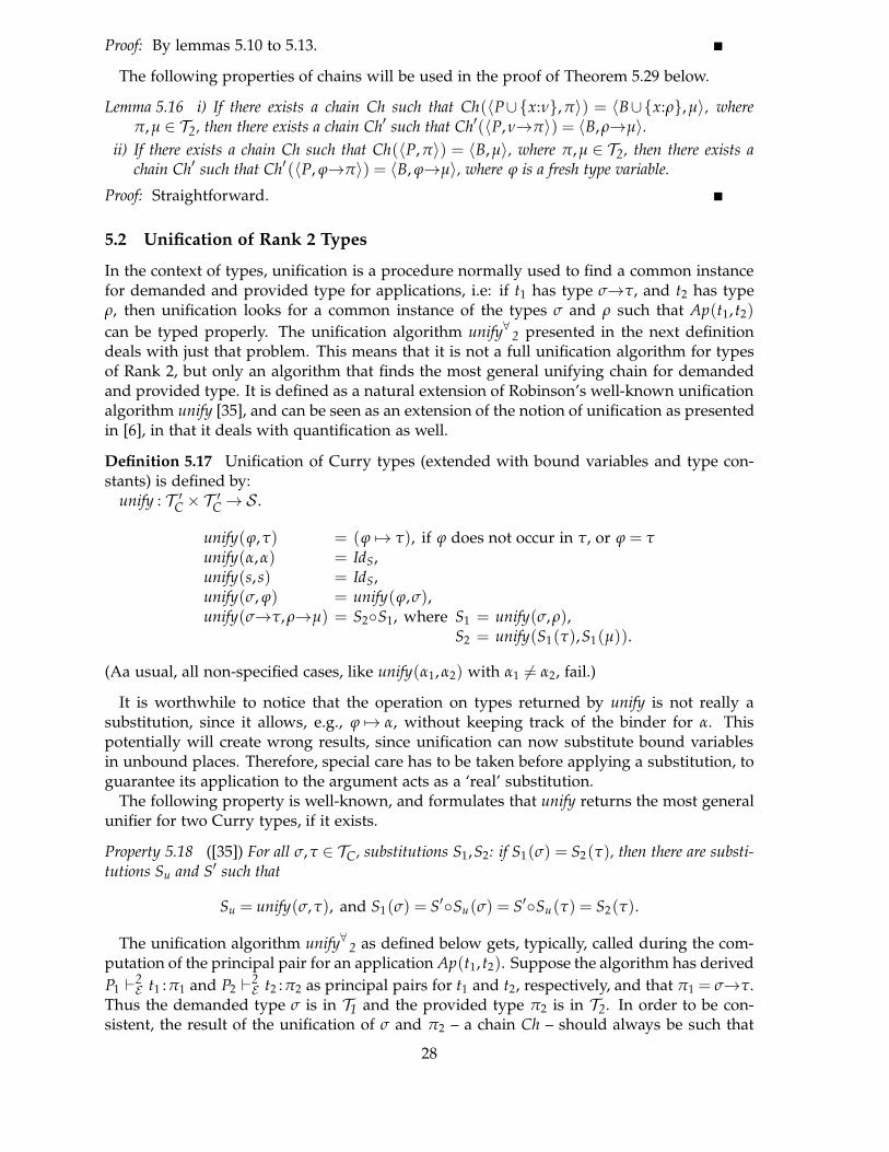
Proof: By lemmas 5.10 to 5.13.

The following properties of chains will be used in the proof of Theorem 5.29 below.

Lemma 5.16 i) If there exists a chain Ch such that Ch(〈P∪{x:ν},π〉) = 〈B∪{x:ρ},µ〉, whereπ,µ ∈ T2, then there exists a chain Ch′ such that Ch′(〈P,ν→π〉) = 〈B,ρ→µ〉.

ii) If there exists a chain Ch such that Ch(〈P,π〉) = 〈B,µ〉, where π,µ ∈ T2, then there exists achain Ch′ such that Ch′(〈P, ϕ→π〉) = 〈B, ϕ→µ〉, where ϕ is a fresh type variable.

Proof: Straightforward.

5.2 Unification of Rank 2 Types

In the context of types, unification is a procedure normally used to find a common instancefor demanded and provided type for applications, i.e: if t1 has type σ→τ, and t2 has typeρ, then unification looks for a common instance of the types σ and ρ such that Ap(t1, t2)

can be typed properly. The unification algorithm unify∀ 2 presented in the next definitiondeals with just that problem. This means that it is not a full unification algorithm for typesof Rank 2, but only an algorithm that finds the most general unifying chain for demandedand provided type. It is defined as a natural extension of Robinson’s well-known unificationalgorithm unify [35], and can be seen as an extension of the notion of unification as presentedin [6], in that it deals with quantification as well.

Definition 5.17 Unification of Curry types (extended with bound variables and type con-stants) is defined by:

unify : T ′C × T ′

C →S .

unify(ϕ,τ) = (ϕ �→ τ), if ϕ does not occur in τ, or ϕ = τunify(α,α) = IdS,unify(s, s) = IdS,unify(σ, ϕ) = unify(ϕ,σ),unify(σ→τ,ρ→µ) = S2◦S1, where S1 = unify(σ,ρ),

S2 = unify(S1(τ),S1(µ)).

(Aa usual, all non-specified cases, like unify(α1,α2) with α1 �= α2, fail.)

It is worthwhile to notice that the operation on types returned by unify is not really asubstitution, since it allows, e.g., ϕ �→ α, without keeping track of the binder for α. Thispotentially will create wrong results, since unification can now substitute bound variablesin unbound places. Therefore, special care has to be taken before applying a substitution, toguarantee its application to the argument acts as a ‘real’ substitution.

The following property is well-known, and formulates that unify returns the most generalunifier for two Curry types, if it exists.

Property 5.18 ([35]) For all σ,τ ∈ TC, substitutions S1,S2: if S1(σ) = S2(τ), then there are substi-tutions Su and S′ such that

Su = unify(σ,τ), and S1(σ) = S′◦Su(σ) = S′◦Su(τ) = S2(τ).

The unification algorithm unify∀ 2 as defined below gets, typically, called during the com-putation of the principal pair for an application Ap(t1, t2). Suppose the algorithm has derivedP1 �2

E t1 :π1 and P2 �2E t2 :π2 as principal pairs for t1 and t2, respectively, and that π1 = σ→τ.

Thus the demanded type σ is in T1 and the provided type π2 is in T2. In order to be con-sistent, the result of the unification of σ and π2 – a chain Ch – should always be such that

28

Ch(π2) ∈ T1. However, if π2 �∈ TC, then in general Ch(π2) �∈ T1. To overcome this difficulty,an algorithm toTC will be inserted that, when applied to the type ρ, returns a chain of opera-tions that removes, if possible, intersections in ρ. This can be understood by the observationthat, for example,

((σ→σ)→σ→σ)→σ is a substitution instance of ((ϕ1→ϕ1)→ϕ2)∩ (ϕ3→ϕ4→ϕ4)→ϕ5.

Note that if quantifiers appear in ρ, toTC(ρ) should fail, since quantifiers that appear beforean arrow cannot be removed by any of the operations on types.

Finally, unify∀ 2 (σ,S2(π2),S2(P2)) is called (with S2 = toTC(π2)). The basis S2(P2) is neededto calculate the expansion of S2(π2) in case σ is an intersection type.

Definition 5.19 The function toTC : T2 →S is defined by:

toTC(σ) = [IdS], if σ ∈ TCtoTC((σ1∩· · ·∩σn)→µ) = S′◦Sn, otherwise,

where Si = unify(Si−1(σ1),Si−1(σi+1))◦Si−1, (1≤ i≤n−1, with S0 = IdS), andS′ = toTC(Sn(µ))

(Again, notice that toTC(σ) fails if σ contains ‘∀’.)

The algorithm unify∀ 2 is called with the types σ and ρ′, the latter being ρ in which theintersections are removed (so ρ′ = toTC(ρ)(ρ); notice that toTC(ρ) is an operation on typesthat removes all intersections in ρ, and needs to be applied to ρ). Since none of the derivationrules, nor one of the operations, allows for the removal of a quantifier that occurs inside atype, if σ = ∀α.σ′, the unification of σ with ρ′ will not remove the ‘∀α’ part.

The following definition presents the main unification algorithm, unify∀ 2. It gets, typically,called as

unify∀ 2 (σ,S2(π2),S2(P2))

during the calculation of the principal pair for an application; after deriving P1 �2E t1 :π1 and

P2 �2E t2 :π2 as principal pairs for t1 and t2, respectively, with π1 = σ→τ and S2 = toTC(π2).

The basis is needed to calculate the expansion in case σ is an intersection type, as said above.

Definition 5.20 Let B be the set of all bases, and Ch the set of all chains. The functionunify∀2 : T ∀

C × TC ×B → Ch is defined by:

unify∀ 2 (ϕ,τ, B) = (ϕ �→ τ),

unify∀ 2 ((∀α1.σ1)∩ . . . ∩ (∀αn.σn),τ, B) = [Ex,Sn], otherwise

where Ex = n〈B,τ〉,τ1∩· · ·∩τn = Ex(τ), and

for every 1≤ i≤n, Si = unify(Si−1(σi),τi)◦Si−1 (with S0 = IdS).

It is worthwhile to notice that unify, toTC, and unify∀ 2 all return lifting-free chains. More-over, both unify and toTC return a substitution, and the chain returned by unify∀ 2 (σ,τ) actson σ as a substitution: the expansion in the chain is defined for the sake of τ only. Noticealso that unify∀ 2 does not really return a unifying chain for its first two arguments; to achievethis, also closures would have to be inserted. They are not needed for the present purpose.

The procedure unify∀ 2 fails when unify fails, and toTC fails when either unify fails or whenthe argument contains ‘∀’. Because of this relation between unify∀ 2 and toTC on one side,and unify on the other, the procedures defined here are terminating and type assignment inthe system defined in this section is decidable.

Using Property 5.18, it is possible to prove the following lemma.

29

Lemma 5.21 Let Ch be a chain.

i) If σ ∈ T2, and Ch(σ) = τ ∈ TC, then there is a S′ such that S′◦toTC(σ)(σ) = τ.ii) If σ ∈ T2, and Ch(σ) = τ ∈ T1, then there is a lifting-free chain Ch′ such that [toTC(σ)] ∗

Ch′(σ) = τ.

Proof: Easy, using Lemma 5.7(iii) and (iv).

5.3 Principal pairs for terms

In this subsection, the principal pair for a term t with respect to the environment E – ppE (t)– is defined, consisting of basis P and type π. In Theorem 5.29 it will be shown that, forevery term, this is indeed the principal one.

Notice that, in the definition below, if ppE (t) = 〈P,π〉, then π ∈ T2. For example, theprincipal pair for the term λx.x is 〈∅, ϕ→ϕ〉, so, in particular, it is not 〈∅,∀α.α→α〉. Althoughone could argue that the latter type is more ‘principal’ in the sense that it expresses thegeneric character the principal type is supposed to have, we have chosen to use the formerinstead. This is mainly for technical reasons: because unification is used in the definitionbelow, using the latter type, we would often be forced to remove the external quantifiers.Both types can be seen as ‘principal’ though, since ∀α.α→α can be obtained from ϕ→ϕ byclosure, and ϕ→ϕ from ∀α.α→α by lifting.

Definition 5.22 Let t be a term in T(F,X ). Using unify∀ 2, ppE (t) = 〈P,π〉, with π ∈ T2 isdefined by:

i) t ≡ x. Then ppE (x) = 〈{x:ϕ}, ϕ〉.ii) t ≡ λx.t′. Let ppE (t′) = 〈P,π〉, then:

a) If x occurs free in t′, and x:σ ∈ P, then ppE (λx.t′) = 〈P\x,σ→π〉.b) Otherwise, let ϕ be a fresh variable, and ppE (λx.t′) = 〈P, ϕ→π〉.

iii) t ≡ Ap(t1, t2). Let ppE (t1) = 〈P1,π1〉, ppE (t2) = 〈P2,π2〉 (choose, if necessary, trivial vari-ants such that these pairs are disjoint), and S2 = toTC(π2), then either(π1 = ϕ) : ppE (Ap(t1, t2)) = 〈P,π〉, where

P = S1(Π{P1,S2(P2)}),π = ϕ′,

S1 = (ϕ �→ S2(π2)→ϕ′), andϕ′ is a fresh variable.

(π1 = σ→τ) : ppE (Ap(t1, t2)) = 〈P,π〉, provided P and π contain no unbound occur-rences of αs, where

P = S(Π{P1,Ex(S2(P2))}),π = S(τ), and

[Ex,S] = unify∀ 2 (σ,S2(π2),S2(P2)).

iv) t ≡ F(t1, . . . , tn). Let, for every 1≤ i≤n, ppE (ti) = 〈Pi,πi〉 (choose, if necessary, trivial vari-ants such that the 〈Pi,πi〉 are disjoint in pairs), then ppE (F(t1, . . . , tn)) = 〈P,π〉, providedP and π contain no unbound occurrences of αs, where

P = Sn(Π{Ex1(S1(P1)), . . . ,Exn(Sn(Pn))},π = Sn(γ),

γ1→·· ·→γn→γ is a fresh instance of E (F),

30

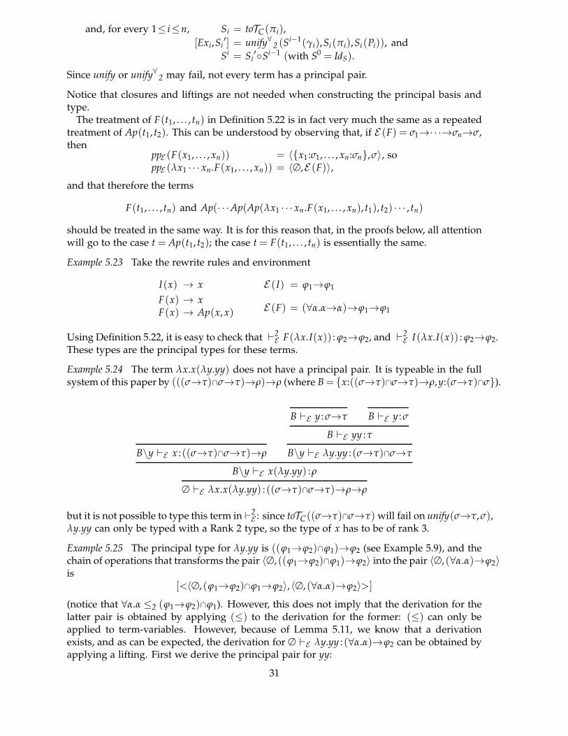
and, for every 1≤ i≤n, Si = toTC(πi),[Exi,Si

′] = unify∀ 2 (Si−1(γi),Si(πi),Si(Pi)), and

Si = Si′◦Si−1 (with S0 = IdS).

Since unify or unify∀ 2 may fail, not every term has a principal pair.

Notice that closures and liftings are not needed when constructing the principal basis andtype.

The treatment of F(t1, . . . , tn) in Definition 5.22 is in fact very much the same as a repeatedtreatment of Ap(t1, t2). This can be understood by observing that, if E (F) = σ1→·· ·→σn→σ,then

ppE (F(x1, . . . , xn)) = 〈{x1:σ1, . . . , xn:σn},σ〉, soppE (λx1 · · · xn.F(x1, . . . , xn)) = 〈∅,E (F)〉,

and that therefore the terms

F(t1, . . . , tn) and Ap(· · ·Ap(Ap(λx1 · · · xn.F(x1, . . . , xn), t1), t2) · · · , tn)

should be treated in the same way. It is for this reason that, in the proofs below, all attentionwill go to the case t = Ap(t1, t2); the case t = F(t1, . . . , tn) is essentially the same.

Example 5.23 Take the rewrite rules and environment

I(x) → xF(x) → xF(x) → Ap(x, x)

E (I) = ϕ1→ϕ1

E (F) = (∀α.α→α)→ϕ1→ϕ1

Using Definition 5.22, it is easy to check that �2E F(λx.I(x)) : ϕ2→ϕ2, and �2

E I(λx.I(x)) : ϕ2→ϕ2.These types are the principal types for these terms.

Example 5.24 The term λx.x(λy.yy) does not have a principal pair. It is typeable in the fullsystem of this paper by (((σ→τ)∩σ→τ)→ρ)→ρ (where B= {x:((σ→τ)∩σ→τ)→ρ,y:(σ→τ)∩σ}).

B\y �E x :((σ→τ)∩σ→τ)→ρ

B �E y : σ→τ B �E y :σ

B �E yy :τ

B\y �E λy.yy :(σ→τ)∩σ→τ

B\y �E x(λy.yy) :ρ

∅ �E λx.x(λy.yy) : ((σ→τ)∩σ→τ)→ρ→ρ

but it is not possible to type this term in �2E : since toTC((σ→τ)∩σ→τ) will fail on unify(σ→τ,σ),

λy.yy can only be typed with a Rank 2 type, so the type of x has to be of rank 3.

Example 5.25 The principal type for λy.yy is ((ϕ1→ϕ2)∩ϕ1)→ϕ2 (see Example 5.9), and thechain of operations that transforms the pair 〈∅, ((ϕ1→ϕ2)∩ϕ1)→ϕ2〉 into the pair 〈∅, (∀α.α)→ϕ2〉is

[<〈∅, (ϕ1→ϕ2)∩ϕ1→ϕ2〉, 〈∅, (∀α.α)→ϕ2〉>]

(notice that ∀α.α ≤2 (ϕ1→ϕ2)∩ϕ1). However, this does not imply that the derivation for thelatter pair is obtained by applying (≤) to the derivation for the former: (≤) can only beapplied to term-variables. However, because of Lemma 5.11, we know that a derivationexists, and as can be expected, the derivation for ∅ �E λy.yy : (∀α.α)→ϕ2 can be obtained byapplying a lifting. First we derive the principal pair for yy:

31

{y:(ϕ1→ϕ2)∩ϕ1} �E y : ϕ1→ϕ2 {y:(ϕ1→ϕ2)∩ϕ1} �E y : ϕ1

{y:(ϕ1→ϕ2)∩ϕ1} �E yy : ϕ2

to which we apply the lifting <〈B, ϕ2〉, 〈{y:∀α.α}, ϕ2〉> (notice that since this lifting changesonly the basis, we can actually see it as an operation on derivations):

{y:∀α.α} �E y : ϕ1→ϕ2 {y:∀α.α} �E y : ϕ1

{y:∀α.α} �E yy : ϕ2

to which we apply (→I):

{y:∀α.α} �E y : ϕ1→ϕ2 {y:∀α.α} �E y : ϕ1

{y:∀α.α} �E yy : ϕ2

∅ �E λy.yy :(∀α.α)→ϕ2

The following lemmas are needed in the proof of Theorem 5.29. The first states that if achain maps the principal pairs of terms t1, t2 in an application Ap(t1, t2) to pairs that allowthe application itself to be typed, then these pairs can also be obtained by first performing aunification. The second generalises this result to arbitrary function applications.

Lemma 5.26 Let σ ∈ T2, and for i = 1,2, ppE (ti) = 〈Pi,πi〉, such that these pairs are disjoint. LetCh1,Ch2 be chains such that

Ch1(ppE (t1)) = 〈B1,σ→τ〉, and Ch2(ppE (t2)) = 〈B2,σ〉.

Then there are a chains Chu and Chp, and type ρ ∈ T2 such that

ppE (Ap(t1, t2)) = Chu(〈Π{P1, P2},ρ〉), andChp(ppE (Ap(t1, t2))) = 〈Π{B1, B2},τ〉.

Proof: Since Ch2(π2) = σ ∈ T1, by Lemma 5.21(ii), Ch2 = Ch2 ∗ [toTC(π2)], so S2 = toTC(π2)exists; let π′

2 = S2(π2), and P′2 = S2(P2). We distinguish the cases:

(π1 = ϕ) : Then ppE (Ap(t1, t2)) = 〈S1(Π{P1, P′2}), ϕ′〉, where S1 = (ϕ �→ π′

2→ϕ′), and ϕ′ is afresh variable; take Chu = [S1,S2].

Ch1(〈P1, ϕ〉) = 〈B1,σ→τ〉, and Ch2(〈P2,π2〉) = 〈B2,σ〉.

Since π2 ∈ T2 and Ch2(π2) ∈ T1, by Lemma 5.21(ii) and Lemma 5.7(ii), there exists alifting-free chain Ch′2 such that σ = Ch′2 ∗ [S2] (π2) = Ch′2(π′

2).Also, Ch1(ϕ) = σ→τ, so there exists a chain Ch′1 such that Ch1 = Ch′1 ∗ [(ϕ �→ ϕ1→ϕ2)],

so such that Ch′1(ϕ1) = σ, and Ch′1(ϕ2) = τ.Since Ch1(π1) = σ = Ch′2 ∗ [S1,S2] (π2), in particularTo show: there exists Chp such that Chp(ppE (Ap(t1, t2))) = 〈Π{B1, B2},τ〉, so such that

Chp(〈S1(Π{P1, P′2}), ϕ′〉) = 〈Π{B1, B2},τ〉.

(π1 = µ1→µ2) : Notice that Ch1(π1) = Ch1(µ1→µ2) = σ→τ ∈ T2, so, by Lemma 5.7(v), thereare substitution S, and lifting L such that

Ch1(π1) = [S,L] (π1).

32

So there are B′ ≥ B, σ ≤ ρ1, ρ2 ≤ τ such that

S(π1) = S(µ1→µ2) = ρ1→ρ2, (So S(µ1) = ρ1), andL = <〈B′,ρ1→ρ2〉, 〈B,σ→τ〉>.

In particular,

π1 = µ1→µ2, so (µ1 ∈ T1,µ2 ∈ T2)π1 = (∀α1.δ1∩ · · · ∩∀αm.δm)→ µ2, so (δj ∈ TC (1≤ j≤m), µ2 ∈ T2)

S(π1) = (∀α1.S(δ1)∩ · · · ∩∀αm.S(δm))→ S(µ2) = ρ1→ρ2.

Notice that <〈B,σ〉, 〈B,ρ1〉> is a lifting, and Ch2 ∗ [<〈B,σ〉, 〈B,ρ1〉>] (π2) = ρ1 ∈ T1.Then, by Lemma 5.21(ii), there is a lifting-free chain Ch′ such that Ch′(π′

2) = ρ1. Then

Ch′ = [Ex′,S′,Cl], with Ex′(π′2) = S′

1(π′2)∩ · · · ∩S′

n(π′2), (∀ free)

[Ex′,S′] (〈P′2,π′

2〉) = 〈B1,ν〉, with ν = S′(S′1(π

′2))∩ · · · ∩S′(S′

n(π′2)), ”

Cl(〈B,ν〉) = 〈B,ρ1〉, with ρ1 = ∀α1.ν12∩ · · · ∩∀αm.νm

2

So, for 1≤ j≤m, S(δj) = νj2 = S′(S′

j(π′2)), and, by Property 5.18, there exists substitutions

Sju,Sj such that

Sju = unify(δj,π′

2)

S(δj) = Sj(Sju(δj)) = ν

j2 = Sj(Sj

u(π′2)) = S′(S′

j(π′2))

Since the substitutions Sju agree on type-variables, without loss of generality, we can

assume that exists substitutions S1, . . . ,Sm such that

Si = unify(Si−1(δi),π′2)◦Si−1 (with S0 = IdS), and

for 1≤ j≤m, Sj(Sn(δj)) = νj2 = Sj(Sn(π′

2))

so, by Definition 5.20

Ch′u = unify∀ 2 ((∀α1.δ1)∩ . . . ∩ (∀αn.δn),π′2, P′

2).

exists. Take Chu = [S2] ∗ Ch′u, Chp = [S1◦ · · · ◦Sm,<〈B,ρ2〉, 〈B,τ〉>], and ρ = µ2.Notice that, since B can be assumed to not contain free occurrences of αs, the last chain iswell-defined.

Lemma 5.27 Let σ ∈ T2, and, for every 1≤ i≤n, ppE (ti) = 〈Pi,πi〉, such that the pairs 〈Pi,πi〉 andthe type E (F) = γ1→·· ·→γn→γ are disjoint, and let Ch(F),Ch1, . . . ,Chn be chains such that

ChF(E (F)) = σ1→·· ·→σn→σ and, for every 1≤ i≤n,Chi(〈Pi,πi〉) = 〈Bi,σi〉.

Then there are chains Chg and Chp such that

ppE (F(t1, . . . , tn)) = Chg(〈Π{P1, . . . , Pn},γ〉), andChp(ppE (F(t1, . . . , tn))) = 〈Π{B1, . . . , Bn},σ〉.

Proof: This is a generalisation of the proof of the previous lemma.

The main result of this section then becomes the soundness and completeness result forppE .

Theorem 5.28 (Soundness of ppE ) If ppE (t) = 〈P,π〉, then P �2E t :π.

33

Proof: By induction on the structure of terms.(t ≡ x) : Since ppE (x) = 〈{x:ϕ}, ϕ〉, the result follows from rule (≤2).(t ≡ λx.t′) : a) If x occurs free in t′, then there are σ,π such that ppE (λx.t′) = 〈P,σ→π〉,

where ppE (t′) = 〈P, x:σ , π〉. By induction, P, x:σ �2E t′ :π, and, by applying rule

(→I), also P �2E λx.t′ :σ→π.

b) Otherwise, there are ϕ,π such that ppE (λx.t′) = 〈P, ϕ→π〉, where ppE (t′) = 〈P,π〉,with ϕ a fresh variable. By induction, P �2

E t′ :π. Since x does not occur in P,we have P, x:ϕ ≤2 P, and P, x:ϕ �2

E t′ :π by Lemma 5.11, and then, by rule (→I),P �2

E λx.t′ : ϕ→π.(t ≡ Ap(t1, t2)) : Then there are P1, P2 such that ppE (t1) = 〈P1,π1〉, ppE (t2) = 〈P2,π2〉, and, by

induction, P1 �2E t1 :π1 and P2 �2

E t2 :π2. Notice that, by construction, the two principalpairs share no type variables. Let S2 = toTC(π2). Then either:(π1 = ϕ) : Then ppE (Ap(t1, t2)) = 〈S1(Π{P1,S2(P2)}), ϕ′〉, where S1 = (ϕ �→ S2(π2)→ϕ′),

and ϕ′ is a fresh variable. Let S = S1◦S2, then, by Lemma 5.10,

S(P1) �2E t1 :S(π1) and S(P2) �2

E t2 :S(π2).

We know that S(π1) = S1(ϕ) = S2(π2)→ϕ′. Since S2 has no effect on P1, S(Π{P1, P2}) =S1(Π{P1,S2(P2)}). Also, since S1 does not affect any variable in S2(〈P2,π2〉), wehave S(P2) = S2(P2), and S(π2) = S2(π2). So, by rule (→E), S(Π{P1, P2}) �2

E Ap(t1, t2) : ϕ′.(π1 = σ→τ, with σ ∈ T1, τ ∈ T2) : Then ppE (Ap(t1, t2)) = 〈S(Π{P1,Ex(S2(P2))}),S(τ)〉,

where [Ex,S] = unify∀ 2 (σ,S2(π2),S2(P2)). Let Ch = [S2,Ex,S], then, by Lemma 5.15,

Ch(P1) �2E t1 :Ch(π1) and Ch(P2) �2

E t2 :Ch(π2).

Since [Ex,S] (σ) = [Ex,S] (S2(π2)), and S2 has no effect on 〈P1,σ→τ〉, we have Ch(σ) =Ch(π2) and S(Π{P1,Ex(S2(P2))}) = Ch(Π{P1, P2}). Also, since the chain returnedby unify∀ 2 acts on 〈P1,σ→τ〉 as a substitution, we get Ch(σ→τ) = Ch(π2)→S(τ).But then, by rule (→E), Ch(Π{P1, P2}) �2

E Ap(t1, t2) :S(τ).(t ≡ F(t1, . . . , tn)) : As the previous part, using that the fresh instance of the environment

type for F is can be used for F here (see the proof of Lemma 5.10).

Theorem 5.29 (Completeness of ppE ) If B �2E t :σ, then there are a basis P and type π such that

ppE (t) = 〈P,π〉, and there is a chain Ch such that Ch(〈P,π〉) = 〈B,σ〉.Proof: By induction on the structure of derivations.(≤2) : Then t ≡ x, σ ∈ TC, and there is τ ∈ T1 such that x:τ ∈ B and τ ≤2 σ. Also, π = ϕ

and P = {x:ϕ}. Since τ ≤2 σ, B ≤2 {x:σ}, so <〈{x:σ},σ〉, 〈B,σ〉> is a lifting. Take Ch =[ϕ �→ σ,<〈{x:σ},σ〉, 〈B,σ〉>].

(∩I) : Then σ = σ1∩· · ·∩σn, and, for 1≤ i≤n, B �2E t :σi, with σi ∈ T ∀

C. Let ppE (t) = 〈P,π〉,and let Ex = n〈P,π〉, then Ex(〈P,π〉) = 〈Π{P1, . . . , Pn},π1∩ · · · ∩πn〉, with each pair 〈Pi,πi〉a trivial variant of 〈P,π〉. So, without loss of generality, we can even say ppE (t) = 〈Pi,πi〉,for all 1≤ i≤n. By induction, there exist chains Ch1, . . . ,Chn such that for 1≤ i≤n,Chi(〈Pi,πi〉) = 〈B,σi〉. By Lemma 5.7(ii), Chi = [Si,Cli]. Take Ch= [Ex,S1◦ · · · ◦Sn,Cln, . . . ,Cln].

(→I) : Then t ≡ λx.t′, and there are ρ,µ such that σ = ρ→µ, and B, x:ρ �2E t′ :µ. Let ppE (t′) =

〈P′,π′〉, then(x ∈ FV(t′)) : Let x:ν ∈ P′, then P = P′\x, and ppE (λx.t′) = 〈P,ν→π′〉. By induction

there exists a chain Ch′ such that

Ch′(〈P, x:ν , π′〉) = 〈B, x:ρ , µ〉.34

Then, by Lemma 5.16(i), there exists a chain Ch′′ such that Ch′′(〈P,ν→π′〉) = 〈B,ρ→µ〉.Take Ch = Ch′′.

(x �∈ FV(t′)) : Then ppE (λx.t′) = 〈P′, ϕ→π′〉, where ϕ is a type-variable not occurringin any other type. By induction there exists a chain Ch′ such that Ch′(〈P,π〉) =〈B,µ〉. Then, by Lemma 5.16(ii), there exists a chain Ch′′ such that Ch′′(〈P, ϕ→π〉) =〈B, ϕ→µ〉. Let Ch′′ = [Ex,S,L,Cl], then take Ch = [Ex,S◦(ϕ �→ ρ),L,Cl].

(→E) : Then t ≡ Ap(t1, t2), and there is a τ ∈ T2 such that B �2E t1 :τ→σ, and B �2

E t2 :τ. Byinduction, for i = 1, 2, there are Pi,πi, and chain Chi such that

ppE (ti) = 〈Pi,πi〉, Ch1(ppE (t1)) = 〈B,τ→σ〉, and Ch2(ppE (t2)) = 〈B,τ〉.

Then, by Lemma 5.26, there is a chain Ch such that Ch(ppE (Ap(t1, t2))) = 〈B,σ〉.(∀ I) : Then σ = ∀α.τ[α/ϕ], and B �2

E t :τ. Let ppE (t) = 〈P,π〉, then by induction there existsa chain Ch′ such that Ch′(〈P,π〉) = 〈B,τ〉. Take Cl = 〈τ, ϕ〉, and Ch = Ch′ ∗ [Cl].

(F ) : Then t ≡ F(t1, . . . , tn). There are σ1, . . . ,σn such that, for every 1≤ i≤n, B �2E ti :σi, and

a chain ChF such that ChF(E (F)) = σ1→·· ·→σn→σ. By induction, for 1≤ i≤n, there are〈Pi,πi〉, (disjoint in pairs) and a chain Chi, such that

ppE (ti) = 〈Pi,πi〉, and Chi(ppE (ti)) = 〈B,σi〉.

Since the pairs 〈Pi,πi〉 are disjoint, the chains Chi do not interfere. Assume, withoutloss of generality, that none of the type-variables occurring in E (F) occur in any of thepairs 〈Pi,πi〉. Then, by Lemma 5.27, there is a chain Ch such that Ch(ppE (F(t1, . . . , tn))) =〈B,σ〉.

6 Conclusions

In this paper we made a further step inside the partially unexplored field of type assignmentsystems for term rewriting systems extended with abstraction and β-rule. Various extensionsof term rewriting containing the notions of abstraction and β-rule have been intensivelyexplored in the last decade in a plethora of papers leaving, however, the concept of typeassignment in such a context still partially in darkness. We believe that if the study ofthe combined computational paradigm Lambda Calculus and Algebraic Rewriting can beof help not only for the development of interactive proof assistant tools, but also as basisfor powerful and expressive programming languages, the topic of type systems, and typeassignment systems in particular, cannot be left unattended. We have focused on a typeassignment aiming a being both powerful, by using intersection types, and expressive, byadding the universal type quantification.

We cannot help to sympathize with the reader who had to go through the heavy techni-calities that the notion of intersection types brings, particularly when connected with termrewriting and universal quantification. But this has not to leave the impression of a useless-ness of the sort of type assignment we propose. The typing power of our general system issuch to leave space to many kind of restrictions, needed also because of its undecidability.As a matter of fact, we proposed a decidable restriction which, besides having such feature,gets rid of many technicalities of the general system. We do not claim such restriction to be”the restriction” for a practical use of the proposed notion of type assignment for LambdaCalculus + Algebraic Rewriting, but simply wished to show one possibility.

The present paper then aims at being the theoretical platform from which we can start forfurther investigations, which will be focused on restricted versions of the general system.One other question to be addressed, directly in the context of some restricted version, is

35

if the proposed notion of type assignment easily extends to other type constructors oftenused in actual type system for programming languages (e.g. the polymorphic lists or therestriction to type classes of the language Haskell).

Acknowledgements

The second author would like to thank Mariangiola Dezani and Carmelo Dell’Acqua for allthey taught him in different fields.

References

[1] Z. Ariola, R. Kennaway, J.W. Klop, R. Sleep, and F-J. de Vries. Syntactic definitions of undefined:on defining the undefined. In M. Hagiya and J.C. Mitchell, editors, Proceedings of TACS ’94.International Symposium on Theoretical Aspects of Computer Software, Sendai, Japan, volume 789 ofLecture Notes in Computer Science, pages 543–554. Springer-Verlag, 1994.

[2] S. van Bakel. Complete restrictions of the Intersection Type Discipline. Theoretical ComputerScience, 102(1):135–163, 1992.

[3] S. van Bakel. Partial Intersection Type Assignment in Applicative Term Rewriting Systems. InM. Bezem and J.F. Groote, editors, Proceedings of TLCA ’93. International Conference on Typed LambdaCalculi and Applications, Utrecht, the Netherlands, volume 664 of Lecture Notes in Computer Science,pages 29–44. Springer-Verlag, 1993.

[4] S. van Bakel. Principal type schemes for the Strict Type Assignment System. Logic and Computa-tion, 3(6):643–670, 1993.

[5] S. van Bakel. Intersection Type Assignment Systems. Theoretical Computer Science, 151(2):385–435,1995.

[6] S. van Bakel. Rank 2 Intersection Type Assignment in Term Rewriting Systems. FundamentaInformaticae, 2(26):141–166, 1996.

[7] S. van Bakel, F. Barbanera, and M. Fernandez. Rewrite Systems with Abstraction and β-rule:Types, Approximants and Normalization. In Hanne Riis Nielson, editor, Programming Languagesand Systems – ESOP’96. Proceedings of 6th European Symposium on Programming, Linkoping, Swe-den, volume 1058 of Lecture Notes in Computer Science, pages 387–403. Springer-Verlag, 1996.

[8] S. van Bakel and M. Fernandez. Normalization Results for Typeable Rewrite Systems. Informationand Computation, 133(2):73–116, 1997.

[9] F. Barbanera and M. Fernandez. Intersection Type Assignment Systems with Higher-Order Al-gebraic Rewriting. TCS, 170:173–207, 1996.

[10] F. Barbanera, M. Fernandez, and H. Geuvers. Modularity of Strong Normalization and Con-fluence in the Algebraic λ-cube. In Proceedings of the ninth Annual IEEE Symposium on Logic inComputer Science, Paris, France, 1994.

[11] H. Barendregt. The Lambda Calculus: its Syntax and Semantics. North-Holland, Amsterdam, revisededition, 1984.

[12] H. Barendregt, M. Coppo, and M. Dezani-Ciancaglini. A filter lambda model and the complete-ness of type assignment. Journal of Symbolic Logic, 48(4):931–940, 1983.

[13] V. Breazu-Tannen. Combining algebra and higher-order types. In Proceedings of the Third AnnualIEEE Symposium on Logic in Computer Science, pages 82–90, 1988.

[14] V. Breazu-Tannen and J. Gallier. Polymorphic rewriting conserves algebraic strong normalization.Theoretical Computer Science, 83(1):3–28, 1991.

[15] V. Breazu-Tannen and J. Gallier. Polymorphic rewriting conserves algebraic confluence. Informa-tion and Computation, 82:3–28, 1992.

[16] A. Bucciarelli, S. De Lorenzis, A. Piperno, and I. Salvo. Some computational properties of in-tersection types (extended abstract). In Proc. Symposium on Logic in Computer Science (LICS’99),pages 109–118, 1999.

36

[17] L.M.M. Damas. Type Assignment in Programming Languages. PhD thesis, University of Edinburgh,Department of Computer Science, Edinburgh, 1985. Thesis CST-33-85.

[18] N. Dershowitz and J.P. Jouannaud. Rewrite systems. In J. van Leeuwen, editor, Handbook ofTheoretical Computer Science, volume B, chapter 6, pages 245–320. North-Holland, 1990.

[19] D. J. Dougherty. Adding algebraic rewriting to the untyped lambda calculus. Information andComputation, 101:251–267, 1992.

[20] M. Fernandez. Type Assignment and Termination of Interaction Nets. Mathematical Structures ofComputer Science, 1998.

[21] M. Fernandez and J.P. Jouannaud. Modular termination of term rewriting systems revisited. InE. Astesiano and A. Tarlecki, editors, Recent Trends in Data Type Specification. 10th Workshop onSpecification of Abstract Data Types, S. Margherita, Italy, volume 906 of Lecture Notes in ComputerScience, pages 255–272. Springer-Verlag, 1994.

[22] J.-Y. Girard, Y. Lafont, and P. Taylor. Proofs and Types. Cambridge Tracts in Theoretical ComputerScience. Cambridge University Press, 1989.

[23] J.Y. Girard. The System F of Variable Types, Fifteen years later. Theoretical Computer Science,45:159–192, 1986.

[24] B. Jacobs, I. Margaria, and M. Zacchi. Filter models with polymorphic types. Theoretical ComputerScience, 95:143–158, 1992.

[25] T. Jim. What are principal typings and what are they good for? In Proceedings 23th ACMSymposium on Principles of Programming Languages, 1996.

[26] J.P. Jouannaud and M. Okada. Executable higher-order algebraic specification languages. InProceedings of the Sixth Annual IEEE Symposium on Logic in Computer Science, pages 350–361, 1991.

[27] A.J. Kfoury and J. Tiuryn. Type reconstruction in finite-rank fragments of the second-order λ-calculus. Information and Computation, 98(2):228–257, 1992.

[28] A.J. Kfoury and J. Wells. A Direct Algorithm for Type Inference in the Rank-2 Fragment of theSecond-Order λ-Calculus. In LFP’94, 1994.

[29] A.J. Kfoury and J.B. Wells. Principality and decidable type inference for finite-rank intersectiontypes. In Proceedings 26th ACM Symposium on Principles of Programming Languages, pages 161–174,1999.

[30] J.W. Klop. Term Rewriting Systems. In S. Abramsky, Dov.M. Gabbay, and T.S.E. Maibaum,editors, Handbook of Logic in Computer Science, volume 2, chapter 1, pages 1–116. Clarendon Press,1992.

[31] J. Launchbury and S.L. Peyton Jones. Lazy functional state threads. In Proc. ACM SIGPLAN’94Conference on Programming Language Design and Implementation, 1994.

[32] I. Margaria and M. Zacchi. Principal Typing in a ∀ ∩ -Discipline. Logic and Computation, 5(3):367–381, 1995.

[33] M.H.A. Newman. On theories with a combinatorial definition of ‘equivalence’. Ann. Math.,43:223–243, 1942.

[34] E.G.J.M.H. Nocker, J.E.W. Smetsers, M.C.J.D. van Eekelen, and M.J. Plasmeijer. Concurrent Clean.In Proceedings of PARLE ’91, Parallel Architectures and Languages Europe, Eindhoven, The Nether-lands, volume 506-II of Lecture Notes in Computer Science, pages 202–219. Springer-Verlag, 1991.

[35] J.A. Robinson. A machine-oriented logic based on the resolution principle. Journal of the ACM,12(1):23–41, 1965.

[36] S. Ronchi Della Rocca and B. Venneri. Principal type schemes for an extended type theory.Theoretical Computer Science, 28:151–169, 1984.

[37] H. Yokohuchi. Embedding a Second-Order Type System into an Intersection Type System. Infor-mation and Computation, 117:206–220, 1995.

37

Appendix

Property 3.9 Let B �E t :σ, where B = {x1:σ1, . . . , xn:σn}, and let FV(σ1, . . . ,σn,σ) ⊆ {ϕ}.Then, given a sequence of types γ such that |γ| = |ϕ| and a sequence of reducibility candi-dates Rγ, if R is a term-substitution that is Rγ-reducible for B, then tR ∈ Red σ[Rγ/ϕ].

Proof: By Notherian induction on ‘�SN’. If σ ≡ σ1∩· · ·∩σn, then, by definition, we haveto prove that, for any 1≤ i≤n, tR ∈ Red σi [Rγ/ϕ]. Thus, without loss of generality we canconsider σ not to be an intersection.

Let γ and Rγ be as in the hypothesis of the property and let R = {x1 �→ u1, . . . , xn �→ un}.We distinguish the cases:

i) t is a neutral term. If t is a variable xj, then we have necessarily that σj ≤ σ. Since R is Rγ-reducible for B, xjR ∈ Red τ[Rγ/ϕ], and, by Lemma 3.6, we have also that xjR ∈ Red σ[Rγ/ϕ].So, without loss of generality we can assume that t is not a variable. This impliesthat also tR is neutral. If tR is irreducible, then tR ∈ Red σ[Rγ/ϕ] holds by (C3). Oth-erwise, let tR → t′ at position p. We will prove either tR ∈ Red σ[Rγ/ϕ] itself, or provet′ ∈ Red σ[Rγ/ϕ] and apply (C3).

a) p = qp′, where t|q ≡ xi ∈ X . So the redex is in a sub-term of tR that is introduced bythe term-substitution. Let z be a new variable.

Take now R′ such that R′ = R ∪ {z �→ t′ |q}. Note that tR|q → t′|q at position p′.Since tR|q ∈ {R} and R is assumed to be Rγ-reducible for B, also tR|q ∈ Red σi [Rγ/ϕ]

holds. So, by (C2) we have that also t′ |q ∈ Red σi [Rγ/ϕ] holds. Then we have that R′

is Rγ-reducible for B,z:σi.Now, if the variable xi (≡ t|q) has exactly one occurrence in t, then t ≡ t[z]q modulo

renaming of variables. Otherwise, t>· t[z]q . In the first case (since R contains a termthat is rewritten to get R′) we have I(tR) �SN

3 I(t[z]R′q ), and I(tR) �SN

2 I(t[z]R′q )

in the second case. Both cases yield, by induction, t[z]R′

q ∈ Red σ[Rγ/ϕ]. Note that

t[z]R′

q ≡ t′.b) Now assume that p is a non-variable position in t. We analyze separately the cases:

1) p is not the root position. Note that t|pR ≡ tR|p. Let τk (k ∈ K) be a type assignedto t|p in the derivation of B �E t : σ, then

tR|p ∈ Red τk [Rγ/ϕ] (1)

holds by induction. Let z be a new variable, and take R′ such that R′ = R ∪{z �→ tR|q}. By (1), and since

Red⋂

k ∈ K τk [Rγ/ϕ] ≡⋂

k ∈ K

Red τk [Rγ/ϕ],

R′ is reducible for B ∪ {z:⋂

k ∈ K τk}. Moreover B ∪ {z:⋂

k ∈ K τk} �E t[z]p :σ. Now,since, t>· t[z]p, we have that I(tR) �SN

2 I(t[z]R′p ), and hence tR ∈ Red σ[Rγ/ϕ]

because tR ≡ t[z]R′

p and, by induction, t[z]R′

p ∈ Red σ[Rγ/ϕ].2) p is the root position. Then the possible cases for t are:

A) t ≡ F(t1 . . . tn), where at least one of the ti’s is not a variable, and F is ei-ther a defined symbol of arity n, or F ≡ Ap and n = 2. Take now z1, . . . ,znnew variables and R′ such that R′ = R ∪ {z1 �→ t1R, . . . ,zn �→ tnR}. Since t>· ti,I(tR) �SN

2 I(tiR). Then if B �E ti :ξi, tiR ∈ Red ξi [Rγ/ϕ] holds by induction,

38

and hence R′ is Rγ-reducible for B ∪ {z1:ξ1, . . . ,zn :ξn}. Since t>· F(z1, . . . ,zn),we have I(tR)�SN

2 I(F(z1, . . . ,zn)R′). Now, F(z1, . . . ,zn)R′ ≡ tR and

B ∪ {z1:ξ1, . . . ,zn :ξn} �E F(z1, . . . ,zn) :σ.

Hence, by induction, tR ∈ Red σ[Rγ/ϕ].B) t ≡ Fk(z1, . . . ,zn) where z1, . . . ,zn are different variables. (If zi ≡ zj for some

i �= j, we can reason as in the case above, taking z′1, . . . ,z′n, new pair-wisedistinct variables, and R′ = {z′1 �→ z1R, . . . ,z′n �→ znR}.) Then tR must be aninstance of the left-hand side of a rule defining Fk, that is a rule of the form

Fk(C[x],y)→ C′ [Fk(C1x],y), . . . , Fk(Cm [x],y),y].

Therefore we have

tR ≡ Fk(z1, . . . ,zn)R

≡ Fk(C[v],w)→ C′ [Fk (C1v,w), . . . , Fk(Cm [v],w),w]≡ t′,

where C[v],w are all terms in {R}, and hence, by hypothesis, for suitable i’s,they belong to Red σi [Rγ/ϕ]. Now we will deduce t′ ∈ Red σ[Rγ/ϕ] in threesteps:

(Step I) : Let R′ be the term-substitution that maps Fk(C[x],y) to Fk(C[v],w) ≡ tR.By the definition of the general scheme, x ⊆ y and hence v ⊆ w. Then,since w are terms in {R}, by hypothesis we have w ∈ Red σ1[Rγ/ϕ], whereσ1 ⊆ σ. We can then infer that v ∈ Redσ2[Rγ/ϕ], where σ2 ⊆ σ1.Take a derivation for our term Fk(C[v],w). Let ρv be the types given to vin the derivation. Now, by Subject Reduction (Theorem 2.27) it is easy tocheck that, for every 1≤ j≤m and 1 ≤ k′ ≤ |C| it is possible to type Cj′k

[x]from the basis {x:ρv}. We can show that R′ is Rγ-reducible for {x:ρv}, asfollows:Consider a derivation for the principal pair of the left hand side of the rule:

y:µ, . . . �E Fk(C[x],y) :µ′

and assume that E(Fk) = µ1→·· ·→µn→σ. Note that by the definitionof the general scheme, the types appearing in the principal basis for thearguments y of Fk are the types required by E(Fk). All the types τ used forx ⊆ y in this derivation satisfy µ ≤ τ. Any valid derivation for an instanceof the left-hand side can be obtained by a chain of operations applied tothe principal one, in particular the derivation that assigns the types ρ tothe occurrences of x in C[x] and σ2 to the occurrences of x in y. Hence,there is a chain of operations that transforms µ into σ2 and τ into ρ. Recallthat substitution and expansions preserve the ≤ relation on types. Liftingand closure can transform µ or its instances into smaller types, hence, stillsmaller than τ. In this way we can build a derivation for Fk(C[v],w) wherethe types ρv assigned to v are such that σ2 ≤ ρv. Now, by Lemma 3.6, wehave v ∈ Redρv[Rγ/ϕ], that is R′ is Rγ-reducible for {x:ρv}1.

1 With the version of the scheme that does not require v ⊆ w but assumes that the terms in v that do notappear in w are assigned base types, we can deduce that R′ is reducible because SN (v).

39

For every 1≤ j≤m, Fk does not occur in C[ j] (by definition of the general

scheme), hence for every 1 ≤ k′ ≤ |C[ j]|, I(Fk(z1, . . . ,zn)R)�SN1 I(Cj′k

[x]R′).

Now, since R′ is Rγ-reducible for {x:ρv}, it is possible to apply the induc-

tion hypothesis obtaining Cj′k[x]R

′∈ Red τjk′ [Rγ/ϕ] for any type τjk′ we can

give to Cj′k[x] from the basis {x:ρv}. In particular when τj1→ . . .→τjn→σj

is the type used for Fk in the sub-derivation for the right hand side of ourreduction rule having Fk(Cj [x],w) as the subject of the conclusion.

(Step II) : Let, for 1≤ j≤m, Rj be the term-substitution such that

Fk(z1, . . . ,zc,y)Rj ≡ Fk(Cj [v],w) ≡ Fk(Cj [x],w)R′

(c = |C|). By (Step I), Rj is Rγ-reducible for

B′ = {z1:τj1 , . . . ,zcj :τjcj,y:σ1},

where σ1 ⊆ σ. Since C>mulC[ j], and > is closed under term-substitution,

also CR′>mulC[ j]

R′

. So I(Fk(z1, . . . ,zn)R) �SN3 I(Fk(z1, . . . ,zcj ,y)

Rj), andtherefore, by induction, Fk(z1, . . . ,zcj ,w)

Rj ∈ Red σj [Rγ/ϕ].(Step III) : Let v be the term obtained by replacing, in the right-hand side of the rule,

the terms Fk(C1v,w), . . . , Fk(Cm [v],w) by fresh variables z′1, . . . ,z′m, that is,v = C′ [z′1, . . . ,z′m,y]. Let R′′ be the term-substitution such that

vR′′≡ C′ [Fk(C1v,w), . . . , Fk(Cm [v],w),w],

then tR → vR′′. Notice that, by (Step II), R′′ is Rγ-reducible for the ba-

sis B′′ = {z′1:σ1, . . . ,z′m:σm,y:σ1}, where σ1 ⊆ σ. When an Fj occurs in vthen, by the general scheme, j < k and, therefore, I(Fk(z1, . . . ,zn)R) �SN

1

I(vR′′). Hence, vR′′ ∈ Red σ[Rγ/ϕ], by induction. Since t′ ≡ vR′′

, we gett′ ∈ Red σ[Rγ/ϕ].

C) t ≡ Ap(z1,z2) where z1,z2 ∈ X . We prove this part by induction on the struc-ture of the derivation for B �E Ap(z1,z2) :σ.

(≤), (F ) : Not applicable.(→E) : Then there is a τ such that B �E z1 :τ→σ and B �E z2 :τ. Then, by rule

(≤), there are ρ1,ρ2 such that {z1:ρ1,z2:ρ2} ⊆ B, ρ1 ≤ τ→σ, and ρ2 ≤ τ.Since z1R and z2R are Rγ-reducible in B, we have z1R ∈ Red ρ1 [Rγ/ϕ], andz2R ∈ Red ρ2 [Rγ/ϕ]. Then, by Lemma 3.6, also z1R ∈ Red τ→σ[Rγ/ϕ], andz2R ∈ Red τ[Rγ/ϕ]. Then, by Definition 3.3, Ap(z1R,z2R) ∈ Red σ[Rγ/ϕ].Notice that Ap(z1R,z2R) is the same as Ap(z1,z2)R.

(∩I) : Then σ ≡ τ1∩· · ·∩τm. The thesis follows easily by induction, since

Red τ1∩···∩τm [Rγ/ϕ] ≡ Red τ1 [Rγ/ϕ]∩ · · · ∩ Red τm [Rγ/ϕ].

(∀E) : Then σ ≡ σ′[τ/ϕ′] where the type in the premise of the rule is ∀ϕ′.σ′. Since∀ϕ′.σ′ ≤ σ′[τ/ϕ′], the result follows by induction and Lemma 3.6.

(∀ I) : Then σ ≡ ∀ϕ′.σ′ and B �E t : σ′. Moreover, ϕ′ �∈ FV(σ1, . . . ,σn). By induc-tion, for any sequence of types γ,δ such that |γ,δ| = |ϕ, ϕ′| and any se-quence of reducibility candidates Rγ,Sδ: if R is a term-substitution Rγ,Sδ-reducible for B, then tR ∈ Red σ′

[Rγ/ϕ,Sδ/ϕ′]. Since ϕ′ �∈ FV(σ1, . . . ,σn), itfollows that, for any 1≤ j≤n,

Red σj [Rγ/ϕ,Sδ/ϕ′] ≡ Red σj [Rγ/ϕ].

40

This means that a term-substitution which is Rγ,Sδ-reducible for B, is alsoRγ-reducible for B. Hence we can restate the induction hypothesis as fol-lows: for any sequence of types γ such that |γ| = |ϕ| and any sequence ofreducibility candidates Rγ, if R is a term-substitution Rγ-reducible for B,then for any type δ and reducibility candidate Sδ, tR ∈ Red σ′

[Rγ/ϕ,Sδ/ϕ′].By definition of reducibility candidates this means that Ap(z1,z2)R ∈ Red∀ ϕ′.σ′

[Rγ/ϕ].ii) t is not neutral. Let t ≡ λx.u.

We can proceed by induction on the structure of the derivation of B �E λx.u :σ. Theargument is similar to that used for the case t ≡ Ap(z1,z2). We prove only the interestingpart, when the last rule is (→I), and σ ≡ ρ→β. Then we need to show that, given v suchthat v ∈ Red ρ[Rγ/ϕ], we have that Ap(tR,v) ∈ Red β[Rγ/ϕ]. Since the term Ap(tR,v) isneutral, by (C3) it is enough to prove t′ ∈ Red β[Rγ/ϕ] for all t′ such that Ap(tR,v)→ t′.This will be proved by induction on the sum of the length of the rewrite sequences outof v and out of R. Note that since v and R are reducible, by (C1) SN (v) and SN (R).(Base) : If v and R are in normal form, the only reduction step out of Ap(tR,v) can be:

Ap((λx.u)R,v)→ t′ ≡ uR′,

where R′ ≡ R ∪ {x �→ v}. R′ is reducible because v ∈ Red ρ[Rγ/ϕ]. Now, since(λx.u)>· u, I(λx.uR) �SN

2 I(uR′). By induction we have uR′ ∈ Red β[Rγ/ϕ]. Note

that uR′ ≡ t′.(Induction step) : Otherwise, the reduction step out of Ap(tR,v) must take place inside

v or R. Then t′ is computable by induction.

41