Part I Informal Presentationjbw/papers/Wells+Haack:Branching...Branching Types J. B. Wellsy...

Branching Types∗

J. B. Wells† Christian Haack

2002-08-18

Abstract

Although systems with intersection types have many unique capabilities, there has

never been a fully satisfactory explicitly typed system with intersection types. We

introduce and prove the basic properties of λB, a typed λ-calculus with branching types

and types with quantification over type selection parameters. The new system λB is

an explicitly typed system with the same expressiveness as a system with intersection

types. Typing derivations in λB use branching types to squash together what would be

separate parallel derivations in earlier systems with intersection types.

Part I

Informal Presentation

This part presents our new system λB and its motivation and implications in a way thatwe hope is understandable yet without requiring too many technical details. The technicalpresentation and formal statements are deferred to part II.

1 Background and Motivation

1.1 Intersection Types

Intersection types were independently invented near the end of the 1970s by Coppo andDezani [CDC80] and Pottinger [Pot80]. Intersection types provide type polymorphism bylisting type instances, differing from the more widely used ∀-quantified types [Gir72, Rey74],which provide type polymorphism by giving a type scheme that can be instantiated intovarious type instances via different substitutions of types for quantified type variables. Theoriginal motivation was for analyzing and/or synthesizing λ-models as well as in analyzingnormalization properties, but over the last twenty years the scope of research on intersectiontypes has broadened. Van Bakel has written a good summary of the early research [vB95].

Intersection types have many unique advantages over ∀-quantified types. First, theycan characterize the behavior of λ-terms more precisely, and can be used to express exactlythe results of many program analyses [PP01, AT00, WDMT97, WDMT02]. In particular,intersection types can give more detailed information about all the contexts in which afunction is used. Type polymorphism with intersection types is also more flexible. Forexample, Urzyczyn [Urz97] proved the λ-term

(λx.z(x(λfu.fu))(x(λvg.gv)))(λy.yyy)

∗This work was partly supported by EPSRC grants GR/L 36963 and GR/R 41545/01, NATO grant CRG971607, NSF grants CCR 9113196, 9417382, 9988529, and EIA 9806745, and Sun Microsystems equipmentgrant EDUD-7826-990410-US.

†Corresponding author. E-mail: [email protected]. Web: http://www.cee.hw.ac.uk/~jbw/ .

1

to be untypable in the system Fω , considered to be the most powerful type system with∀-quantifiers measured by the set of pure λ-terms it can type. In contrast, this λ-term istypable with intersection types satisfying the rank-3 restriction [KW99]. Second, betterresults for automated type inference (ATI) have also been obtained for intersection types.ATI for type systems with ∀-quantifiers that are more powerful than the very-restrictedHindley/Milner system is a murky area, and it has been proven for many such type systemsthat ATI algorithms can not be both complete and terminating [KW94, Wel96, Wel99,Urz97]. In contrast, ATI algorithms have been proven complete and terminating for the rank-k restriction for every finite k for several systems with intersection types [KW99, KMTW99].Finally, intersection type systems often have the principal typing property, which facilitatesmodular program analysis [Wel02, KW99, Ban97, Jim95].

To obtain the advantages mentioned above, we use intersection types in typed interme-diate languages (TILs) used in compilers. Using a TIL increases reliability of compilationand can support useful type-directed program transformations. We use intersection typesto support more accurate analyses (as mentioned above) such as polyvariant flow analyses.We also use them to carry out interesting type/flow-directed transformations in which func-tions are customized in multiple ways for different uses [DMTW97, TDMW97, DWM+01b,DWM+01a] that would be very difficult using ∀-quantified types. When using a TIL, it isimportant to regularly check that the intermediate program representation is in fact welltyped. Provided this is done, the correctness of any analyses encoded in the types is main-tained across transformations. For this purpose, it is important for a TIL to be explicitlytyped, i.e., to have type information attached to internal nodes of the program representa-tion. This is necessary both for efficiency and because program transformations can yieldresults outside the domain of ATI algorithms. Unfortunately, intersection types raise trou-blesome issues for having an explicitly typed representation. This is the main motivationfor this paper.

1.2 The Trouble with the Intersection-Introduction Rule

The important feature of a system with intersection types is this rule:

E ` M : σ; E ` M : τ(∧-intro)

E ` M : σ ∧ τ

The proof terms are the same for both premises and the conclusion! No syntax is introduced.A system with this rule does not fit into the proofs-as-terms (PAT, a.k.a. propositions-as-types and Curry/Howard) correspondence, because it has proof terms that do not encodedeductions. Unfortunately, this is inadequate for many needs, and there is an immediatedilemma in how to make a type-annotated variant of the system. The usual strategy failsimmediately, e.g.:

E ` (λx:σ. x) : (σ → σ); E ` (λx:τ. x) : (τ → τ)

E ` (λx: ??? . x) : (σ → σ) ∧ (τ → τ)

Where ??? appears, what should be written?This trouble is related to the fact that the ∧ type constructor is not a truth-functional

propositional connective, but rather one that depends on the proofs of the propositions itconnects. Hindley showed that ∧ does not correspond to traditional conjunction [Hin84],e.g., the type σ → τ → (σ ∧ τ) is not inhabited. However, ∧ has been shown to correspondto conjunction in a Relevant Logic [Ven94, DCGV97]. In the context of realizability, thelogical meaning of ∧ has been called strong conjunction [Pot80, LE85, Min89, AB91, BM94].A realizer of the ordinary conjunction σ & τ is a pair of a realizer of σ and a realizer of τ ,but a realizer of the strong conjunction σ ∧ τ is a realizer of σ which is simultaneously arealizer of τ . (We use the non-standard symbol “&” for ordinary conjunction here merely to

2

distinguish it from our use of “∧” for strong conjunction.) This requires a notion of equalityon realizers, which goes beyond strict Brouwerism. Other logical connectives which have aproof-functional nature include relevant implication and strong equivalence [BM94].

1.3 Earlier Approaches

In the language Forsythe [Rey96], Reynolds annotates the binding of (λx.M) with a list oftypes, e.g., (λx:σ1| · · · |σn. M). If the abstraction body M is typable with a fixed type τ foreach type σi for x, then the abstraction gets the type (σ1 → τ) ∧ · · · ∧ (σn → τ). However,this approach can not handle dependencies between types of nested variable bindings, e.g.,this approach can not give K = (λx.λy.x) the type τK = (σ → (σ → σ)) ∧ (τ → (τ → τ)).

Pierce [Pie91] improves on Reynolds’s approach by using a for construct which givesa type variable a finite set of types to range over, e.g., K can be annotated as (for α ∈{σ, τ}.λx:α. λy:α. x) with the type τK . However, this approach can not represent sometypings, e.g., it can not give the term Mf = λx.λy.λz.(xy, xz) the type (((α → δ) ∧ (β →ε))→α→β→ (δ× ε))∧ ((γ→γ)→γ→γ→ (γ×γ)). Pierce’s approach could be extended tohandle more complex dependencies if simultaneous type variable bindings were added, e.g.,Mf could be annotated as:

for {[θ 7→ α, κ 7→ β, η 7→ δ, ν 7→ ε], [θ 7→ γ, κ 7→ γ, η 7→ γ, ν 7→ γ]}.λx : (θ → η) ∧ (κ → ν) . λy : θ . λz : κ . (xy, xz)

Even this extension of Pierce’s approach would still not meet our needs. First, this ap-proach needs intersection types to be associative, commutative, and idempotent (ACI).Recent research suggests that non-ACI intersection types are needed to faithfully encodeflow analyses [AT00]. Second, this approach arranges the type information inconvenientlybecause it must be found from enclosing type variable bindings by a tree-walking process.This is bad for flow-based transformations, which reference arbitrary subterms from distantlocations. Third, reasoning about typed terms in this approach is not compositional. It isnot possible to look at an arbitrary subterm independently and determine its type solelyfrom the type annotations within that subterm.

The approach of λCIL [WDMT97, WDMT02] is essentially to write the typing derivationsas terms, e.g., K can be “annotated” as

∧

((λx:σ. λy:σ. x), (λx:τ. λy:τ. x)) in order to havethe type τK . Here

∧

(M, N) is a virtual tuple where the type erasure of M and N must bethe same. In λCIL, subterms of an untyped term can have many disjoint representatives in acorresponding typed term. This makes it tedious and time-consuming to implement commonprogram transformations, because parallel contexts must be used whenever subterms aretransformed.

Venneri succeeded in completely removing the (∧-intro) rule from a type system withintersection types, but this was for combinatory logic rather than the λ-calculus [Ven94,DCGV97], and the approach seems unlikely to be transferable to the λ-calculus. In Sec-tion 3, we will compare our approach to recent related work of Ronchi Della Rocca andRoversi [RDRR01] and Capitani, Loreti, and Venneri [CLV01].

2 Our Approach to the Problem: Our New System λB

This section presents our approach to solving the problem of the intersection introductionrule, our new system λB of branching types. To introduce λB, an example is presented first ina traditional system of intersection types, then in an explicitly typed system of intersectiontypes in the style of λCIL, and then finally in λB.

2.1 Record-like Syntax and Pseudo-Grammars

Here are a few notational conventions that will be used throughout this article and whichare necessary for following the examples presented in this part. Let I be a fixed countably

3

infinite set of labels. Let the letter I range over finite subsets of I, and let the letters i,j, k, l, m, n, o, and p range over elements of I. We write a non-empty, finite function{ (i, vi) i ∈ I } as {i = vi}

I . In other words, {i = vi}I is a record whose field names are I .

We use this record-like notation in what we call pseudo-grammars. Pseudo-grammars are tobe interpreted as inductive definitions in the obvious way. Pseudo-grammars are not propergrammars because they do not define proper syntax. Instead, they define sets that containmathematical objects like finite functions.

2.2 A Traditional System of Intersection Types and an Example

The sets UntypedTerm of untyped terms (of the pure λ-calculus) and IntTy of intersectiontypes are defined by the following pseudo-grammars:

x ∈ Var

M, N ∈ UntypedTerm ::= x | λx.M | M N

α ∈ TyVar

σ, τ ∈ IntTy ::= α | σ → τ | ∧{i = τi}I

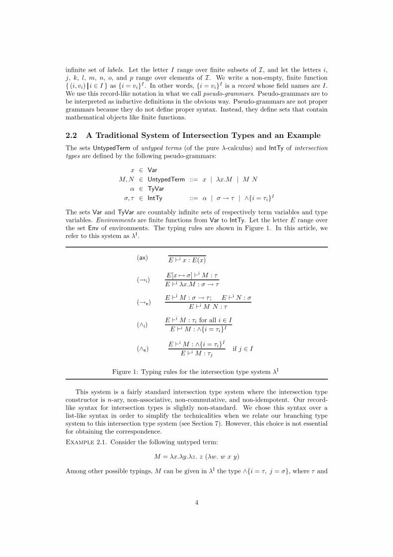
The sets Var and TyVar are countably infinite sets of respectively term variables and typevariables. Environments are finite functions from Var to IntTy. Let the letter E range overthe set Env of environments. The typing rules are shown in Figure 1. In this article, werefer to this system as λI.

(ax) E ì x : E(x)

(→i)E[x 7→ σ] ì M : τ

E ì λx.M : σ → τ

(→e)E ì M : σ → τ ; E ì N : σ

E ì M N : τ

(∧i)E ì M : τi for all i ∈ I

E ì M : ∧{i = τi}I

(∧e)E ì M : ∧{i = τi}

I

E ì M : τj

if j ∈ I

Figure 1: Typing rules for the intersection type system λI

This system is a fairly standard intersection type system where the intersection typeconstructor is n-ary, non-associative, non-commutative, and non-idempotent. Our record-like syntax for intersection types is slightly non-standard. We chose this syntax over alist-like syntax in order to simplify the technicalities when we relate our branching typesystem to this intersection type system (see Section 7). However, this choice is not essentialfor obtaining the correspondence.

Example 2.1. Consider the following untyped term:

M = λx.λy.λz. z (λw. w x y)

Among other possible typings, M can be given in λI the type ∧{i = τ, j = σ}, where τ and

4

σ are:

τ = (α → β) → α → τz → β

τz = (τw → β) → β

τw = (α → β) → α → β

σ = γ → ∧{m = γ → γ, n = β → β} → σz → β

σz = ∧{k = σwk → β, l = σw

l → β} → β

σwk = γ → (γ → γ) → β

σwl = γ → (β → β) → β

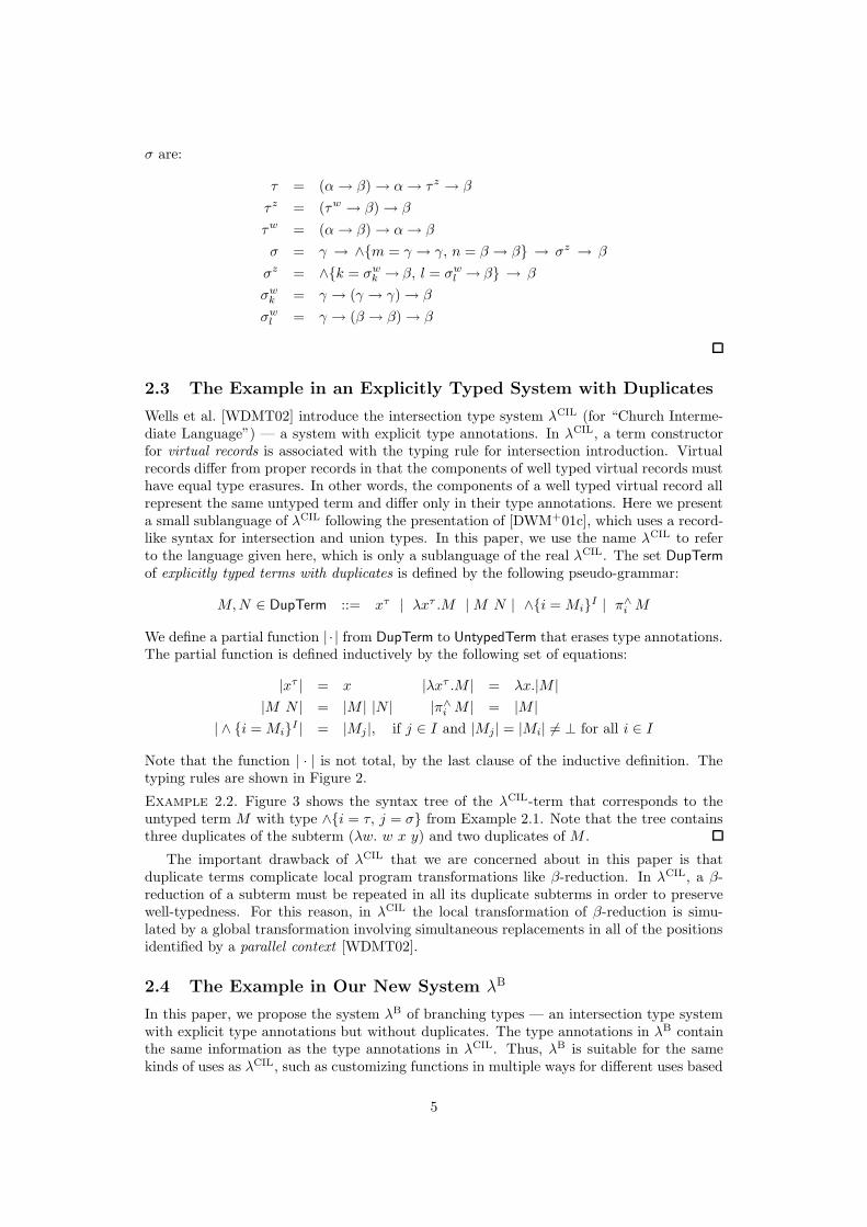
2.3 The Example in an Explicitly Typed System with Duplicates

Wells et al. [WDMT02] introduce the intersection type system λCIL (for “Church Interme-diate Language”) — a system with explicit type annotations. In λCIL, a term constructorfor virtual records is associated with the typing rule for intersection introduction. Virtualrecords differ from proper records in that the components of well typed virtual records musthave equal type erasures. In other words, the components of a well typed virtual record allrepresent the same untyped term and differ only in their type annotations. Here we presenta small sublanguage of λCIL following the presentation of [DWM+01c], which uses a record-like syntax for intersection and union types. In this paper, we use the name λCIL to referto the language given here, which is only a sublanguage of the real λCIL. The set DupTerm

of explicitly typed terms with duplicates is defined by the following pseudo-grammar:

M, N ∈ DupTerm ::= xτ | λxτ .M | M N | ∧{i = Mi}I | π∧

i M

We define a partial function | · | from DupTerm to UntypedTerm that erases type annotations.The partial function is defined inductively by the following set of equations:

|xτ | = x |λxτ .M | = λx.|M |

|M N | = |M | |N | |π∧i M | = |M |

| ∧ {i = Mi}I | = |Mj |, if j ∈ I and |Mj | = |Mi| 6= ⊥ for all i ∈ I

Note that the function | · | is not total, by the last clause of the inductive definition. Thetyping rules are shown in Figure 2.

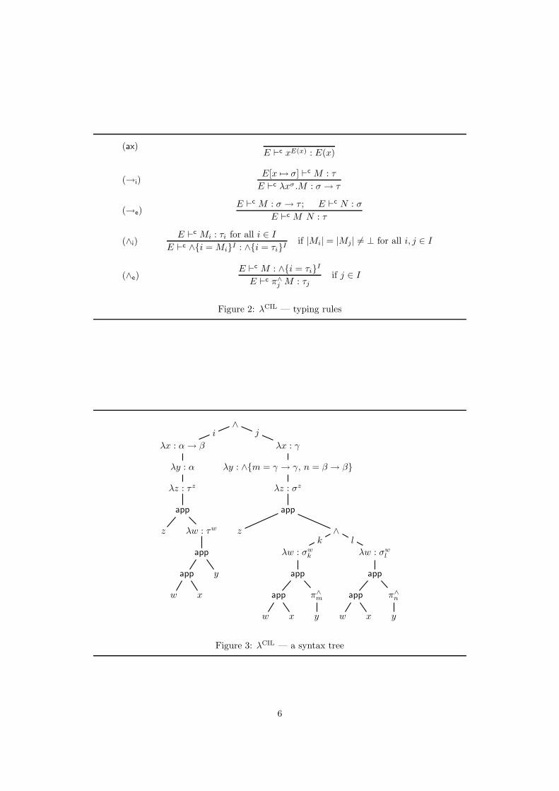
Example 2.2. Figure 3 shows the syntax tree of the λCIL-term that corresponds to theuntyped term M with type ∧{i = τ, j = σ} from Example 2.1. Note that the tree containsthree duplicates of the subterm (λw. w x y) and two duplicates of M .

The important drawback of λCIL that we are concerned about in this paper is thatduplicate terms complicate local program transformations like β-reduction. In λCIL, a β-reduction of a subterm must be repeated in all its duplicate subterms in order to preservewell-typedness. For this reason, in λCIL the local transformation of β-reduction is simu-lated by a global transformation involving simultaneous replacements in all of the positionsidentified by a parallel context [WDMT02].

2.4 The Example in Our New System λB

In this paper, we propose the system λB of branching types — an intersection type systemwith explicit type annotations but without duplicates. The type annotations in λB containthe same information as the type annotations in λCIL. Thus, λB is suitable for the samekinds of uses as λCIL, such as customizing functions in multiple ways for different uses based

5

(ax)E `c xE(x) : E(x)

(→i)E[x 7→ σ] `c M : τ

E `c λxσ .M : σ → τ

(→e)E `c M : σ → τ ; E `c N : σ

E `c M N : τ

(∧i)E `c Mi : τi for all i ∈ I

E `c ∧{i = Mi}I : ∧{i = τi}Iif |Mi| = |Mj | 6= ⊥ for all i, j ∈ I

(∧e)E `c M : ∧{i = τi}

I

E `c π∧j M : τj

if j ∈ I

Figure 2: λCIL — typing rules

∧

λx : α → β

i

λy : α

λz : τz

app

z λw : τw

app

app

w x

y

λx : γ

j

λy : ∧{m = γ → γ, n = β → β}

λz : σz

app

z ∧

λw : σwk

k

app

app

w x

π∧m

y

λw : σwl

l

app

app

w x

π∧n

y

Figure 3: λCIL — a syntax tree

6

Λ(join{i = ∗, j = ∗})

λx : {i = α → β, j = γ}

λy : {i = α, j = σyj }

λz : {i = τz , j = σzj }

app

z Λ{i = ∗, j = join{k = ∗, l = ∗}}

λw : {i = τw, j = {k = σwk , l = σw

l }}

app

app

w x

[{i = ∗, j = {k = (m, ∗), l = (n, ∗)}}]

y

Figure 4: λB — a syntax tree

on type annotations. On the other hand, β-reduction is simpler in λB and there is no needfor the use of parallel contexts in reduction.

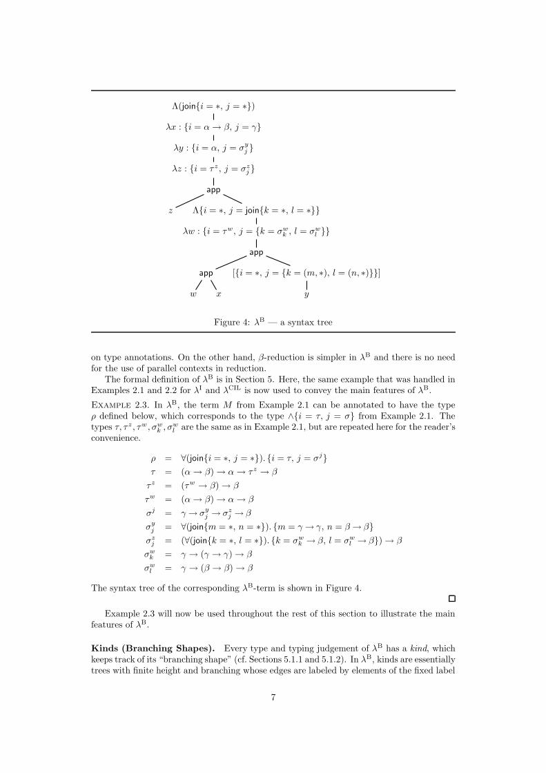
The formal definition of λB is in Section 5. Here, the same example that was handled inExamples 2.1 and 2.2 for λI and λCIL is now used to convey the main features of λB.

Example 2.3. In λB, the term M from Example 2.1 can be annotated to have the typeρ defined below, which corresponds to the type ∧{i = τ, j = σ} from Example 2.1. Thetypes τ, τz , τw , σw

k , σwl are the same as in Example 2.1, but are repeated here for the reader’s

convenience.

ρ = ∀(join{i = ∗, j = ∗}). {i = τ, j = σj}

τ = (α → β) → α → τz → β

τz = (τw → β) → β

τw = (α → β) → α → β

σj = γ → σyj → σz

j → β

σyj = ∀(join{m = ∗, n = ∗}). {m = γ → γ, n = β → β}

σzj = (∀(join{k = ∗, l = ∗}). {k = σw

k → β, l = σwl → β}) → β

σwk = γ → (γ → γ) → β

σwl = γ → (β → β) → β

The syntax tree of the corresponding λB-term is shown in Figure 4.

Example 2.3 will now be used throughout the rest of this section to illustrate the mainfeatures of λB.

Kinds (Branching Shapes). Every type and typing judgement of λB has a kind, whichkeeps track of its “branching shape” (cf. Sections 5.1.1 and 5.1.2). In λB, kinds are essentiallytrees with finite height and branching whose edges are labeled by elements of the fixed label

7

set I. These trees correspond in a certain way to the branching shapes of type derivationsin λI and, similarly, to the branching shapes of terms in λCIL.

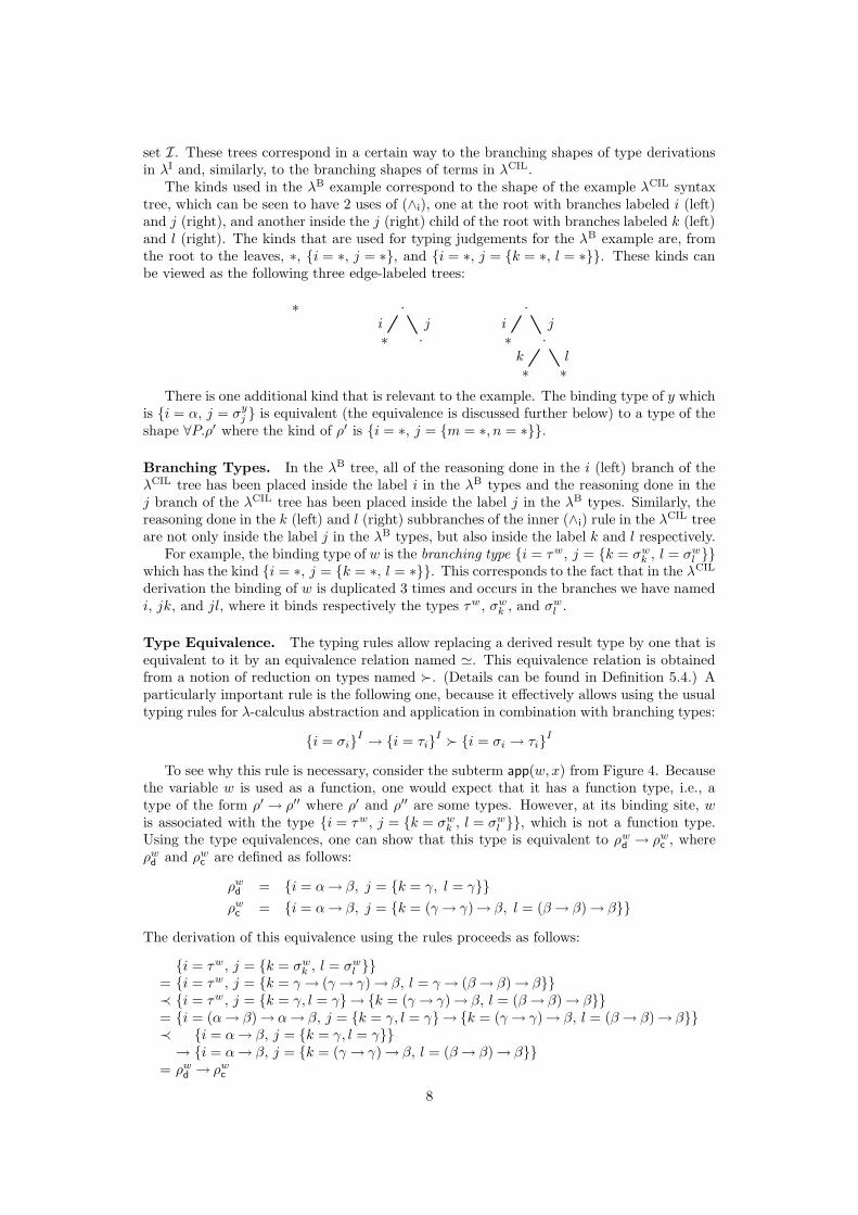
The kinds used in the λB example correspond to the shape of the example λCIL syntaxtree, which can be seen to have 2 uses of (∧i), one at the root with branches labeled i (left)and j (right), and another inside the j (right) child of the root with branches labeled k (left)and l (right). The kinds that are used for typing judgements for the λB example are, fromthe root to the leaves, ∗, {i = ∗, j = ∗}, and {i = ∗, j = {k = ∗, l = ∗}}. These kinds canbe viewed as the following three edge-labeled trees:

∗ ·

∗i

·j

·

∗i

·j

∗k

∗l

There is one additional kind that is relevant to the example. The binding type of y whichis {i = α, j = σ

yj } is equivalent (the equivalence is discussed further below) to a type of the

shape ∀P.ρ′ where the kind of ρ′ is {i = ∗, j = {m = ∗, n = ∗}}.

Branching Types. In the λB tree, all of the reasoning done in the i (left) branch of theλCIL tree has been placed inside the label i in the λB types and the reasoning done in thej branch of the λCIL tree has been placed inside the label j in the λB types. Similarly, thereasoning done in the k (left) and l (right) subbranches of the inner (∧i) rule in the λCIL treeare not only inside the label j in the λB types, but also inside the label k and l respectively.

For example, the binding type of w is the branching type {i = τw, j = {k = σwk , l = σw

l }}which has the kind {i = ∗, j = {k = ∗, l = ∗}}. This corresponds to the fact that in the λCIL

derivation the binding of w is duplicated 3 times and occurs in the branches we have namedi, jk, and jl, where it binds respectively the types τw , σw

k , and σwl .

Type Equivalence. The typing rules allow replacing a derived result type by one that isequivalent to it by an equivalence relation named '. This equivalence relation is obtainedfrom a notion of reduction on types named �. (Details can be found in Definition 5.4.) Aparticularly important rule is the following one, because it effectively allows using the usualtyping rules for λ-calculus abstraction and application in combination with branching types:

{i = σi}I→ {i = τi}

I� {i = σi → τi}

I

To see why this rule is necessary, consider the subterm app(w, x) from Figure 4. Becausethe variable w is used as a function, one would expect that it has a function type, i.e., atype of the form ρ′ → ρ′′ where ρ′ and ρ′′ are some types. However, at its binding site, w

is associated with the type {i = τw, j = {k = σwk , l = σw

l }}, which is not a function type.Using the type equivalences, one can show that this type is equivalent to ρw

d → ρwc , where

ρwd and ρw

c are defined as follows:

ρwd = {i = α → β, j = {k = γ, l = γ}}

ρwc = {i = α → β, j = {k = (γ → γ) → β, l = (β → β) → β}}

The derivation of this equivalence using the rules proceeds as follows:

{i = τw , j = {k = σwk , l = σw

l }}= {i = τw , j = {k = γ → (γ → γ) → β, l = γ → (β → β) → β}}≺ {i = τw , j = {k = γ, l = γ}→ {k = (γ → γ) → β, l = (β → β) → β}}= {i = (α → β) → α → β, j = {k = γ, l = γ}→ {k = (γ → γ) → β, l = (β → β) → β}}≺ {i = α → β, j = {k = γ, l = γ}}

→ {i = α → β, j = {k = (γ → γ) → β, l = (β → β) → β}}= ρw

d → ρwc

8

Hence, although w’s type is not equal to a function type, it is equal to a function typemodulo our notion of type equivalence.

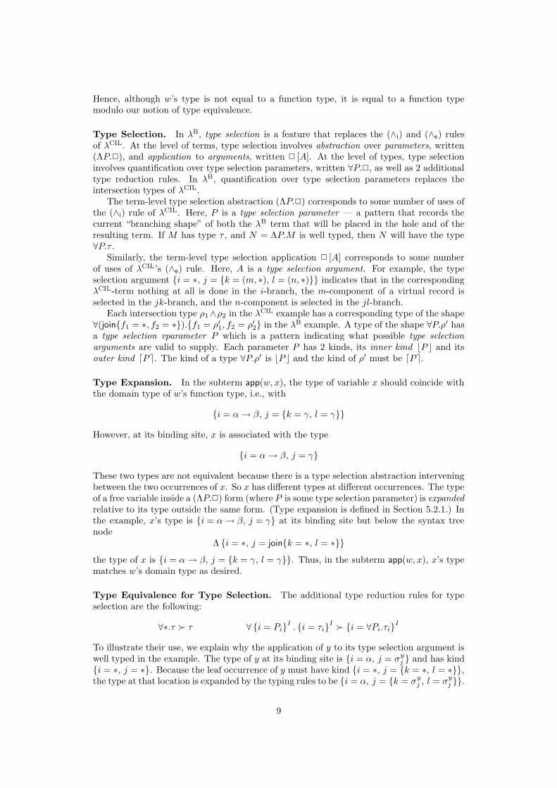
Type Selection. In λB, type selection is a feature that replaces the (∧i) and (∧e) rulesof λCIL. At the level of terms, type selection involves abstraction over parameters, written(ΛP.2), and application to arguments, written 2 [A]. At the level of types, type selectioninvolves quantification over type selection parameters, written ∀P.2, as well as 2 additionaltype reduction rules. In λB, quantification over type selection parameters replaces theintersection types of λCIL.

The term-level type selection abstraction (ΛP.2) corresponds to some number of uses ofthe (∧i) rule of λCIL. Here, P is a type selection parameter — a pattern that records thecurrent “branching shape” of both the λB term that will be placed in the hole and of theresulting term. If M has type τ , and N = ΛP.M is well typed, then N will have the type∀P.τ .

Similarly, the term-level type selection application 2 [A] corresponds to some numberof uses of λCIL’s (∧e) rule. Here, A is a type selection argument. For example, the typeselection argument {i = ∗, j = {k = (m, ∗), l = (n, ∗)}} indicates that in the correspondingλCIL-term nothing at all is done in the i-branch, the m-component of a virtual record isselected in the jk-branch, and the n-component is selected in the jl-branch.

Each intersection type ρ1∧ρ2 in the λCIL example has a corresponding type of the shape∀(join{f1 = ∗, f2 = ∗}).{f1 = ρ′1, f2 = ρ′2} in the λB example. A type of the shape ∀P.ρ′ hasa type selection vparameter P which is a pattern indicating what possible type selectionarguments are valid to supply. Each parameter P has 2 kinds, its inner kind bP c and itsouter kind dP e. The kind of a type ∀P.ρ′ is bP c and the kind of ρ′ must be dP e.

Type Expansion. In the subterm app(w, x), the type of variable x should coincide withthe domain type of w’s function type, i.e., with

{i = α → β, j = {k = γ, l = γ}}

However, at its binding site, x is associated with the type

{i = α → β, j = γ}

These two types are not equivalent because there is a type selection abstraction interveningbetween the two occurrences of x. So x has different types at different occurrences. The typeof a free variable inside a (ΛP.2) form (where P is some type selection parameter) is expandedrelative to its type outside the same form. (Type expansion is defined in Section 5.2.1.) Inthe example, x’s type is {i = α → β, j = γ} at its binding site but below the syntax treenode

Λ {i = ∗, j = join{k = ∗, l = ∗}}

the type of x is {i = α → β, j = {k = γ, l = γ}}. Thus, in the subterm app(w, x), x’s typematches w’s domain type as desired.

Type Equivalence for Type Selection. The additional type reduction rules for typeselection are the following:

∀∗.τ � τ ∀ {i = Pi}I. {i = τi}

I� {i = ∀Pi.τi}

I

To illustrate their use, we explain why the application of y to its type selection argument iswell typed in the example. The type of y at its binding site is {i = α, j = σ

yj } and has kind

{i = ∗, j = ∗}. Because the leaf occurrence of y must have kind {i = ∗, j = {k = ∗, l = ∗}},the type at that location is expanded by the typing rules to be {i = α, j = {k = σ

yj , l = σ

yj }}.

9

For the sake of the example, we now use some additional names to abbreviate portions ofthe types:

Pmn = join{m = ∗, n = ∗}σ

yj2 = {m = γ → γ, n = β → β}

Thus, σyj = ∀Pmn.σ

yj2. Type equivalences can now be applied to the type as follows to lift

the occurrences of ∀P to outermost position:

{i = α, j = {k = σyj , l = σ

yj }}

' {i = (∀∗.α), j = ∀{k = Pmn, l = Pmn}.{k = σyj2, l = σ

yj2}}

' ∀{i = ∗, j = {k = Pmn, l = Pmn}}.{i = α, j = {k = σyj2, l = σ

yj2}}

The final type is the type actually used in figure 4. The type selection parameter of the finaltype is {i = ∗, j = {k = Pmn, l = Pmn}} which effectively says, “in the i branch, no typeselection argument can be supplied and in the jk and jl branches, a choice between m andn can be supplied”. The type selection argument {i = ∗, j = {k = (m, ∗), l = (n, ∗)}} in factdoes just this; it supplies no choice in the i branch, a choice of m in the jk branch, and achoice of n in the jl branch. The ∗ in (m, ∗) means that after the choice of m is supplied,no further choices are supplied.

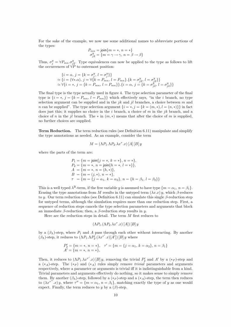
Term Reduction. The term reduction rules (see Definition 6.11) manipulate and simplifythe type annotations as needed. As an example, consider the term

M = (ΛP1.ΛP2.λxτ .x) [A] [B] y

where the parts of the term are:

P1 = {m = join{j = ∗, k = ∗}, n = ∗},P2 = {m = ∗, n = join{h = ∗, l = ∗}},A = {m = ∗, n = (h, ∗)},B = {m = (j, ∗), n = ∗},τ = {m = {j = α1, k = α2}, n = {h = β1, l = β2}}

This is a well typed λB-term, if the free variable y is assumed to have type {m = α1, n = β1}.Erasing the type annotations from M results in the untyped term (λx.x) y, which β-reducesto y. Our term reduction rules (see Definition 6.11) can simulate this single β-reduction stepfor untyped terms, although the simulation requires more than one reduction step. First, asequence of reduction steps cancels the type selection parameters and arguments that blockan immediate β-reduction; then, a β-reduction step results in y.

Here are the reduction steps in detail. The term M first reduces to

(ΛP1.(ΛP2.λxτ .x) [A]) [B] y

by a (βΛ)-step, where P1 and A pass through each other without interacting. By another(βΛ)-step, it reduces to (ΛP1.ΛP ′

2.(λxτ ′

.x)[A′]) [B] y where

P ′2 = {m = ∗, n = ∗},

A′ = {m = ∗, n = ∗},τ ′ = {m = {j = α1, k = α2}, n = β1}

Then, it reduces to (ΛP1.λxτ ′

.x) [B] y, removing the trivial P ′2 and A′ by a (∗P )-step and

a (∗A)-step. The (∗P ) and (∗A) rules simply remove trivial parameters and argumentsrespectively, where a parameter or arguments is trivial iff it is indistinguishable from a kind.Trivial parameters and arguments effectively do nothing, so it makes sense to simply removethem. By another (βΛ)-step, followed by a (∗P )-step and a (∗A)-step, the term then reducesto (λxτ ′′

.x) y, where τ ′′ = {m = α1, n = β1}, matching exactly the type of y as one wouldexpect. Finally, the term reduces to y by a (β)-step.

10

3 Comparison to Recent Related Work

Ronchi Della Rocca and Roversi have a system called Intersection Logic (IL) [RDRR01]which is similar to λB, but has nothing corresponding to our explicitly typed terms. ILhas a meta-level operation corresponding to our equivalence for function types. IL hasnothing corresponding to our other type equivalences, because IL does not group paralleloccurrences of its equivalent of type selection parameters and arguments, but instead workswith equivalence classes of derivations modulo permutations of what we call individual typeselection parameters and arguments. We expect that the use of these equivalence classeswill cause great difficulty with the proofs for IL. Much of the proof burden for the IL system(corresponding to a large portion of this paper) is inside the 3-word proof (“by structuralinduction”) of their lemma 4 in the calculation of S(Π, Π′) where S is not constructivelyspecified. A proof-term-labeled version of IL is presented, but the proof terms are pureλ-terms and thus the proof terms do not represent entire derivations.

Capitani, Loreti, and Venneri have designed a similar system called HL (HyperformulaeLogic) [CLV01]. HL is quite similar to IL, although it seems overall to have a less complicatedpresentation. HL has nothing corresponding to our equivalences on types. The set ofproperties proved for HL in [CLV01] is not exactly the same as the set of properties provedfor IL in [RDRR01], e.g., there is no attempt to directly prove any result related to reductionof HL proofs as there is for IL, although this could be obtained indirectly via their proofs ofequivalence with traditional systems with intersection types. HL is reported in [RDRR01]to have a typed version of an untyped calculus like that in [Kfo00], but in fact there is nosignificant connection between [CLV01] and [Kfo00] and there is no explicitly typed calculusassociated with HL.1

As for λB, for both IL and HL there are proofs of equivalence with more traditionalsystems with intersection types. These proofs show that the proof-term-annotated versionsof IL and HL can type the same sets of pure untyped λ-terms as a traditional system withintersection types. The correspondence we show for λB involves a notion of type erasurewhile the correspondences for IL and HL do not as their proof terms are pure non-type-annotated λ-terms.

4 Conclusion

In this paper, we present λB, the first explicitly typed calculus with the power of intersectiontypes which is Church-style, i.e., typed terms contain explicit type annotations and donot have multiple disjoint subterms corresponding to single subterms in the correspondinguntyped term. Branching types are used in λB to represent the effect of what is handledwith simultaneous derivations in systems with intersection types. We prove for λB subjectreduction, and soundness and completeness of explicitly typed reduction w.r.t. β-reductionon the corresponding untyped λ-terms. Moreover, we formally relate λB to a traditionalintersection type system where terms do not have explicit type annotations. The mainbenefit of λB will be to make it easier to use technology (both theories and software) alreadydeveloped for the λ-calculus on explicitly typed terms in a type system having the powerand flexibility of intersection types. Due to the experimental performance measurementsreported in [DWM+01b], we do not expect a substantial size benefit in practice from λB

over λCIL. In the area of logic, λB terms may be useful as explicitly typed realizers ofthe so-called strong conjunction, but we are not currently planning on investigating thisourselves.

1It seems there may have been one in an unpublished version of the paper.

11

Part II

Technical Presentation

This part presents formal definitions, lemmas, and theorems as well as a number of examples.The reader interested in the motivations and implications of our new system λB will findthem in part I.

4.1 Partial Functions

In this paragraph, we fix some definitions and notational conventions concerning partialfunctions: If X is a set not containing an element by the name ⊥, then X⊥ denotes thepartially ordered set (X⊥,≤), where

X⊥ =def== X ∪ {⊥} ; (x ≤ y) ⇐

def=⇒ (x = ⊥)

A function from X⊥ to Y⊥ is called strict if it maps ⊥ to ⊥. In this article, partial functionsfrom a set X to a set Y are defined as strict, total functions from X⊥ to Y⊥. Suppose that f isa partial function from X to Y , x ∈ X and y ∈ Y . We say that f(x) is undefined if f(x) = ⊥.Otherwise, we say that f(x) is defined. The domain of f is the set {x f(x) is defined } and isdenoted by dom(f). The range of f is the set { f(x) x ∈ dom(f) } and is denoted by ran(f).The expression f [x 7→ y] denotes the partial function { (x′, y) ∈ f x′ 6= x } ∪ {(x, y)}. Afinite function from X to Y is a partial function from X to Y that has a finite domain.

Partial functions are ordered pointwise. That is, if f, g are partial functions from X toY , then (f ≤ g) iff (f(x) ≤ g(x)) for all x ∈ X . We will often define partial functionsinductively by sets of equations. Such inductive definitions define the least partial function(with respect to the pointwise ordering) that satisfies the given equations. For all setsX1, . . . , Xn, the function smash is defined as follows:

smash : X1 × · · · × Xn → (X1 × · · · × Xn)⊥

smash(x1, . . . , xn) =

{

⊥ if xi = ⊥ for some i in {1 . . . n}(x1, . . . , xn) otherwise

In expressions that involve partial functions, we usually omit smashes and let the contextresolve ambiguities. For example, if f is a partial function from X × X × X to X , g isa partial function from X to X , and x, y, z are elements of X , then f(g(x), g(y), z) is anabbreviation for f(smash(g(x), g(y), z)).

Given a binary relation R on a set X , we lift it to a binary relation R⊥ on X⊥ as follows:

(x1 R⊥ x2) ⇐def=⇒ (x1 = x2 = ⊥) or (x1 R x2)

We will make use of the following facts:

• If R is an equivalence relation on X , then R⊥ is an equivalence relation on X⊥.

• If R is an equivalence relation on X , (x R⊥ y), and (y R z), then (x R z). (Theomissions of the superscripts are intentional.)

5 The Branching Type System λB

5.1 Types and Kinds

5.1.1 Kinds

The set Kind of kinds is defined by the following pseudo-grammar:

κ ∈ Kind ::= ∗ | {i = κi}I

12

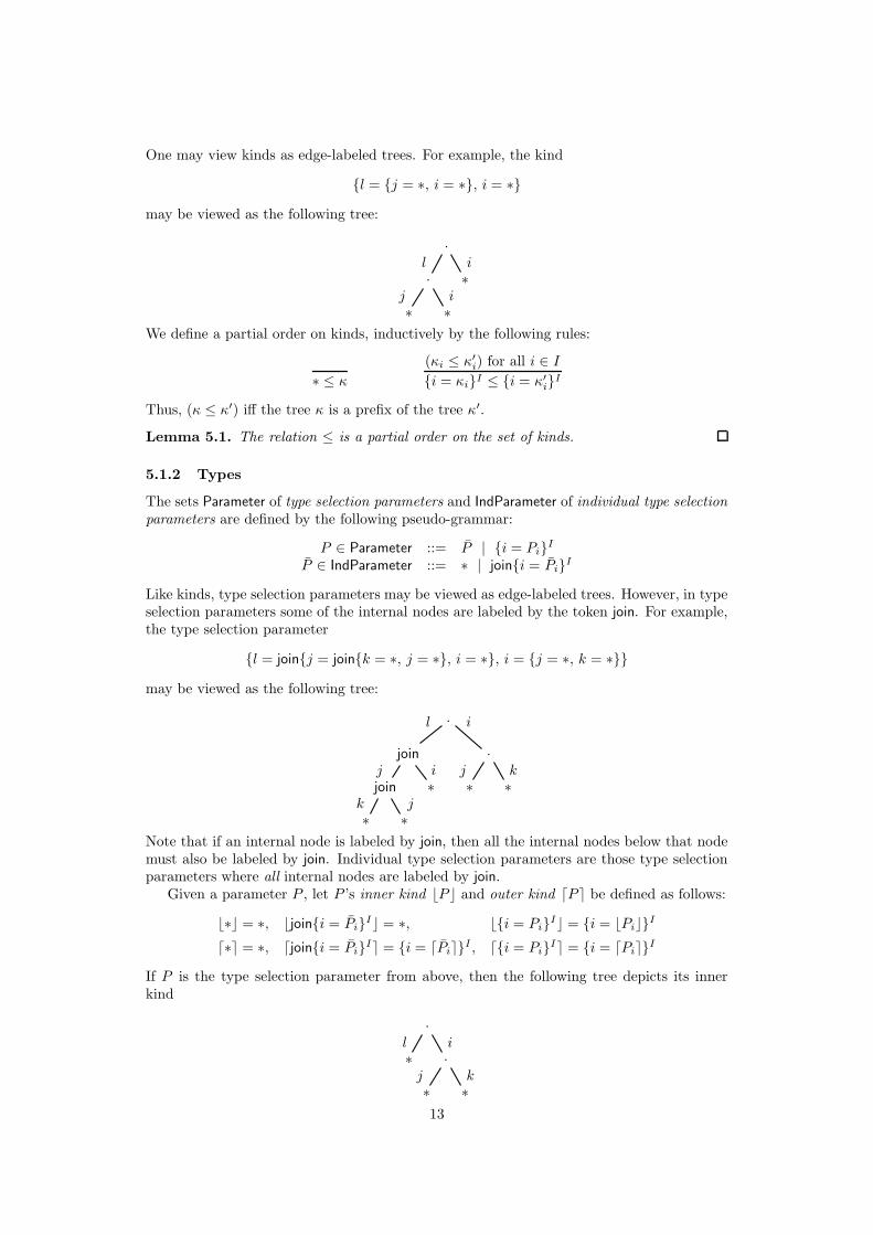
One may view kinds as edge-labeled trees. For example, the kind

{l = {j = ∗, i = ∗}, i = ∗}

may be viewed as the following tree:

·

·l

∗j

∗i∗i

We define a partial order on kinds, inductively by the following rules:

∗ ≤ κ

(κi ≤ κ′i) for all i ∈ I

{i = κi}I ≤ {i = κ′i}

I

Thus, (κ ≤ κ′) iff the tree κ is a prefix of the tree κ′.

Lemma 5.1. The relation ≤ is a partial order on the set of kinds.

5.1.2 Types

The sets Parameter of type selection parameters and IndParameter of individual type selectionparameters are defined by the following pseudo-grammar:

P ∈ Parameter ::= P | {i = Pi}I

P ∈ IndParameter ::= ∗ | join{i = Pi}I

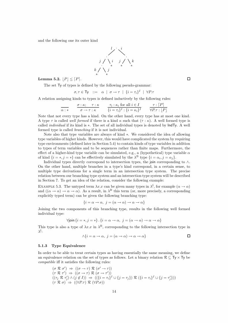
Like kinds, type selection parameters may be viewed as edge-labeled trees. However, in typeselection parameters some of the internal nodes are labeled by the token join. For example,the type selection parameter

{l = join{j = join{k = ∗, j = ∗}, i = ∗}, i = {j = ∗, k = ∗}}

may be viewed as the following tree:

·

join

l

joinj

∗k

∗j

∗i

·

i

∗j

∗k

Note that if an internal node is labeled by join, then all the internal nodes below that nodemust also be labeled by join. Individual type selection parameters are those type selectionparameters where all internal nodes are labeled by join.

Given a parameter P , let P ’s inner kind bP c and outer kind dP e be defined as follows:

b∗c = ∗, bjoin{i = Pi}Ic = ∗, b{i = Pi}

Ic = {i = bPic}I

d∗e = ∗, djoin{i = Pi}Ie = {i = dPie}

I , d{i = Pi}Ie = {i = dPie}

I

If P is the type selection parameter from above, then the following tree depicts its innerkind

·

∗l

·i

∗j

∗k

13

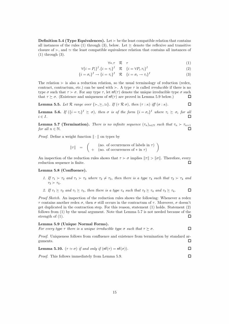
and the following one its outer kind

·

·

l

·j

∗k

∗j∗i

·

i

∗j

∗k

Lemma 5.2. bP c ≤ dP e.

The set Ty of types is defined by the following pseudo-grammar:

σ, τ ∈ Ty ::= α | σ → τ | {i = τi}I | ∀P.τ

A relation assigning kinds to types is defined inductively by the following rules:

α : ∗

σ : κ; τ : κ

σ → τ : κ

τi : κi for all i ∈ I

{i = τi}I : {i = κi}I

τ : dP e

∀P.τ : bP c

Note that not every type has a kind. On the other hand, every type has at most one kind.A type τ is called well formed if there is a kind κ such that (τ : κ). A well formed type iscalled individual if its kind is ∗. The set of all individual types is denoted by IndTy. A wellformed type is called branching if it is not individual.

Note also that type variables are always of kind ∗. We considered the idea of allowingtype variables of higher kinds. However, this would have complicated the system by requiringtype environments (defined later in Section 5.4) to contain kinds of type variables in additionto types of term variables and to be sequences rather than finite maps. Furthermore, theeffect of a higher-kind type variable can be simulated, e.g., a (hypothetical) type variable α

of kind {i = ∗, j = ∗} can be effectively simulated by the λB type {i = αi, j = αj}.Individual types directly correspond to intersection types, the join corresponding to ∧.

On the other hand, multiple branches in a type’s kind correspond, in a certain sense, tomultiple type derivations for a single term in an intersection type system. The preciserelation between our branching type system and an intersection type system will be describedin Section 7. To get an idea of the relation, consider the following example:

Example 5.3. The untyped term λx.x can be given many types in λI, for example (α → α)and ((α → α) → α → α). As a result, in λB this term (or, more precisely, a correspondingexplicitly typed term) can be given the following branching type:

{i = α → α, j = (α → α) → α → α}

Joining the two components of this branching type, results in the following well formedindividual type:

∀join {i = ∗, j = ∗} . {i = α → α, j = (α → α) → α → α}

This type is also a type of λx.x in λB, corresponding to the following intersection type inλI:

∧{i = α → α, j = (α → α) → α → α}

5.1.3 Type Equivalence

In order to be able to treat certain types as having essentially the same meaning, we definean equivalence relation on the set of types as follows. Let a binary relation R ⊆ Ty ×Ty becompatible iff it satisfies the following rules:

(σ R σ′) ⇒ ((σ → τ) R (σ′ → τ))(τ R τ ′) ⇒ ((σ → τ) R (σ → τ ′))((τj R τ ′

j) ∧ (j 6∈ I)) ⇒ (({i = τi}I ∪ {j = τj}) R ({i = τi}

I ∪ {j = τ ′j}))

(τ R σ) ⇒ ((∀P.τ) R (∀P.σ))

14

Definition 5.4 (Type Equivalences). Let � be the least compatible relation that containsall instances of the rules (1) through (3), below. Let � denote the reflexive and transitiveclosure of �, and ' the least compatible equivalence relation that contains all instances of(1) through (3).

∀∗.τ R τ (1)

∀{i = Pi}I .{i = τi}

I R {i = ∀Pi.τi}I (2)

{i = σi}I → {i = τi}

I R {i = σi → τi}I (3)

The relation � is also a reduction relation, so the usual terminology of reduction (redex,contract, contractum, etc.) can be used with �. A type τ is called irreducible if there is notype σ such that τ � σ. For any type τ , let nf(τ) denote the unique irreducible type σ suchthat τ � σ. (Existence and uniqueness of nf(τ) are proved in Lemma 5.9 below.)

Lemma 5.5. Let R range over {�,�,'}. If (τ R σ), then (τ : κ) iff (σ : κ).

Lemma 5.6. If ({i = τi}I � σ), then σ is of the form {i = σi}

I where τi � σi for alli ∈ I.

Lemma 5.7 (Termination). There is no infinite sequence (τn)n∈N such that τn � τn+1

for all n ∈ N.

Proof. Define a weight function ‖ · ‖ on types by

‖τ‖ =

(

(no. of occurrences of labels in τ)+ (no. of occurrences of ∗ in τ)

)

An inspection of the reduction rules shows that τ � σ implies ‖τ‖ > ‖σ‖. Therefore, everyreduction sequence is finite.

Lemma 5.8 (Confluence).

1. If τ1 � τ2 and τ1 � τ3 where τ2 6= τ3, then there is a type τ4 such that τ2 � τ4 andτ3 � τ4.

2. If τ1 � τ2 and τ1 � τ3, then there is a type τ4 such that τ2 � τ4 and τ3 � τ4.

Proof Sketch. An inspection of the reduction rules shows the following: Whenever a redexτ contains another redex σ, then σ still occurs in the contractum of τ . Moreover, σ doesn’tget duplicated in the contraction step. For this reason, statement (1) holds. Statement (2)follows from (1) by the usual argument. Note that Lemma 5.7 is not needed because of thestrength of (1).

Lemma 5.9 (Unique Normal Forms).For every type τ there is a unique irreducible type σ such that τ � σ.

Proof. Uniqueness follows from confluence and existence from termination by standard ar-guments.

Lemma 5.10. (τ ' σ) if and only if (nf(τ) = nf(σ)).

Proof. This follows immediately from Lemma 5.9.

15

5.1.4 A Grammar for Normal Types

An important property of irreducible types is that their top-level structure reflects the top-level structure of their kinds. In particular, if a type is irreducible and individual, then itis not of the form {i = τi}

I . The following grammatical characterization helps make thisprecise.

Let P • range over (IndParameter−{∗}) (i.e., over individual type selection parameters ofthe form join{i = Pi}

I). The sets NormalTy of normal types and IndNormalTy of individualnormal types are defined by the following pseudo-grammars:

µ, ν ∈ NormalTy ::= µ | {i = µi}I

µ, ν ∈ IndNormalTy ::= α | µ → ν | ∀P •.µ

Let normal(τ) abbreviate the statement that τ is normal. By Lemma 5.12 below, normalityand irreducibility are equivalent for well formed types.

Lemma 5.11. If (τ : {i = κi}I) and τ is irreducible, then τ is of the form {i = τi}

I whereτi : κi for all i ∈ I.

Proof. By induction on the derivation of (τ : {i = κi}I).

Lemma 5.12.

1. If (µ ∈ NormalTy), then (µ ∈ Ty).

2. If (µ ∈ IndNormalTy) and µ is well formed (i.e., µ : κ for some κ), then (µ ∈ IndTy)(i.e., κ = ∗).

3. If (τ ∈ IndTy) (i.e., τ : ∗) and (τ ∈ NormalTy), then (τ ∈ IndNormalTy).

4. If µ is normal, then µ is irreducible.

5. If τ is well formed and irreducible, then τ is normal.

5.1.5 Type Matching

For type checking in λB, it is necessary to have an algorithm that decides whether a giventype σ matches a function type, i.e., whether there are types τ, τ ′ such that (σ ' τ → τ ′).Lemma 5.14(2) gives a simple decision algorithm for this question. Lemma 5.13(2) says thatall possible ways of matching a function type are equivalent. In addition to function types,we also establish similar statements for branching types and ∀-types. The results of thissection can easily be combined to make a general matching algorithm for ', although we donot do so because we do not need such an algorithm in this paper.

Lemma 5.13.

1. If ({i = τi}I ' {i = σi}

I), then (τi ' σi) for all i ∈ I.

2. If (τ → τ ′ ' σ → σ′), then (τ ' τ ′) and (σ ' σ′).

3. If (∀P.τ ' ∀P.τ ′), then (τ ' τ ′).

Proof. Statement (1) follows from Lemmas 5.10 and 5.6. Statement (2) is proved by induc-tion on the size of (τ → τ ′)’s �-reduction graph. Statement (3) is proved by induction onthe size of (∀P.τ)’s �-reduction graph.

16

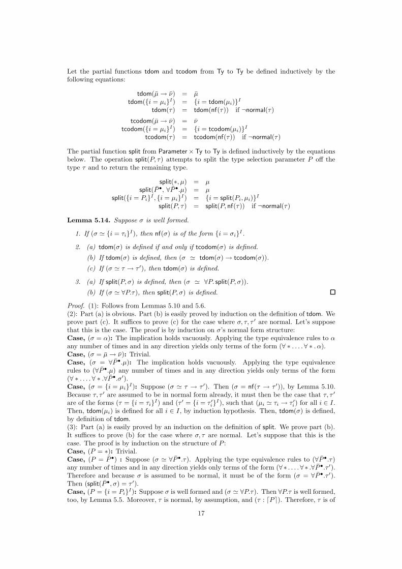
Let the partial functions tdom and tcodom from Ty to Ty be defined inductively by thefollowing equations:

tdom(µ → ν) = µ

tdom({i = µi}I) = {i = tdom(µi)}

I

tdom(τ) = tdom(nf(τ)) if ¬normal(τ)

tcodom(µ → ν) = ν

tcodom({i = µi}I) = {i = tcodom(µi)}

I

tcodom(τ) = tcodom(nf(τ)) if ¬normal(τ)

The partial function split from Parameter ×Ty to Ty is defined inductively by the equationsbelow. The operation split(P, τ) attempts to split the type selection parameter P off thetype τ and to return the remaining type.

split(∗, µ) = µ

split(P •, ∀P •.µ) = µ

split({i = Pi}I , {i = µi}

I) = {i = split(Pi, µi)}I

split(P, τ) = split(P, nf(τ)) if ¬normal(τ)

Lemma 5.14. Suppose σ is well formed.

1. If (σ ' {i = τi}I), then nf(σ) is of the form {i = σi}

I .

2. (a) tdom(σ) is defined if and only if tcodom(σ) is defined.

(b) If tdom(σ) is defined, then (σ ' tdom(σ) → tcodom(σ)).

(c) If (σ ' τ → τ ′), then tdom(σ) is defined.

3. (a) If split(P, σ) is defined, then (σ ' ∀P. split(P, σ)).

(b) If (σ ' ∀P.τ), then split(P, σ) is defined.

Proof. (1): Follows from Lemmas 5.10 and 5.6.(2): Part (a) is obvious. Part (b) is easily proved by induction on the definition of tdom. Weprove part (c). It suffices to prove (c) for the case where σ, τ, τ ′ are normal. Let’s supposethat this is the case. The proof is by induction on σ’s normal form structure:Case, (σ = α): The implication holds vacuously. Applying the type equivalence rules to α

any number of times and in any direction yields only terms of the form (∀ ∗ . . . . ∀ ∗ . α).Case, (σ = µ → ν): Trivial.Case, (σ = ∀P •.µ): The implication holds vacuously. Applying the type equivalencerules to (∀P •.µ) any number of times and in any direction yields only terms of the form(∀ ∗ . . . .∀ ∗ .∀P •.σ′).Case, (σ = {i = µi}

I): Suppose (σ ' τ → τ ′). Then (σ = nf(τ → τ ′)), by Lemma 5.10.Because τ, τ ′ are assumed to be in normal form already, it must then be the case that τ, τ ′

are of the forms (τ = {i = τi}I) and (τ ′ = {i = τ ′

i}I), such that (µi ' τi → τ ′

i ) for all i ∈ I .Then, tdom(µi) is defined for all i ∈ I , by induction hypothesis. Then, tdom(σ) is defined,by definition of tdom.(3): Part (a) is easily proved by an induction on the definition of split. We prove part (b).It suffices to prove (b) for the case where σ, τ are normal. Let’s suppose that this is thecase. The proof is by induction on the structure of P :Case, (P = ∗): Trivial.Case, (P = P •) : Suppose (σ ' ∀P •.τ). Applying the type equivalence rules to (∀P •.τ)any number of times and in any direction yields only terms of the form (∀∗ . . . .∀∗ .∀P •.τ ′).Therefore and because σ is assumed to be normal, it must be of the form (σ = ∀P •.τ ′).Then (split(P •, σ) = τ ′).Case, (P = {i = Pi}

I): Suppose σ is well formed and (σ ' ∀P.τ). Then ∀P.τ is well formed,too, by Lemma 5.5. Moreover, τ is normal, by assumption, and (τ : dP e). Therefore, τ is of

17

the form {i = τi}I . By Lemma 5.5, it is the case that (σ : bP c). Then, because σ is assumed

normal, it is the case that σ is of the form {i = µi}I . Because (σ ' ∀P.τ ' {i = ∀Pi.τi}

I),it is the case that (µi ' ∀Pi.τi) for all i ∈ I , by Lemma 5.13(1). Then, split(Pi, µi) is definedfor all i ∈ I , by induction hypothesis. Then, split(P, σ) is defined, by definition of split.

5.2 Expansion and Selection for Types

5.2.1 Type Expansion

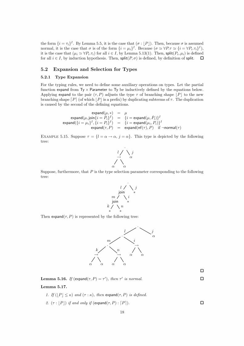
For the typing rules, we need to define some auxiliary operations on types. Let the partialfunction expand from Ty × Parameter to Ty be inductively defined by the equations below.Applying expand to the pair (τ, P ) adjusts the type τ of branching shape bP c to the newbranching shape dP e (of which bP c is a prefix) by duplicating subterms of τ . The duplicationis caused by the second of the defining equations.

expand(µ, ∗) = µ

expand(µ, join{i = Pi}I) = {i = expand(µ, Pi)}

I

expand({i = µi}I , {i = Pi}

I) = {i = expand(µi, Pi)}I

expand(τ, P ) = expand(nf(τ), P ) if ¬normal(τ)

Example 5.15. Suppose τ = {l = α → α, j = α}. This type is depicted by the followingtree:

·

→l

α α

αj

Suppose, furthermore, that P is the type selection parameter corresponding to the followingtree:

·

joinl

joinm

∗k

∗n

∗i

∗j

Then expand(τ, P ) is represented by the following tree:

·

·l

·m

→k

α α

→n

α α

→i

α α

αj

Lemma 5.16. If (expand(τ, P ) = τ ′), then τ ′ is normal.

Lemma 5.17.

1. If (bP c ≤ κ) and (τ : κ), then expand(τ, P ) is defined.

2. (τ : bP c) if and only if (expand(τ, P ) : dP e).

18

Proof. To prove part (1), one first proves the statement for the case where τ is normal, byinduction on the structure of P and using Lemma 5.11. Then, for the case where τ is notnormal, one uses the fact that normalization preserves kinds (Lemma 5.5). The proof ofpart (2) follows the same strategy.

Lemma 5.18. If (expand(τ, P ) ' expand(τ ′, P )), then (τ ' τ ′).

Proof. It suffices to prove the statement for the case where τ and τ ′ are normal. For thiscase, it is proved by induction on the structure of P .

Lemma 5.19.

1. If expand({i = τi}I , P ) is defined, then P is of the form {i = P ′

i}I .

2. expand({i = τi}I , {i = Pi}

I) '⊥ {i = expand(τi, Pi)}I .

3. expand(σ → τ, P ) '⊥ expand(σ, P ) → expand(τ, P ).

Proof. Parts (1) and (2) are obvious for normal types. For non-normal types, they followfrom Lemma 5.6. For normal types, part (3) is proved by induction on the structure of P .For non-normal types, part (3) is proved by induction on the size of the �-reduction-graphof (σ → τ), using parts (1) and (2).

5.2.2 Type Selection Arguments and Selection for Types

The sets Argument of type selection arguments and IndArgument of individual type selectionarguments are defined by the following pseudo-grammar:

A ∈ Argument ::= A | {i = Ai}I

A ∈ IndArgument ::= ∗ | i, A

We define two relations that assign kinds to arguments:

∗ : ∗

A : ∗

i, A : ∗

Ai : κi for all i ∈ I

{i = Ai}I : {i = κi}I

∗ / κ

A / κj

j, A / {i = κi}Iif j ∈ I

Ai / κi for all i ∈ I

{i = Ai}I / {i = κi}I

Note that for every argument A there is exactly one kind κ such that (A : κ). On the otherhand, there are many kinds κ such that (A / κ).

Lemma 5.20. If (A / κ) and (κ ≤ κ′), then (A / κ′).

We define two partial functions selecti and selectb, both from Ty × Argument to Ty,inductively by the equations below. The two functions are similar. The main differenceis that selecti performs selections on individual (joined) types, whereas selectb performsselections on branching types. Another difference is that selectb(µ, ∗) is always defined,whereas selecti(µ, ∗) is only defined if µ is an individual type.

selecti(µ, ∗) = µ

selecti(∀(join{i = Pi}I).{i = µi}

I , (j, A)) = selecti(∀Pj .µj , A), if (j ∈ I)

selecti({i = µi}I , {i = Ai}

I) = {i = selecti(µi, Ai)}I

selecti(τ, A) = select

i(nf(τ), A) if ¬normal(τ)

selectb(µ, ∗) = µ

selectb({i = µi}I , (j, A)) = selectb(µj , A), if (j ∈ I)

selectb({i = µi}I , {i = Ai}

I) = {i = selectb(µi, Ai)}I

selectb(τ, A) = selectb(nf(τ), A) if ¬normal(τ)

19

Lemma 5.21. If f ∈ {selecti, selectb} and f(τ, A) = τ ′, then τ ′ is normal.

Lemma 5.22.

1. If (τ : κ) and selecti(τ, A) is defined, then (A : κ).

2. If (τ : κ) and (selecti(τ, A) = τ ′), then (τ ′ : κ).

3. If (τ : κ), then (A / κ) if and only if selectb(τ, A) is defined.

Proof. Each statement, separately, by induction on the structure of A.

Lemma 5.23. Let f range over {selecti, selectb}.

1. If selecti({i = τi}I , A) is defined, then A is of the form {i = A′

i}I .

2. If selectb({i = τi}I , A) is defined, then one of the following statements holds:

(a) There is a family (A′i)i∈I of type selection arguments such that (A = {i = A′

i}I).

(b) There is a label j in I and an individual type selection argument A such thatA = (j, A).

3. f({i = τi}I , {i = Ai}

I) '⊥ {i = f(τi, Ai)}I .

4. If (j ∈ I) and (P = join{i = Pi}I),

then (selecti(P, (j, A)) '⊥ selecti(∀Pj .τj , A)).

5. If (j ∈ I), then (selectb({i = τi}I , (j, A)) '⊥ selectb(τj , A)).

6. (f(σ → τ , A) '⊥ f(σ, A) → f(τ, A)).

Proof. The proof follows the same strategy as the proof of Lemma 5.19.

5.3 Trivial Parameters and Arguments

A type selection parameter or argument is called trivial if it is also a kind.

Lemma 5.24 (Trivial Parameters and Arguments).

1. If P is a trivial parameter and (τ : P ), then (∀P.τ ' τ).

2. If P is a trivial parameter and (τ : P ), then (expand(τ, P ) ' τ).

3. If A is a trivial argument and (τ : A), then (selecti(τ, A) ' τ).

4. If P is a trivial parameter, then (bP c = dP e = P ).

Proof. Statements (1), (3) and (4) are proved by induction on the structure of P , andstatement (2) by induction on the structure of A.

5.4 Terms and Typing Rules

The set Term of λB-terms is defined by the following pseudo-grammar:

M, N ∈ Term ::= ΛP.M | M [A] | λxτ .M | M N | xτ

The λx binds the variable x in the usual way. We use the usual notion of free variables of aterm. We use the usual notion of α-conversion for renaming of bound variables and identifyterms that are α-equivalent. We use the following parsing conventions: M N binds moretightly than M [A] binds more tightly than both ΛP.M and λxτ .M ; and M N associatesto the left. A type environment is defined to be a finite function from Var to Ty. Let the

20

metavariable E range over type environments. Let the definitions of kind assignment, typeequivalence, and expansion be extended to type environments as follows:

E : κ ⇐def=⇒ E(x) : κ for all x ∈ dom(E)

E ' E′ ⇐def=⇒

{

dom(E) = dom(E ′) and(E(x) ' E′(x)) for all x ∈ dom(E)

Let expand(E, P )(x) be defined iff expand(E(x), P ) is defined for all x ∈ dom(E). In thiscase, it is defined by

expand(E, P )(x) =def== expand(E(x), P ).

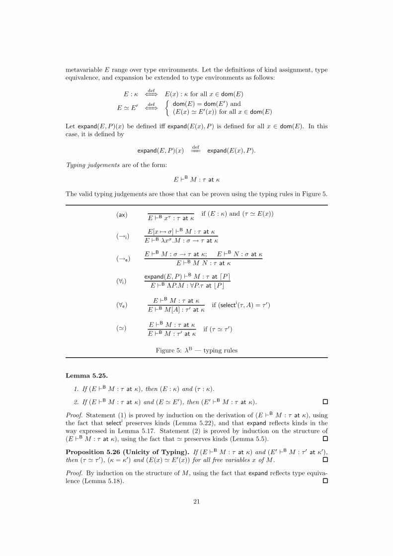
Typing judgements are of the form:

E `B M : τ at κ

The valid typing judgements are those that can be proven using the typing rules in Figure 5.

(ax)E `B xτ : τ at κ

if (E : κ) and (τ ' E(x))

(→i)E[x 7→ σ] `B M : τ at κ

E `B λxσ .M : σ → τ at κ

(→e)E `B M : σ → τ at κ; E `B N : σ at κ

E `B M N : τ at κ

(∀i)expand(E, P ) `B M : τ at dP e

E `B ΛP.M : ∀P.τ at bP c

(∀e)E `B M : τ at κ

E `B M [A] : τ ′ at κif (selecti(τ, A) = τ ′)

(')E `B M : τ at κ

E `B M : τ ′ at κif (τ ' τ ′)

Figure 5: λB — typing rules

Lemma 5.25.

1. If (E `B M : τ at κ), then (E : κ) and (τ : κ).

2. If (E `B M : τ at κ) and (E ' E′), then (E′ `B M : τ at κ).

Proof. Statement (1) is proved by induction on the derivation of (E `B M : τ at κ), usingthe fact that selecti preserves kinds (Lemma 5.22), and that expand reflects kinds in theway expressed in Lemma 5.17. Statement (2) is proved by induction on the structure of(E `B M : τ at κ), using the fact that ' preserves kinds (Lemma 5.5).

Proposition 5.26 (Unicity of Typing). If (E `B M : τ at κ) and (E′ `B M : τ ′ at κ′),then (τ ' τ ′), (κ = κ′) and (E(x) ' E′(x)) for all free variables x of M .

Proof. By induction on the structure of M , using the fact that expand reflects type equiva-lence (Lemma 5.18).

21

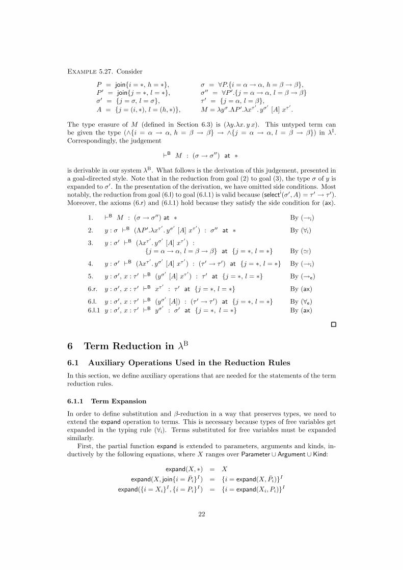
Example 5.27. Consider

P = join{i = ∗, h = ∗}, σ = ∀P.{i = α → α, h = β → β},P ′ = join{j = ∗, l = ∗}, σ′′ = ∀P ′.{j = α → α, l = β → β}σ′ = {j = σ, l = σ}, τ ′ = {j = α, l = β},

A = {j = (i, ∗), l = (h, ∗)}, M = λyσ .ΛP ′.λxτ ′

. yσ′

[A] xτ ′

.

The type erasure of M (defined in Section 6.3) is (λy.λx. y x). This untyped term canbe given the type (∧{i = α → α, h = β → β} → ∧{j = α → α, l = β → β}) in λI.Correspondingly, the judgement

`B M : (σ → σ′′) at ∗

is derivable in our system λB. What follows is the derivation of this judgement, presented ina goal-directed style. Note that in the reduction from goal (2) to goal (3), the type σ of y isexpanded to σ′. In the presentation of the derivation, we have omitted side conditions. Mostnotably, the reduction from goal (6.l) to goal (6.l.1) is valid because (selecti(σ′, A) = τ ′ → τ ′).Moreover, the axioms (6.r) and (6.l.1) hold because they satisfy the side condition for (ax).

1. `B M : (σ → σ′′) at ∗ By (→i)

2. y : σ `B (ΛP ′.λxτ ′

. yσ′

[A] xτ ′

) : σ′′ at ∗ By (∀i)

3. y : σ′ `B (λxτ ′

. yσ′

[A] xτ ′

) :{j = α → α, l = β → β} at {j = ∗, l = ∗} By (')

4. y : σ′ `B (λxτ ′

. yσ′

[A] xτ ′

) : (τ ′ → τ ′) at {j = ∗, l = ∗} By (→i)

5. y : σ′, x : τ ′ `B (yσ′

[A] xτ ′

) : τ ′ at {j = ∗, l = ∗} By (→e)

6.r. y : σ′, x : τ ′ `B xτ ′

: τ ′ at {j = ∗, l = ∗} By (ax)

6.l. y : σ′, x : τ ′ `B (yσ′

[A]) : (τ ′ → τ ′) at {j = ∗, l = ∗} By (∀e)

6.l.1 y : σ′, x : τ ′ `B yσ′

: σ′ at {j = ∗, l = ∗} By (ax)

6 Term Reduction in λB

6.1 Auxiliary Operations Used in the Reduction Rules

In this section, we define auxiliary operations that are needed for the statements of the termreduction rules.

6.1.1 Term Expansion

In order to define substitution and β-reduction in a way that preserves types, we need toextend the expand operation to terms. This is necessary because types of free variables getexpanded in the typing rule (∀i). Terms substituted for free variables must be expandedsimilarly.

First, the partial function expand is extended to parameters, arguments and kinds, in-ductively by the following equations, where X ranges over Parameter ∪ Argument ∪ Kind:

expand(X, ∗) = X

expand(X, join{i = Pi}I) = {i = expand(X, Pi)}

I

expand({i = Xi}I , {i = Pi}

I) = {i = expand(Xi, Pi)}I

22

Now, the partial function expand is inductively extended to terms:

expand(ΛP ′.M, P ) = Λ(expand(P ′, P )). expand(M, P )

expand(M [A], P ) = (expand(M, P ))[expand(A, P )]

expand(λxτ .M, P ) = λxexpand(τ,P ). expand(M, P )

expand(M N, P ) = (expand(M, P )) (expand(N, P ))

expand(xτ , P ) = xexpand(τ,P )

Example 6.1. Consider the term N = ΛP.λxτ .xτ , where P = join{i = ∗, h = ∗} and τ ={i = α, h = β}. Its type erasure (defined in Section 6.3) is λx.x. Its type is

σ = ∀P.{i = α → α, h = β → β}.

Expanding N by the parameter P ′ = join{j = ∗, l = ∗} results in this:

expand(N, P ′) = Λ {j = P, l = P} .λx{j=τ, l=τ}.x{j=τ, l=τ}

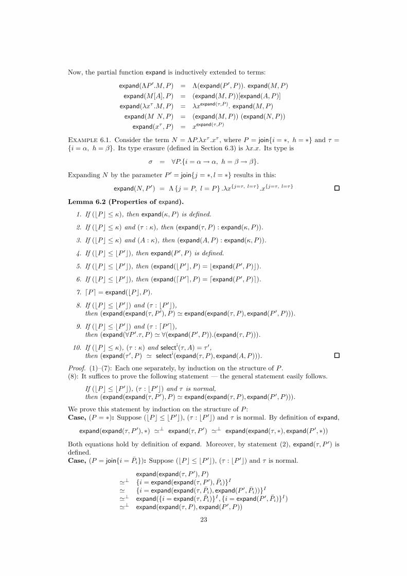
Lemma 6.2 (Properties of expand).

1. If (bP c ≤ κ), then expand(κ, P ) is defined.

2. If (bP c ≤ κ) and (τ : κ), then (expand(τ, P ) : expand(κ, P )).

3. If (bP c ≤ κ) and (A : κ), then (expand(A, P ) : expand(κ, P )).

4. If (bP c ≤ bP ′c), then expand(P ′, P ) is defined.

5. If (bP c ≤ bP ′c), then (expand(bP ′c, P ) = bexpand(P ′, P )c).

6. If (bP c ≤ bP ′c), then (expand(dP ′e, P ) = dexpand(P ′, P )e).

7. dP e = expand(bP c, P ).

8. If (bP c ≤ bP ′c) and (τ : bP ′c),then (expand(expand(τ, P ′), P ) ' expand(expand(τ, P ), expand(P ′, P ))).

9. If (bP c ≤ bP ′c) and (τ : dP ′e),then (expand(∀P ′.τ, P ) ' ∀(expand(P ′, P )).(expand(τ, P ))).

10. If (bP c ≤ κ), (τ : κ) and selecti(τ, A) = τ ′,then (expand(τ ′, P ) ' selecti(expand(τ, P ), expand(A, P ))).

Proof. (1)–(7): Each one separately, by induction on the structure of P .(8): It suffices to prove the following statement — the general statement easily follows.

If (bP c ≤ bP ′c), (τ : bP ′c) and τ is normal,then (expand(expand(τ, P ′), P ) ' expand(expand(τ, P ), expand(P ′, P ))).

We prove this statement by induction on the structure of P :Case, (P = ∗): Suppose (bP c ≤ bP ′c), (τ : bP ′c) and τ is normal. By definition of expand,

expand(expand(τ, P ′), ∗) '⊥ expand(τ, P ′) '⊥ expand(expand(τ, ∗), expand(P ′, ∗))

Both equations hold by definition of expand. Moreover, by statement (2), expand(τ, P ′) isdefined.Case, (P = join{i = Pi}): Suppose (bP c ≤ bP ′c), (τ : bP ′c) and τ is normal.

expand(expand(τ, P ′), P )'⊥ {i = expand(expand(τ, P ′), Pi)}

I

' {i = expand(expand(τ, Pi), expand(P ′, Pi))}I

'⊥ expand({i = expand(τ, Pi)}I , {i = expand(P ′, Pi)}

I)'⊥ expand(expand(τ, P ), expand(P ′, P ))

23

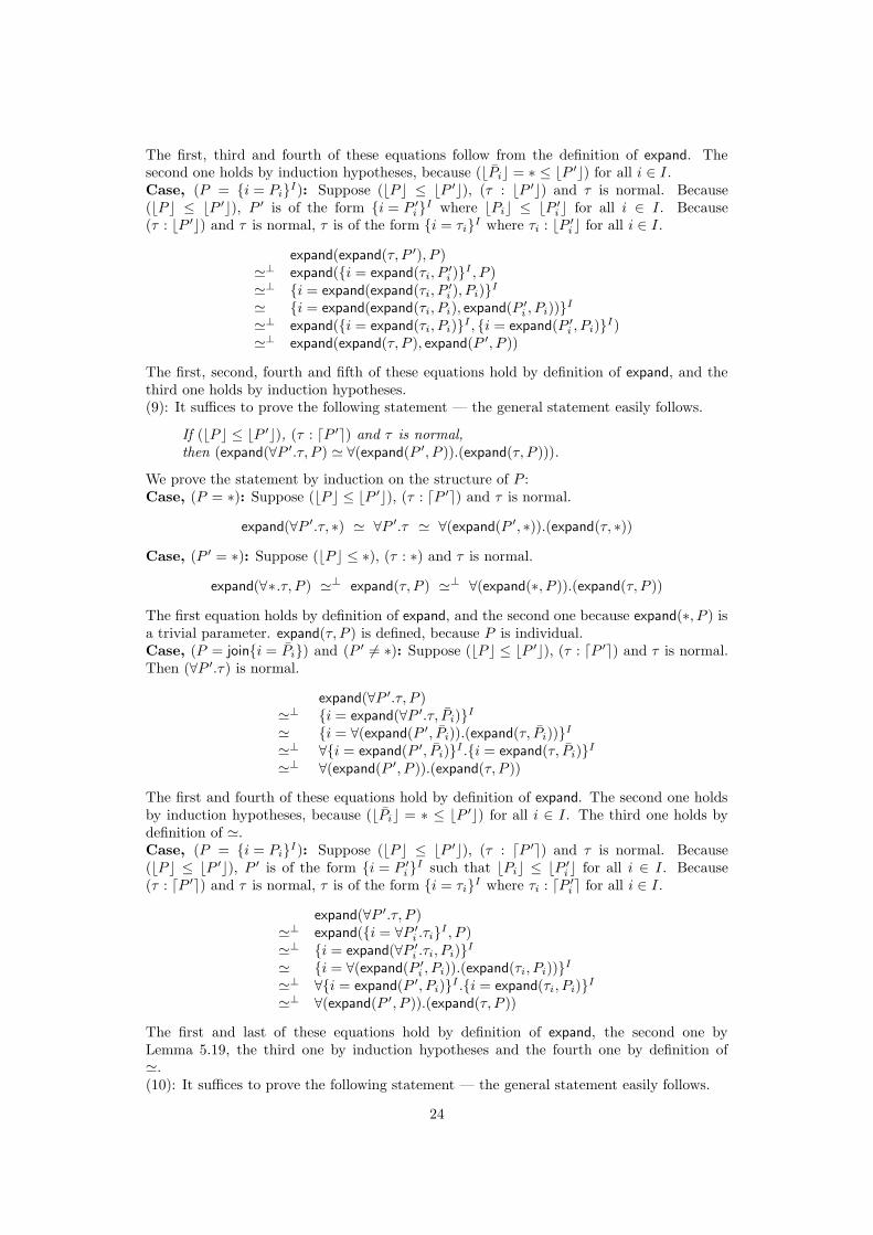
The first, third and fourth of these equations follow from the definition of expand. Thesecond one holds by induction hypotheses, because (bPic = ∗ ≤ bP ′c) for all i ∈ I .Case, (P = {i = Pi}

I): Suppose (bP c ≤ bP ′c), (τ : bP ′c) and τ is normal. Because(bP c ≤ bP ′c), P ′ is of the form {i = P ′

i}I where bPic ≤ bP ′

i c for all i ∈ I . Because(τ : bP ′c) and τ is normal, τ is of the form {i = τi}

I where τi : bP ′i c for all i ∈ I .

expand(expand(τ, P ′), P )'⊥ expand({i = expand(τi, P

′i )}I , P )

'⊥ {i = expand(expand(τi, P′i ), Pi)}

I

' {i = expand(expand(τi, Pi), expand(P ′i , Pi))}

I

'⊥ expand({i = expand(τi, Pi)}I , {i = expand(P ′

i , Pi)}I)

'⊥ expand(expand(τ, P ), expand(P ′, P ))

The first, second, fourth and fifth of these equations hold by definition of expand, and thethird one holds by induction hypotheses.(9): It suffices to prove the following statement — the general statement easily follows.

If (bP c ≤ bP ′c), (τ : dP ′e) and τ is normal,then (expand(∀P ′.τ, P ) ' ∀(expand(P ′, P )).(expand(τ, P ))).

We prove the statement by induction on the structure of P :Case, (P = ∗): Suppose (bP c ≤ bP ′c), (τ : dP ′e) and τ is normal.

expand(∀P ′.τ, ∗) ' ∀P ′.τ ' ∀(expand(P ′, ∗)).(expand(τ, ∗))

Case, (P ′ = ∗): Suppose (bP c ≤ ∗), (τ : ∗) and τ is normal.

expand(∀∗.τ, P ) '⊥ expand(τ, P ) '⊥ ∀(expand(∗, P )).(expand(τ, P ))

The first equation holds by definition of expand, and the second one because expand(∗, P ) isa trivial parameter. expand(τ, P ) is defined, because P is individual.Case, (P = join{i = Pi}) and (P ′ 6= ∗): Suppose (bP c ≤ bP ′c), (τ : dP ′e) and τ is normal.Then (∀P ′.τ) is normal.

expand(∀P ′.τ, P )'⊥ {i = expand(∀P ′.τ, Pi)}

I

' {i = ∀(expand(P ′, Pi)).(expand(τ, Pi))}I

'⊥ ∀{i = expand(P ′, Pi)}I .{i = expand(τ, Pi)}

I

'⊥ ∀(expand(P ′, P )).(expand(τ, P ))

The first and fourth of these equations hold by definition of expand. The second one holdsby induction hypotheses, because (bPic = ∗ ≤ bP ′c) for all i ∈ I . The third one holds bydefinition of '.Case, (P = {i = Pi}

I): Suppose (bP c ≤ bP ′c), (τ : dP ′e) and τ is normal. Because(bP c ≤ bP ′c), P ′ is of the form {i = P ′

i}I such that bPic ≤ bP ′

i c for all i ∈ I . Because(τ : dP ′e) and τ is normal, τ is of the form {i = τi}

I where τi : dP ′i e for all i ∈ I .

expand(∀P ′.τ, P )'⊥ expand({i = ∀P ′

i .τi}I , P )

'⊥ {i = expand(∀P ′i .τi, Pi)}

I

' {i = ∀(expand(P ′i , Pi)).(expand(τi, Pi))}

I

'⊥ ∀{i = expand(P ′, Pi)}I .{i = expand(τi, Pi)}

I

'⊥ ∀(expand(P ′, P )).(expand(τ, P ))

The first and last of these equations hold by definition of expand, the second one byLemma 5.19, the third one by induction hypotheses and the fourth one by definition of'.(10): It suffices to prove the following statement — the general statement easily follows.

24

If (bP c ≤ κ), (τ : κ), (selecti(τ, A) = τ ′) and τ is normal,then (expand(τ ′, P ) ' selecti(expand(τ, P ), expand(A, P ))).

We prove this statement by induction on the structure of P :Case, (P = ∗): Suppose (bP c ≤ κ), (τ : κ), (selecti(τ, A) = τ ′) and τ is normal.

selecti(expand(τ, ∗), expand(A, ∗)) '⊥ selecti(τ, A) = τ ′ ' expand(τ ′, ∗)

The first and the last of these equations follow from the definition of expand.Case, (P = join{i = Pi}): Suppose (bP c ≤ κ), (τ : κ), (selecti(τ, A) = τ ′) and τ is normal.

selecti(expand(τ, P ), expand(A, P ))

'⊥ selecti({i = expand(τ, Pi)}I , {i = expand(A, Pi)}

I)

'⊥ {i = selecti(expand(τ, Pi), expand(A, Pi))}I

' {i = expand(τ ′, Pi)}I

'⊥ expand(τ ′, P )

The first of these equations follows from the definition of expand, the second one from thedefinition of selecti, and the last one follows from the definition of expand. The third oneholds by induction hypotheses, because (bPic = ∗ ≤ κ) for all i ∈ I .Case, (P = {i = Pi}

I): Suppose (bP c ≤ κ), (τ : κ), (selecti(τ, A) = τ ′) and τ is normal.Because (bP c ≤ κ), κ is of the form {i = κi}

I such that (bPic ≤ κi) for all i ∈ I . Because(τ : κ) and τ is normal, τ is of the form {i = τi}

I where τi : κi for all i ∈ I . Because(selecti(τ, A) = τ ′), A and τ ′ are of the forms (τ ′ = {i = τ ′

i}I) and (A = {i = Ai}

I) suchthat (selecti(τi, Ai) = τ ′

i ) for all i ∈ I .

selecti(expand(τ, P ), expand(A, P ))

'⊥ selecti({i = expand(τi, Pi)}I , {i = expand(Ai, Pi)}

I)

'⊥ {i = selecti(expand(τi, Pi), expand(Ai, Pi))}I

' {i = expand(τ ′i , Pi)}

I

'⊥ expand(τ ′, P )

The first of these equations follows from the definition of expand, the second one from thedefinition of selecti, the third one holds by induction hypotheses, and the last one followsfrom the definition of expand.

Lemma 6.3. If (E `B M : τ at κ) and (bP c ≤ κ),then (expand(E, P ) `B expand(M, P ) : expand(τ, P ) at expand(κ, P )).

Proof. By induction on the derivation of (E `B M : τ at κ) The interesting cases are theones for ΛP -abstraction and [A]-application:Case:

expand(E, P ′) `B M : τ at dP ′e

E `B ΛP ′.M : ∀P ′.τ at bP ′c

bP c ≤ bP ′c AssumptionbP c ≤ dP ′e By bP ′c ≤ dP ′e and transitivity of ≤expand(expand(E, P ′), P )

`B expand(M, P ) : expand(τ, P ) at expand(dP ′e, P ) By ind. hyp.expand(expand(E, P ), expand(P ′, P ))

`B expand(M, P ) : expand(τ, P ) at dexpand(P ′, P )eBy Lemma 6.2, (8) and (6)

expand(E, P )`B expand(ΛP ′.M, P ) : ∀(expand(P ′, P )).(expand(τ, P )) at bexpand(P ′, P )c

By (∀i) and definition of expand for termsexpand(E, P )

25

`B expand(ΛP ′.M, P ) : expand(∀P ′.τ, P ) at expand(bP ′c, P )By Lemma 6.2, (9) and (5)

Case:E `B M : τ at κ

E `B M [A] : τ ′ at κif (selecti(τ, A) = τ ′)

bP c ≤ κ Assumptionexpand(E, P ) `B expand(M, P ) : expand(τ, P ) at expand(κ, P ) By ind. hyp.selecti(expand(τ, P ), expand(A, P )) ' expand(τ ′, P ) By Lemma 6.2 (10)expand(E, P ) `B expand(M [A], P ) : expand(τ ′, P ) at expand(κ, P )

By (∀e) and definition of expand for terms

Corollary 6.4. If (E `B M : τ at bP c),then (expand(E, P ) `B expand(M, P ) : expand(τ, P ) at dP e).

Proof. Follows from Lemma 6.3 and Lemma 6.2 (7).

6.1.2 Substitution

Let a substitution be a finite function from Var to Term. Let s range over substitutions. Letthe operation expand be extended to act as a partial function on substitutions as follows.Let expand(s, P ) be defined iff expand(s(x), P ) is defined for all x ∈ dom(s). In this case, letit be defined by:

expand(s, P )(x) = expand(s(x), P )

Let the application of a substitution s to a term M be defined inductively by the followingequations.

s(ΛP.M) = ΛP.(expand(s, P )(M))

s(M [A]) = (s(M))[A]

s(λxτ .M) = λxτ .(s(M)), if x does not occur freely in ran(s) and x 6∈ dom(s)

s(M N) = s(M) s(N)

s(xτ ) = s(x), if x ∈ dom(s)

s(xτ ) = xτ , if x 6∈ dom(s)

Let M [x := N ] be the term that results from applying the singleton substitution {(x, N)}to M .

Example 6.5. Let N , P , P ′, τ and σ be as in Example 6.1. Consider the term

M = ΛP ′.λxτ ′

. yσ′

[A] xτ ′

where τ ′ = {j = α, l = β}, σ′ = {j = σ, l = σ} and A = {j = (i, ∗), l = (h, ∗)}. This termis well typed in the type environment {(y, σ)}. Its type erasure (defined in Section 6.3) is(λx. y x). Substituting N for y in M results in

M [y := N ] = ΛP ′.((λxτ ′

. yσ [A] xτ ′

)[y := expand(N, P ′)])

= ΛP ′.λxτ ′

. (expand(N, P ′)) [A] xτ ′

= ΛP ′.λxτ ′

. (Λ{j = P, l = P}.λx{j=τ, l=τ}.x{j=τ, l=τ}) [A] xτ ′

Let typing judgements for substitutions be defined as follows:

(E′ `B s : E at κ) ⇐def=⇒ (E′ `B s(xE(x)) : E(x) at κ) for all x ∈ dom(E)

26

Lemma 6.6. If (E′ `B s : E at bP c),then (expand(E ′, P ) `B expand(s, P ) : expand(E, P ) at dP e).

Proof. This follows from Corollary 6.4.

Lemma 6.7. If (E `B M : τ at κ) and (E′ `B s : E at κ),then (E′ `B s(M) : τ at κ).

Proof. By induction on the derivation of (E `B M : τ at κ), using Lemma 6.6.

6.1.3 Selection for Terms

The preceding treatment of substitution prepares for the definition of β-reduction of terms ofthe form ((λxτ .M)N). We also need to define reduction of terms of the form (ΛP.M)[A]. Tothis end, we extend selectb to parameters, arguments and kinds, inductively by the followingequations, where X ranges over Parameter ∪ Argument ∪ Kind:

selectb(X, ∗) = X

selectb({i = Xi}I , (j, A)) = selectb(Xj , A), if j ∈ I

selectb({i = Xi}I , {i = Ai}

I) = {i = selectb(Xi, Ai)}I

The partial function selectb is inductively extended to terms:

selectb(ΛP ′.M, A) = Λ(selectb(P ′, A)). selectb(M, A)

selectb(M [A′], A) = (selectb(M, A))[selectb(A′, A)]

selectb(λxτ .M, A) = λxselectb(τ,A). selectb(M, A)

selectb(M N, A) = (selectb(M, A)) (selectb(N, A))

selectb(xτ , A) = xselectb(τ,A)

Finally, let selectb be extended to environments as follows. Let selectb(E, A) be defined iffselect

b(E(x), A) is defined for all x ∈ dom(E). In this case, let it be defined by

selectb(E, A)(x) = selectb(E(x), A).

Lemma 6.8 (Properties of selectb).

1. (A / κ) if and only if selectb(κ, A) is defined.

2. If (A / κ) and (τ : κ), then (selectb(τ, A) : selectb(κ, A)).

3. If (A / κ) and (A′ : κ), then (selectb(A′, A) : selectb(κ, A)).

4. If (A / bP c), then selectb(P, A) is defined.

5. If (A / bP c), then (bselectb(P, A)c = selectb(bP c, A)).

6. If (A / bP c), then (dselectb(P, A)e = selectb(dP e, A)).

7. If (A / bP c) and (τ : bP c),then (selectb(expand(τ, P ), A) ' expand(selectb(τ, A), selectb(P, A))).

8. If (A / bP c) and (τ : dP e),then (selectb(∀P.τ, A) ' ∀(selectb(P, A)).selectb(τ, A)).

9. If (A / κ), (τ : κ) and (selecti(τ, A′) = τ ′),then (selectb(τ ′, A) ' selecti(selectb(τ, A), selectb(A′, A))).

27

Proof. Statements (1) through (6) are all proved, separately, by induction on the structureof A. Statements (7) through (9) are proved similarly to statements (8) through (10) ofLemma 6.2.

Lemma 6.9. If (E `B M : τ at κ) and (A / κ),then (selectb(E, A) `B selectb(M, A) : selectb(τ, A) at selectb(κ, A)).

Proof. By induction on the derivation of (E `B M : τ at κ), using Lemma 6.8.

6.1.4 Matching Type Selection Parameters and Arguments

We define a partial function match from Parameter × Argument to Parameter × Argument ×Argument. This function will be needed for the reduction rule (βΛ) for type selection. The(βΛ)-reduction rule will apply to redexes of the form (ΛP.M)[A]. The match(P, A) operationattempts to match the argument A against the type selection parameter P . It splits A intotwo parts — the selectb-argument As that will be fed to selectb(M, · ), and the remainder Ar

that will be pushed below the Λ. The partial function match is defined inductively by thefollowing rules. In the second rule, note that dP e is a trivial type selection argument for alltype selection parameters P .

match(∗, A) = (∗, ∗, A) match(P , ∗) = (P , ∗, dPe)

match(Pj , A) = (P ′, As, Ar)

match(join{i = Pi}I , (j, A)) = (P ′, (j, As), Ar)if j ∈ I

match(Pi, Ai) = (P ′i , A

si, A

ri) for all i ∈ I

match({i = Pi}I , {i = Ai}I) = ({i = P ′i}

I , {i = Asi}

I , {i = Ari}

I)

Lemma 6.10 (Properties of match). Let match(P, A) = (P ′, As, Ar). Then:

1. (bP c = bP ′c).

2. (dP ′e = selectb(dP e, As)).

3. (Ar : dP ′e).

4. (As / dP e).

5. If (τ : dP e), then (selecti(∀P.τ, A) '⊥ ∀P ′.selecti(selectb(τ, As), Ar)).

6. If (τ : bP c), then (selectb(expand(τ, P ), As) ' expand(τ, P ′)).

Proof. Statements (1) through (4) are proved, separately, by induction on the derivation of(match(P, A) = (P ′, As, Ar)).(5): By induction on the derivation of (match(P, A) = (P ′, As, Ar)).Case.

match(∗, A) = (∗, ∗, A)

Suppose (τ : ∗).

selecti(∀∗.τ, A)

'⊥ selecti(τ, A)

'⊥ selecti(selectb(τ, ∗), A)

'⊥ ∀∗.selecti(selectb(τ, ∗), A)

28

The first equation holds by definition of selecti, the second one by definition of selectb andthe third one by definition of '.Case.

match(P , ∗) = (P , ∗, dPe)

Suppose (τ : dPe).

selecti(∀P .τ, ∗)' ∀P .τ

' ∀P .selecti(τ, dP e)

' ∀P .selecti(selectb(τ, ∗), dP e)

The first equation holds by definition of selecti and the third one by definition of selectb.The second equation holds by Lemma 5.24, because dP e is a trivial argument.Case.



Let (P = join{i = Pi}I). Suppose (τ : dP e). Then τ is such that τ ' {i = τi}

I where(τi : dPie) for all i ∈ I .

selecti(∀P.τ, (j, A))

'⊥ selecti(∀Pj .τj , A)

'⊥ ∀P ′.selecti(selectb(τj , As), Ar)

'⊥ ∀P ′.selecti(selectb(τ, (j, As)), Ar)

The first and third equation hold by Lemma 5.23, and the second one by induction hypothe-ses.Case.


si, A

ri) for all i ∈ I


I , {i = Asi}

I , {i = Ari}

I)

Let (P = {i = Pi}I) and (P ′ = {i = P ′

i }I). Suppose (τ : dP e). Then τ is such that

τ ' {i = τi}I where (τi : dPie) for all i ∈ I .

selecti(∀P.τ, {i = Ai}I)

'⊥ selecti({i = ∀Pi.τi}

I , {i = Ai}I)

'⊥ {i = selecti(∀Pi.τi, Ai)}I

'⊥ {i = ∀P ′i .select

i(selectb(τi, Asi), A

ri)}

I

'⊥ ∀P ′.{i = selecti(selectb(τi, Asi), A

ri)}

I

'⊥ ∀P ′.selecti({i = selectb(τi, Asi)}

I , Ar)

'⊥ ∀P ′.selecti(selectb(τ, As), Ar)

The first equation holds by definition of selecti, the second, fifth and sixth one by Lemma 5.23,the third one by induction hypothesis and the fourth one by definition of '.(6): By induction on the derivation of (match(P, A) = (P ′, As, Ar)).Case.

match(∗, A) = (∗, ∗, A)

Suppose (τ : ∗). Then (selectb(expand(τ, ∗), ∗) ' expand(τ, ∗)), by definition of selectb.Case.

match(P , ∗) = (P , ∗, dPe)

Suppose (τ : ∗). Then (selectb(expand(τ, P ), ∗) '⊥ expand(τ, P )), by definition of selectb.Moreover, expand(τ, P ) is defined because P is an individual parameter.Case.



29

Let (P = join{i = Pi}I). Suppose (τ : ∗).

selectb(expand(τ, P ), (j, As))

'⊥ selectb({i = expand(τ, Pi)}I , (j, As))

'⊥ selectb(expand(τ, Pj), As)' expand(τ, P ′)

The first equation holds by definition of expand, the second one by definition of selectb, andthe third one by induction hypotheses.Case.


si, A

ri) for all i ∈ I


I , {i = Asi}

I , {i = Ari}

I)

Let (P = {i = Pi}I) and (As = {i = As

i}I). Suppose (τ : bP c). Then τ is such that

τ ' {i = τi}I where (τi : bPic) for all i ∈ I .

selectb(expand(τ, P ), As)

'⊥ selectb({i = expand(τi, Pi)}I , As)

'⊥ {i = selectb(expand(τi, Pi), Asi)}

I

' {i = expand(τi, P′i )}I

'⊥ expand(τ, P ′)

The first and fourth equation hold by Lemma 5.19, the second one by definition of selectb,

and the third one by induction hypotheses.

6.2 Reduction Rules for Terms

Let a binary relation R ⊆ Term×Term be called compatible iff it satisfies the following rules:

(M R N) ⇒ ((ΛP.M) R (ΛP.N))(M R N) ⇒ ((M [A]) R (N [A]))(M R N) ⇒ ((λxτ .M) R (λxτ .N))(M R N) ⇒ ((M M ′) R (N M ′))(M R N) ⇒ ((M ′ M) R (M ′ N))

Definition 6.11 (Term Reduction). Let → be the least compatible relation R thatcontains all instances of the rules (βλ), (βΛ), (∗P ) and (∗A), below.

(βλ) ((λxτ .M)N) R (M [x := N ])

(βΛ) (ΛP.M)[A] R ΛP ′.((selectb(M, As))[Ar]),if match(P, A) = (P ′, As, Ar) and neither P nor A is trivial

(∗P ) (ΛP.M) R M, if P is trivial(∗A) (M [A]) R M, if A is trivial

Example 6.12. Let the terms M and N and the type σ be as in Example 6.5. Considerthis term:

M ′ = (λyσ . M) N

This term is well typed. Its type erasure (defined in Section 6.3) is ((λy.λx. y x) (λx.x)).The term M ′ reduces, by a βλ-reduction step, to the term

ΛP ′.λxτ ′

. (Λ {j = P, l = P} .λx{j=τ, l=τ}.x{j=τ, l=τ}) [A] xτ ′

,

where P , P ′, τ , τ ′ and A are as in Example 6.5.

30

Example 6.13. Consider the term M = (ΛP1.ΛP2.λxτ .x)[A], where

P1 = {m = join{j = ∗, k = ∗}, n = ∗},P2 = {m = ∗, n = join{h = ∗, l = ∗}},A = {m = ∗, n = (h, ∗)},τ = {m = {j = α1, k = α2}, n = {h = β1, l = β2}}.

The term M first reduces to ΛP1.(ΛP2.λxτ .x)[A], by a (βΛ)-step, where P1 and A passthrough each other without interacting. By another (βΛ)-step, it reduces to ΛP1.ΛP ′

2.(λxσ .x)[A′]where

P ′2 = {m = ∗, n = ∗},

A′ = {m = ∗, n = ∗},σ = {m = {j = α1, k = α2}, n = β1}.

Finally, it reduces to ΛP1.λxσ .x, removing the trivial P ′2 and A′ by a (∗P )-step and a (∗A)-

step.

Theorem 6.14 (Subject Reduction). If (M → N) and (E `B M : τ at κ),then (E `B N : τ at κ).

Proof. By induction on the proof tree of (M → N). For (βλ), one uses Lemma 6.7. For(∗A) and (∗P ), one uses Lemma 5.24. Here is the proof for (βΛ). Assume the following:

(E `B (ΛP.M)[A] : τ at κ) and (match(P, A) = (P ′, As, Ar))

From the first of these assumptions, by inversion of the typing rules, there is a τ ′ such that

(E `B (ΛP.M) : τ ′ at κ) and (selecti(τ ′, A) ' τ)

From the first of these statements, by another inversion of the typing rules, there is a τ ′′

such that

(expand(E, P ) `B M : τ ′′ at dP e) and (τ ′ ' ∀P.τ ′′) and (κ = bP c)

By Lemma 6.10 (4), it is the case that (As / dP e). Therefore, by Lemma 6.9:

selectb(expand(E, P ), As)

`B selectb(M, As) : selectb(τ ′′, As) at selectb(dP e, As)

By Lemma 6.10 (2), it is the case that (selectb(dP e, As) = dP ′e). Therefore,

selectb(expand(E, P ), As) `B selectb(M, As) : selectb(τ ′′, As) at dP ′e

By Lemma 6.10 (5), it is the case that (∀P ′.selecti(selectb(τ ′′, As), Ar) '⊥ τ). In particular,selecti(selectb(τ ′′, As), Ar) is defined. Let σ = selecti(selectb(τ ′′, As), Ar). Then, by (∀e),

selectb(expand(E, P ), As) `B (selectb(M, As))[Ar] : σ at dP ′e

By Lemma 6.10 (6), it is the case that (selectb(expand(E, P ), As) ' expand(E, P ′)). There-fore,

expand(E, P ′) `B (selectb(M, As))[Ar] : σ at dP ′e

Then, by (∀i),E `B ΛP ′.(selectb(M, As))[Ar] : ∀P ′.σ ' τ at bP ′c

By Lemma 6.10 (1), it is the case that (bP ′c = κ). Therefore,

E `B ΛP ′.(selectb(M, As))[Ar] : τ at κ.

31

6.3 Correspondence of Typed and Untyped Reduction

Substitution for untyped terms is defined as usual, and so is β-reduction:

(β) (λx.M)N → M [x := N ]

Let →∗ denote the reflexive and transitive closure of →. We define a map | · | from Term toUntypedTerm that erases type-annotations:

|ΛP.M | = |M ||M [A]| = |M |

|λxτ .M | = λx.|M ||MN | = |M | |N |

|xτ | = x

Lemma 6.15.

1. If expand(M, P ) is defined, then (|expand(M, P )| = |M |).

2. If M [x := N ] is defined, then |M [x := N ]| = |M |[x := |N |].

3. If selectb(M, A) is defined, then (|selectb(M, A)| = |M |).

Proof. All statements, separately and in this order, by induction on the size of M .

Theorem 6.16 (Soundness of Reduction).If M, N ∈ Term and M → N , then |M | →∗ |N |.

Proof. Obvious from the previous lemma.

Lemma 6.17.

1. Any sequence of (βΛ), (∗P ) and (∗A) reduction steps is terminating.

2. If M reduces to N by (βΛ), (∗P ) or (∗A) reduction, then |M | = |N |.

3. If selecti(∀P.τ, A) is defined, then so is match(P, A).

4. A well typed term that is free of (βΛ), (∗P ) or (∗A) redexes is of the form

ΛP1 . . . ΛPn.M [A1] . . . [Am]

where n, m ≥ 0, the Pi’s and Ai’s are not trivial, and M is either a variable, a λ-abstraction or an application.

5. If (∀P.τ ′ ' τ → σ), then P is trivial.

6. If selecti(τ → σ, A) is defined, then A is trivial.

Proof. To prove statement (1), define a weight function like this:

‖M‖ =

(no. of occurrences of join in M)+ (no. of occurrences of Λ in M)+ (no. of occurrences of [·] in M)

An inspection of the reduction rules shows that ‖M‖ > ‖N‖, if M reduces to N by one of(βΛ), (∗P ) and (∗A). Statements (2) is obvious. Statement (3) is proved by induction on thestructure of A, using the fact that P is an individual parameter if ∀P.τ is an individual type.Statement (4) follows from the well-typedness assumption and statement (3). Statement (5)is proved by induction on the structure of P , using that equivalent types have equal normalforms. Statement (6) is proved by induction on the structure of A.

Theorem 6.18 (Completeness of Reduction).If M is well typed and (|M | → N ′),then there is a λB-term N such that (M →∗ N) and (|N | = N ′).

32

Proof. The statement is proved by induction on the proof of (|M | → N ′). The only inter-esting case is when (|M | = (λx.R)S) and (N ′ = R[x := S]). So suppose this is the case.We want to reduce M to a term N such that (|N | = R[x := S]). To this end, first eliminateall (βΛ), (∗P ) and (∗A) redexes from M . This terminates, by the previous lemma. Theresulting term, let’s call it M1, is of the following form:

M1 = ΛP1 . . . ΛPn.(M2 M3)[A1] . . . [Am]

where n, m ≥ 0, the Pi’s and Ai’s are not trivial, (|M2| = λx.R) and (|M3| = S). The termM2 is such that

M2 = ΛP ′1 . . . ΛP ′

k.(λxσ .M4)[A′1] . . . [A′

l]

where k, l ≥ 0, the P ′i ’s and A′

i’s are not trivial and (|M4| = R).We now show that (k = 0): The term M2 must have a function type because (M2 M3)

is well typed. Suppose, towards a contradiction, that (k > 0). Then, M2’s type is equalto (∀P ′

1.τ) for some τ . Because P ′1 is not trivial, this contradicts the fact that M2 has a

function type, by Lemma 6.17 (5).By a similar argument, which uses Lemma 6.17 (6), one shows that l = 0. Now, define

N byN = ΛP1 . . . ΛPn.(M4[x := M3])[A1] . . . [Am]

Then (M →∗ N) and (|N | = R[x := S]).

7 Relating Branching Types to Intersection Types

7.1 From Branching Types to Intersection Types

Individual λB-types are closely related to to types of the intersection type system λI fromSection 2.2. A λI-type is obtained from an individual λB-type by first normalizing the λB-type and then erasing all type selection parameters. Formally, we define a function | · | thatmaps individual λB-types to λI-types inductively by the following equations:

|α| = α

|µ → ν| = |µ| → |ν||∀join{i = Pi}

I .{i = µi}I | = ∧{i = |∀Pi.µi|}

I

|τ | = |nf(τ)| if ¬normal(τ)

The function is extended to environments by |E|(x) = |E(x)|.

Theorem 7.1 (Soundness of | · |, Special Version). If (E `B M : τ at ∗), then (|E| `i

|M | : |τ |).

In the remainder of this section, we will prove this theorem. Note that the theorem onlymakes a claim about individual λB-typings. The theorem is a corollary of a more generaltheorem that applies to arbitrary λB-typings. To formulate this more general soundnesstheorem, we need to make some definitions.

Definition 7.2 (Maximal Paths of Kinds). An individual argument A is called a max-imal path of a kind κ, if (selectb(κ, A) = ∗). We write (A � κ) iff A is a maximal path of κ.Maxpath(κ) denotes the set of all maximal paths of κ.

Lemma 7.3.

1. If (A � κ), then (A / κ).

2. If (A � dPe), then (selectb(expand(τ, P ), A) ' τ).

Proof. (1) is proved by induction on the structure of A, and (2) by induction on the structureof P .

33

The function selectb is extended to a partial function from environments to environmentsas follows: selectb(E, A) is defined iff selectb(E(x), A) is defined for all x ∈ dom(E). In thatcase, it is defined by selectb(E, A) (x) = selectb(E(x), A).

Theorem 7.4 (Soundness of | · |, General Version).If (E `B M : τ at κ) and (A � κ), then (|selectb(E, A)| ì |M | : |selectb(τ, A)|).

Proof of Theorem 7.1. Follows from Theorem 7.4, because (∗ � ∗), (selectb(E, ∗) ' E) and(selectb(τ, ∗) ' τ).

The remainder of this section is devoted to the proof of Theorem 7.4. The proof is bylexicographical induction on the pair 〈size(M), size(κ)〉, where size is defined as follows:

size : Term → N

size(xτ ) = 0, size(λxτ .M) = size(M) + 1,

size(M N) = size(M) + size(N) + 1, size(ΛP.M) = size(M) + 1,

size(M [A]) = size(M) + 1.

size : Kind → N

size(∗) = 0, size({i = κi}I) = Max{ size(κi) i ∈ I } + 1.

Lemma 7.5. If (selectb(M, A) = N), then (size(M) = size(N)).

Lemma 7.6. selectb(τ, (i, A)) '⊥ selectb(selectb(τ, (i, ∗)), A).

Part (2) of the following lemma simulates the (∀e)-rule on λI-typing-judgements. Part(1) simulates an instance of the (∀i)-rule. (The simulation of this instance suffices for theproof of Theorem 7.4.)

Lemma 7.7.

1. If (τ : dPe) and (E ì M : |selectb(τ, A)|) for all A ∈ Maxpath(dP e),then (E ì M : |∀P .τ |).

2. If (E ì M : |τ |) and (selecti(τ, A) ' τ ′), then (E ì M : |τ ′|).

Proof. (1): It suffices to prove the statement for normal τ . So suppose that this is the case.The proof is by induction on the structure of P .Case, P = ∗: Suppose (τ : ∗) and (E ì M : |selectb(τ, A)|) for all A ∈ Maxpath(∗). Because(∗ ∈ Maxpath(∗)), it is then the case that (E ì M : |selectb(τ, ∗)|). But (selectb(τ, ∗) ' ∀∗.τ).Case, P = join{i = Pi}

I : Suppose (τ : dP e) and (E ì M : |selectb(τ, A)|) for all A ∈Maxpath(dP e). Because we assumed τ normal, it holds that τ = {i = τi}

I where τi : dPiefor all i ∈ I .

Claim: (E ì M : |selectb(τi, A)|) for all i ∈ I and all A in Maxpath(dPie). To provethis claim, suppose that i ∈ I and A ∈ Maxpath(dPie). Then (i, A) ∈ Maxpath(dP e). Then(E ì M : |selectb(τ, (i, A))|), by assumption. But (selectb(τ, (i, A)) = selectb(τi, A)).

Now, by induction hypotheses, (E ì M : |∀Pi.τi|) for all i ∈ I . Then (E ì M : ∧{i =|∀Pi.τi|}

I), by (∧i). But (∧{i = |∀Pi.τi|}I = |∀P .τ |).

(2): By induction on the structure of A.Case, A = ∗: Suppose (E ì M : |τ |) and (selecti(τ, ∗) ' τ ′). Then (τ ′ ' τ) and, therefore,(E ì M : |τ ′|).Case, A = (j, A′): Suppose (E ì M : |τ |) and (selecti(τ, A) ' τ ′). Then there are I , (Pi)i∈I ,(τi)i∈I such that (j ∈ I) and (nf(τ) = ∀join{i = Pi}

I .{i = τi}I) and (selecti(∀Pj .τj , A

′) ' τ ′).Moreover, (|τ | = ∧{i = |∀Pi.τi|}

I), by definition of | · |. Then (E ì M : |∀Pj .τj |), by (∧e).Then (E ì M : |τ ′|), by induction hypotheses.

34

Proof of Theorem 7.4. The proof is by lexicographical induction on the pair 〈size(M), size(κ)〉.Suppose (E `B M : τ at κ) and (A � κ).Case, κ = {i = κi}

I: By definition of �, there are A′ and i in I such that (κ = (i, A′)) and(A′ � κi). By Lemmas 7.3(1) and 6.9,

selectb(E, (i, ∗)) `B selectb(M, (i, ∗)) : selectb(τ, (i, ∗)) at κi

By Lemma 7.5, (size(selectb(M, (i, ∗))) = size(M)). Therefore, by induction hypotheses andLemma 6.15,

|selectb(selectb(E, (i, ∗)), A′)| ì |M | : |selectb(selectb(τ, (i, ∗)), A′)|

Then, by Lemma 7.6,|selectb(E, A)| ì |M | : |selectb(τ, A)|

Case, κ = ∗: Because (A � ∗), it is the case that (A = ∗). Because (selectb(E, ∗) = E)and (selectb(τ, ∗) = τ), we have to show that (|E| ì |M | : |τ |). We distinguish cases bythe outermost term constructor of M . The cases where M is a variable, λ-abstraction orapplication are straightforward.Subcase, M = ΛP .N : By inversion of the typing rule for Λ, there is a type σ such that(τ ' ∀P .σ) and

expand(E, P ) `B N : σ at dP e

By induction hypothesis,

(∀A ∈ Maxpath(dP e)) (|selectb(expand(E, A), P )| ì |N | : |selectb(σ, A)|)

Then, by Lemma 7.3(2),

(∀A ∈ Maxpath(dP e)) (|E| ì |N | : |selectb(σ, A)|)

Then (E ì |M | : τ), by Lemma 7.7(1).Subcase, M = N [A]: By inversion of the typing rule for type selection application, there isa type σ such that (selecti(σ, A) ' τ) and (E `B N : σ at ∗). Then, by induction hypothesis,(|E| ì |N | : |σ|). Then (|E| ì |M | : |τ |), by Lemma 7.7(2).

7.2 From Intersection Types to Branching Types

We definee : IntTy → IndTy

e(α) = α

e(τ → σ) = e(τ) → e(σ)e(∧{i = τi}

I) = ∀join{i = ∗}I .{i = e(τi)}I

The function is extended to environments by e(E)(x) = e(E(x)).

Theorem 7.8. If (E ì M : τ), then there is a λB-term N such that |N | = M and(e(E) `B N : e(τ) at ∗).

Proof. Straightforward induction on the derivation of (E ì M : τ).

References

[AB91] F. Alessi and F. Barbanera. Strong conjunction and intersection types. InA. Tarlecki, editor, Proc. 16th Int’l Symp. Mathematical Foundations Com-puter Science (MFCS ’91), volume 520 of LNCS, pages 64–73. Springer-Verlag,1991.

35

[AT00] Torben Amtoft and Franklyn Turbak. Faithful translations between polyvari-ant flows and polymorphic types. In Programming Languages & Systems, 9thEuropean Symp. Programming, volume 1782 of LNCS, pages 26–40. Springer-Verlag, 2000.

[Ban97] Anindya Banerjee. A modular, polyvariant, and type-based closure analysis.In ICFP ’97 [ICFP97].

[BM94] Franco Barbanera and Simone Martini. Proof-theoretical connectives and re-alizability. Arch. Math. Logic, 33:189–211, 1994.

[CDC80] Mario Coppo and Mariangiola Dezani-Ciancaglini. An extension of the ba-sic functionality theory for the λ-calculus. Notre Dame J. Formal Logic,21(4):685–693, 1980.

[CLV01] Beatrice Capitani, Michele Loreti, and Betti Venneri. Hyperformulae, paralleldeductions and intersection types. Electronic Notes in Theoretical ComputerScience, 50, 2001. Proceedings of ICALP 2001 workshop: Bohm’s Theorem:Applications to Computer Science Theory (BOTH 2001), Crete, Greece, 2001-07-13.

[DCGV97] Mariangiola Dezani-Ciancaglini, Silvia Ghilezan, and Betti Venneri. The“relevance” of intersection and union types. Notre Dame J. Formal Logic,38(2):246–269, Spring 1997.

[DMTW97] Allyn Dimock, Robert Muller, Franklyn Turbak, and J. B. Wells. Stronglytyped flow-directed representation transformations. In ICFP ’97 [ICFP97],pages 11–24.

[DWM+01a] Allyn Dimock, Ian Westmacott, Robert Muller, Franklyn Turbak, and J. B.Wells. Functioning without closure: Type-safe customized function represen-tations for Standard ML. In Proc. 6th Int’l Conf. Functional Programming,pages 14–25. ACM Press, 2001.

[DWM+01b] Allyn Dimock, Ian Westmacott, Robert Muller, Franklyn Turbak, J. B. Wells,and Jeffrey Considine. Program representation size in an intermediate lan-guage with intersection and union types. In Types in Compilation, Third Int’lWorkshop, TIC 2000, volume 2071 of LNCS, pages 27–52. Springer-Verlag,2001.

[DWM+01c] Allyn Dimock, Ian Westmacott, Robert Muller, Franklyn Turbak, J. B. Wells,and Jeffrey Considine. Program representation size in an intermediate lan-guage with intersection and union types. Technical Report BUCS-TR-2001-02,Comp. Sci. Dept., Boston Univ., March 2001. This is a version of [DWM+01b]extended with an appendix describing the CIL typed intermediate language.

[Gir72] J[ean]-Y[ves] Girard. Interpretation Fonctionnelle et Elimination des Coupuresde l’Arithmetique d’Ordre Superieur. These d’Etat, Universite de Paris VII,1972.

[Hin84] J. Roger Hindley. Coppo-Dezani types do not correspond to propositionallogic. Theoret. Comput. Sci., 28(1–2):235–236, January 1984.

[ICFP97] Proc. 1997 Int’l Conf. Functional Programming. ACM Press, 1997.

[Jim95] Trevor Jim. What are principal typings and what are they good for? Tech.memo. MIT/LCS/TM-532, MIT, 1995.

36

[Kfo00] Assaf J. Kfoury. A linearization of the lambda-calculus. J. Logic Comput.,10(3), 2000. Special issue on Type Theory and Term Rewriting. Kamareddineand Klop (editors).

[KMTW99] Assaf J. Kfoury, Harry G. Mairson, Franklyn A. Turbak, and J. B. Wells.Relating typability and expressibility in finite-rank intersection type systems.In Proc. 1999 Int’l Conf. Functional Programming, pages 90–101. ACM Press,1999.

[KW94] A. J. Kfoury and J. B. Wells. A direct algorithm for type inference in therank-2 fragment of the second-order λ-calculus. In Proc. 1994 ACM Conf.LISP Funct. Program., pages 196–207, 1994.

[KW99] Assaf J. Kfoury and J. B. Wells. Principality and decidable type inferencefor finite-rank intersection types. In Conf. Rec. POPL ’99: 26th ACM Symp.Princ. of Prog. Langs., pages 161–174, 1999.

[LE85] E. K. G. Lopez-Escobar. Proof-functional connectives. In C. Di Prisco, editor,Methods of Mathematical Logic, Proceedings of the 6th Latin-American Sym-posium on Mathematical Logic, Caracas 1983, volume 1130 of Lecture Notesin Mathematics, pages 208–221. Springer-Verlag, 1985.

[Min89] G. E. Mints. The completeness of provable realizability. Notre Dame J. FormalLogic, 30(3):420–441, 1989.

[Pie91] Benjamin C. Pierce. Programming with intersection types, union types, andpolymorphism. Technical Report CMU-CS-91-106, Carnegie Mellon Univer-sity, February 1991.

[Pot80] Garrel Pottinger. A type assignment for the strongly normalizable λ-terms.In J. R[oger] Hindley and J[onathan] P. Seldin, editors, To H. B. Curry: Es-says on Combinatory Logic, Lambda Calculus, and Formalism, pages 561–577.Academic Press, 1980.

[PP01] Jens Palsberg and Christina Pavlopoulou. From polyvariant flow informationto intersection and union types. J. Funct. Programming, 11(3):263–317, May2001.

[RDRR01] Simona Ronchi Della Rocca and Luca Roversi. Intersection logic. In ComputerScience Logic, CSL ’01. Springer-Verlag, 2001.

[Rey74] J. C. Reynolds. Towards a theory of type structure. In Colloque sur la Pro-grammation, volume 19 of LNCS, pages 408–425, Paris, France, 1974. Springer-Verlag.

[Rey96] John C. Reynolds. Design of the programming language Forsythe. InP. O’Hearn and R. D. Tennent, editors, Algol-like Languages. Birkhauser, 1996.

[TDMW97] Franklyn Turbak, Allyn Dimock, Robert Muller, and J. B. Wells. Compilingwith polymorphic and polyvariant flow types. In Proc. First Int’l Workshopon Types in Compilation, June 1997.

[Urz97] Pawe l Urzyczyn. Type reconstruction in Fω. Math. Structures Comput. Sci.,7(4):329–358, 1997.

[vB95] Steffen J. van Bakel. Intersection type assignment systems. Theoret. Comput.Sci., 151(2):385–435, 27 November 1995.

37

[Ven94] Betti Venneri. Intersection types as logical formulae. J. Logic Comput.,4(2):109–124, April 1994.

[WDMT97] J. B. Wells, Allyn Dimock, Robert Muller, and Franklyn Turbak. A typedintermediate language for flow-directed compilation. In Proc. 7th Int’l JointConf. Theory & Practice of Software Development, pages 757–771, 1997. Su-perseded by [WDMT02].

[WDMT02] J. B. Wells, Allyn Dimock, Robert Muller, and Franklyn Turbak. A calcu-lus with polymorphic and polyvariant flow types. J. Funct. Programming,12(3):183–227, May 2002. Supersedes [WDMT97].

[Wel94] J. B. Wells. Typability and type checking in the second-order λ-calculus areequivalent and undecidable. In Proc. 9th Ann. IEEE Symp. Logic in Comput.Sci., pages 176–185, 1994. Superseded by [Wel99].

[Wel96] J. B. Wells. Typability is undecidable for F+eta. Tech. Rep. 96-022, Comp.Sci. Dept., Boston Univ., March 1996.

[Wel99] J. B. Wells. Typability and type checking in System F are equivalent and un-decidable. Ann. Pure Appl. Logic, 98(1–3):111–156, 1999. Supersedes [Wel94].

[Wel02] J. B. Wells. The essence of principal typings. In Proc. 29th Int’l Coll. Au-tomata, Languages, and Programming, LNCS. Springer-Verlag, 2002.

38

Part I Informal Presentationjbw/papers/Wells+Haack:Branching...Branching Types J. B. Wellsy...

Documents

Transcript of Part I Informal Presentationjbw/papers/Wells+Haack:Branching...Branching Types J. B. Wellsy...