Ph.D.course2018:...

Ph.D. course 2018:

Epidemiological methods in medical research

Tests, interaction, quantitative covariates

Clayton & Hills, Ch. 24-26

27 February, 6 March 2018

www.biostat.ku.dk/~pka/epi18

Per Kragh Andersen

1

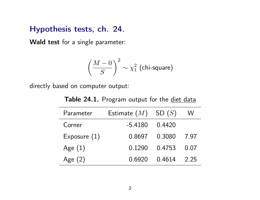
Hypothesis tests, ch. 24.Wald test for a single parameter:

(M − 0

S

)2

∼ χ21 (chi-square)

directly based on computer output:

Table 24.1. Program output for the diet data

Parameter Estimate (M) SD (S) W

Corner -5.4180 0.4420

Exposure (1) 0.8697 0.3080 7.97

Age (1) 0.1290 0.4753 0.07

Age (2) 0.6920 0.4614 2.25

2

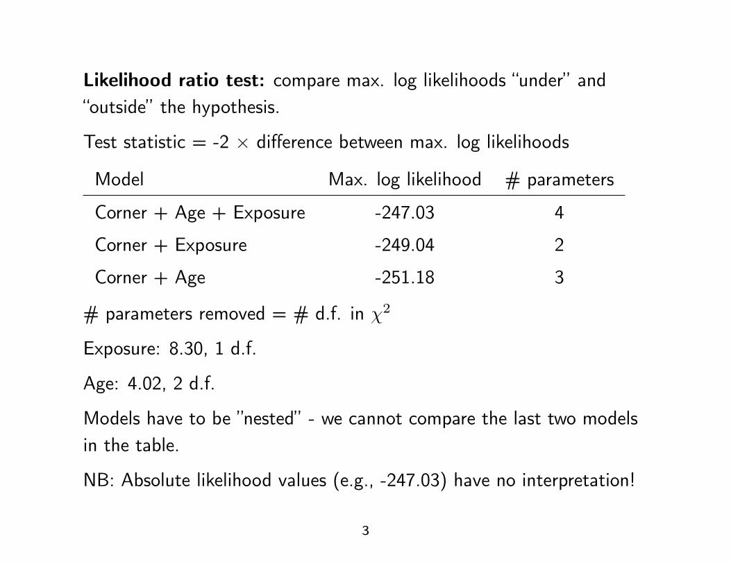
Likelihood ratio test: compare max. log likelihoods “under” and“outside” the hypothesis.

Test statistic = -2 × difference between max. log likelihoods

Model Max. log likelihood # parameters

Corner + Age + Exposure -247.03 4

Corner + Exposure -249.04 2

Corner + Age -251.18 3

# parameters removed = # d.f. in χ2

Exposure: 8.30, 1 d.f.

Age: 4.02, 2 d.f.

Models have to be ”nested” - we cannot compare the last two modelsin the table.

NB: Absolute likelihood values (e.g., -247.03) have no interpretation!

3

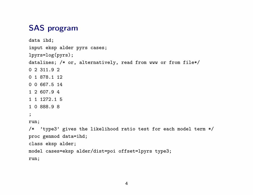
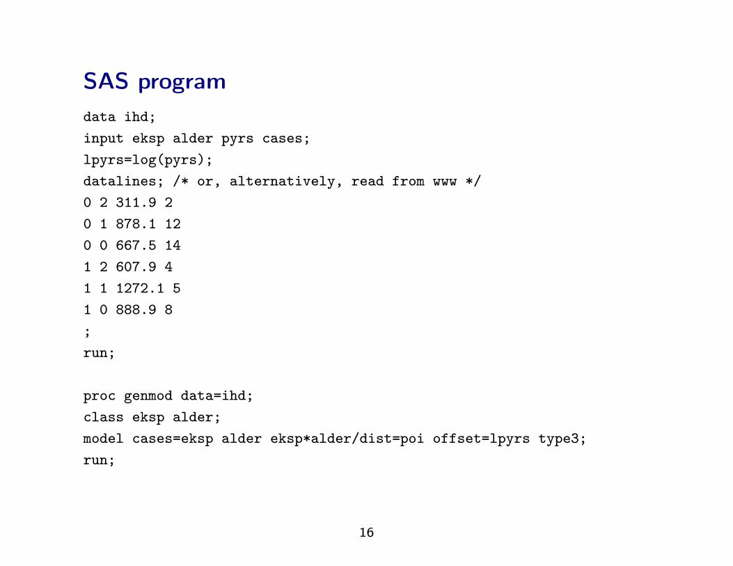
SAS programdata ihd;

input eksp alder pyrs cases;

lpyrs=log(pyrs);

datalines; /* or, alternatively, read from www or from file*/

0 2 311.9 2

0 1 878.1 12

0 0 667.5 14

1 2 607.9 4

1 1 1272.1 5

1 0 888.9 8

;

run;

/* ’type3’ gives the likelihood ratio test for each model term */

proc genmod data=ihd;

class eksp alder;

model cases=eksp alder/dist=poi offset=lpyrs type3;

run;

4

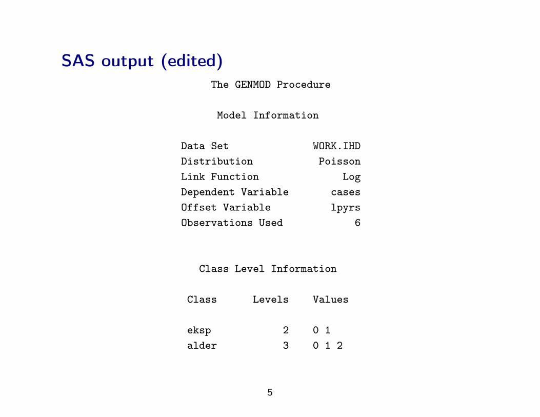
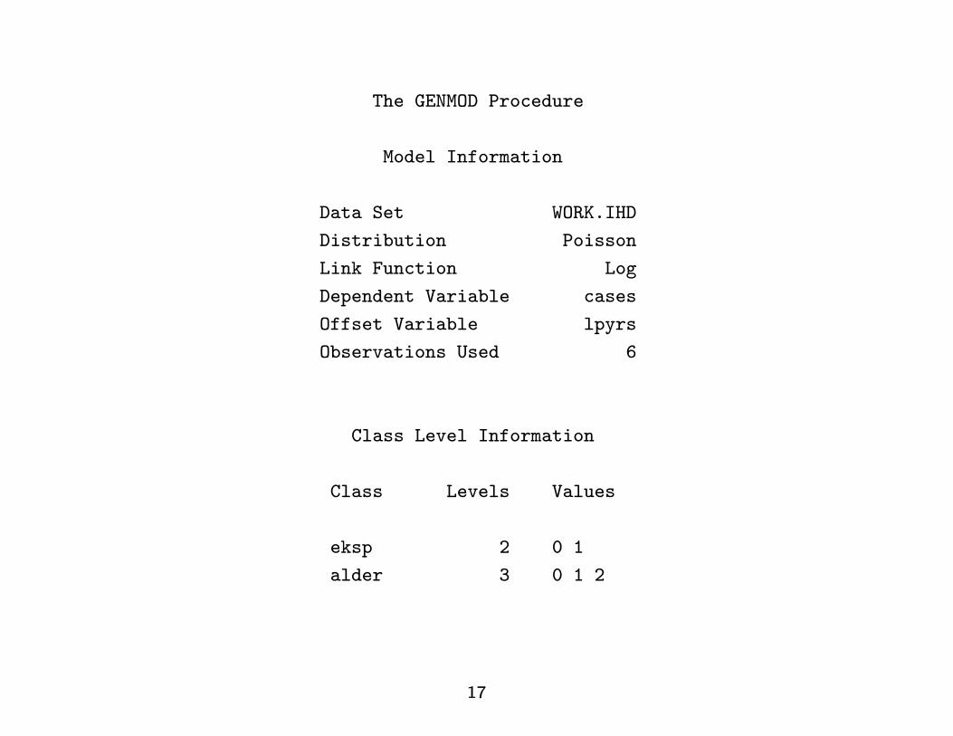
SAS output (edited)The GENMOD Procedure

Model Information

Data Set WORK.IHD

Distribution Poisson

Link Function Log

Dependent Variable cases

Offset Variable lpyrs

Observations Used 6

Class Level Information

Class Levels Values

eksp 2 0 1

alder 3 0 1 2

5

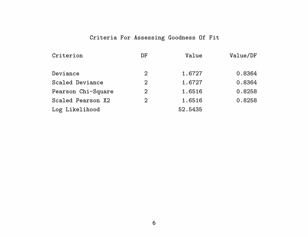
Criteria For Assessing Goodness Of Fit

Criterion DF Value Value/DF

Deviance 2 1.6727 0.8364

Scaled Deviance 2 1.6727 0.8364

Pearson Chi-Square 2 1.6516 0.8258

Scaled Pearson X2 2 1.6516 0.8258

Log Likelihood 52.5435

6

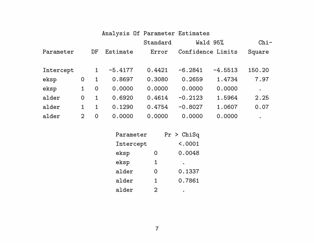
Analysis Of Parameter Estimates

Standard Wald 95% Chi-

Parameter DF Estimate Error Confidence Limits Square

Intercept 1 -5.4177 0.4421 -6.2841 -4.5513 150.20

eksp 0 1 0.8697 0.3080 0.2659 1.4734 7.97

eksp 1 0 0.0000 0.0000 0.0000 0.0000 .

alder 0 1 0.6920 0.4614 -0.2123 1.5964 2.25

alder 1 1 0.1290 0.4754 -0.8027 1.0607 0.07

alder 2 0 0.0000 0.0000 0.0000 0.0000 .

Parameter Pr > ChiSq

Intercept <.0001

eksp 0 0.0048

eksp 1 .

alder 0 0.1337

alder 1 0.7861

alder 2 .

7

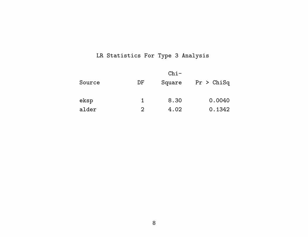
LR Statistics For Type 3 Analysis

Chi-

Source DF Square Pr > ChiSq

eksp 1 8.30 0.0040

alder 2 4.02 0.1342

8

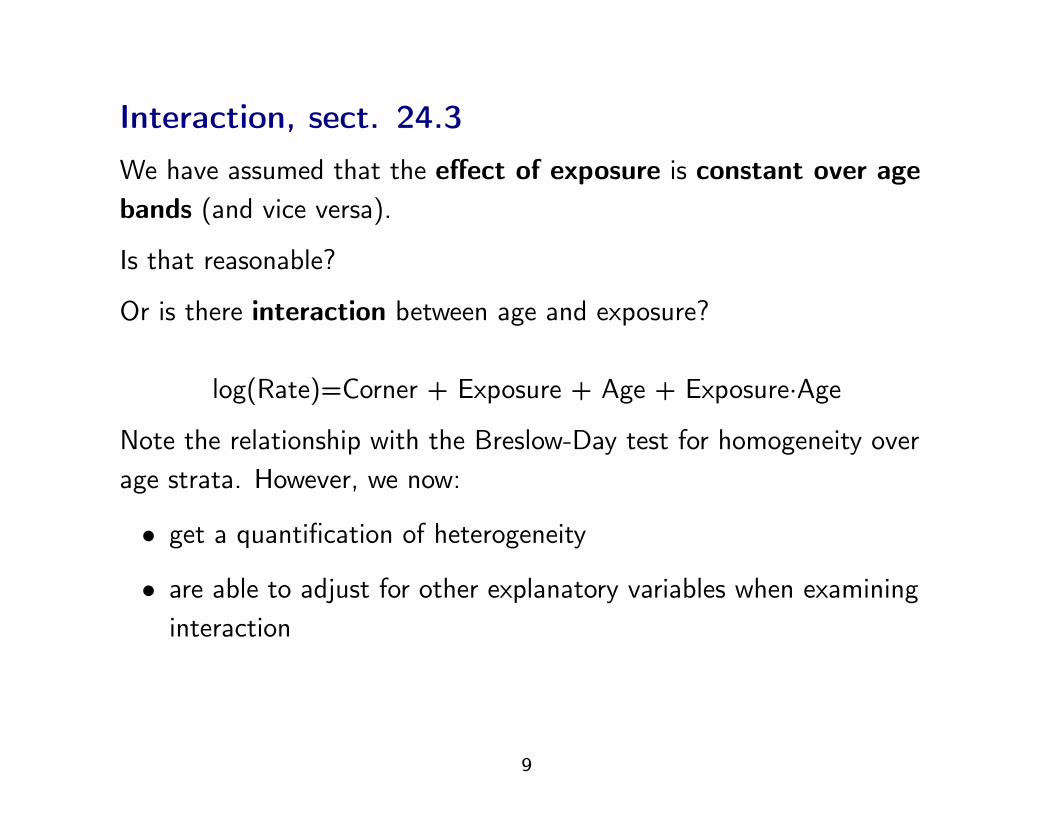
Interaction, sect. 24.3We have assumed that the effect of exposure is constant over agebands (and vice versa).

Is that reasonable?

Or is there interaction between age and exposure?

log(Rate)=Corner + Exposure + Age + Exposure·Age

Note the relationship with the Breslow-Day test for homogeneity overage strata. However, we now:

• get a quantification of heterogeneity

• are able to adjust for other explanatory variables when examininginteraction

9

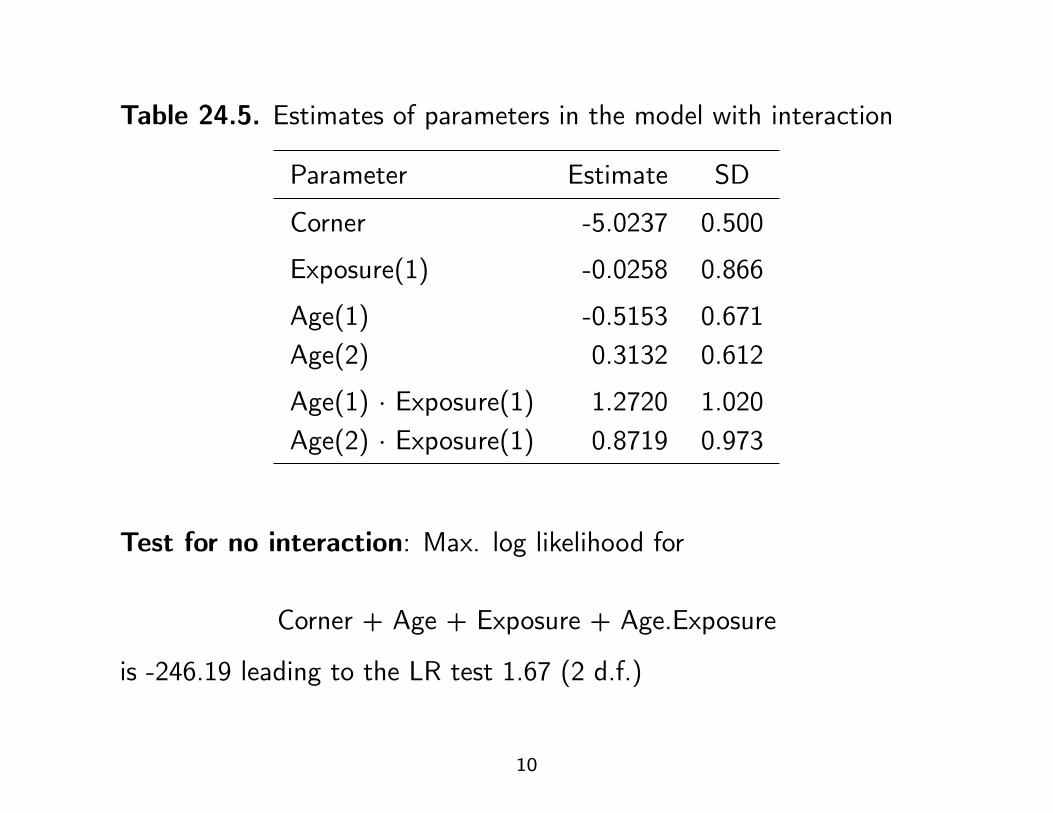
Table 24.5. Estimates of parameters in the model with interaction

Parameter Estimate SD

Corner -5.0237 0.500

Exposure(1) -0.0258 0.866

Age(1) -0.5153 0.671Age(2) 0.3132 0.612

Age(1) · Exposure(1) 1.2720 1.020Age(2) · Exposure(1) 0.8719 0.973

Test for no interaction: Max. log likelihood for

Corner + Age + Exposure + Age.Exposure

is -246.19 leading to the LR test 1.67 (2 d.f.)

10

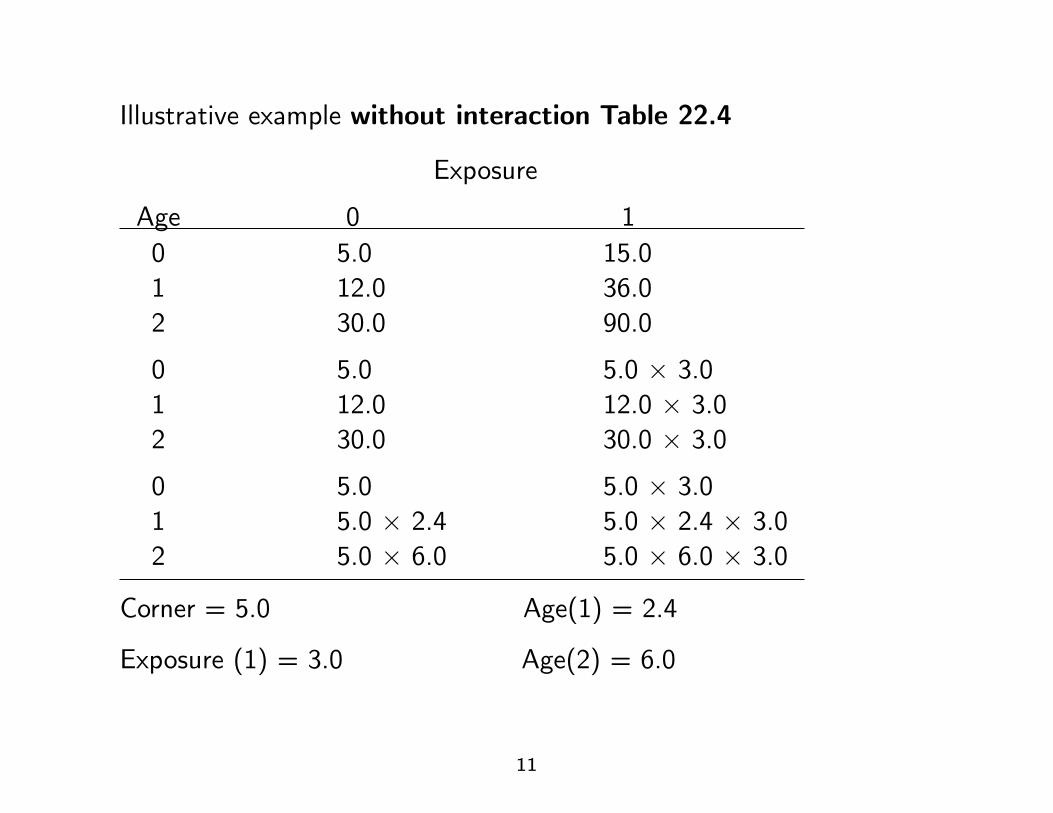
Illustrative example without interaction Table 22.4

Exposure

Age 0 10 5.0 15.01 12.0 36.02 30.0 90.0

0 5.0 5.0 × 3.01 12.0 12.0 × 3.02 30.0 30.0 × 3.0

0 5.0 5.0 × 3.01 5.0 × 2.4 5.0 × 2.4 × 3.02 5.0 × 6.0 5.0 × 6.0 × 3.0

Corner = 5.0 Age(1) = 2.4

Exposure (1) = 3.0 Age(2) = 6.0

11

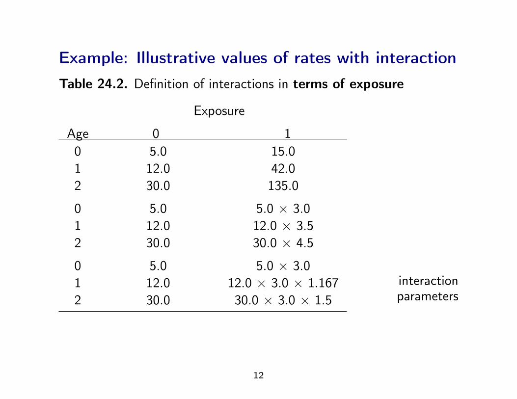
Example: Illustrative values of rates with interactionTable 24.2. Definition of interactions in terms of exposure

Exposure

Age 0 10 5.0 15.01 12.0 42.02 30.0 135.0

0 5.0 5.0 × 3.01 12.0 12.0 × 3.52 30.0 30.0 × 4.5

0 5.0 5.0 × 3.01 12.0 12.0 × 3.0 × 1.1672 30.0 30.0 × 3.0 × 1.5

interactionparameters

12

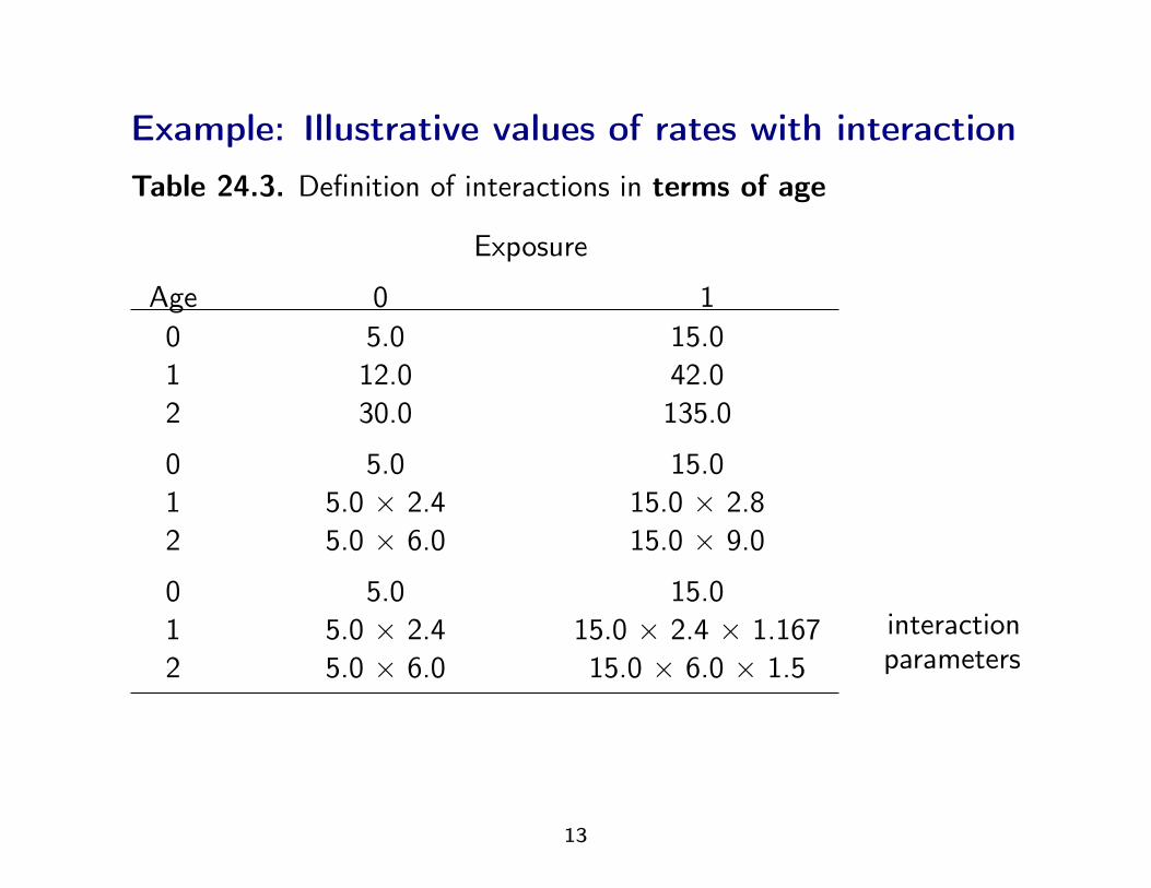
Example: Illustrative values of rates with interactionTable 24.3. Definition of interactions in terms of age

Exposure

Age 0 10 5.0 15.01 12.0 42.02 30.0 135.0

0 5.0 15.01 5.0 × 2.4 15.0 × 2.82 5.0 × 6.0 15.0 × 9.0

0 5.0 15.01 5.0 × 2.4 15.0 × 2.4 × 1.1672 5.0 × 6.0 15.0 × 6.0 × 1.5

interactionparameters

13

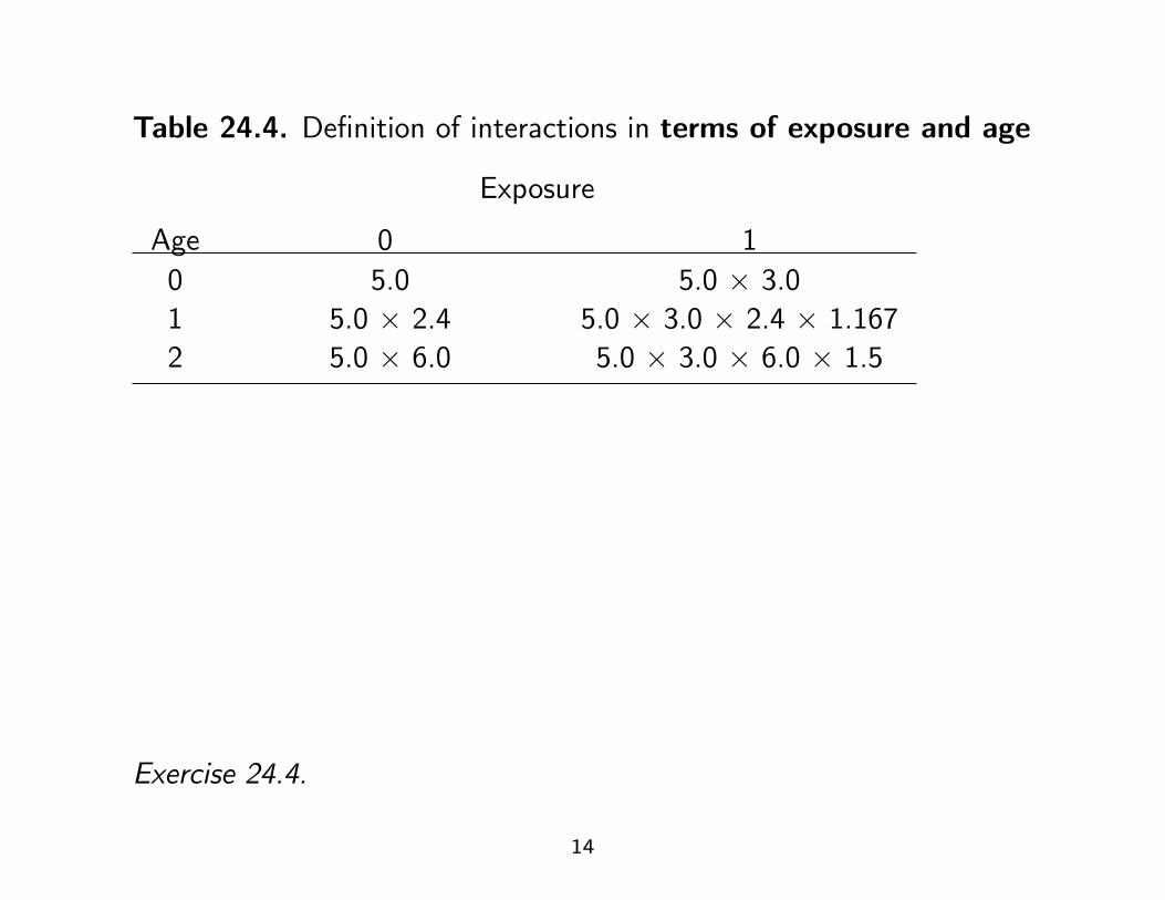
Table 24.4. Definition of interactions in terms of exposure and age

Exposure

Age 0 10 5.0 5.0 × 3.01 5.0 × 2.4 5.0 × 3.0 × 2.4 × 1.1672 5.0 × 6.0 5.0 × 3.0 × 6.0 × 1.5

Exercise 24.4.

14

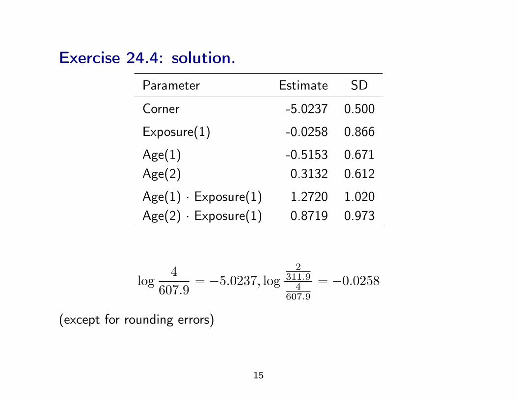
Exercise 24.4: solution.


Corner -5.0237 0.500

Exposure(1) -0.0258 0.866

Age(1) -0.5153 0.671Age(2) 0.3132 0.612

Age(1) · Exposure(1) 1.2720 1.020Age(2) · Exposure(1) 0.8719 0.973

log4

607.9= −5.0237, log

2311.9

4607.9

= −0.0258

(except for rounding errors)

15

SAS programdata ihd;

input eksp alder pyrs cases;

lpyrs=log(pyrs);

datalines; /* or, alternatively, read from www */

0 2 311.9 2

0 1 878.1 12

0 0 667.5 14

1 2 607.9 4

1 1 1272.1 5

1 0 888.9 8

;

run;

proc genmod data=ihd;

class eksp alder;

model cases=eksp alder eksp*alder/dist=poi offset=lpyrs type3;

run;

16

The GENMOD Procedure

Model Information

Data Set WORK.IHD

Distribution Poisson

Link Function Log

Dependent Variable cases

Offset Variable lpyrs

Observations Used 6

Class Level Information

Class Levels Values

eksp 2 0 1

alder 3 0 1 2

17

Criteria For Assessing Goodness Of Fit

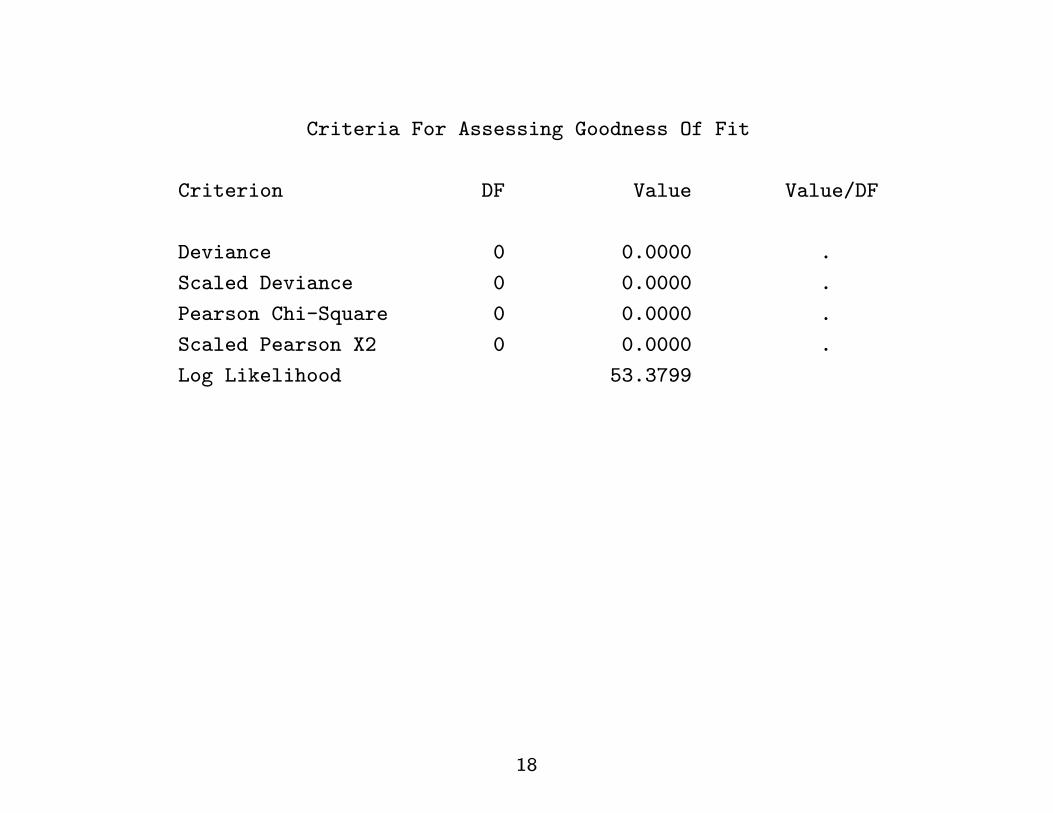
Criterion DF Value Value/DF

Deviance 0 0.0000 .

Scaled Deviance 0 0.0000 .

Pearson Chi-Square 0 0.0000 .

Scaled Pearson X2 0 0.0000 .

Log Likelihood 53.3799

18

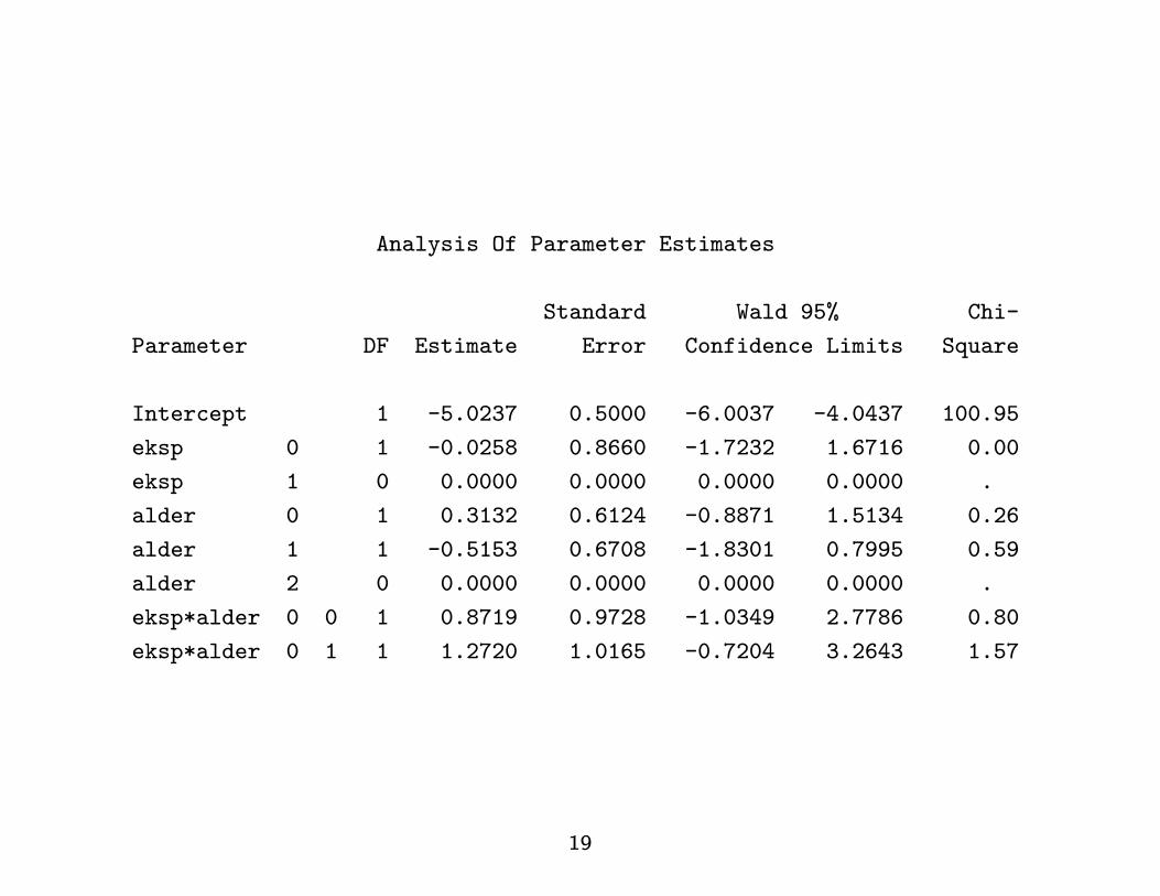
Analysis Of Parameter Estimates

Standard Wald 95% Chi-

Parameter DF Estimate Error Confidence Limits Square

Intercept 1 -5.0237 0.5000 -6.0037 -4.0437 100.95

eksp 0 1 -0.0258 0.8660 -1.7232 1.6716 0.00

eksp 1 0 0.0000 0.0000 0.0000 0.0000 .

alder 0 1 0.3132 0.6124 -0.8871 1.5134 0.26

alder 1 1 -0.5153 0.6708 -1.8301 0.7995 0.59

alder 2 0 0.0000 0.0000 0.0000 0.0000 .

eksp*alder 0 0 1 0.8719 0.9728 -1.0349 2.7786 0.80

eksp*alder 0 1 1 1.2720 1.0165 -0.7204 3.2643 1.57

19

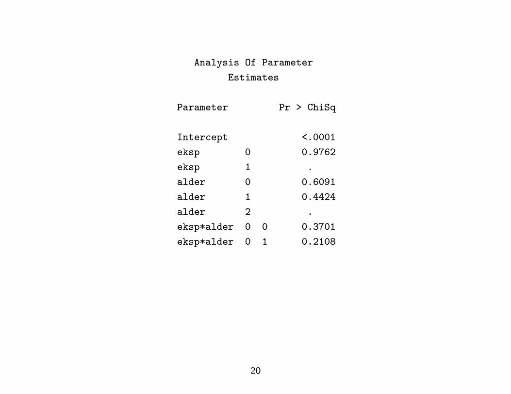
Analysis Of Parameter

Estimates

Parameter Pr > ChiSq

Intercept <.0001

eksp 0 0.9762

eksp 1 .

alder 0 0.6091

alder 1 0.4424

alder 2 .

eksp*alder 0 0 0.3701

eksp*alder 0 1 0.2108

20

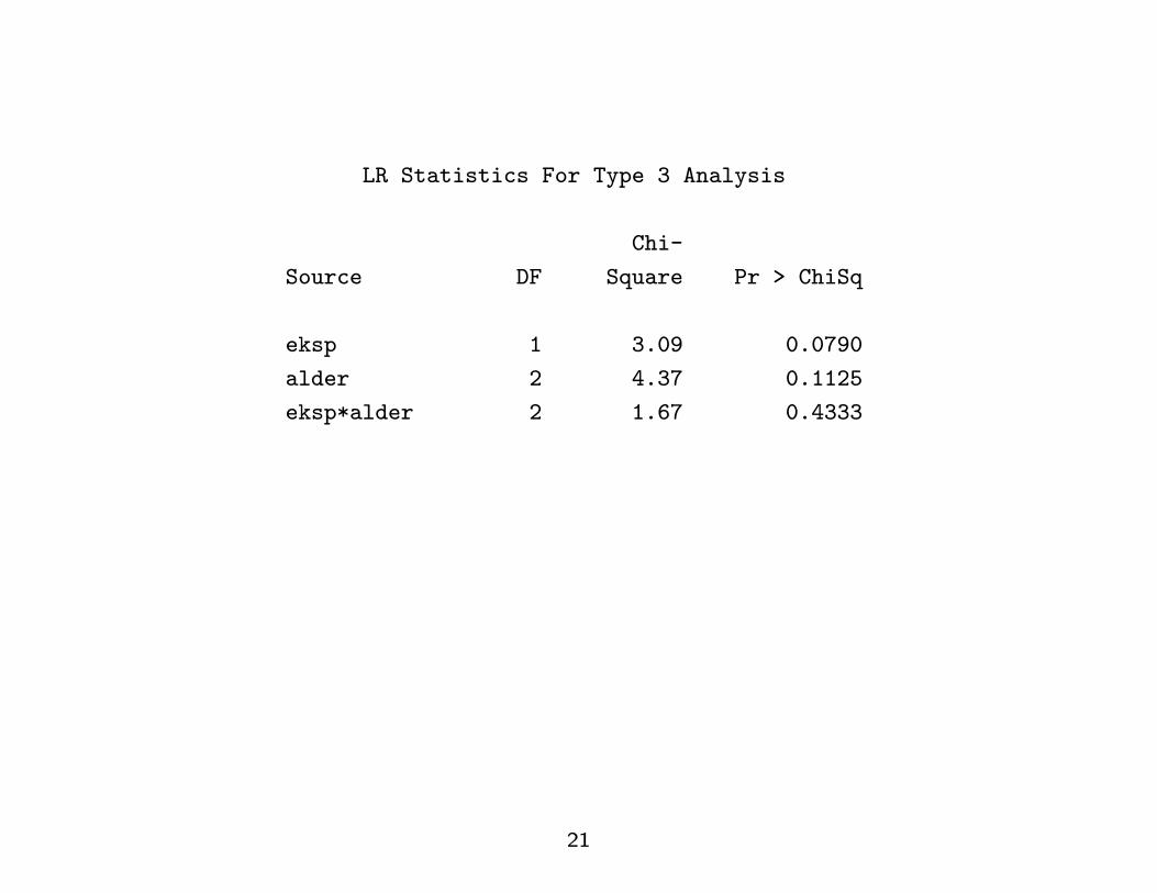
LR Statistics For Type 3 Analysis

Chi-

Source DF Square Pr > ChiSq

eksp 1 3.09 0.0790

alder 2 4.37 0.1125

eksp*alder 2 1.67 0.4333

21

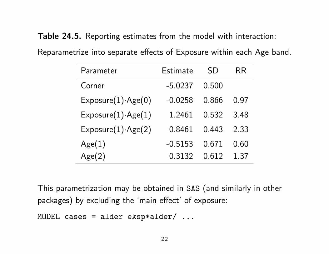
Table 24.5. Reporting estimates from the model with interaction:

Reparametrize into separate effects of Exposure within each Age band.

Parameter Estimate SD RR

Corner -5.0237 0.500

Exposure(1)·Age(0) -0.0258 0.866 0.97

Exposure(1)·Age(1) 1.2461 0.532 3.48

Exposure(1)·Age(2) 0.8461 0.443 2.33

Age(1) -0.5153 0.671 0.60Age(2) 0.3132 0.612 1.37

This parametrization may be obtained in SAS (and similarly in otherpackages) by excluding the ‘main effect’ of exposure:

MODEL cases = alder eksp*alder/ ...

22

Interactions: which to study?When the model contains p covariates there are p(p− 1)/2 possibletwo-factor interactions (e.g., 45 for p = 10).

It is out of the question to study them all, so a generalrecommendation is to restrict attention to those that werepre-specified in the research protocol:

“Don’t ask a question if you are not interested in the reply!”

There will also be a type I error problem: “if you ask too manyquestions you will get too many wrong answers”.

23

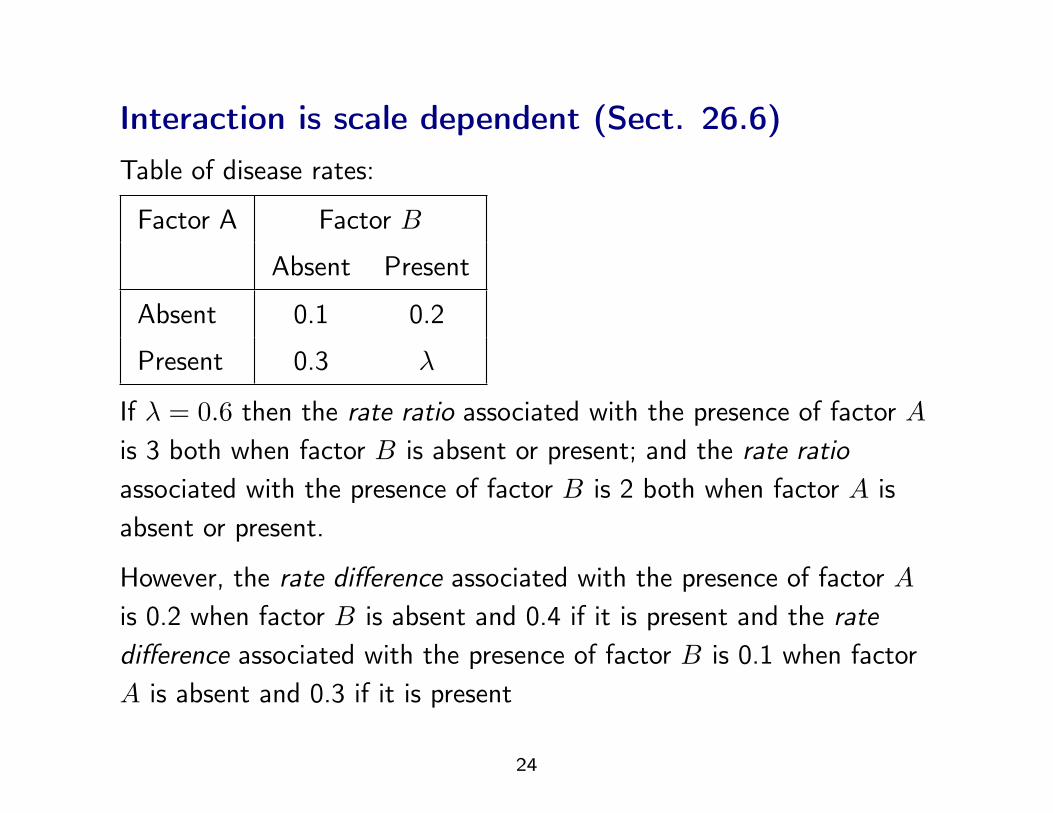
Interaction is scale dependent (Sect. 26.6)Table of disease rates:

Factor A Factor B

Absent Present

Absent 0.1 0.2

Present 0.3 λ

If λ = 0.6 then the rate ratio associated with the presence of factor Ais 3 both when factor B is absent or present; and the rate ratioassociated with the presence of factor B is 2 both when factor A isabsent or present.

However, the rate difference associated with the presence of factor Ais 0.2 when factor B is absent and 0.4 if it is present and the ratedifference associated with the presence of factor B is 0.1 when factorA is absent and 0.3 if it is present

24

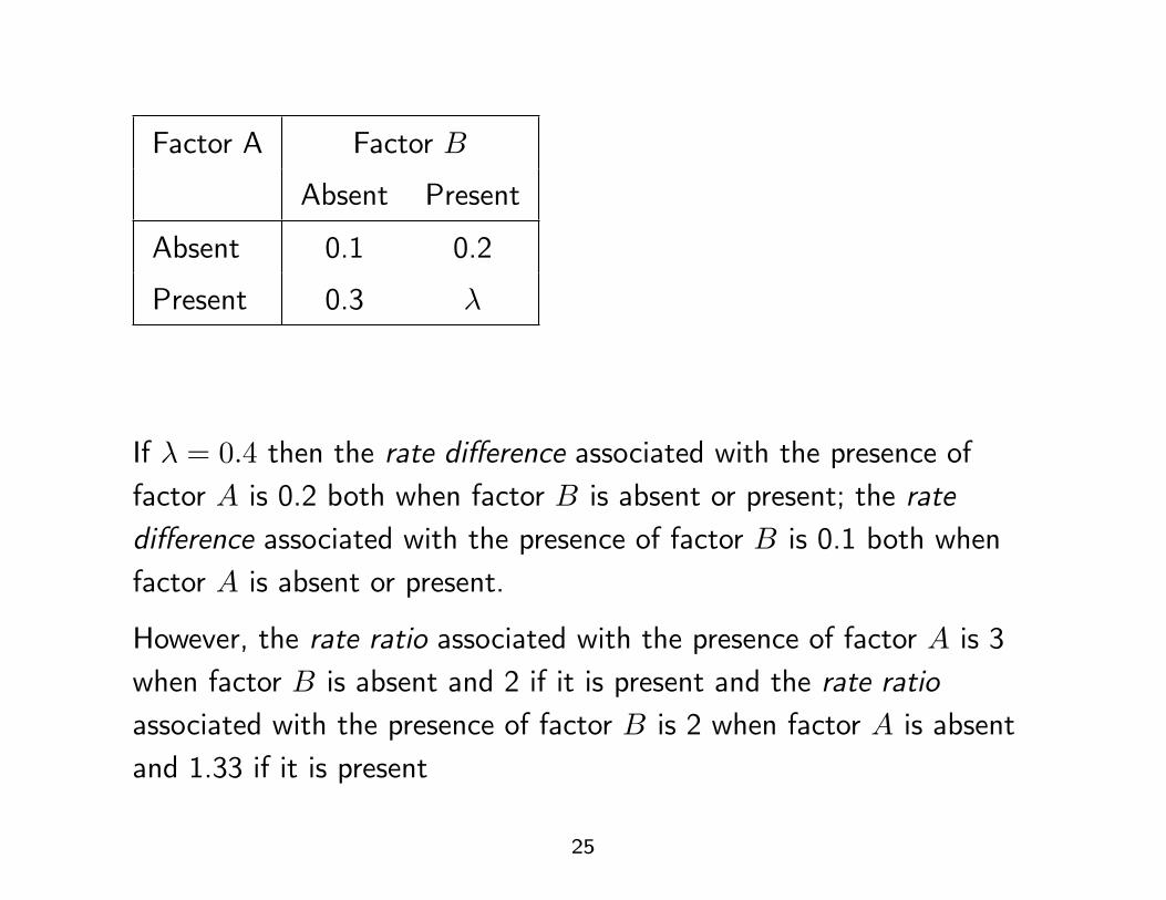
Factor A Factor B

Absent Present

Absent 0.1 0.2

Present 0.3 λ

If λ = 0.4 then the rate difference associated with the presence offactor A is 0.2 both when factor B is absent or present; the ratedifference associated with the presence of factor B is 0.1 both whenfactor A is absent or present.

However, the rate ratio associated with the presence of factor A is 3when factor B is absent and 2 if it is present and the rate ratioassociated with the presence of factor B is 2 when factor A is absentand 1.33 if it is present

25

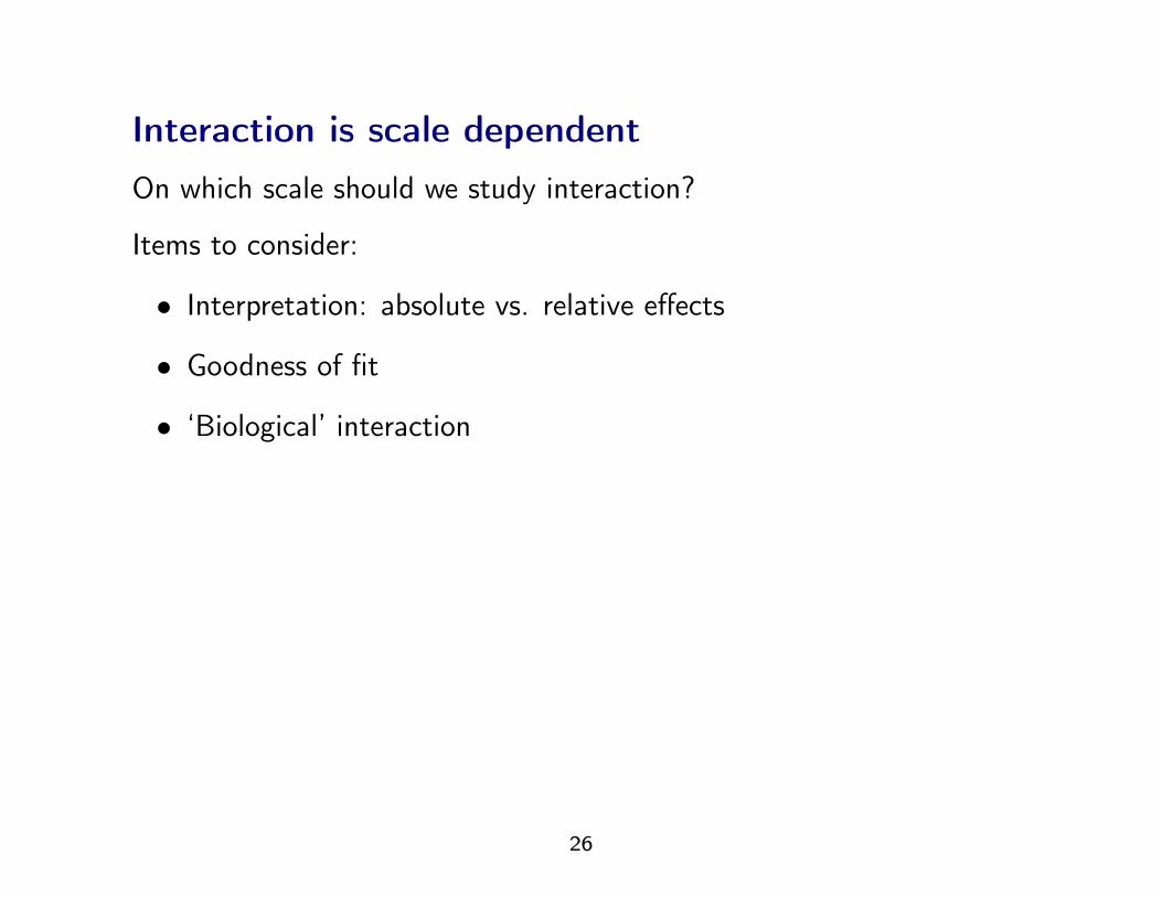
Interaction is scale dependentOn which scale should we study interaction?

Items to consider:

• Interpretation: absolute vs. relative effects

• Goodness of fit

• ‘Biological’ interaction

26

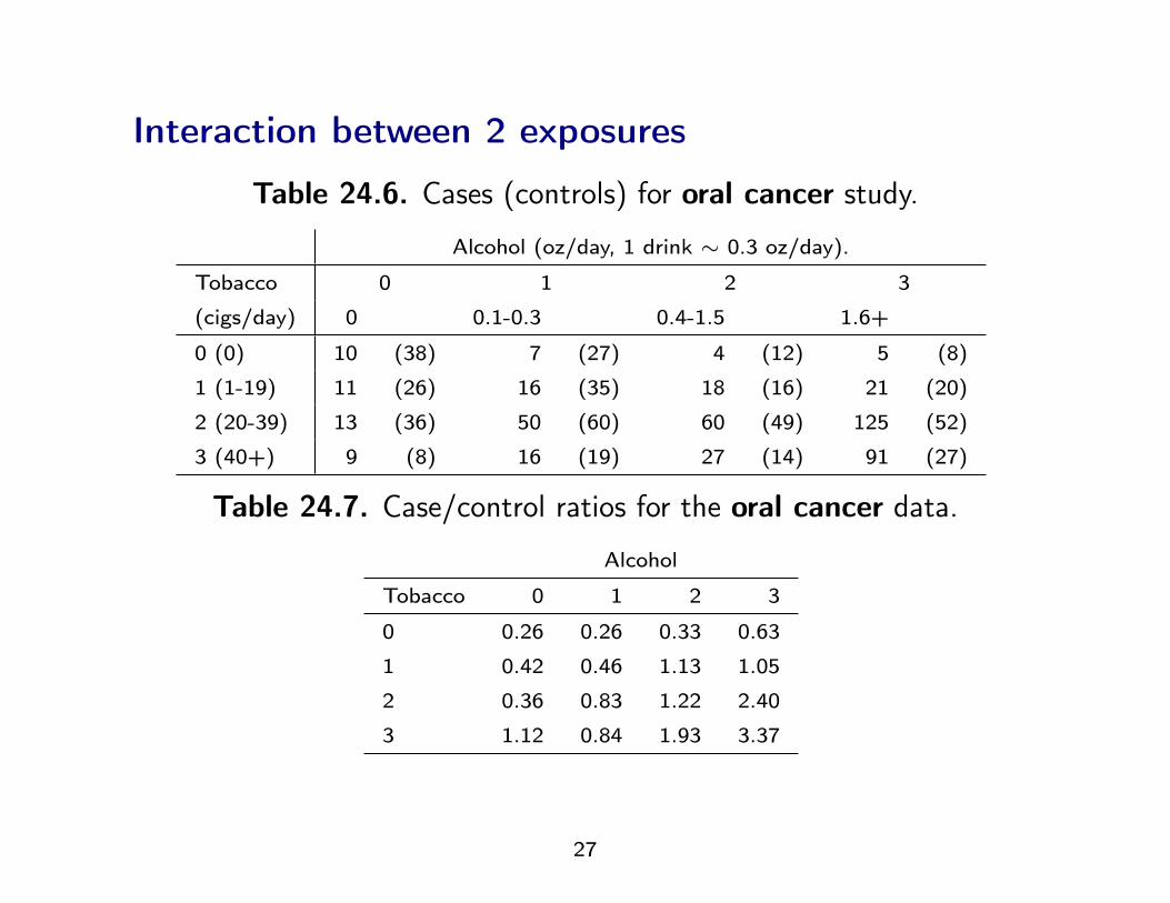
Interaction between 2 exposures

Table 24.6. Cases (controls) for oral cancer study.

Alcohol (oz/day, 1 drink ∼ 0.3 oz/day).

Tobacco 0 1 2 3

(cigs/day) 0 0.1-0.3 0.4-1.5 1.6+

0 (0) 10 (38) 7 (27) 4 (12) 5 (8)

1 (1-19) 11 (26) 16 (35) 18 (16) 21 (20)

2 (20-39) 13 (36) 50 (60) 60 (49) 125 (52)

3 (40+) 9 (8) 16 (19) 27 (14) 91 (27)

Table 24.7. Case/control ratios for the oral cancer data.

Alcohol

Tobacco 0 1 2 3

0 0.26 0.26 0.33 0.63

1 0.42 0.46 1.13 1.05

2 0.36 0.83 1.22 2.40

3 1.12 0.84 1.93 3.37

27

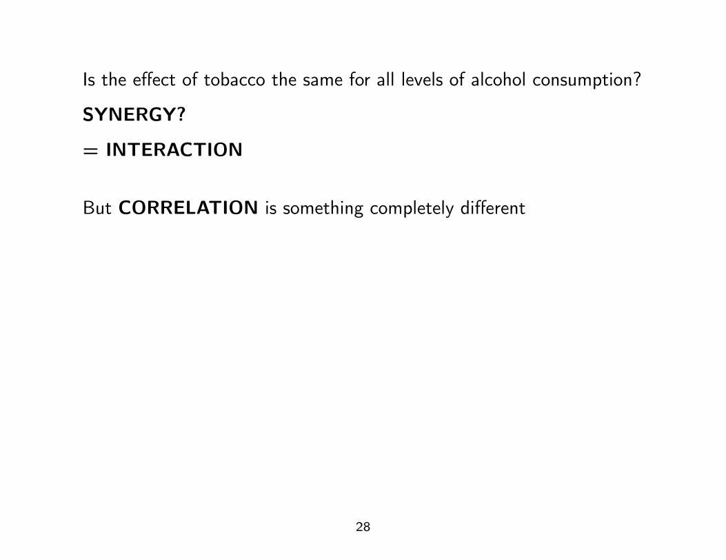
Is the effect of tobacco the same for all levels of alcohol consumption?

SYNERGY?

= INTERACTION

But CORRELATION is something completely different

28

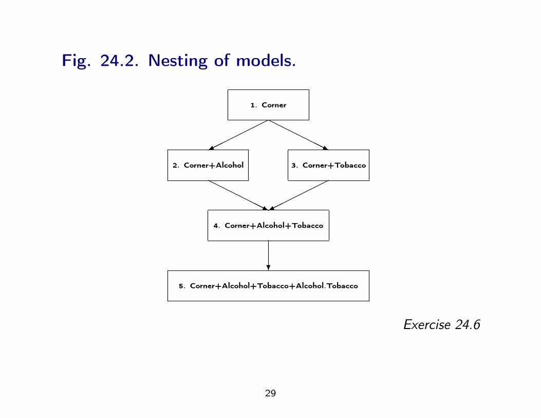
Fig. 24.2. Nesting of models.

5. Corner+Alcohol+Tobacco+Alcohol.Tobacco

4. Corner+Alcohol+Tobacco

2. Corner+Alcohol 3. Corner+Tobacco

1. Corner

HHHHHj

HHHHHj

��

��

?

Exercise 24.6

29

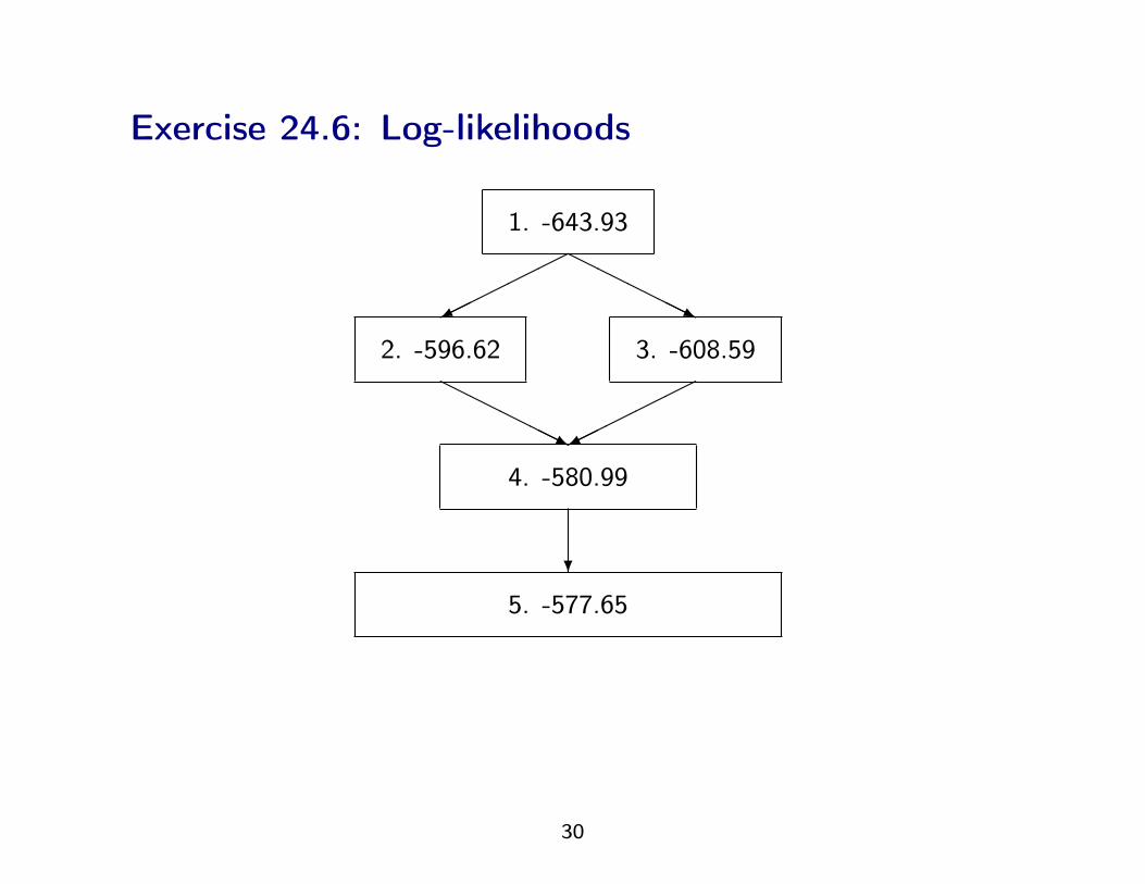
Exercise 24.6: Log-likelihoods

5. -577.65

4. -580.99

2. -596.62 3. -608.59

1. -643.93

HHHHHj

HHHHHj

��

��

?

30

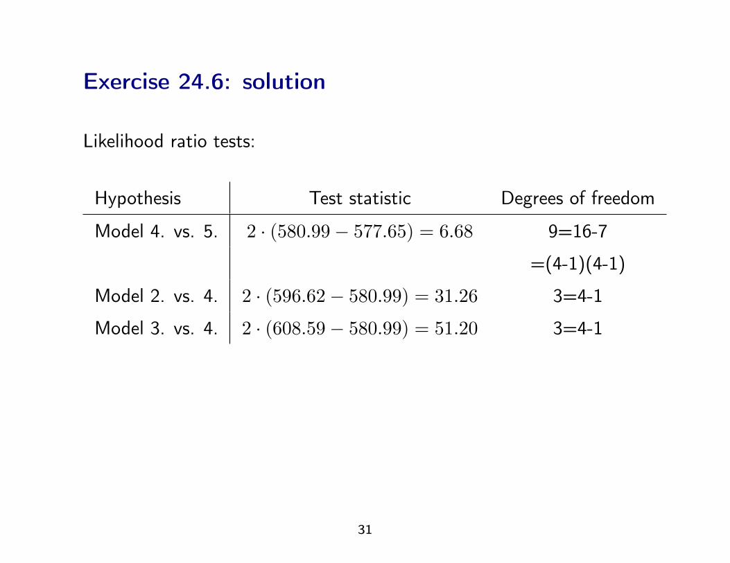
Exercise 24.6: solution

Likelihood ratio tests:

Hypothesis Test statistic Degrees of freedom

Model 4. vs. 5. 2 · (580.99− 577.65) = 6.68 9=16-7

=(4-1)(4-1)

Model 2. vs. 4. 2 · (596.62− 580.99) = 31.26 3=4-1

Model 3. vs. 4. 2 · (608.59− 580.99) = 51.20 3=4-1

31

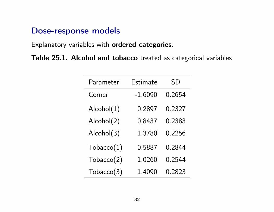
Dose-response modelsExplanatory variables with ordered categories.

Table 25.1. Alcohol and tobacco treated as categorical variables


Corner -1.6090 0.2654

Alcohol(1) 0.2897 0.2327

Alcohol(2) 0.8437 0.2383

Alcohol(3) 1.3780 0.2256

Tobacco(1) 0.5887 0.2844

Tobacco(2) 1.0260 0.2544

Tobacco(3) 1.4090 0.2823

32

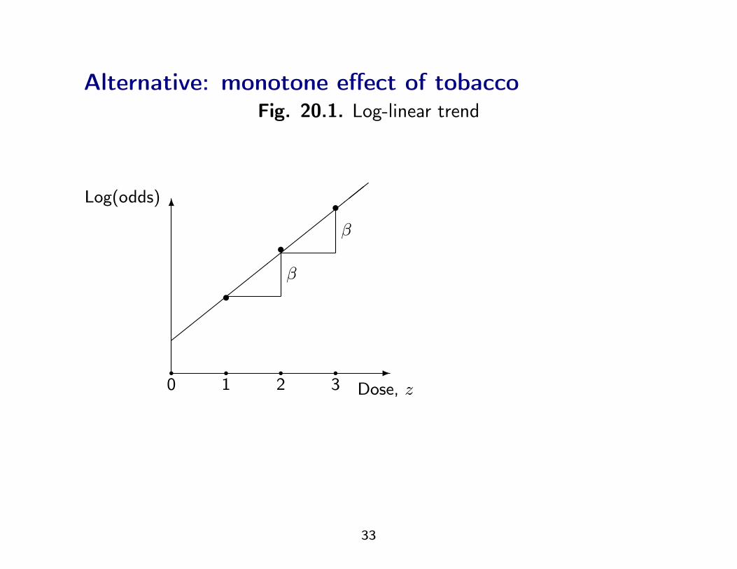
Alternative: monotone effect of tobaccoFig. 20.1. Log-linear trend

-

6Log(odds)

q q q q0 1 2 3 Dose, z

rr

r

###########

β

β

33

Look at successive differences between effects:

Tobacco(1), Tobacco(2)-Tobacco(1), Tobacco(3)-Tobacco(2)

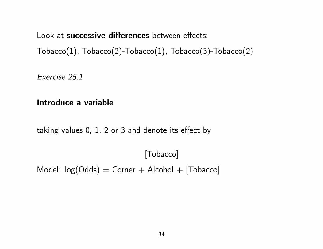
Exercise 25.1

Introduce a variable

taking values 0, 1, 2 or 3 and denote its effect by

[Tobacco]

Model: log(Odds) = Corner + Alcohol + [Tobacco]

34

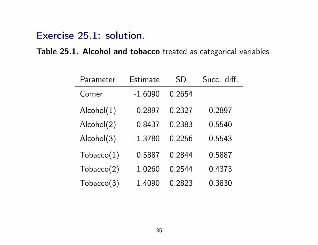
Exercise 25.1: solution.Table 25.1. Alcohol and tobacco treated as categorical variables

Parameter Estimate SD Succ. diff.

Corner -1.6090 0.2654

Alcohol(1) 0.2897 0.2327 0.2897

Alcohol(2) 0.8437 0.2383 0.5540

Alcohol(3) 1.3780 0.2256 0.5543

Tobacco(1) 0.5887 0.2844 0.5887

Tobacco(2) 1.0260 0.2544 0.4373

Tobacco(3) 1.4090 0.2823 0.3830

35

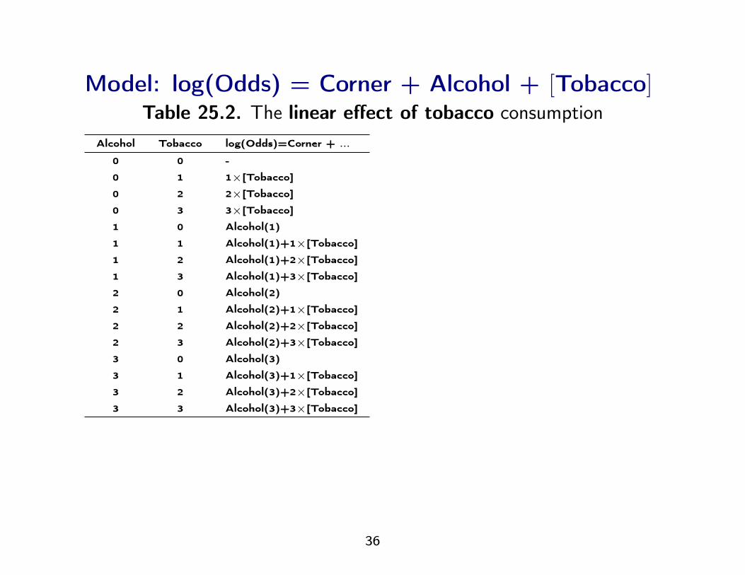
Model: log(Odds) = Corner + Alcohol + [Tobacco]Table 25.2. The linear effect of tobacco consumption

Alcohol Tobacco log(Odds)=Corner + ...

0 0 -

0 1 1×[Tobacco]

0 2 2×[Tobacco]

0 3 3×[Tobacco]

1 0 Alcohol(1)

1 1 Alcohol(1)+1×[Tobacco]



2 0 Alcohol(2)




3 0 Alcohol(3)




36

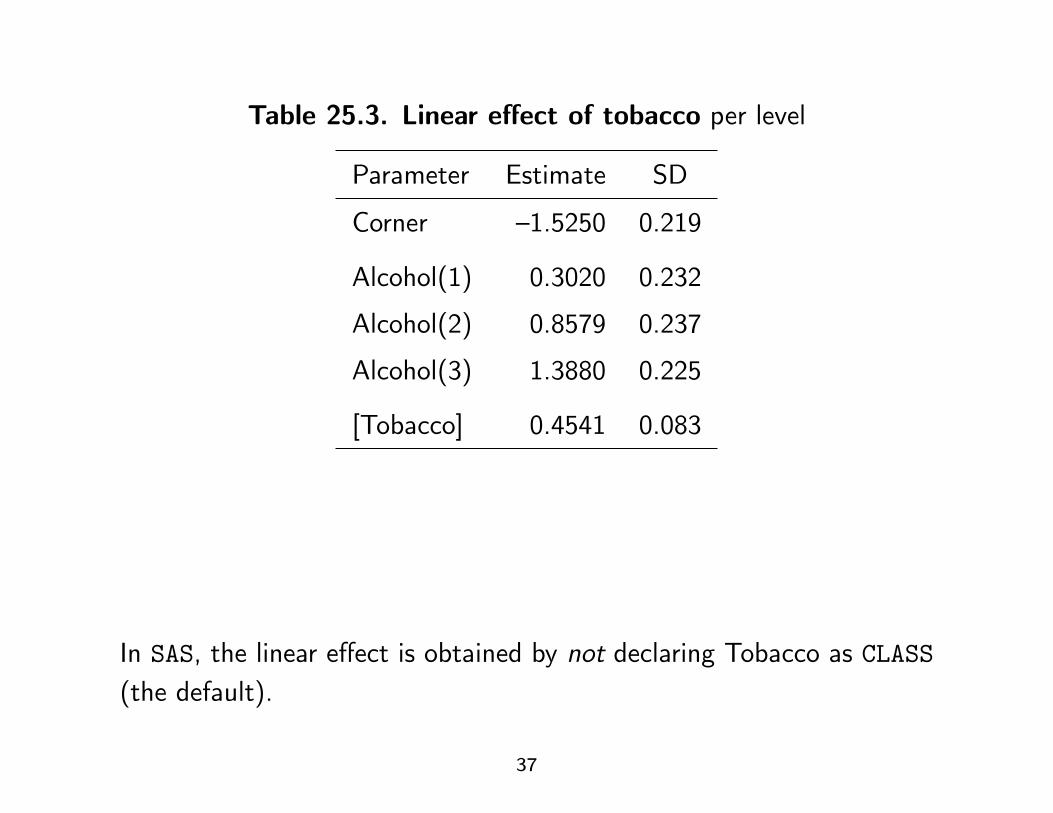
Table 25.3. Linear effect of tobacco per level


Corner –1.5250 0.219

Alcohol(1) 0.3020 0.232

Alcohol(2) 0.8579 0.237

Alcohol(3) 1.3880 0.225

[Tobacco] 0.4541 0.083

In SAS, the linear effect is obtained by not declaring Tobacco as CLASS(the default).

37

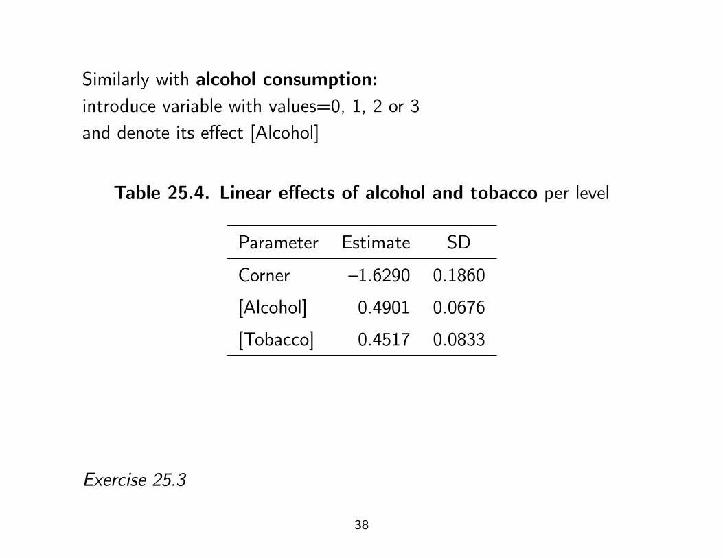
Similarly with alcohol consumption:introduce variable with values=0, 1, 2 or 3and denote its effect [Alcohol]

Table 25.4. Linear effects of alcohol and tobacco per level


Corner –1.6290 0.1860

[Alcohol] 0.4901 0.0676

[Tobacco] 0.4517 0.0833

Exercise 25.3

38

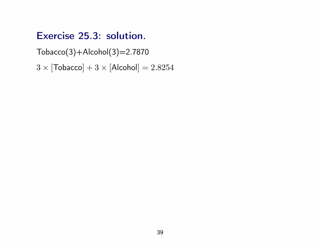
Exercise 25.3: solution.Tobacco(3)+Alcohol(3)=2.7870

3× [Tobacco] + 3× [Alcohol] = 2.8254

39

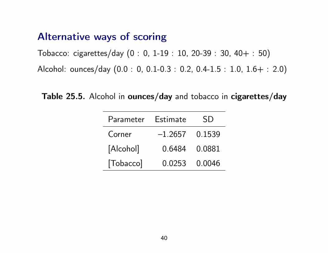
Alternative ways of scoringTobacco: cigarettes/day (0 : 0, 1-19 : 10, 20-39 : 30, 40+ : 50)

Alcohol: ounces/day (0.0 : 0, 0.1-0.3 : 0.2, 0.4-1.5 : 1.0, 1.6+ : 2.0)

Table 25.5. Alcohol in ounces/day and tobacco in cigarettes/day


Corner –1.2657 0.1539

[Alcohol] 0.6484 0.0881

[Tobacco] 0.0253 0.0046

40

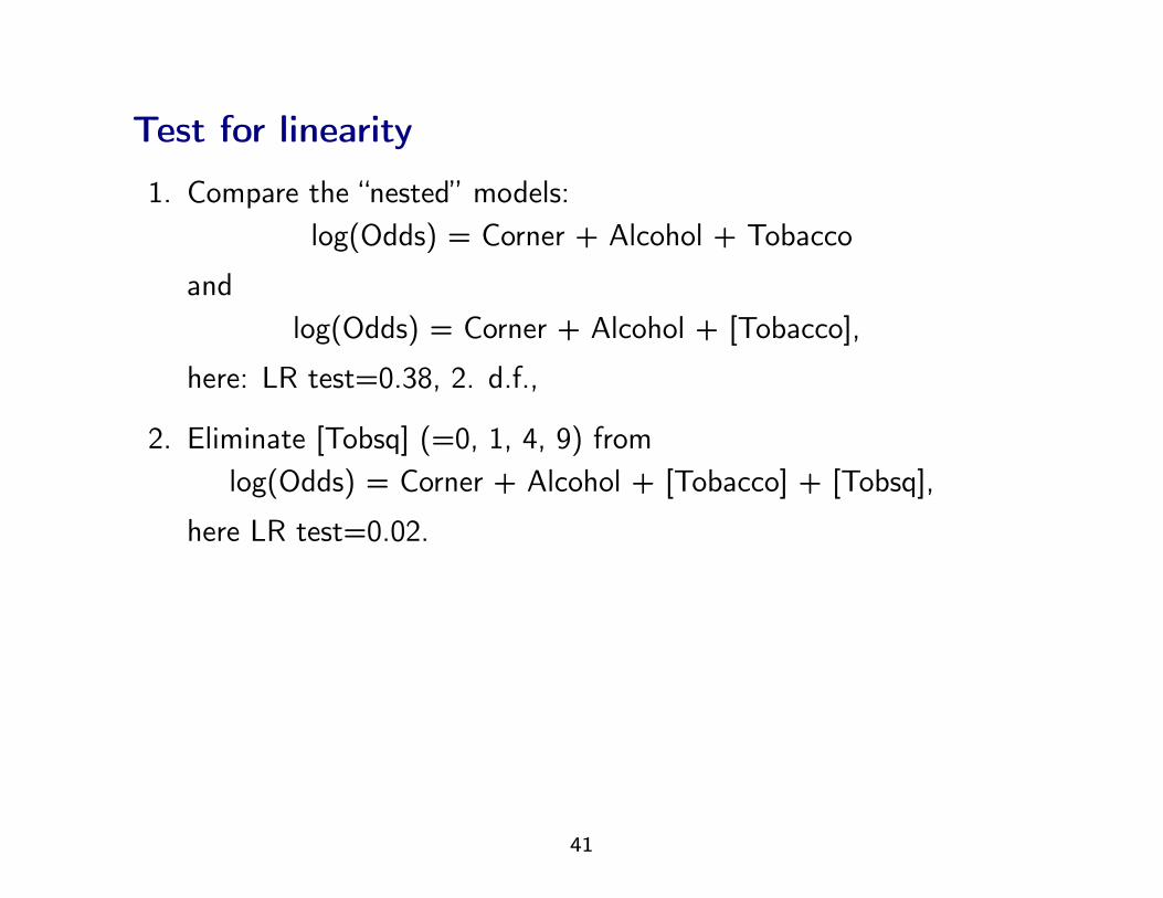
Test for linearity

1. Compare the “nested” models:log(Odds) = Corner + Alcohol + Tobacco

andlog(Odds) = Corner + Alcohol + [Tobacco],

here: LR test=0.38, 2. d.f.,

2. Eliminate [Tobsq] (=0, 1, 4, 9) fromlog(Odds) = Corner + Alcohol + [Tobacco] + [Tobsq],

here LR test=0.02.

41

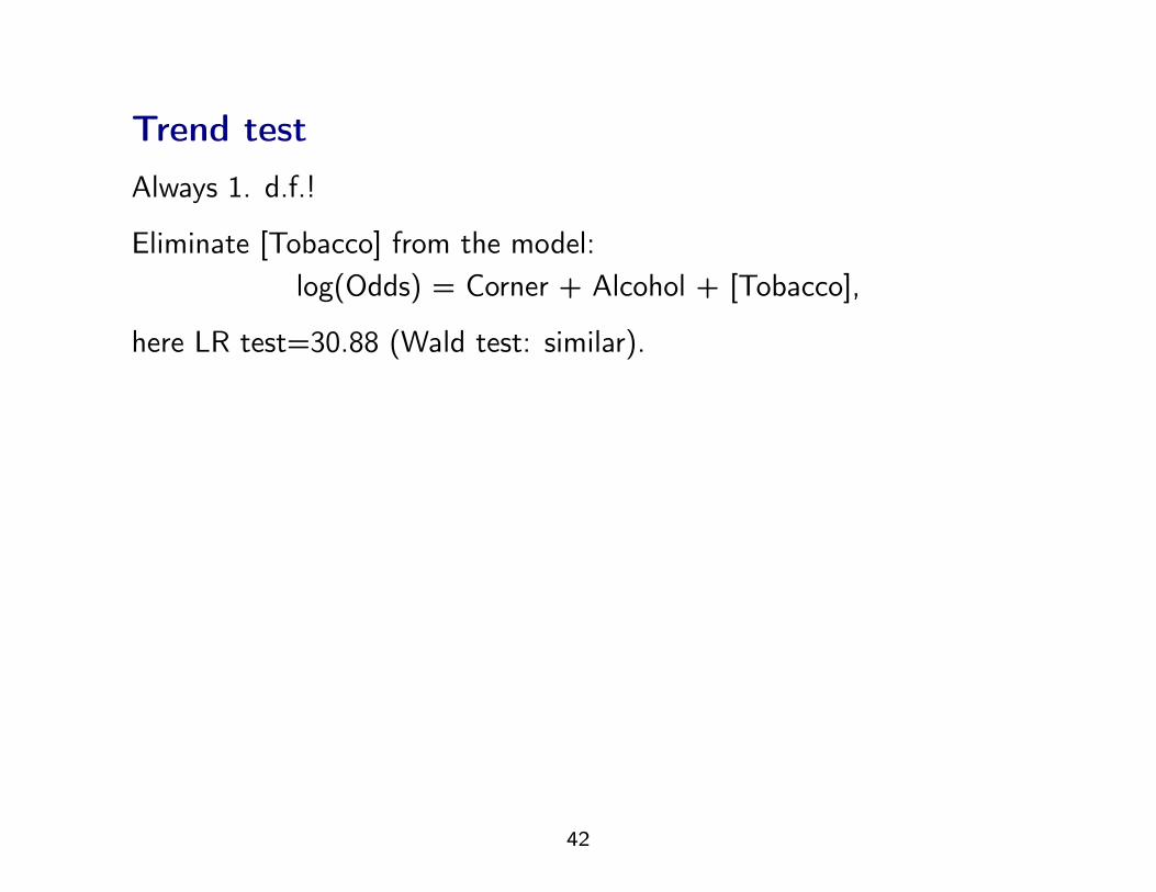
Trend testAlways 1. d.f.!

Eliminate [Tobacco] from the model:log(Odds) = Corner + Alcohol + [Tobacco],

here LR test=30.88 (Wald test: similar).

42

Using individual levels of the quantitative covariateWhy not use individual levels, that is, a truly quantitative covariateand no categorization at all?

Pros and cons

• Information is lost by categorization

• Categories may be more robust (e.g., smoking)

• Few outliers may have large influence (“Casanova effect”!)

• Model with a linear effect is no longer “nested” in categoricalmodel ⇒ alternative alternatives are needed when testing linearity

43

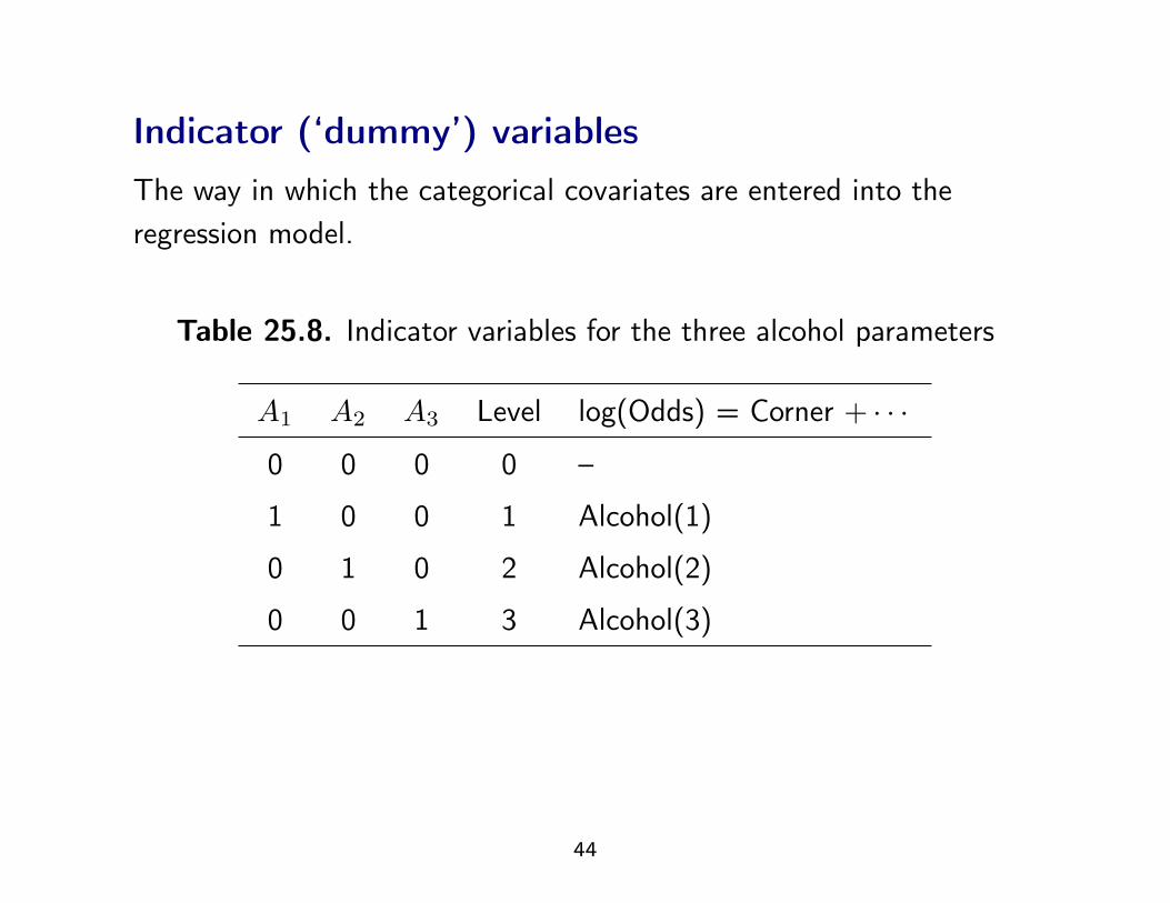
Indicator (‘dummy’) variablesThe way in which the categorical covariates are entered into theregression model.

Table 25.8. Indicator variables for the three alcohol parameters

A1 A2 A3 Level log(Odds) = Corner + · · ·

0 0 0 0 –

1 0 0 1 Alcohol(1)

0 1 0 2 Alcohol(2)

0 0 1 3 Alcohol(3)

44

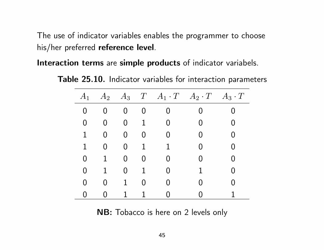
The use of indicator variables enables the programmer to choosehis/her preferred reference level.

Interaction terms are simple products of indicator variabels.

Table 25.10. Indicator variables for interaction parameters

A1 A2 A3 T A1 · T A2 · T A3 · T

0 0 0 0 0 0 00 0 0 1 0 0 01 0 0 0 0 0 01 0 0 1 1 0 00 1 0 0 0 0 00 1 0 1 0 1 00 0 1 0 0 0 00 0 1 1 0 0 1

NB: Tobacco is here on 2 levels only

45

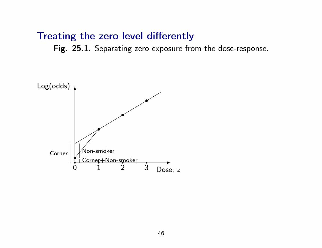
Treating the zero level differentlyFig. 25.1. Separating zero exposure from the dose-response.

-

6Log(odds)

q q q q0 1 2 3 Dose, z

rr r r

CornerCorner+Non-smoker

Non-smoker

""""""""

%%%%"""

46

Corresponds to adding a new variable [Non-smoker]

Table 25.11. Separating zero exposure from the dose-response

Tobacco Non-smoker log(Odds) = Corner + · · ·

0 1 [Non-smoker]

1 0 1 × [Tobacco]

2 0 2 × [Tobacco]

3 0 3 × [Tobacco]

(Alternative: include [Smoker] = 1 - [Non-smoker])

47

Truly quantitative covariates, xIn a model like

log(Rate)=Corner + Exposure + [x]

the effect of x is assumed to be linear, i.e. [x] expresses the change inlog(Rate) per 1 unit change of x.

To test for linearity, one may add [xsq] to the model where xsq= x2.

An alternative alternative is a linear spline.

48

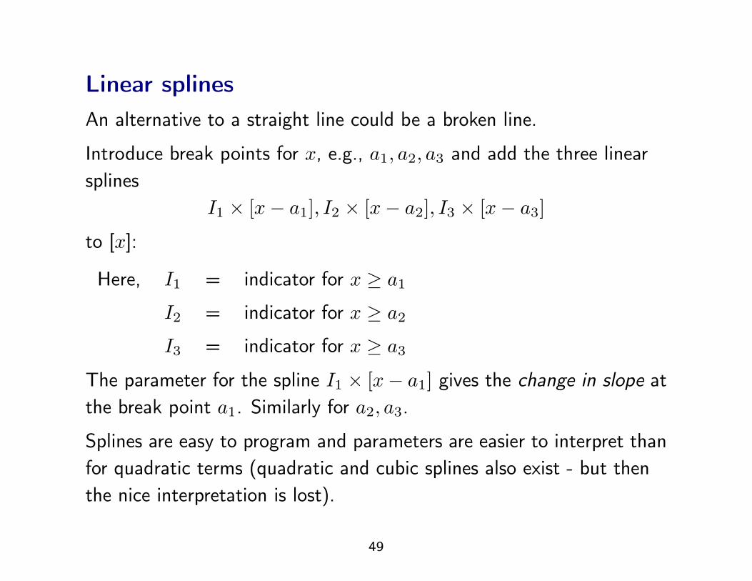
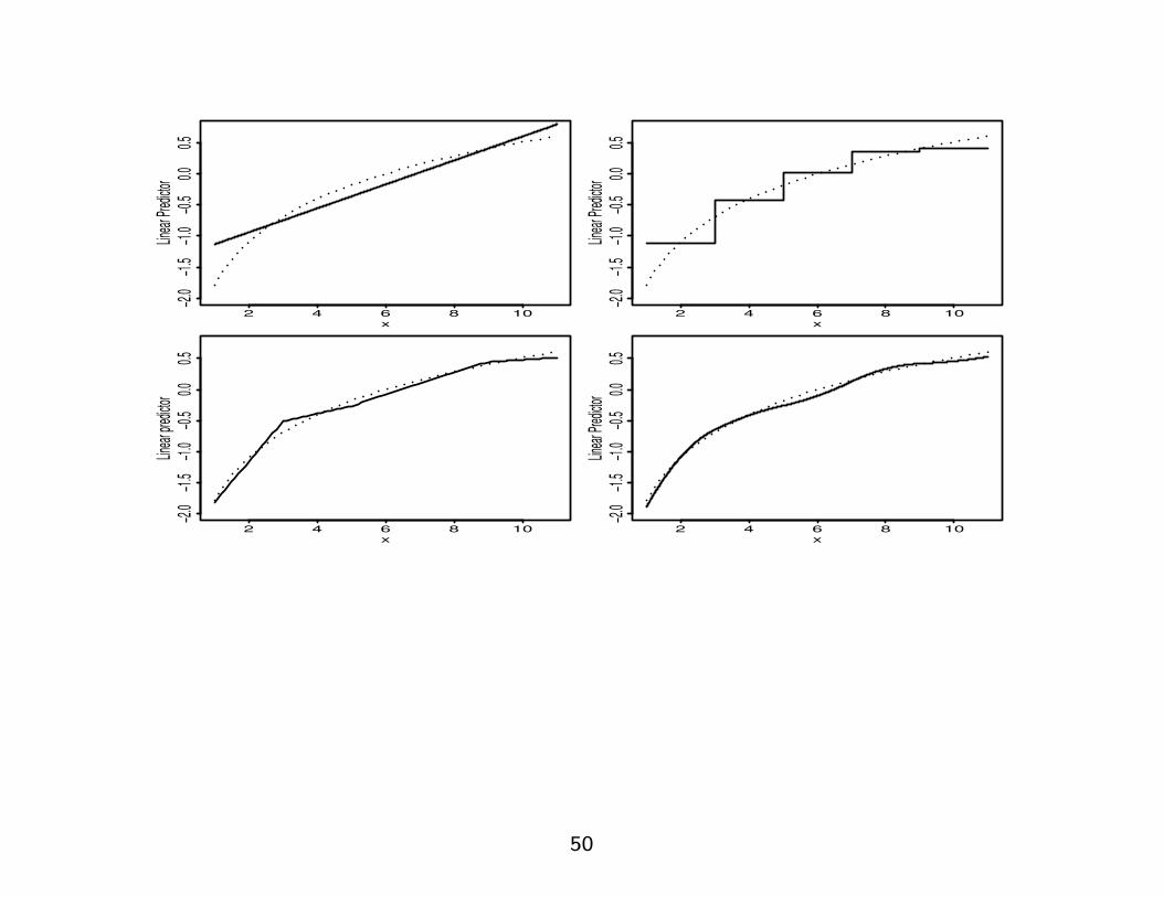
Linear splinesAn alternative to a straight line could be a broken line.

Introduce break points for x, e.g., a1, a2, a3 and add the three linearsplines

I1 × [x− a1], I2 × [x− a2], I3 × [x− a3]

to [x]:

Here, I1 = indicator for x ≥ a1I2 = indicator for x ≥ a2I3 = indicator for x ≥ a3

The parameter for the spline I1 × [x− a1] gives the change in slope atthe break point a1. Similarly for a2, a3.

Splines are easy to program and parameters are easier to interpret thanfor quadratic terms (quadratic and cubic splines also exist - but thenthe nice interpretation is lost).

49

2 4 6 8 10

−2.0

−1.5

−1.0

−0.5

0.00.5

x

Linea

r Pred

ictor

2 4 6 8 10

−2.0

−1.5

−1.0

−0.5

0.00.5

x

Linea

r Pred

ictor

2 4 6 8 10

−2.0

−1.5

−1.0

−0.5

0.00.5

x

Linea

r pred

ictor

2 4 6 8 10

−2.0

−1.5

−1.0

−0.5

0.00.5

x

Linea

r Pred

ictor

50

SAS code for indicator variables and splines (1)Indicator variables (Z0, Z1) in SAS may be created in the obvious wayfrom a binary variable Z:

if Z=0 then Z0=1; if Z=1 then Z0=0;

if Z=0 then Z1=0; if Z=1 then Z1=1;

A shorter, but less transparent code uses ‘logical expressions’:

Z0=(Z=0); Z1=(Z=1);

Then include either Z0 or Z1 in the model (depending on the preferredreference group).

51

SAS code for indicator variables and splines (2)The last way of coding makes creation of splines easy.

Suppose X is quantitative and we want a linear spline with breakpoints at A1 and A2:

X1=(X-A1)*(X>=A1); X2=(X-A2)*(X>=A2);

Then include both X, X1 and X2 in the model to obtain a piecewiselinear effect of X.

The test for linearity corresponds to eliminating both X1 and X2 fromthe model.

52

Ph.D.course2018:...

Documents

Transcript of Ph.D.course2018:...