PEAT8002 - SEISMOLOGY Lecture 6: Ray theoryrses.anu.edu.au › ~nick › teachdoc ›...

PEAT8002 - SEISMOLOGYLecture 6: Ray theory

Nick Rawlinson

Research School of Earth SciencesAustralian National University

Ray theoryIntroduction

Here, we consider the problem of how body waves (P andS) propagate through a medium in which the elasticparameters vary with spatial location.The elastic wave equation in a medium with spatiallyvariable properties is

ρu =∇λ(∇ · u) +∇µ · [∇u + (∇u)T] + (λ + 2µ)∇(∇ · u)

− µ∇×∇× u

The two terms containing ∇λ and ∇µ mean that P and Smotions do not decouple in heterogeneous media.


However, if the scale length of variations in λ and µ arelarge compared to the seismic wavelength, then P and Scan be treated separately and the elastic wave equation issimplified.Even so, solving the elastic wave equation requiresexhaustive computational effort.Ray theory is an alternative approach in which a point onthe wavefront is tracked rather than the complete wavefield.Ray theory is extensively used due to its simplicity, speedand applicability to a wide range of problems.


Ray theory is strictly valid for media whose length scalevariation of λ and µ is much larger than the seismicwavelength (the high frequency assumption).At low frequencies, diffraction and scattering can besignificant, and ray theory is not generally valid.Ray theory is an integral part of many seismologicaltechniques, including body wave tomography, migration ofreflection data, and earthquake relocation.The process of tracking the kinematic evolution of seismicenergy also brings with it the possibility of computing otherwave-related quantities such as traveltime, amplitude,attenuation, or even the high frequency waveform, whichcan then be compared to observations.

Ray theoryThe eikonal equation

Under the high frequency assumption, the full waveequation can be greatly simplified. Here, we consider thepropagation of P-waves in heterogeneous media.From before, the wave equation is:

∇2Φ− 1α2

∂2Φ

∂t2 = 0

where Φ represents the scalar potential of a P-wave.Now assume a harmonic solution of the form:

Φ = A(x)exp[−iω(T (x) + t)]

where T (x) is a phase function which describes thearbitrary distribution in space of a surface of constantphase.


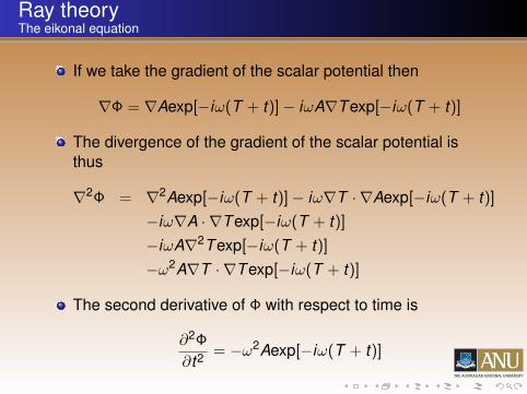
If we take the gradient of the scalar potential then

∇Φ = ∇Aexp[−iω(T + t)]− iωA∇Texp[−iω(T + t)]

The divergence of the gradient of the scalar potential isthus

∇2Φ = ∇2Aexp[−iω(T + t)]− iω∇T · ∇Aexp[−iω(T + t)]−iω∇A · ∇Texp[−iω(T + t)]−iωA∇2Texp[−iω(T + t)]−ω2A∇T · ∇Texp[−iω(T + t)]

The second derivative of Φ with respect to time is

∂2Φ

∂t2 = −ω2Aexp[−iω(T + t)]


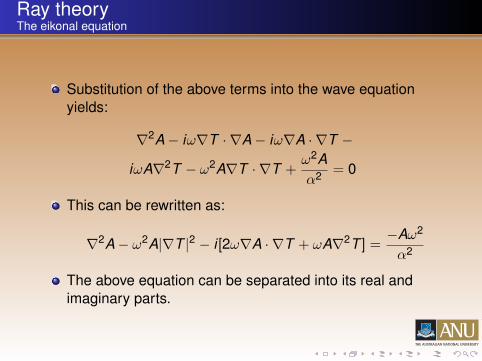
Substitution of the above terms into the wave equationyields:

∇2A− iω∇T · ∇A− iω∇A · ∇T −

iωA∇2T − ω2A∇T · ∇T +ω2Aα2 = 0

This can be rewritten as:

∇2A− ω2A|∇T |2 − i[2ω∇A · ∇T + ωA∇2T ] =−Aω2

α2

The above equation can be separated into its real andimaginary parts.


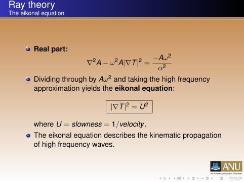
Real part:

∇2A− ω2A|∇T |2 =−Aω2

α2

Dividing through by Aω2 and taking the high frequencyapproximation yields the eikonal equation:

|∇T |2 = U2

where U = slowness = 1/velocity .The eikonal equation describes the kinematic propagationof high frequency waves.

Ray theoryThe transport equation

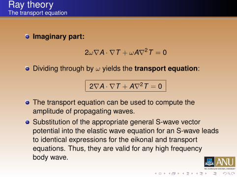
Imaginary part:

2ω∇A · ∇T + ωA∇2T = 0

Dividing through by ω yields the transport equation:

2∇A · ∇T + A∇2T = 0

The transport equation can be used to compute theamplitude of propagating waves.Substitution of the appropriate general S-wave vectorpotential into the elastic wave equation for an S-wave leadsto identical expressions for the eikonal and transportequations. Thus, they are valid for any high frequencybody wave.

Ray theoryWavefronts and rays

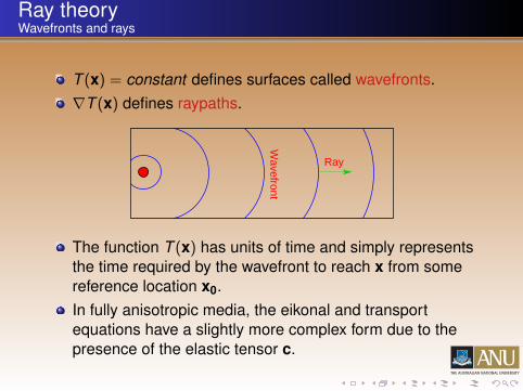
T (x) = constant defines surfaces called wavefronts.∇T (x) defines raypaths.

Wavefront

Ray

The function T (x) has units of time and simply representsthe time required by the wavefront to reach x from somereference location x0.In fully anisotropic media, the eikonal and transportequations have a slightly more complex form due to thepresence of the elastic tensor c.

Ray theoryThe kinematic ray tracing equations

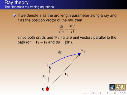
If we denote s as the arc length parameter along a ray andr as the position vector of the ray, then

drds

=∇TU

since both dr/ds and ∇T/U are unit vectors parallel to thepath (dr = r1 − r0 and ds = |dr|).

r1

s0

dr

0

0r

s1


The rate of change of traveltime along the path is simplydefined by the slowness, so

dTds

= U

If we take the gradient of both sides, then

d∇Tds

= ∇U (1)

noting the commutation of d/ds and ∇.From before,

∇T = Udrds

(2)


Combining Equations (1) and (2) produces

dds

[U

drds

]= ∇U

which is the kinematic ray equation and describes thetrajectory of ray paths in smoothly varying isotropic media.It will be shown later how this equation can be reduced toforms suitable for initial and boundary value ray tracing.The ray equation requires U to be differentiable, andtherefore is not applicable at the boundary between twomedia of different wavespeed.

Ray theoryFermat’s principle

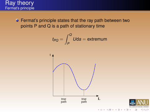
Fermat’s principle states that the ray path between twopoints P and Q is a path of stationary time

tPQ =

∫ Q

PUds = extremum

truepath

truepath

L

t


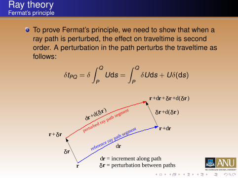
To prove Fermat’s principle, we need to show that when aray path is perturbed, the effect on traveltime is secondorder. A perturbation in the path perturbs the traveltime asfollows:

δtPQ = δ

∫ Q

PUds =

∫ Q

PδUds + Uδ(ds)

dr

δr

δr

r+dr

r+dr

δr

drδr

reference ray path segmentperturbed ray path segment

r+

rδ+ +d( )rδ

+d( )rδdr+d(

)rδ

r= increment along path= perturbation between paths


The first term in the integrand on the RHS is thecontribution caused by a change in velocity; the secondterm is the contribution caused by the change in pathlength.If we first consider the change in path length,

δ(ds) = |dr + d(δr)| − |dr|=

√dr · dr + 2dr · d(δr) + d(δr).d(δr)−

√dr · dr

=√

dr · dr + 2dr · d(δr)−√

dr · drsince |d(δr)| << |dr|

= ds

√1 +

2dr · d(δr)ds2 − ds

since ds =√

dr · dr

=drds

· d(δr)


The last equality arises from the fact that:[1 +

dr · d(δr)ds2

]2

= 1 +2dr · d(δr)

ds2 +d(δr)2

ds2

where the last term on the RHS is ≈ 0.The other term in the integrand, δU, is simply:

δU = ∇U · δr =∂U∂x

δx +∂U∂y

δy +∂U∂z

δz

where ∇U · δr is a directional derivative in δr direction.


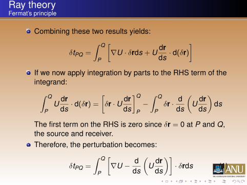
Combining these two results yields:

δtPQ =

∫ Q

P

[∇U · δrds + U

drds

· d(δr)]

If we now apply integration by parts to the RHS term of theintegrand:∫ Q

PU

drds

· d(δr) =

[δr · U dr

ds

]Q

P−

∫ Q

Pδr · d

ds

(U

drds

)ds

The first term on the RHS is zero since δr = 0 at P and Q,the source and receiver.Therefore, the perturbation becomes:

δtPQ =

∫ Q

P

[∇U − d

ds

(U

drds

)]· δrds (1)


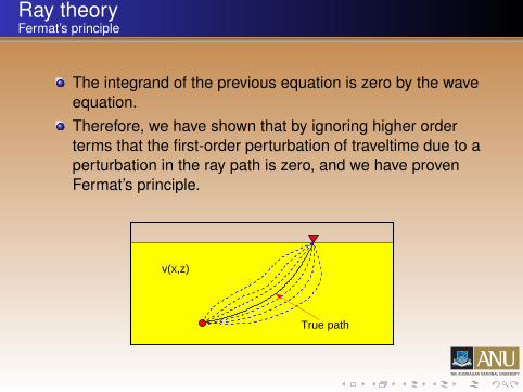
The integrand of the previous equation is zero by the waveequation.Therefore, we have shown that by ignoring higher orderterms that the first-order perturbation of traveltime due to aperturbation in the ray path is zero, and we have provenFermat’s principle.

True path

v(x,z)

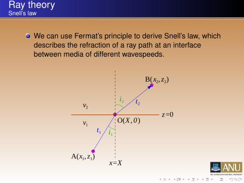
Ray theorySnell’s law

We can use Fermat’s principle to derive Snell’s law, whichdescribes the refraction of a ray path at an interfacebetween media of different wavespeeds.

x1

B( , z2)x2

i2 t2

i1t1

v1

x=X

=0zv2

A( , z1)

O( , 0X )


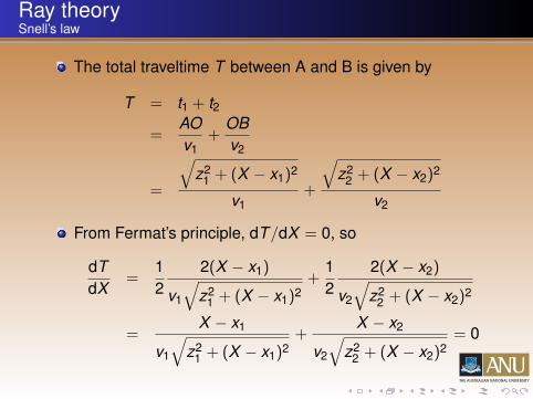
The total traveltime T between A and B is given by

T = t1 + t2

=AOv1

+OBv2

=

√z2

1 + (X − x1)2

v1+

√z2

2 + (X − x2)2

v2

From Fermat’s principle, dT/dX = 0, so

dTdX

=12

2(X − x1)

v1

√z2

1 + (X − x1)2+

12

2(X − x2)

v2

√z2

2 + (X − x2)2

=X − x1

v1

√z2

1 + (X − x1)2+

X − x2

v2

√z2

2 + (X − x2)2= 0


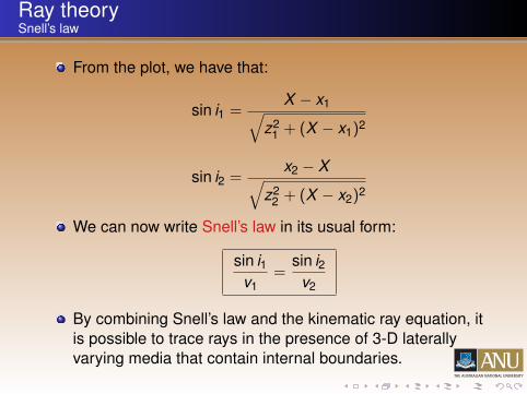
From the plot, we have that:

sin i1 =X − x1√

z21 + (X − x1)2

sin i2 =x2 − X√

z22 + (X − x2)2

We can now write Snell’s law in its usual form:

sin i1v1

=sin i2

v2

By combining Snell’s law and the kinematic ray equation, itis possible to trace rays in the presence of 3-D laterallyvarying media that contain internal boundaries.

PEAT8002 - SEISMOLOGY Lecture 6: Ray theoryrses.anu.edu.au › ~nick › teachdoc ›...

Documents

Transcript of PEAT8002 - SEISMOLOGY Lecture 6: Ray theoryrses.anu.edu.au › ~nick › teachdoc ›...