Parallel Hopfield Networks - University of Arizonabob/publications/2007_Cosyne_Wilson_poster.pdf ·...
1
0 0.1 0.2 0.3 0.4 0.5 0.6 0.7 0.8 0.9 1 0 0.1 0.2 0.3 0.4 0.5 0.6 0.7 0.8 0.9 1 P AM E SG α θ time step neuron number 200 400 600 800 50 100 150 200 250 300 350 400 450 500 period number neuron number 2 4 6 8 50 100 150 200 250 300 350 400 450 500 0 2 4 6 8 10 0 0.2 0.4 0.6 0.8 1 period number overlap with recalled memory time step neuron number 200 400 600 800 50 100 150 200 250 300 350 400 450 500 time step neuron number 200 400 600 800 50 100 150 200 250 300 350 400 450 500 Parallel Hopfield Networks Robert C. Wilson Department of Bioengineering, University of Pennsylvania Abstract We introduce a novel type of neural network, termed the Parallel Hopfield Net- work, that uses precise spike timing in order to simultaneously effect the dynamics of many different, independent Hopfield networks in parallel in the same piece of neural hardware. We analyze the network theoretically using an approximate set of self-consistent mean field equations which allows us to generate phase dia- grams for the network. Each Hopfield sub-network is found to have finite memory capacity as the number of neurons goes to infinity. Simulations with finite num- bers of neurons confirm the predictions of the theory. Order Parameters Using the method of self-consistent signal to noise analysis [1], it is possible to derive approximate mean field equations for the networks which are then de- scribed in terms of four order parameters: f - the frequency of spiking in the network which is further split into f gen - the rate of genuine spiking, and f sp - the frequency of spurious spiking m - the overlap of the subnetworks with the memories being recalled q - the Edwards-Anderson order parameter describing the level of spin glass ordering in the subnetworks r - which describes the level of random activation in the subnetworks. Acknowledgements We thank Leif Finkel, John Schotland, David MacKay and Seb Wills for inspiring conversations and excellent feedback. 0 0 0 0 0 0 0 0 0 0 0 0 0 1 0 0 neuron number 1 1 1 1 0 0 0 0 0 0 0 0 0 0 0 0 0 0 0 0 0 0 0 0 0 0 0 1 1 1 1 0 0 0 0 0 1 0 1 1 1 W i2 , τ i2 2 2 W i2 , τ i2 1 2 3 4 5 6 7 8 1 2 3 4 5 6 OR 1 conjunction detectors neuron 1 at time 8 1 0 8 time step 7 Σ Σ >θ? >θ? Activation rule Different spatio-temporal ‘memories’ (µ) hold different Hopfield-like sub-networks. Hopfield patterns (p) are generated randomly with the activity of the ith neuron in subnetwork µ and pattern p given by The weights are then given by the Hebb rule ... The update rule is outlined in the figure below period number neuron number 2 4 6 8 10 12 14 16 20 40 60 80 100 120 140 160 180 200 Input pattern 100 120 140 160 180 200 0 20 40 60 80 100 120 140 160 180 200 time step neuron number A B Simple demonstration This figure shows the results of a simultation of a PHN made up of 200 neurons, containing 9 different memories, each one loaded with 10 different Hopfield pat- terns. A shows 100 time steps of the simulation; the black dots correspond to neural spikes and the red boxes denote the spatio-temporal mask for one of the memories. B shows the activity at the mask points for this memory and compares it with the activity profile of the pattern being recalled. m q f sp r Phase Diagrams The mean field equations can be solved to produce phase diagrams which have four distinct regions - an associative memory phase AM, where the sub-networks act as attractors; an extinction phase E, where the network activity goes to zero; a spin-glass phase, SG, where each of the sub-networks shows spin glass order- ing; and a proliferation phase, P, where the activity of the network blows up. Above are the θ-α phase diagram for f gen = 0.01 showing the values of each of the order parameters. Simulation results showing behaviour of the network in the different regimes. Ob- taining a network with finite numbers of neurons in which the spin-glass glass state was reachable proved very difficult - hence there are no results illustrating this state. However, more detailed simulations showed found that the boundaries of the other phases were quite tight. Conclusions and Future Work We have presented a new type of neural network, termed the Parallel Hopfield Network that uses precise spike timing in order to enact multiple Hopfield net- works in parallel in the same network. The simplicity of the network opens it up to theoretical analysis using mean field approaches. Future work will address problems with the biological plausibility (such as ultra- high connectivity, neurons with both inhibitory and excitatory character, etc ...) of these networks in a similar manner to which these questions were addressed in the Hopfield network e.g. [2]. References [1] M. Shiino and T. Fukai. Phys. Rev. E. 48 (2):867-897, 1993 [2] H. Sompolinsky. Phys. Rev. A. 37:2571, 1986
Transcript of Parallel Hopfield Networks - University of Arizonabob/publications/2007_Cosyne_Wilson_poster.pdf ·...
0 0.1 0.2 0.3 0.4 0.5 0.6 0.7 0.8 0.9 10
0.1
0.2
0.3
0.4
0.5
0.6
0.7
0.8
0.9
1
P
AM
E
SG
α
θ
time step
neur
on n
umbe
r
200 400 600 800
50
100
150
200
250
300
350
400
450
500
period number
neur
on n
umbe
r
2 4 6 8
50
100
150
200
250
300
350
400
450
5000 2 4 6 8 10
0
0.2
0.4
0.6
0.8
1
period number
over
lap
with
reca
lled
mem
ory
time stepne
uron
num
ber
200 400 600 800
50
100
150
200
250
300
350
400
450
500
time step
neur
on n
umbe
r
200 400 600 800
50
100
150
200
250
300
350
400
450
500
Parallel Hopfield NetworksRobert C. Wilson
Department of Bioengineering, University of PennsylvaniaAbstract
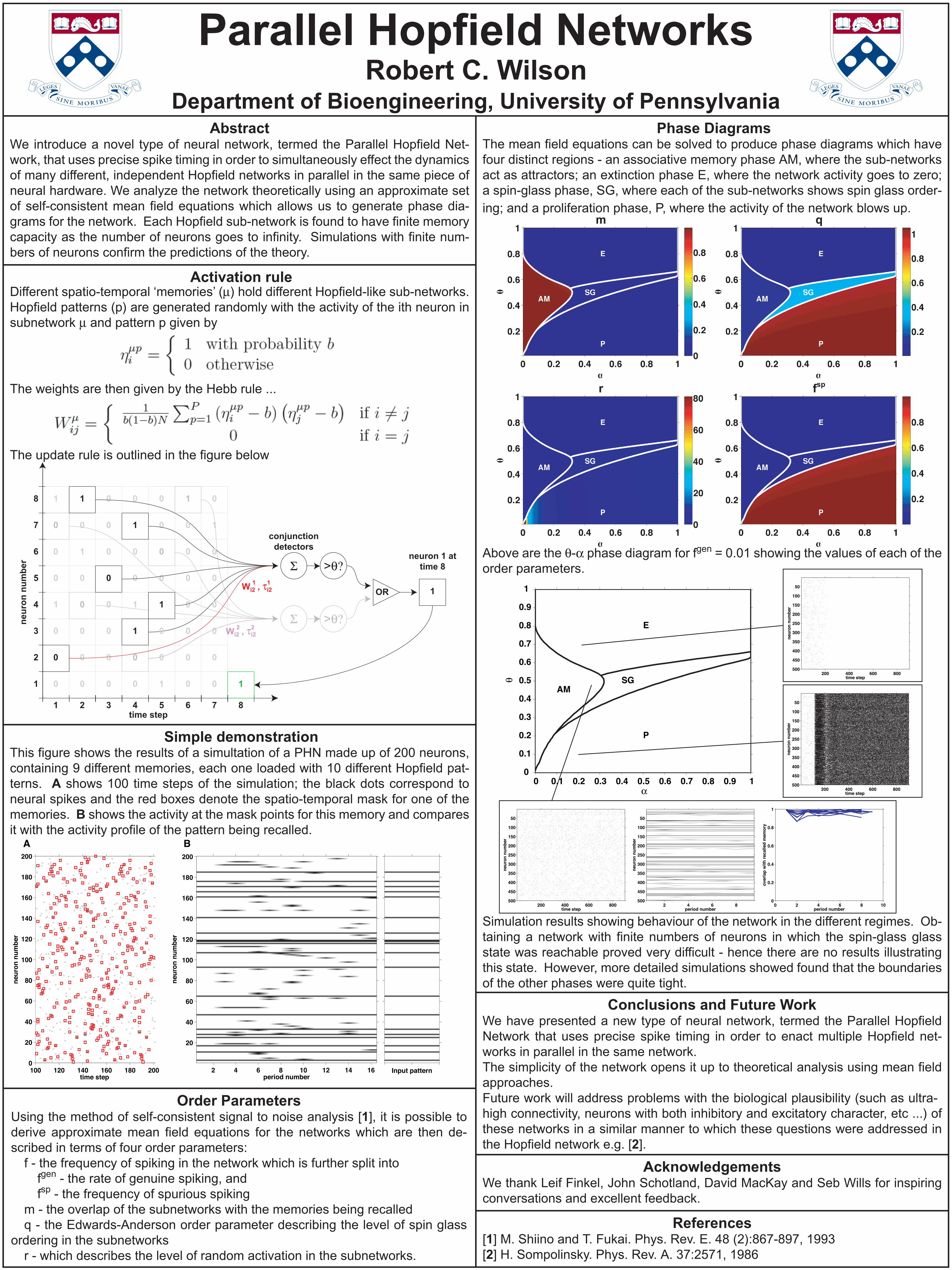
We introduce a novel type of neural network, termed the Parallel Hopfield Net-work, that uses precise spike timing in order to simultaneously effect the dynamics of many different, independent Hopfield networks in parallel in the same piece of neural hardware. We analyze the network theoretically using an approximate set of self-consistent mean field equations which allows us to generate phase dia-grams for the network. Each Hopfield sub-network is found to have finite memory capacity as the number of neurons goes to infinity. Simulations with finite num-bers of neurons confirm the predictions of the theory.
Order ParametersUsing the method of self-consistent signal to noise analysis [1], it is possible to derive approximate mean field equations for the networks which are then de-scribed in terms of four order parameters: f - the frequency of spiking in the network which is further split into fgen - the rate of genuine spiking, and fsp - the frequency of spurious spiking m - the overlap of the subnetworks with the memories being recalled q - the Edwards-Anderson order parameter describing the level of spin glass ordering in the subnetworks r - which describes the level of random activation in the subnetworks.
AcknowledgementsWe thank Leif Finkel, John Schotland, David MacKay and Seb Wills for inspiring conversations and excellent feedback.
00
0
0
00
0 0 0
0
0 0 0
1
00
neu
ron
nu
mb
er
1
1
1
1 0 0
0 0
0 0000
0 0
0
0
0 0
000
0 0
000
1
1
1
1
0
0 0
0
0
1
0 1
1 1
Wi2 , τi2
2 2
Wi2 , τi2
1
2
3
4
5
6
7
8
1 2 3 4 5 6
OR 1
conjunction detectors
neuron 1 at time 8
1
0
8time step
7
Σ
Σ
>θ?
>θ?
Activation ruleDifferent spatio-temporal ‘memories’ (µ) hold different Hopfield-like sub-networks. Hopfield patterns (p) are generated randomly with the activity of the ith neuron in subnetwork µ and pattern p given by
The weights are then given by the Hebb rule ...
The update rule is outlined in the figure below
period number
neur
on n
umbe
r
2 4 6 8 10 12 14 16
20
40
60
80
100
120
140
160
180
200
Input pattern100 120 140 160 180 2000
20
40
60
80
100
120
140
160
180
200
time step
neur
on n
umbe
r
A B
Simple demonstrationThis figure shows the results of a simultation of a PHN made up of 200 neurons, containing 9 different memories, each one loaded with 10 different Hopfield pat-terns. A shows 100 time steps of the simulation; the black dots correspond to neural spikes and the red boxes denote the spatio-temporal mask for one of the memories. B shows the activity at the mask points for this memory and compares it with the activity profile of the pattern being recalled.
m q
fspr
Phase DiagramsThe mean field equations can be solved to produce phase diagrams which have four distinct regions - an associative memory phase AM, where the sub-networks act as attractors; an extinction phase E, where the network activity goes to zero; a spin-glass phase, SG, where each of the sub-networks shows spin glass order-ing; and a proliferation phase, P, where the activity of the network blows up.
Above are the θ-α phase diagram for fgen = 0.01 showing the values of each of the order parameters.
Simulation results showing behaviour of the network in the different regimes. Ob-taining a network with finite numbers of neurons in which the spin-glass glass state was reachable proved very difficult - hence there are no results illustrating this state. However, more detailed simulations showed found that the boundaries of the other phases were quite tight.
Conclusions and Future WorkWe have presented a new type of neural network, termed the Parallel Hopfield Network that uses precise spike timing in order to enact multiple Hopfield net-works in parallel in the same network. The simplicity of the network opens it up to theoretical analysis using mean field approaches.Future work will address problems with the biological plausibility (such as ultra-high connectivity, neurons with both inhibitory and excitatory character, etc ...) of these networks in a similar manner to which these questions were addressed in the Hopfield network e.g. [2].
References[1] M. Shiino and T. Fukai. Phys. Rev. E. 48 (2):867-897, 1993[2] H. Sompolinsky. Phys. Rev. A. 37:2571, 1986