neural network lecture 3

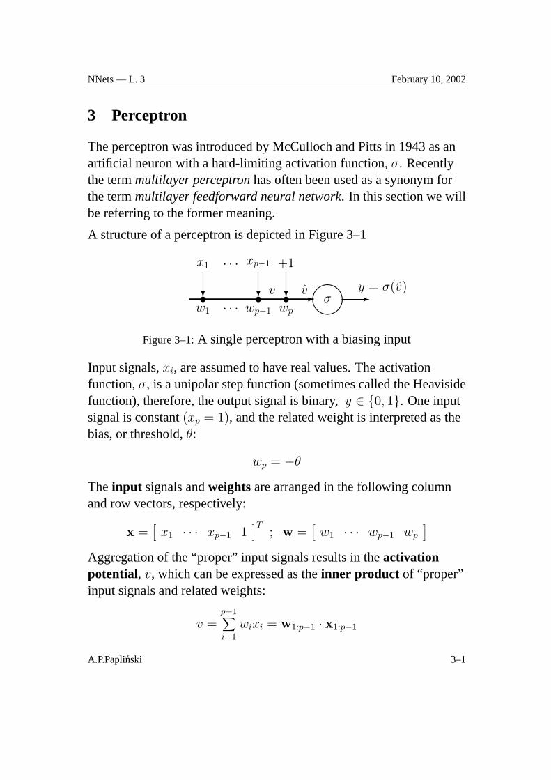
NNets — L. 3 February 10, 2002

3 Perceptron

The perceptron was introduced by McCulloch and Pitts in 1943 as anartificial neuron with a hard-limiting activation function,σ. Recentlythe termmultilayer perceptronhas often been used as a synonym forthe termmultilayer feedforward neural network. In this section we willbe referring to the former meaning.

A structure of a perceptron is depicted in Figure 3–1

��

σ -v v y = σ(v)u u u

w1 . . . wp−1 wp

? ? ?

x1 · · · xp−1 +1

-

Figure 3–1:A single perceptron with a biasing input

Input signals,xi, are assumed to have real values. The activationfunction,σ, is a unipolar step function (sometimes called the Heavisidefunction), therefore, the output signal is binary,y ∈ {0, 1}. One inputsignal is constant(xp = 1), and the related weight is interpreted as thebias, or threshold,θ:

wp = −θ

The input signals andweightsare arranged in the following columnand row vectors, respectively:

x =[

x1 · · · xp−1 1]T

; w =[

w1 · · · wp−1 wp

]Aggregation of the “proper” input signals results in theactivationpotential, v, which can be expressed as theinner product of “proper”input signals and related weights:

v =p−1∑i=1

wixi = w1:p−1 · x1:p−1

A.P.Paplinski 3–1


The augmented activation potential,v, can now be expressed simply as:

v = w · x = v − θ

For each input signal, the output is determined as

y = σ(v) =

0 if v < θ (v < 0)1 if v ≥ θ (v ≥ 0)

Hence, a perceptron works as athreshold element, the output being“active” if the activation potential exceeds the threshold.

3.1 A Perceptron as a Pattern Classifier

A single perceptron classifies input patterns,x, into two classes.

A linear combination of signals and weights for which the augmentedactivation potential is zero,v = 0, describes adecision surfacewhichpartitions the input space into two regions. The decision surface is ahyperplanespecified as:

w · x = 0 , xp = 1 , or v = θ (3.1)

and we say that an input vector (pattern)

x belongs to a class

#1#0

if

y = 1, (v ≥ θ)y = 0, (v < θ)

The input patterns that can be classified by a single perceptron into twodistinct classes are calledlinearly separable patterns.

A.P.Paplinski 3–2


Useful remarks

• The inner product of two vectors can be also expressed as:

w · x = ||w|| · ||x|| · cos α

where||.|| denotes the norm (magnitude, length) of the vector,andα is the angle between vectors.

• The weight vector,w, is orthogonal to the decision plane in theaugmented input space, because

w · x = 0

that is, the inner product of the weight and augmented inputvectors is zero.

• Note that the weight vector,

w1:p−1

is also orthogonal to the decision plane

w1:p−1 · x1:p−1 + wp = 0

in the “proper”,(p−1)–dimensional input space. For any pair ofinput vectors, say,(xa

1:p−1,xb1:p−1), for which the decision plane

equation is satisfied, we have

w1:p−1 · (xa1:p−1 − xb

1:p−1) = 0

Note that the difference vector(xa1:p−1 − xb

1:p−1) lies in thedecision plane.

A.P.Paplinski 3–3


Geometric Interpretation

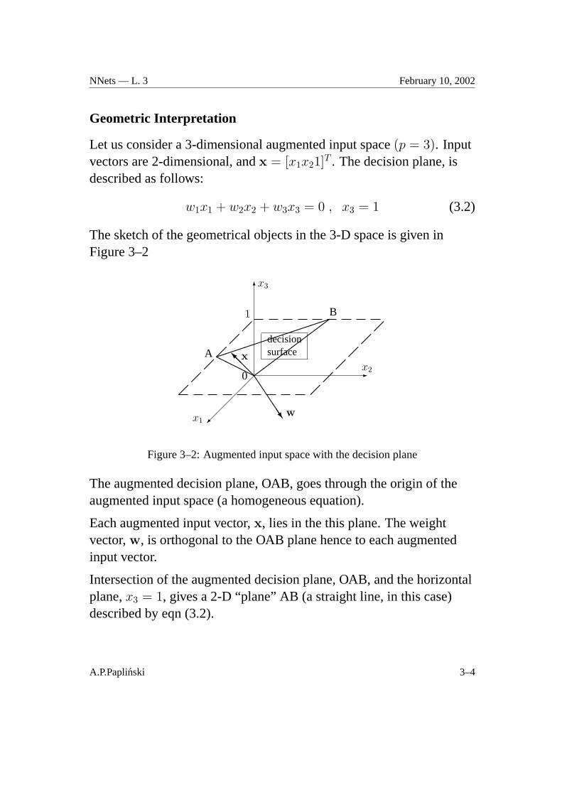
Let us consider a 3-dimensional augmented input space(p = 3). Inputvectors are 2-dimensional, andx = [x1x21]T . The decision plane, isdescribed as follows:

w1x1 + w2x2 + w3x3 = 0 , x3 = 1 (3.2)

The sketch of the geometrical objects in the 3-D space is given inFigure 3–2

6x3

��

��

�x1

-x2

decisionsurface

HHHH

��

��

��

��

��1

0

A

B

�

�

�

�

�

�

�

�

�

�

�

�

JJ

JJJ w

@@@Ix

Figure 3–2: Augmented input space with the decision plane

The augmented decision plane, OAB, goes through the origin of theaugmented input space (a homogeneous equation).

Each augmented input vector,x, lies in the this plane. The weightvector,w, is orthogonal to the OAB plane hence to each augmentedinput vector.

Intersection of the augmented decision plane, OAB, and the horizontalplane,x3 = 1, gives a 2-D “plane” AB (a straight line, in this case)described by eqn (3.2).

A.P.Paplinski 3–4


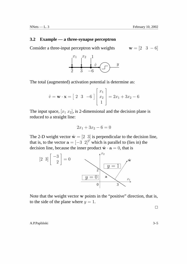
3.2 Example — a three-synapse perceptron

Consider a three-input perceptron with weights w = [2 3 − 6]

v

��

yu u u? ? ?

x1 x2 1

2 3 −6-

The total (augmented) activation potential is determine as:

v = w · x =[

2 3 −6]

x1

x2

1

= 2x1 + 3x2 − 6

The input space,[x1 x2], is 2-dimensional and the decision plane isreduced to a straight line:

2x1 + 3x2 − 6 = 0

The 2-D weight vectorw = [2 3] is perpendicular to the decision line,that is, to the vectora = [−3 2]T which is parallel to (lies in) thedecision line, because the inner productw · a = 0, that is

[2 3]

−32

= 0

-x1

6x2

0 3

2y = 1

y = 0

�w

a

QQ

QQ

QQ

QQ

QQ

QQ

Q

Note that the weight vectorw points in the “positive” direction, that is,to the side of the plane wherey = 1.

2

A.P.Paplinski 3–5


3.3 Selection of weights for the perceptron

In order for the perceptron to perform a desired task, its weights mustbe properly selected.

In general two basic methods can be employed to select a suitableweight vector:

• By off-line calculation of weights. If the problem is relativelysimple it is often possible to calculate the weight vector from thespecification of the problem.

• By learning procedure. The weight vector is determined from agiven (training) set of input-output vectors (exemplars) in such away to achieve the best classification of the training vectors.

Once the weights are selected (theencoding process),the perceptron performs its desired task (e.g., pattern classification)(thedecoding process).

A.P.Paplinski 3–6


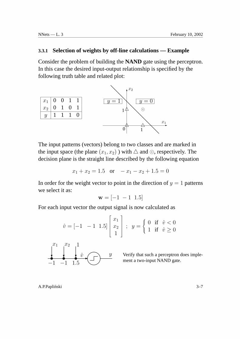
3.3.1 Selection of weights by off-line calculations — Example

Consider the problem of building theNAND gate using the perceptron.In this case the desired input-output relationship is specified by thefollowing truth table and related plot:

x1 0 0 1 1x2 0 1 0 1y 1 1 1 0

-x1

6x2

0 1

1

4 4

4 �y = 1 y = 0

@@

@@

@@

@@

@@

@@

The input patterns (vectors) belong to two classes and are marked inthe input space (the plane(x1, x2) ) with 4 and�, respectively. Thedecision plane is the straight line described by the following equation

x1 + x2 = 1.5 or − x1 − x2 + 1.5 = 0

In order for the weight vector to point in the direction ofy = 1 patternswe select it as:

w = [−1 − 1 1.5]

For each input vector the output signal is now calculated as

v = [−1 − 1 1.5]

x1

x2

1

; y =

0 if v < 01 if v ≥ 0

v

��

yu u u? ? ?

x1 x2 1

−1 −1 1.5-

Verify that such a perceptron does imple-ment a two-input NAND gate.

A.P.Paplinski 3–7


3.4 The Perceptron learning law

Learning is a recursive procedure of modifying weights from a givenset of input-output patterns.

For a single perceptron, the objective of the learning (encoding)procedure is to find the decision plane, (that is, the related weightvector), which separates two classes of giveninput-output trainingvectors.

Once the learning is finalised, every input vector will be classified intoan appropriate class. A single perceptron can classify only thelinearlyseparablepatterns.

The perceptron learning procedure is an example of asupervisederror-correcting learning law.

A.P.Paplinski 3–8


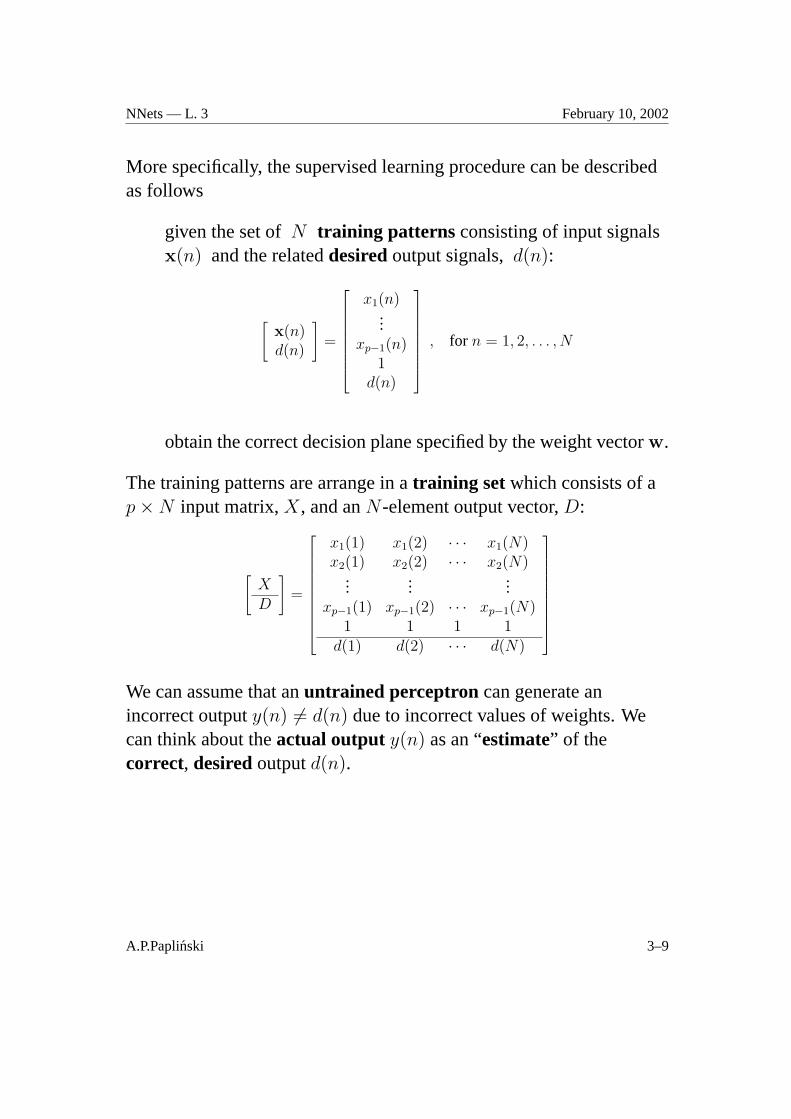
More specifically, the supervised learning procedure can be describedas follows

given the set ofN training patterns consisting of input signalsx(n) and the relateddesiredoutput signals,d(n):

[x(n)d(n)

]=

x1(n)...

xp−1(n)1

d(n)

, for n = 1, 2, . . . , N

obtain the correct decision plane specified by the weight vectorw.

The training patterns are arrange in atraining set which consists of ap×N input matrix,X, and anN -element output vector,D:

[XD

]=

x1(1) x1(2) · · · x1(N)x2(1) x2(2) · · · x2(N)

......

...xp−1(1) xp−1(2) · · · xp−1(N)

1 1 1 1d(1) d(2) · · · d(N)

We can assume that anuntrained perceptron can generate anincorrect outputy(n) 6= d(n) due to incorrect values of weights. Wecan think about theactual output y(n) as an “estimate” of thecorrect, desiredoutputd(n).

A.P.Paplinski 3–9


Theperceptron learning law proposed by Rosenblatt in 1959 alsoknown as theperceptron convergence procedure, can be described asfollows

1. weights are initially set to “small” random values

w(0) = rand

2. for n = 1, 2, . . . , N training input vectors,x(n), are presentedto the perceptron and theactual output y(n), is compared withthedesired output, d(n), and theerror ε(n) is calculated asfollows

y(n) = σ(w(n) · x(n)) , ε(n) = d(n)− y(n)

Note that because

d(n), y(n) ∈ {0, 1}, then ε(n) ∈ {−1, 0, +1}

3. at each step, the weights are adapted as follows

w(n + 1) = w(n) + η ε(n)x(n) (3.3)

where0 < η < 1 is a learning parameter (gain), which controlsthe adaptation rate. The gain must be adjusted to ensure theconvergence of the algorithm.

Note that the weight update

∆w = η ε(n)x(n) (3.4)

is zero if the errorε(n) = 0.

A.P.Paplinski 3–10


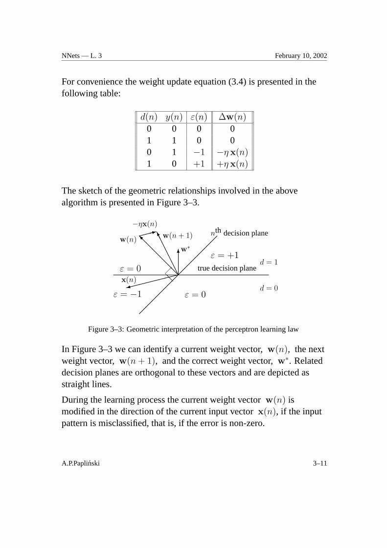
For convenience the weight update equation (3.4) is presented in thefollowing table:

d(n) y(n) ε(n) ∆w(n)

0 0 0 01 1 0 00 1 −1 −η x(n)1 0 +1 +η x(n)

The sketch of the geometric relationships involved in the abovealgorithm is presented in Figure 3–3.

�@@

true decision planed = 1

d = 0

��

��

��

��

��

��nth decision plane

��9x(n)

@@

@@

@@Iw(n)��:

−ηx(n)

AA

AA

AAAK w(n + 1)

6w∗

ε = −1

ε = 0

ε = 0

ε = +1

Figure 3–3: Geometric interpretation of the perceptron learning law

In Figure 3–3 we can identify a current weight vector,w(n), the nextweight vector,w(n + 1), and the correct weight vector,w∗. Relateddecision planes are orthogonal to these vectors and are depicted asstraight lines.

During the learning process the current weight vectorw(n) ismodified in the direction of the current input vectorx(n), if the inputpattern is misclassified, that is, if the error is non-zero.



Presenting the perceptron with enough training vectors, the weightvectorw(n) will tend to the correct valuew∗.

Rosenblatt proved that if input patterns are linearly separable, then theperceptron learning law converges, and the hyperplane separating twoclasses of input patterns can be determined.

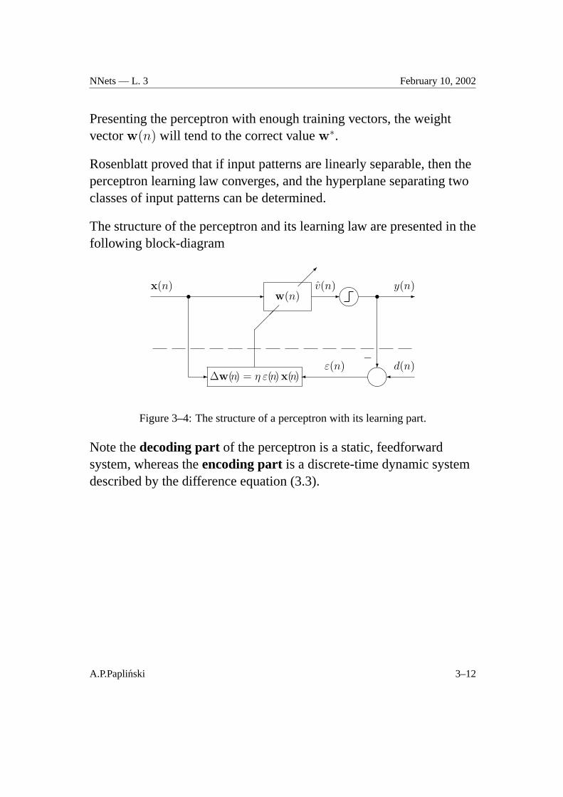
The structure of the perceptron and its learning law are presented in thefollowing block-diagram

-x(n)

w(n) ��

��

-v(n)

-y(n)s s

∆w(n) = η ε(n)x(n)-

��

��

?−

�d(n)

�ε(n)

Figure 3–4: The structure of a perceptron with its learning part.

Note thedecoding partof the perceptron is a static, feedforwardsystem, whereas theencoding part is a discrete-time dynamic systemdescribed by the difference equation (3.3).



3.5 Implementation of the perceptron learning law inMATLAB—Example

The following numerical example demonstrates the perceptronlearning law. In the example we will demonstrate three main stepstypical to most of the neural network applications, namely:

Preparation of the training patterns. Normally, the training patternsare specific to the particular application. In our example wegenerate a set of vectors and partition this set with a plane intotwo linearly separable classes. The set of vectors is split into twohalves, one used as atraining set, the other as avalidation set.

Learning. Using the training set, we apply the perceptron learning lawas described in sec. 3.4

Validation. Using the validation set we verify the quality of thelearning process.

Calculations are performed inMATLAB.



Description of a demo script perc.m

p = 5; % dimensionality of the augmented input space

N = 50; % number of training patterns — size of the training epoch

PART 1: Generation of the training and validation sets

X = 2*rand(p-1,2*N)-1; % a(p− 1)× 2N matrix ofuniformly distributed random numbers from the interval[−1, +1]

nn = round((2*N-1)*rand(N,1))+1; % generation ofNrandom integer numbers from the range[1..2N ]. Repetitions arepossible.

X(:,nn) = sin(X(:,nn)); % Columns of the matrix Xpointed to bynn are ”coloured” with the function ‘sin’, in orderto make the training patterns more interesting.

X = [X; ones(1,2*N)]; % Each input vector is appended witha constant 1 to implement biasing.

Comment: to generateN integer indices from[1..2N ] withoutrepetition use:

[srt,nn] = sort(rand(1,2*N)); nn=nn(1:N);

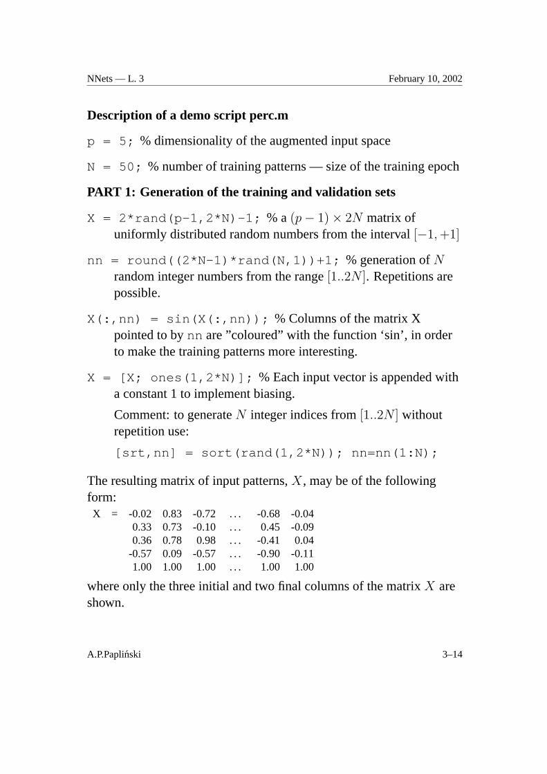
The resulting matrix of input patterns,X, may be of the followingform:X = -0.02 0.83 -0.72 . . . -0.68 -0.04

0.33 0.73 -0.10 . . . 0.45 -0.090.36 0.78 0.98 . . . -0.41 0.04

-0.57 0.09 -0.57 . . . -0.90 -0.111.00 1.00 1.00 . . . 1.00 1.00

where only the three initial and two final columns of the matrixX areshown.



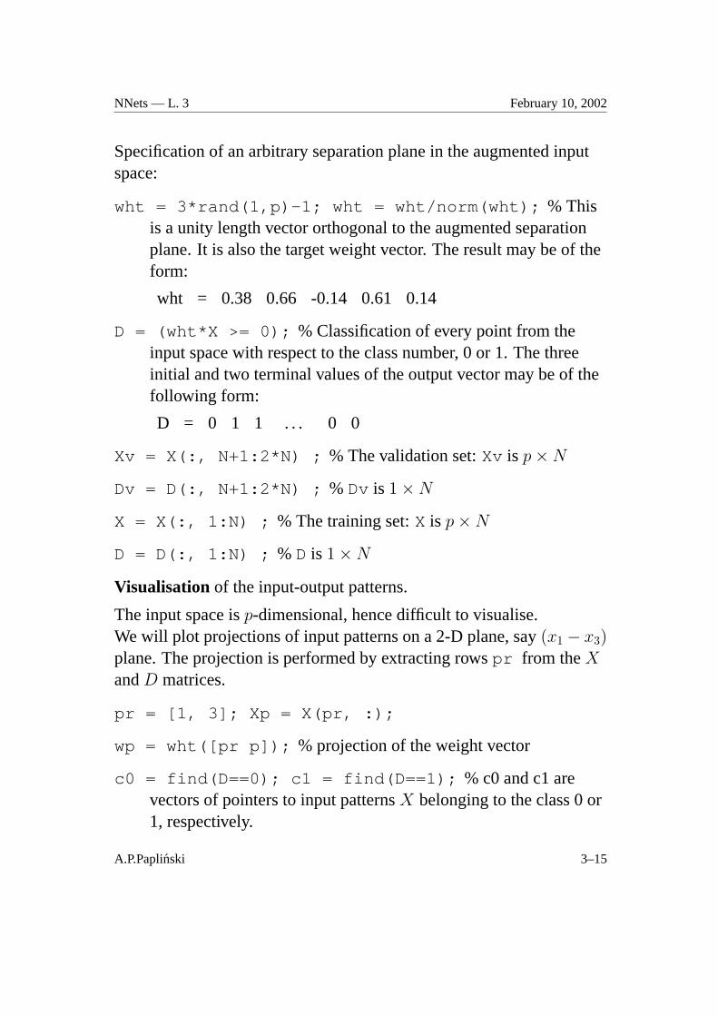
Specification of an arbitrary separation plane in the augmented inputspace:

wht = 3*rand(1,p)-1; wht = wht/norm(wht); % Thisis a unity length vector orthogonal to the augmented separationplane. It is also the target weight vector. The result may be of theform:

wht = 0.38 0.66 -0.14 0.61 0.14

D = (wht*X >= 0); % Classification of every point from theinput space with respect to the class number, 0 or 1. The threeinitial and two terminal values of the output vector may be of thefollowing form:

D = 0 1 1 . . . 0 0

Xv = X(:, N+1:2*N) ; % The validation set:Xv is p×N

Dv = D(:, N+1:2*N) ; % Dv is 1×N

X = X(:, 1:N) ; % The training set:X is p×N

D = D(:, 1:N) ; % D is 1×N

Visualisation of the input-output patterns.

The input space isp-dimensional, hence difficult to visualise.We will plot projections of input patterns on a 2-D plane, say(x1 − x3)plane. The projection is performed by extracting rowspr from theX

andD matrices.

pr = [1, 3]; Xp = X(pr, :);

wp = wht([pr p]); % projection of the weight vector

c0 = find(D==0); c1 = find(D==1); % c0 and c1 arevectors of pointers to input patternsX belonging to the class 0 or1, respectively.



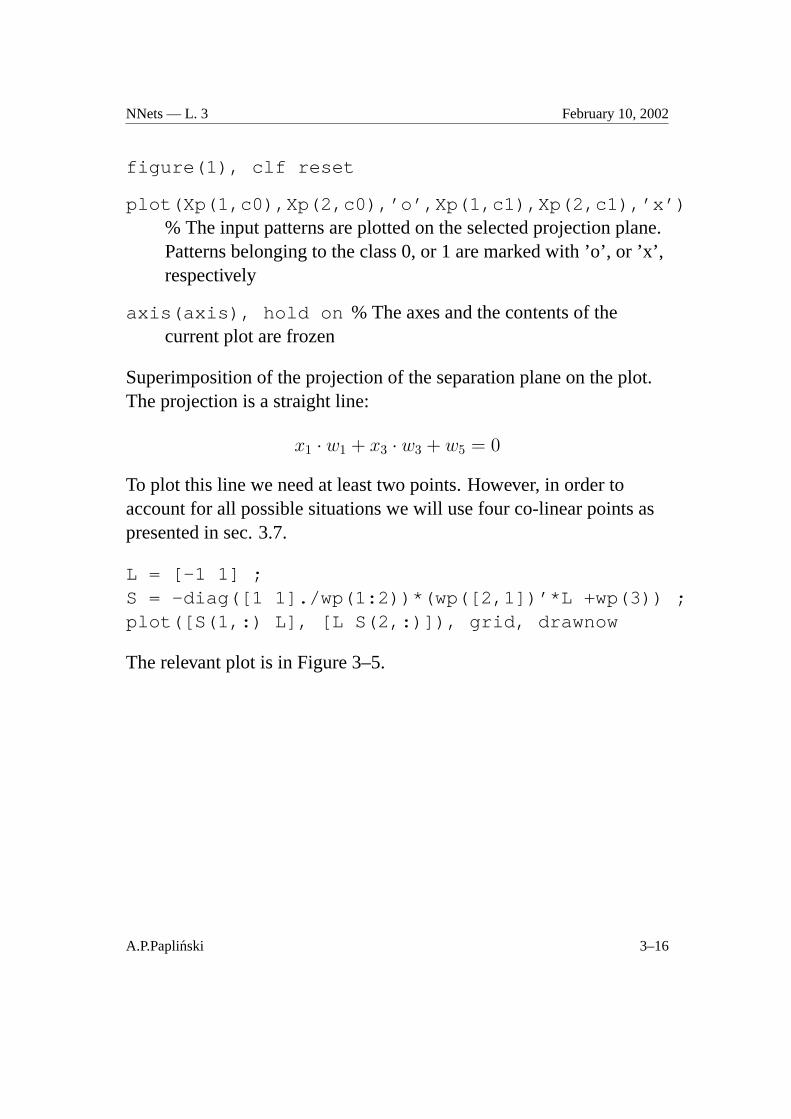
figure(1), clf reset

plot(Xp(1,c0),Xp(2,c0),’o’,Xp(1,c1),Xp(2,c1),’x’)% The input patterns are plotted on the selected projection plane.Patterns belonging to the class 0, or 1 are marked with ’o’, or ’x’,respectively

axis(axis), hold on % The axes and the contents of thecurrent plot are frozen

Superimposition of the projection of the separation plane on the plot.The projection is a straight line:

x1 · w1 + x3 · w3 + w5 = 0

To plot this line we need at least two points. However, in order toaccount for all possible situations we will use four co-linear points aspresented in sec. 3.7.

L = [-1 1] ;S = -diag([1 1]./wp(1:2))*(wp([2,1])’*L +wp(3)) ;plot([S(1,:) L], [L S(2,:)]), grid, drawnow

The relevant plot is in Figure 3–5.



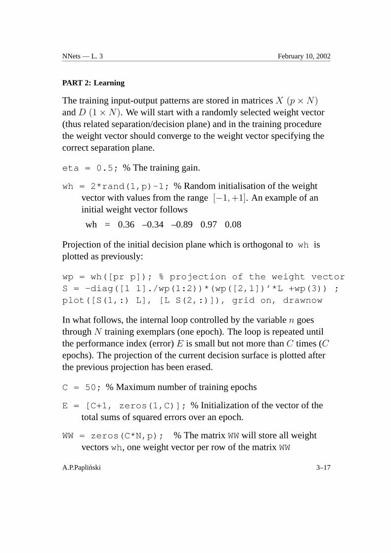
PART 2: Learning

The training input-output patterns are stored in matricesX (p×N)andD (1×N). We will start with a randomly selected weight vector(thus related separation/decision plane) and in the training procedurethe weight vector should converge to the weight vector specifying thecorrect separation plane.

eta = 0.5; % The training gain.

wh = 2*rand(1,p)-1; % Random initialisation of the weightvector with values from the range[−1, +1]. An example of aninitial weight vector follows

wh = 0.36 –0.34 –0.89 0.97 0.08

Projection of the initial decision plane which is orthogonal towh isplotted as previously:

wp = wh([pr p]); % projection of the weight vectorS = -diag([1 1]./wp(1:2))*(wp([2,1])’*L +wp(3)) ;plot([S(1,:) L], [L S(2,:)]), grid on, drawnow

In what follows, the internal loop controlled by the variablen goesthroughN training exemplars (one epoch). The loop is repeated untilthe performance index (error)E is small but not more thanC times (Cepochs). The projection of the current decision surface is plotted afterthe previous projection has been erased.

C = 50; % Maximum number of training epochs

E = [C+1, zeros(1,C)]; % Initialization of the vector of thetotal sums of squared errors over an epoch.

WW = zeros(C*N,p); % The matrixWWwill store all weightvectorswh, one weight vector per row of the matrixWW



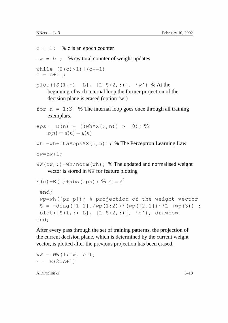
c = 1; % c is an epoch counter

cw = 0 ; % cw total counter of weight updates

while (E(c)>1)|(c==1)c = c+1 ;

plot([S(1,:) L], [L S(2,:)], ’w’) % At thebeginning of each internal loop the former projection of thedecision plane is erased (option ’w’)

for n = 1:N % The internal loop goes once through all trainingexemplars.

eps = D(n) - ((wh*X(:,n)) >= 0); %ε(n) = d(n)− y(n)

wh =wh+eta*eps*X(:,n)’; % The Perceptron Learning Law

cw=cw+1;

WW(cw,:)=wh/norm(wh); % The updated and normalised weightvector is stored inWWfor feature plotting

E(c)=E(c)+abs(eps); % |ε| = ε2

end;wp=wh([pr p]); % projection of the weight vectorS = -diag([1 1]./wp(1:2))*(wp([2,1])’*L +wp(3)) ;plot([S(1,:) L], [L S(2,:)], ’g’), drawnow

end;

After every pass through the set of training patterns, the projection ofthe current decision plane, which is determined by the current weightvector, is plotted after the previous projection has been erased.

WW = WW(1:cw, pr);E = E(2:c+1)



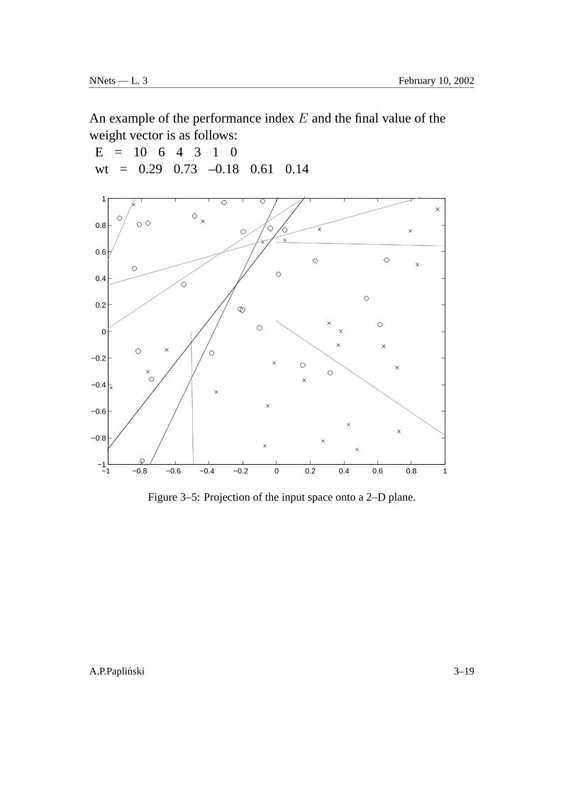
An example of the performance indexE and the final value of theweight vector is as follows:E = 10 6 4 3 1 0wt = 0.29 0.73 –0.18 0.61 0.14

−1 −0.8 −0.6 −0.4 −0.2 0 0.2 0.4 0.6 0.8 1−1

−0.8

−0.6

−0.4

−0.2

0

0.2

0.4

0.6

0.8

1

Figure 3–5: Projection of the input space onto a 2–D plane.



Validation

The final decision (separation) planes differs slightly from the correctone. Therefore, if we use input signals from the validation set whichwere not used in training, it may be expected that some patterns will bemisclassified and the following total sum of squared errors will benon-zero.

Ev = sum(abs(Dv - (wh*Xv >= 0))’)

The values ofEv over many training sessions were between 0 and 5(out ofN = 50).



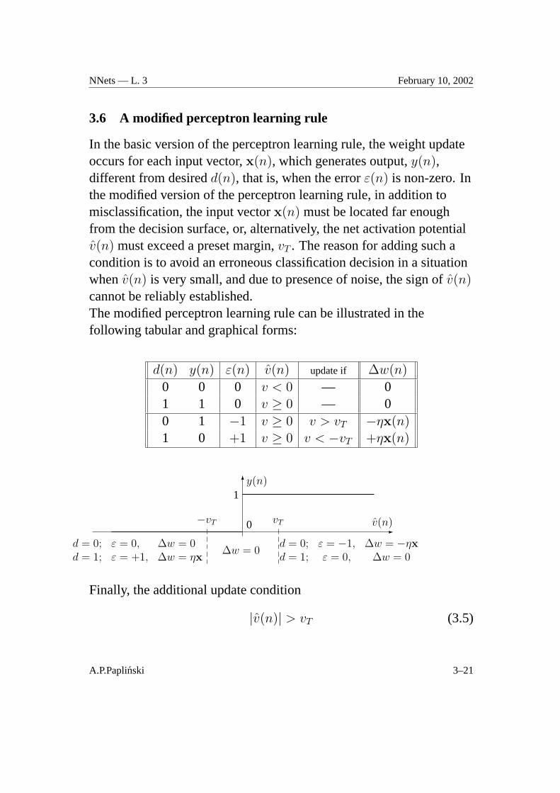
3.6 A modified perceptron learning rule

In the basic version of the perceptron learning rule, the weight updateoccurs for each input vector,x(n), which generates output,y(n),different from desiredd(n), that is, when the errorε(n) is non-zero. Inthe modified version of the perceptron learning rule, in addition tomisclassification, the input vectorx(n) must be located far enoughfrom the decision surface, or, alternatively, the net activation potentialv(n) must exceed a preset margin,vT . The reason for adding such acondition is to avoid an erroneous classification decision in a situationwhenv(n) is very small, and due to presence of noise, the sign ofv(n)cannot be reliably established.The modified perceptron learning rule can be illustrated in thefollowing tabular and graphical forms:

d(n) y(n) ε(n) v(n) update if ∆w(n)

0 0 0 v < 0 — 01 1 0 v ≥ 0 — 00 1 −1 v ≥ 0 v > vT −ηx(n)1 0 +1 v ≥ 0 v < −vT +ηx(n)

d = 0; ε = 0, ∆w = 0d = 1; ε = +1, ∆w = ηx

∆w = 0d = 0; ε = −1, ∆w = −ηxd = 1; ε = 0, ∆w = 0

-

6

−vT 0 vT

1y(n)

v(n)

Finally, the additional update condition

|v(n)| > vT (3.5)



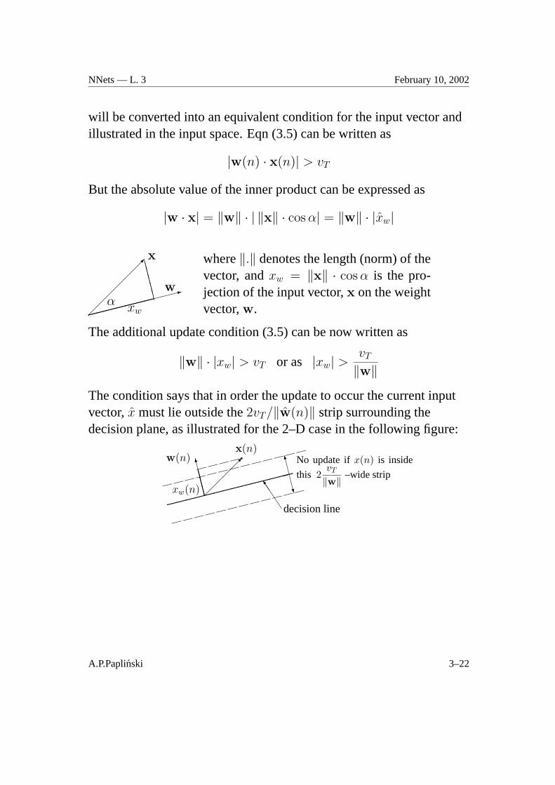
will be converted into an equivalent condition for the input vector andillustrated in the input space. Eqn (3.5) can be written as

|w(n) · x(n)| > vT

But the absolute value of the inner product can be expressed as

|w · x| = ‖w‖ · | ‖x‖ · cos α| = ‖w‖ · |xw|

��:

��

��

��CC

CCCCCCCC

wα

x

xw��

where‖.‖ denotes the length (norm) of thevector, andxw = ‖x‖ · cos α is the pro-jection of the input vector,x on the weightvector,w.

The additional update condition (3.5) can be now written as

‖w‖ · |xw| > vT or as |xw| >vT

‖w‖

The condition says that in order the update to occur the current inputvector,x must lie outside the2vT/‖w(n)‖ strip surrounding thedecision plane, as illustrated for the 2–D case in the following figure:

� � � � � � � � � � � � �

� � � � � � � � � � � �CCCCO

��

��

q� � � �

x(n)w(n)

xw(n)

CCO

CCW

No update ifx(n) is inside

this 2vT

‖w‖–wide strip

decision lineJJ

JJ]

��

CCC



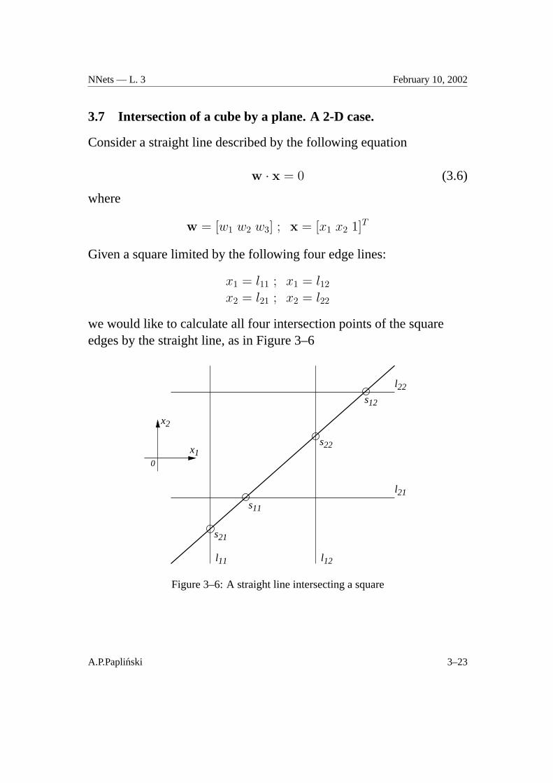
3.7 Intersection of a cube by a plane. A 2-D case.

Consider a straight line described by the following equation

w · x = 0 (3.6)

where

w = [w1 w2 w3] ; x = [x1 x2 1]T

Given a square limited by the following four edge lines:

x1 = l11 ; x1 = l12

x2 = l21 ; x2 = l22

we would like to calculate all four intersection points of the squareedges by the straight line, as in Figure 3–6

l22

l11 l12

l21

x1

x2

0

21

11

22

12

s

s

s

s

Figure 3–6: A straight line intersecting a square



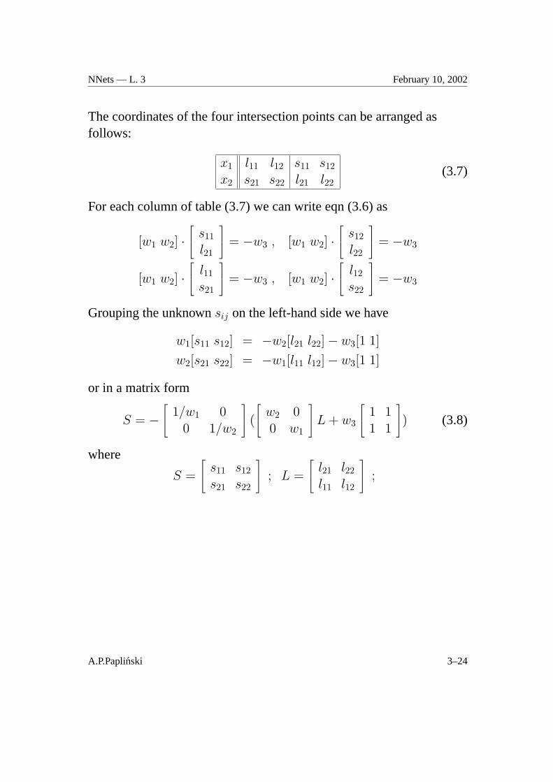
The coordinates of the four intersection points can be arranged asfollows:

x1 l11 l12 s11 s12

x2 s21 s22 l21 l22(3.7)

For each column of table (3.7) we can write eqn (3.6) as

[w1 w2] · s11

l21

= −w3 , [w1 w2] · s12

l22

= −w3

[w1 w2] · l11

s21

= −w3 , [w1 w2] · l12

s22

= −w3

Grouping the unknownsij on the left-hand side we have

w1[s11 s12] = −w2[l21 l22]− w3[1 1]

w2[s21 s22] = −w1[l11 l12]− w3[1 1]

or in a matrix form

S = − 1/w1 0

0 1/w2

(

w2 00 w1

L + w3

1 11 1

) (3.8)

where

S =

s11 s12

s21 s22

; L =

l21 l22

l11 l12

;



3.8 Design Constraints for a Multi-Layer Perceptron

In this section we consider a design procedure for implementation ofcombinational circuits using a multi-layer perceptron. In such acontext, the perceptron is also referred to as a Linear Threshold Gate(LTG) [Has95].

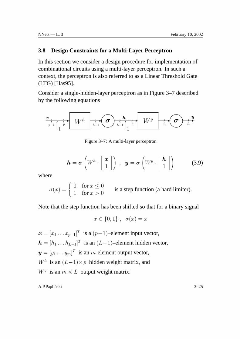
Consider a single-hidden-layer perceptron as in Figure 3–7 describedby the following equations

- W h -��σx o o

p−1 p�1

oL−1

ho oL−1 L

�1

- W y -��

-σo om m

y

Figure 3–7: A multi-layer perceptron

h = σ

W h · x

1

, y = σ

W y · h

1

(3.9)

where

σ(x) =

0 for x ≤ 01 for x > 0

is a step function (a hard limiter).

Note that the step function has been shifted so that for a binary signal

x ∈ {0, 1} , σ(x) = x

x = [x1 . . . xp−1]T is a(p−1)–element input vector,

h = [h1 . . . hL−1]T is an(L−1)–element hidden vector,

y = [y1 . . . ym]T is anm-element output vector,

W h is an(L−1)×p hidden weight matrix, and

W y is anm× L output weight matrix.



The input and hidden signals are augmented with constants:

xp = 1 , andhL = 1

The total number of adjustable weights is

nw = (L− 1)p + m · L = L(p + m)− p (3.10)

Design Procedure

Assume that we are given the set ofN points X

Y

=

x(1) . . . x(N)y(1) . . . y(N)

(3.11)

to be mapped by the perceptron so that

y(n) = f(x(n)) ∀n = 1, . . . , N. (3.12)

Combining eqns (3.9), (3.11), and (3.12) we obtain a set ofdesignconstraints (equations) which must be satisfied by the perceptron inorder for the required mapping to be achieved:

σ([

W y:,1:L−1 · σ

([W h

:,1:p−1 ·X]⊕c W h

:,p

)]⊕c W h

:,L

)= Y (3.13)

where

M ⊕c cdef= M + (1⊗ c)

describe addition of a column vectorc to every column of the matrixM (⊗ denotes the Kronecker product, and1 is a row vector of ones).Eqn (3.13) can be re-written as a set ofN individual constraints, onefor each output,y(n) wheren = 1, . . . N .

For a binary case, the eqn (3.11) represent a truth table ofm Booleanfunctions of(p− 1) variables. The size of this table is

N = 2p−1



The constraints (3.13) can now be simplify to[W y

:,1:L−1 · σ([

W h:,1:p−1 ·X

]⊕c W h

:,p

)]⊕c W h

:,L = Y (3.14)

Conjecture 1 Under appropriate assumptions the necessary conditionfor a solution to the design problem as in eqn (3.13) or (3.14) to existis that the number of weights must be greater that the of points to bemapped, that is,

L(p + m)− p > N

Hence, the number of hidden signals

L >N + p

p + m(3.15)

For a single output(m = 1) binary mapping whenN = 2p−1

eqn (3.15) becomes

L >2p−1 + p

p + 1(3.16)

Once the structural parametersp, L, m are known the weight matricesWh, Wy that satisfy the constraint equation (3.13), or (3.14) can beselected.



Example

Consider the XOR function for which

X

Y

=

0 1 0 10 0 1 1

1 1 1 0

, p = 3 , N = 2p−1 = 4 (3.17)

From eqn (3.16) we can estimate that

L >N + p

p + 1, Let L = 3

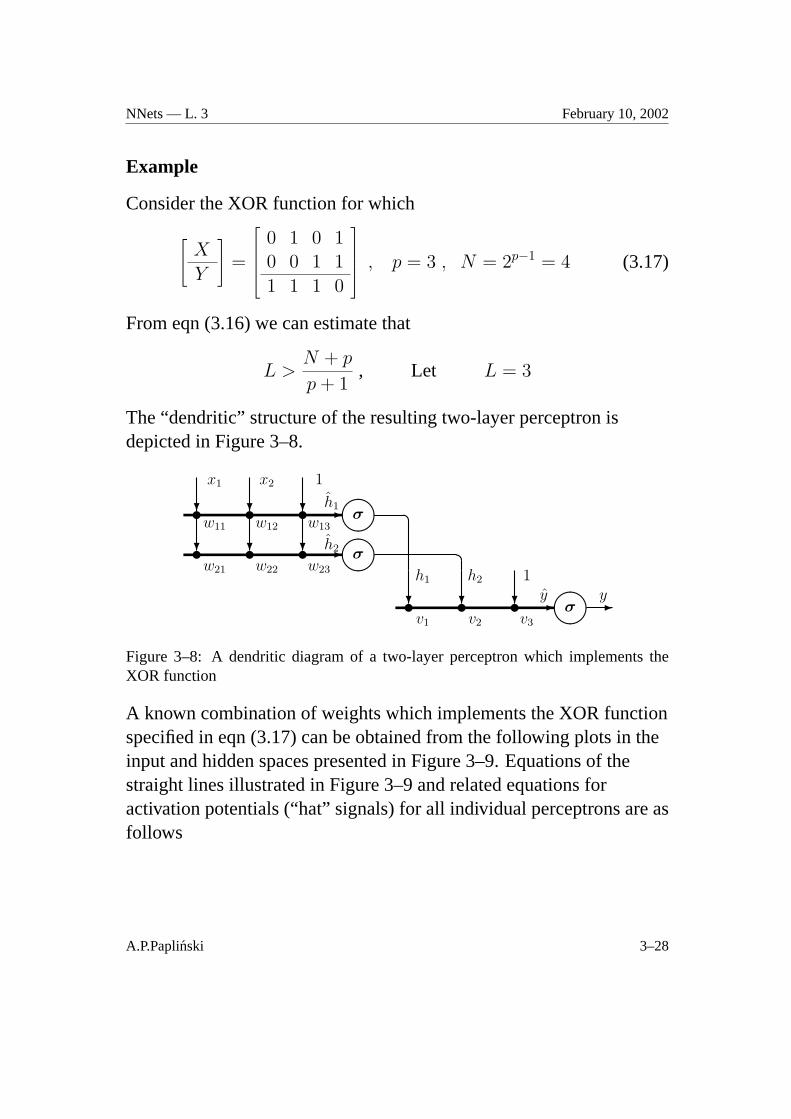
The “dendritic” structure of the resulting two-layer perceptron isdepicted in Figure 3–8.

��

σu u u? ? ? -

��

σu u u? ? ? -

x1 x2 1

w11 w12 w13

w21 w22 w23

h1

h2

��

σu u u? ? ? -

��

h1 h2 1

v1 v2 v3

-yy

Figure 3–8: A dendritic diagram of a two-layer perceptron which implements theXOR function

A known combination of weights which implements the XOR functionspecified in eqn (3.17) can be obtained from the following plots in theinput and hidden spaces presented in Figure 3–9. Equations of thestraight lines illustrated in Figure 3–9 and related equations foractivation potentials (“hat” signals) for all individual perceptrons are asfollows



-

6x2

x1

w1:

w2:

h2

h1

�

�4

4

·

·0

1

1

��

�@@

@@

@@

@@

@@

@@

@@

@@

@@

@@

@@

@@

-

6h2

h1

v

y

�

4·

0

1

1

��

@@

@@

@@

@@

@@

@@

� ⇒ y = 04 ⇒ y = 1

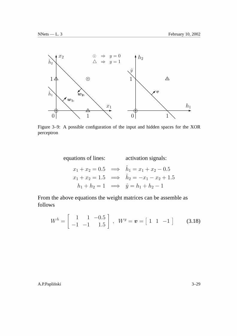
Figure 3–9: A possible configuration of the input and hidden spaces for the XORperceptron

equations of lines: activation signals:

x1 + x2 = 0.5 =⇒ h1 = x1 + x2 − 0.5

x1 + x2 = 1.5 =⇒ h2 = −x1 − x2 + 1.5

h1 + h2 = 1 =⇒ y = h1 + h2 − 1

From the above equations the weight matrices can be assemble asfollows

W h =

1 1 −0.5−1 −1 1.5

, W y = v =[

1 1 −1]

(3.18)



Constraint Equations for the XOR perceptron

In order to calculate other combinations of weights for the XORperceptron we can re-write the constraint equation (3.14) using thestructure as in Figure 3–8. The result is as follows

[v1 v2

]·σ

w11 w12

w21 w22

· 0 1 0 1

0 0 1 1

⊕c

w13

w23

+v3 =[

0 1 1 0]

(3.19)Eqn (3.19) is equivalent to the following four scalar equations, the totalnumber of weights to be selected being 9.

v1 · σ(w13) + v2 · σ(w23) + v3 = 0

v1 · σ(w11 + w13) + v2 · σ(w21 + w23) + v3 = 1

v1 · σ(w12 + w13) + v2 · σ(w22 + w23) + v3 = 1

v1 · σ(w11 + w12 + w13) + v2 · σ(w21 + w22 + w23) + v3 = 0

It can easily be verified that the weights specified in eqn (3.18) satisfythe above constraints.



References

[DB98] H. Demuth and M. Beale.Neural Network TOOLBOX User’s Guide. Foruse with MATLAB. The MathWorks Inc., 1998.

[FS91] J.A. Freeman and D.M. Skapura.Neural Networks. Algorithms,Applications, and Programming Techniques. Addison-Wesley, 1991.ISBN 0-201-51376-5.

[Has95] Mohamad H. Hassoun.Fundamentals of Artificial Neural Networks. TheMIT Press, 1995. ISBN 0-262-08239-X.

[Hay99] Simon Haykin.Neural Networks – a Comprehensive Foundation. PrenticeHall, New Jersey, 2nd edition, 1999. ISBN 0-13-273350-1.

[HDB96] Martin T. Hagan, H Demuth, and M. Beale.Neural Network Design. PWSPublishing, 1996.

[HKP91] Hertz, Krogh, and Palmer.Introduction to the Theory of NeuralComputation. Addison-Wesley, 1991. ISBN 0-201-51560-1.

[Kos92] Bart Kosko.Neural Networks for Signal Processing. Prentice-Hall, 1992.ISBN 0-13-617390-X.

[Sar98] W.S. Sarle, editor.Neural Network FAQ. Newsgroup: comp.ai.neural-nets,1998. URL: ftp://ftp.sas.com/pub/neural/FAQ.html.


neural network lecture 3

Documents

Transcript of neural network lecture 3