Optimisation of the B+ → K+π−π+γ selection at LHCb

Cyrille Praz

Master’s thesis

Directed by Prof. Dr. Olivier Schneider

Supervised by Dr. Preema Rennee Pais

22.06.2018

Abstract

The rare b → sγ radiative electroweak transition is a powerful probe of physics

beyond the Standard Model. This document presents a selection of B± → K±π∓π±γ

candidates in LHCb Run 2 data samples collected at a centre-of-mass energy of 13 TeV.

The selection uses a cut-based strategy followed by a multivariate analysis and a

characterisation of the signal and background sources. Approximately 3’000, 18’000

and 18’000 B± → K±π∓π±γ decays are selected in 2015, 2016 and 2017 data samples

corresponding to integrated luminosities of 0.29, 1.64 and 1.71 fb−1, respectively.

Contents

1 Introduction 3

2 Theoretical background 4

2.1 The Standard Model of particle physics . . . . . . . . . . . . . . . . . . . . 4

2.2 Radiative B decays in the Standard Model . . . . . . . . . . . . . . . . . . 6

2.3 Measurement of the photon polarisation parameter . . . . . . . . . . . . . . 7

3 The LHCb experiment 9

4 Optimisation of the B+ → K+π−π+γ selection 14

4.1 Data samples . . . . . . . . . . . . . . . . . . . . . . . . . . . . . . . . . . . 14

4.2 Stripping selection . . . . . . . . . . . . . . . . . . . . . . . . . . . . . . . . 14

4.3 Trigger lines . . . . . . . . . . . . . . . . . . . . . . . . . . . . . . . . . . . . 15

4.4 Cut-based strategy . . . . . . . . . . . . . . . . . . . . . . . . . . . . . . . . 16

4.5 Multivariate analysis . . . . . . . . . . . . . . . . . . . . . . . . . . . . . . . 23

4.5.1 XGBoost . . . . . . . . . . . . . . . . . . . . . . . . . . . . . . . . . 23

4.5.2 Training . . . . . . . . . . . . . . . . . . . . . . . . . . . . . . . . . . 26

4.5.3 Results and choice of the final cut . . . . . . . . . . . . . . . . . . . 28

5 Study of the B+ → K+π−π+γ signal 32

5.1 Signal study . . . . . . . . . . . . . . . . . . . . . . . . . . . . . . . . . . . . 32

5.2 Background study . . . . . . . . . . . . . . . . . . . . . . . . . . . . . . . . 32

5.2.1 Combinatorial background . . . . . . . . . . . . . . . . . . . . . . . . 33

5.2.2 Partially reconstructed b-hadron background . . . . . . . . . . . . . 33

5.2.3 Peaking backgrounds . . . . . . . . . . . . . . . . . . . . . . . . . . . 35

5.3 Mass fit . . . . . . . . . . . . . . . . . . . . . . . . . . . . . . . . . . . . . . 38

6 Conclusion and outlook 42

A Appendix 43

A.1 Uncertainty on efficiency . . . . . . . . . . . . . . . . . . . . . . . . . . . . . 43

A.2 Background coming from B+ → D0ρ+ decays . . . . . . . . . . . . . . . . . 44

A.3 2015 and 2017 data . . . . . . . . . . . . . . . . . . . . . . . . . . . . . . . . 45

2

1 Introduction

In the last decades, particle physics experiments involving hundreds or even thousands

of scientists have drastically improved our understanding of how Nature works. So far,

the vast majority of results obtained are compatible with the predictions of the Standard

Model of particle physics (SM), which describes with high precision the elementary par-

ticles and their fundamental interactions. However, one knows that the SM is not yet the

theory of everything. In particular, large scale phenomena such as gravity and dark matter

are not included in the SM. In the latter case, whereas many observations have already

provided evidence for the existence of dark matter [1–3], its nature remains unknown.

Many extensions of the SM have been developed, and one of the roles of experimental

particle physics is to test and constrain these new models. The photon polarisation in

the rare b → sγ transition is very sensitive to potential New Physics (NP) effects: in the

SM, this transition is not allowed at tree level and it implies that the photon is predicted

to be mostly left-handed, because the W boson appearing in the electroweak penguin

loop couples only to a left-handed s quark. New particles could appear at loop level and

enhance the right-handed component of the photon polarisation.

By studying the rare B+ → K+res(→ K+π−π+)γ decay, which has three pseudoscalar

mesons in its final state, one can access the polarisation of the photon by using its direction

with respect to the plane defined by the momenta of the three mesons in the rest frame

of the kaon resonance [4–6]. Several experimental studies of this decay have already been

conducted with data collected during the first run (Run 1) of the LHC [7–9] resulting in

the first observation of a non-zero photon polarisation [10].

This thesis documents the selection of B+ → K+π−π+γ candidates1 in data samples

collected with the LHCb detector at a centre-of-mass energy of 13 TeV in 2015, 2016 and

2017, corresponding to integrated luminosities of 0.29, 1.64 and 1.71 fb−1 respectively.

Section 2 gives a theoretical background, Sec. 3 describes briefly the main components

of the LHCb detector, Sec. 4 explains the cut-based and multivariate analysis strategies

used to select the signal decays and Sec. 5 presents a study of the signal and background

sources and the obtained results. Several strategies presented in this study are based on

what was done for Run 1 data [7–11].

1Unless explicitly stated otherwise, the charge-conjugate process is implied throughout this document.

3

2 Theoretical background

This section explains the theoretical motivation to measure the photon polarisation in the

rare b → sγ transition. Sections 2.1 and 2.2 present a quick overview of the Standard

Model of particle physics and its prediction about the photon polarisation, and Sec. 2.3

introduces two methods to investigate the photon polarisation.

2.1 The Standard Model of particle physics

The Standard Model of particle physics (SM) unifies in a single framework most of the

current knowledge that we have about the fundamental particles and their interactions.

As a relativistic quantum field theory, the SM is based on the symmetry group

SU(3)C ⊗ SU(2)L ⊗ U(1)YW , (1)

where C stands for the color charge, L the left chirality and YW the weak hypercharge.

SU(3)C is the symmetry group of the strong interaction, described by Quantum Chromo-

dynamics (QCD), whereas SU(2)L ⊗ U(1)YW is the symmetry group of the Electroweak

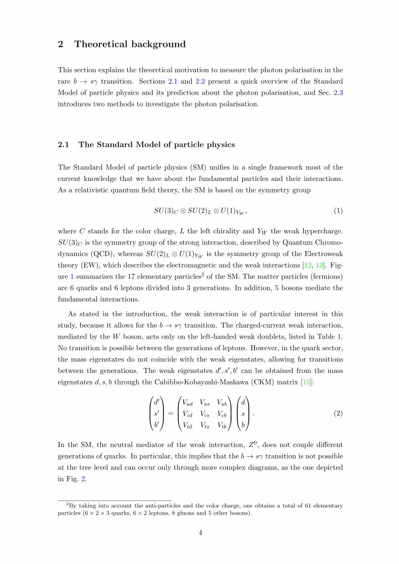
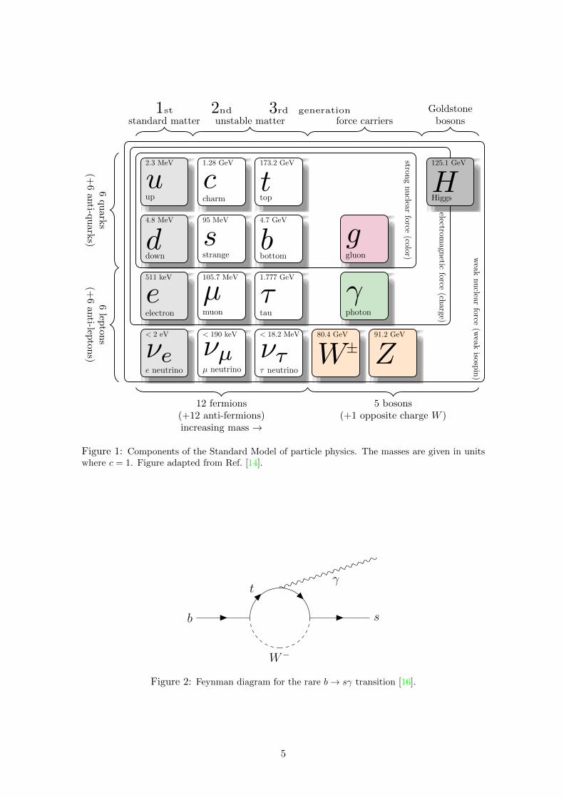
theory (EW), which describes the electromagnetic and the weak interactions [12, 13]. Fig-

ure 1 summarises the 17 elementary particles2 of the SM. The matter particles (fermions)

are 6 quarks and 6 leptons divided into 3 generations. In addition, 5 bosons mediate the

fundamental interactions.

As stated in the introduction, the weak interaction is of particular interest in this

study, because it allows for the b→ sγ transition. The charged-current weak interaction,

mediated by the W boson, acts only on the left-handed weak doublets, listed in Table 1.

No transition is possible between the generations of leptons. However, in the quark sector,

the mass eigenstates do not coincide with the weak eigenstates, allowing for transitions

between the generations. The weak eigenstates d′, s′, b′ can be obtained from the mass

eigenstates d, s, b through the Cabibbo-Kobayashi-Maskawa (CKM) matrix [15]:d′

s′

b′

=

Vud Vus Vub

Vcd Vcs Vcb

Vtd Vts Vtb

d

s

b

. (2)

In the SM, the neutral mediator of the weak interaction, Z0, does not couple different

generations of quarks. In particular, this implies that the b→ sγ transition is not possible

at the tree level and can occur only through more complex diagrams, as the one depicted

in Fig. 2.

2By taking into account the anti-particles and the color charge, one obtains a total of 61 elementaryparticles (6 × 2 × 3 quarks, 6 × 2 leptons, 8 gluons and 5 other bosons).

4

2.3 MeV

up

u4.8 MeV

downd511 keV

electron

e< 2 eV

e neutrino

νe

1.28 GeV

charm

c95 MeV

strange

s105.7 MeV

muon

µ< 190 keV

µ neutrino

νµ

173.2 GeV

topt4.7 GeV

bottomb1.777 GeV

tau

τ< 18.2 MeV

τ neutrino

ντ80.4 GeV

W±91.2 GeV

Z

photon

γ

gluon

g

125.1 GeV

HiggsH

strongnuclear

force(co

lor)

electromagnetic

force(ch

arge)

weak

nuclear

force(w

eakisosp

in)

6quarks

(+6an

ti-quarks)

6lep

tons

(+6anti-lep

tons)

12 fermions(+12 anti-fermions)increasing mass →

5 bosons(+1 opposite charge W )

standard matter unstable matter force carriersGoldstonebosons

1st 2nd 3rd generation

Figure 1: Components of the Standard Model of particle physics. The masses are given in unitswhere c = 1. Figure adapted from Ref. [14].

b s

W−

tγ

Figure 2: Feynman diagram for the rare b→ sγ transition [16].

5

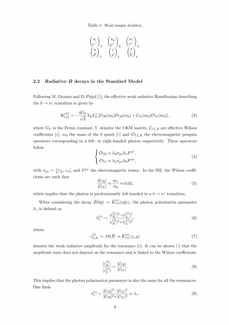
Table 1: Weak isospin doublets.

(νee−

)L

(νµµ−

)L

(νττ−

)L(

ud′

)L

(cs′

)L

(tb′

)L

2.2 Radiative B decays in the Standard Model

Following M. Gronau and D. Pirjol [5], the effective weak radiative Hamiltonian describing

the b→ sγ transition is given by

Heffrad = −4GF√2VtbV

∗ts [C7R(mb)O7R(mb) + C7L(mb)O7L(mb)] , (3)

where GF is the Fermi constant, V denotes the CKM matrix, C7L,R are effective Wilson

coefficients [6], mb the mass of the b quark [6] and O7L,R the electromagnetic penguin

operators corresponding to a left- or right-handed photon respectively. These operators

follow O7R ∝ sRσµνbLFµν ,O7L ∝ sLσµνbRFµν ,

(4)

with σµν = i2 [γµ, γν ], and Fµν the electromagnetic tensor. In the SM, the Wilson coeffi-

cients are such that|C7R||C7L|

≈ ms

mb≈ 0.02, (5)

which implies that the photon is predominantly left-handed in a b→ sγ transition.

When considering the decay B(bq) → K(i)res(sq)γ, the photon polarisation parameter

λγ is defined as

λ(i)γ :=

|c(i)R |2−|c

(i)L |2

|c(i)R |2+|c(i)

L |2, (6)

where

c(i)L,R :=M(B → K(i)

resγL,R) (7)

denotes the weak radiative amplitude for the resonance (i). It can be shown [5] that the

amplitude ratio does not depend on the resonance and is linked to the Wilson coefficients:

|c(i)R ||c(i)L |

=|C7R||C7L|

. (8)

This implies that the photon polarisation parameter is also the same for all the resonances.

One finds

λ(i)γ =

|C7R|2−|C7L|2|C7R|2+|C7L|2

≡ λγ . (9)

6

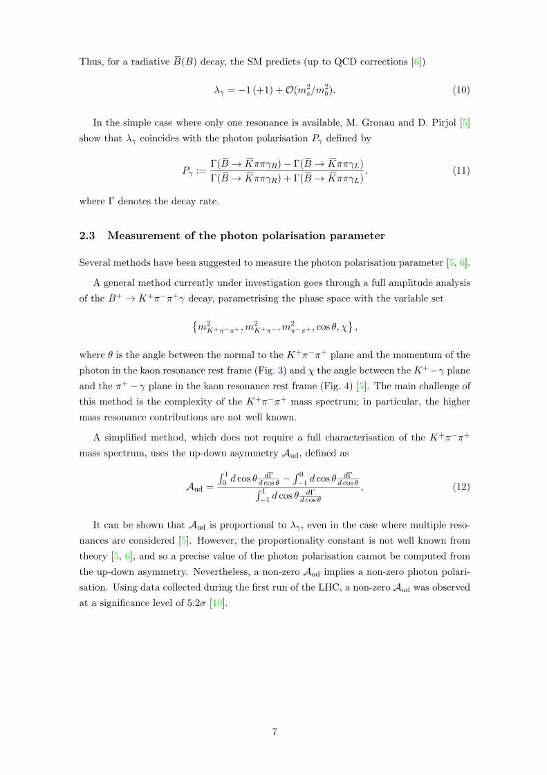
Thus, for a radiative B(B) decay, the SM predicts (up to QCD corrections [6])

λγ = −1 (+1) +O(m2s/m

2b). (10)

In the simple case where only one resonance is available, M. Gronau and D. Pirjol [5]

show that λγ coincides with the photon polarisation Pγ defined by

Pγ :=Γ(B → KππγR)− Γ(B → KππγL)

Γ(B → KππγR) + Γ(B → KππγL), (11)

where Γ denotes the decay rate.

2.3 Measurement of the photon polarisation parameter

Several methods have been suggested to measure the photon polarisation parameter [5, 6].

A general method currently under investigation goes through a full amplitude analysis

of the B+ → K+π−π+γ decay, parametrising the phase space with the variable set

{m2K+π−π+ ,m

2K+π− ,m

2π−π+ , cos θ, χ

},

where θ is the angle between the normal to the K+π−π+ plane and the momentum of the

photon in the kaon resonance rest frame (Fig. 3) and χ the angle between the K+−γ plane

and the π+− γ plane in the kaon resonance rest frame (Fig. 4) [5]. The main challenge of

this method is the complexity of the K+π−π+ mass spectrum; in particular, the higher

mass resonance contributions are not well known.

A simplified method, which does not require a full characterisation of the K+π−π+

mass spectrum, uses the up-down asymmetry Aud, defined as

Aud =

∫ 10 d cos θ dΓ

d cos θ −∫ 0−1 d cos θ dΓ

d cos θ∫ 1−1 d cos θ dΓ

d cos θ

, (12)

It can be shown that Aud is proportional to λγ , even in the case where multiple reso-

nances are considered [5]. However, the proportionality constant is not well known from

theory [5, 6], and so a precise value of the photon polarisation cannot be computed from

the up-down asymmetry. Nevertheless, a non-zero Aud implies a non-zero photon polari-

sation. Using data collected during the first run of the LHC, a non-zero Aud was observed

at a significance level of 5.2σ [10].

7

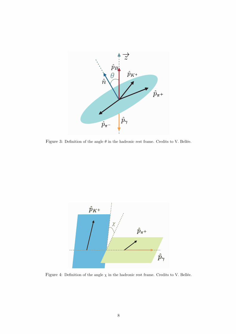
Figure 3: Definition of the angle θ in the hadronic rest frame. Credits to V. Bellee.

Figure 4: Definition of the angle χ in the hadronic rest frame. Credits to V. Bellee.

8

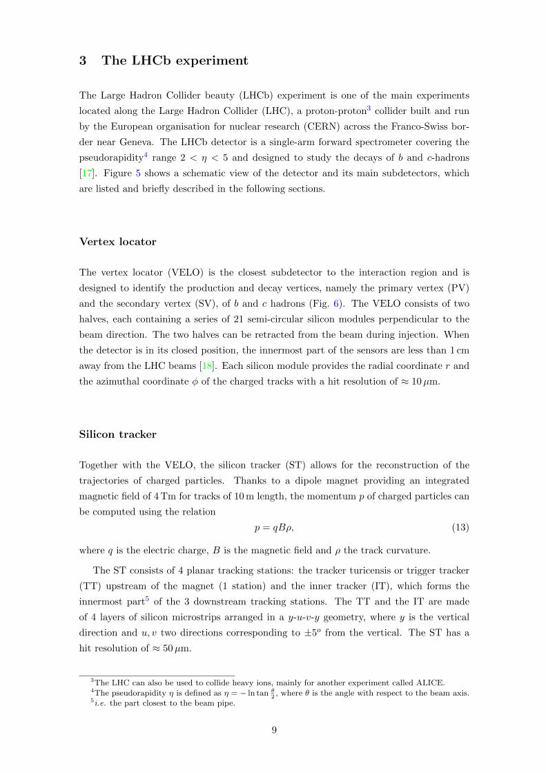
3 The LHCb experiment

The Large Hadron Collider beauty (LHCb) experiment is one of the main experiments

located along the Large Hadron Collider (LHC), a proton-proton3 collider built and run

by the European organisation for nuclear research (CERN) across the Franco-Swiss bor-

der near Geneva. The LHCb detector is a single-arm forward spectrometer covering the

pseudorapidity4 range 2 < η < 5 and designed to study the decays of b and c-hadrons

[17]. Figure 5 shows a schematic view of the detector and its main subdetectors, which

are listed and briefly described in the following sections.

Vertex locator

The vertex locator (VELO) is the closest subdetector to the interaction region and is

designed to identify the production and decay vertices, namely the primary vertex (PV)

and the secondary vertex (SV), of b and c hadrons (Fig. 6). The VELO consists of two

halves, each containing a series of 21 semi-circular silicon modules perpendicular to the

beam direction. The two halves can be retracted from the beam during injection. When

the detector is in its closed position, the innermost part of the sensors are less than 1 cm

away from the LHC beams [18]. Each silicon module provides the radial coordinate r and

the azimuthal coordinate φ of the charged tracks with a hit resolution of ≈ 10µm.

Silicon tracker

Together with the VELO, the silicon tracker (ST) allows for the reconstruction of the

trajectories of charged particles. Thanks to a dipole magnet providing an integrated

magnetic field of 4 Tm for tracks of 10 m length, the momentum p of charged particles can

be computed using the relation

p = qBρ, (13)

where q is the electric charge, B is the magnetic field and ρ the track curvature.

The ST consists of 4 planar tracking stations: the tracker turicensis or trigger tracker

(TT) upstream of the magnet (1 station) and the inner tracker (IT), which forms the

innermost part5 of the 3 downstream tracking stations. The TT and the IT are made

of 4 layers of silicon microstrips arranged in a y-u-v-y geometry, where y is the vertical

direction and u, v two directions corresponding to ±5o from the vertical. The ST has a

hit resolution of ≈ 50µm.

3The LHC can also be used to collide heavy ions, mainly for another experiment called ALICE.4The pseudorapidity η is defined as η = − ln tan θ

2, where θ is the angle with respect to the beam axis.

5i.e. the part closest to the beam pipe.

9

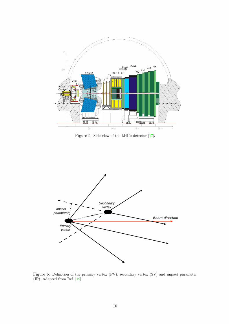
Figure 5: Side view of the LHCb detector [17].

Figure 6: Definition of the primary vertex (PV), secondary vertex (SV) and impact parameter(IP). Adapted from Ref. [19].

10

Outer tracker

The outer tracker (OT), which is a drift-time detector, forms the outside part of the

downstream tracking stations. Similarly to the ST, each of the 3 stations of the OT has

4 layers arranged in a y-u-v-y geometry. Each layer is made of 2 staggered sublayers of

drift-tubes filled with a mixture of Ar/CO2/O2 (70/28.5/1.5) [20]. Together with the IT,

the OT constitutes the 3 tracking stations T1, T2 and T3.

Ring-imaging Cherenkov detectors

Two ring-imaging Cherenkov counters (RICH1 and RICH2), upstream and downstream

of the magnet respectively, are used to identify charged particles. If a charged particle

travels through a medium of refraction index n faster than light in this medium, it emits

a light cone of angle θc related to its velocity β through

β =1

n cos θc. (14)

RICH1 uses a C4F10 radiator and covers the momentum range ≈ 1 − 60 GeV/c, while

RICH2 uses a CF4 radiator and covers the range ≈ 15 − 100 GeV/c. Both detectors

contain mirrors to reflect the Cherenkov light out of the LHCb acceptance. By combining

the information about momentum (Eq. 13) and velocity (Eq. 14), the mass of the particle

(its identity) follows from m = p/(γβ), where γ = 1/√

1− β2.

Calorimeters

The calorimeters give information about the identity, energy and position of the final

state electrons, photons and hadrons. They consist of an electromagnetic calorimeter

(ECAL) followed by a hadronic calorimeter (HCAL) of 25 and 5.6 radiation lengths re-

spectively. The ECAL (HCAL) has a scintillator/lead (scintillator/iron) sampling struc-

ture. The scintillating light produced by both calorimeters is transmitted to phototubes

by wavelength-shifting fibres.

The identification of electrons is challenging due to a high background of pions. Two

subdetectors in front of the ECAL are designed to reject this background: a scintillator

pad detector (SPD) and a preshower detector (PS). The SPD is used to separate electrons

from photons and neutral pions, and the PS segments the electromagnetic shower detection

for charged pions identification.

Muon system

The muon system is composed of 5 stations (M1−M5). M1 is located upstream of the

calorimeter and is based on a triple gas electron multiplier (GEM). M2−M5 are located

downstream of the calorimeter and use iron absorbers and multi-wire proportional cham-

11

bers (MWPC). M1−M3 have a high spatial resolution and provide a momentum resolution

of ≈ 20%, whereas M4−M5 have a lower spatial resolution and are mainly used to identify

penetrating particles.

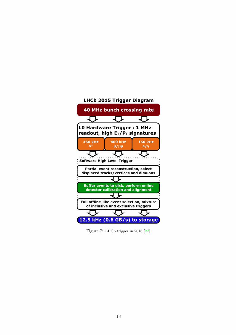
Trigger6

The LHCb trigger system is represented in Fig. 7. The LHC provides a bunch crossing

rate of 40 MHz, which is currently too high for the readout. The level-0 trigger (L0),

implemented in hardware, performs a first online selection based on the transverse mo-

mentum and energy of single particles (tracks or calorimeter clusters) and rejects also

high multiplicity events. After L0, two high level triggers (HLT1 and HLT2), consisting of

software algorithms, are used to achieve a final storage rate of 12.5 kHz in Run 2. HLT1

reconstructs tracks in events that pass the L0 stage and selects high quality tracks. The

event rate after HLT1 is low enough to buffer the events in a local disk. Thanks to this

buffer, an online calibration and alignment is executed before running the HLT2 on the

selected events. HLT2 reconstructs the full event and includes information on particle

identification.

6Because the trigger system was changed between Run 1 and Run 2, this section is based on Refs. [21, 22].

12

40 MHz bunch crossing rate

450 kHzh±

400 kHzµ/µµ

150 kHze/γ

L0 Hardware Trigger : 1 MHz readout, high ET/PT signatures

Software High Level Trigger

12.5 kHz (0.6 GB/s) to storage

Partial event reconstruction, select displaced tracks/vertices and dimuons

Buffer events to disk, perform online detector calibration and alignment

Full offline-like event selection, mixture of inclusive and exclusive triggers

LHCb 2015 Trigger Diagram

Figure 7: LHCb trigger in 2015 [22].

13

4 Optimisation of the B+ → K+π−π+γ selection

This section describes the selection of B+ → K+π−π+γ candidates in several data samples

collected with the LHCb detector. First, the data and Monte Carlo simulated samples con-

sidered are summarised (Sec. 4.1), the event preselection (stripping) is explained (Sec. 4.2)

and the trigger lines required are listed (Sec. 4.3). Then, a more precise background re-

jection strategy is developed: it consists of a set of cuts (Sec. 4.4) followed by the training

and application of a multivariate classifier (Sec. 4.5).

4.1 Data samples

The three data samples used in this study were collected with the LHCb detector at a

centre-of-mass energy of 13 TeV during the years 2015, 2016 and 2017. They correspond

to integrated recorded luminosities of 0.29, 1.64 and 1.71 fb−1, respectively. Monte Carlo

(MC) samples of signal and several sources of background are generated with Pythia8

[23] and fully simulated with Geant4 [24].

Table 2 lists the MC samples used, which are simulated using 2016 data-taking condi-

tions. The signal is simulated by the exclusive B+ → K1(1270)+γ decay, which is expected

to provide the highest contribution [10]. The other samples are used in Sec. 5 to model

several sources of background.

Based on the results of studies of the simulated signal sample (see Sec. 5.1), one intro-

duces three regions in the B mass distribution defined in Table 3: a signal region, and two

sidebands expected to contain mainly background.

4.2 Stripping selection

The first stage of the selection, called stripping, is a set of loose cuts aimed at preferentially

selecting events of interest to physics analyses. This is done during the central offline

processing of the data samples in order to save storage space and computational resources

[25]. The stripping configurations corresponding to 2015, 2016 and 2017 data considered

are S24, S28r1p1 and S29r2, respectively. Table 4 lists the main selection criteria applied

at this stage:

• The momentum p and transverse momentum pT of each track and the sum Σ pT

of all the transverse momenta coming from the resonance SV are required to be

large enough in order to reject low momentum background. For the same reason, a

minimum value is also imposed on the photon transverse energy ET and for the sum

of all the track transverse momenta and the photon transverse momentum.

• The χ2 of each track and each vertex is a measurement of the reconstruction quality.

It is near unity for a well-reconstructed track.

14

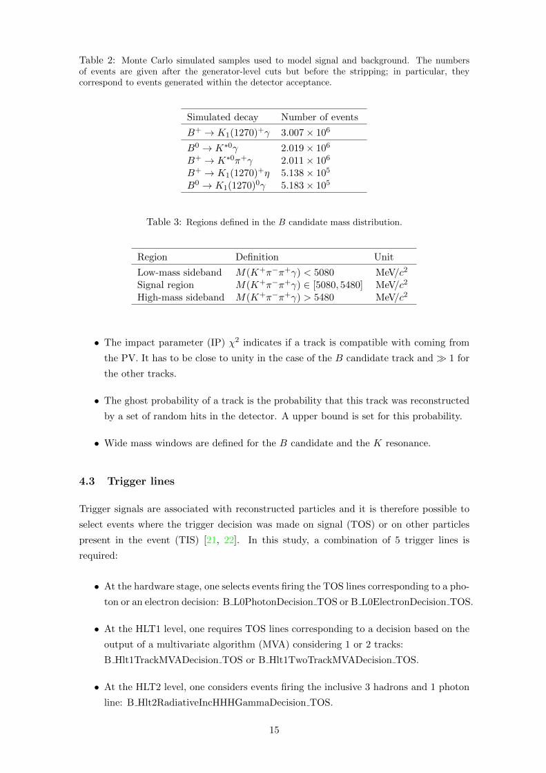
Table 2: Monte Carlo simulated samples used to model signal and background. The numbersof events are given after the generator-level cuts but before the stripping; in particular, theycorrespond to events generated within the detector acceptance.

Simulated decay Number of events

B+ → K1(1270)+γ 3.007× 106

B0 → K∗0γ 2.019× 106

B+ → K∗0π+γ 2.011× 106

B+ → K1(1270)+η 5.138× 105

B0 → K1(1270)0γ 5.183× 105

Table 3: Regions defined in the B candidate mass distribution.

Region Definition Unit

Low-mass sideband M(K+π−π+γ) < 5080 MeV/c2

Signal region M(K+π−π+γ) ∈ [5080, 5480] MeV/c2

High-mass sideband M(K+π−π+γ) > 5480 MeV/c2

• The impact parameter (IP) χ2 indicates if a track is compatible with coming from

the PV. It has to be close to unity in the case of the B candidate track and � 1 for

the other tracks.

• The ghost probability of a track is the probability that this track was reconstructed

by a set of random hits in the detector. A upper bound is set for this probability.

• Wide mass windows are defined for the B candidate and the K resonance.

4.3 Trigger lines

Trigger signals are associated with reconstructed particles and it is therefore possible to

select events where the trigger decision was made on signal (TOS) or on other particles

present in the event (TIS) [21, 22]. In this study, a combination of 5 trigger lines is

required:

• At the hardware stage, one selects events firing the TOS lines corresponding to a pho-

ton or an electron decision: B L0PhotonDecision TOS or B L0ElectronDecision TOS.

• At the HLT1 level, one requires TOS lines corresponding to a decision based on the

output of a multivariate algorithm (MVA) considering 1 or 2 tracks:

B Hlt1TrackMVADecision TOS or B Hlt1TwoTrackMVADecision TOS.

• At the HLT2 level, one considers events firing the inclusive 3 hadrons and 1 photon

line: B Hlt2RadiativeIncHHHGammaDecision TOS.

15

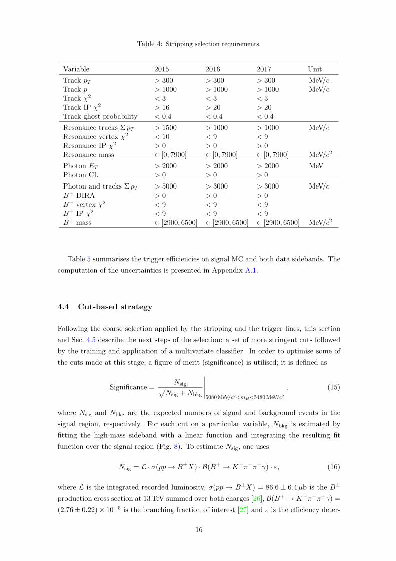
Table 4: Stripping selection requirements.

Variable 2015 2016 2017 Unit

Track pT > 300 > 300 > 300 MeV/cTrack p > 1000 > 1000 > 1000 MeV/cTrack χ2 < 3 < 3 < 3Track IP χ2 > 16 > 20 > 20Track ghost probability < 0.4 < 0.4 < 0.4

Resonance tracks Σ pT > 1500 > 1000 > 1000 MeV/cResonance vertex χ2 < 10 < 9 < 9Resonance IP χ2 > 0 > 0 > 0Resonance mass ∈ [0, 7900] ∈ [0, 7900] ∈ [0, 7900] MeV/c2

Photon ET > 2000 > 2000 > 2000 MeVPhoton CL > 0 > 0 > 0

Photon and tracks Σ pT > 5000 > 3000 > 3000 MeV/cB+ DIRA > 0 > 0 > 0B+ vertex χ2 < 9 < 9 < 9B+ IP χ2 < 9 < 9 < 9B+ mass ∈ [2900, 6500] ∈ [2900, 6500] ∈ [2900, 6500] MeV/c2

Table 5 summarises the trigger efficiencies on signal MC and both data sidebands. The

computation of the uncertainties is presented in Appendix A.1.

4.4 Cut-based strategy

Following the coarse selection applied by the stripping and the trigger lines, this section

and Sec. 4.5 describe the next steps of the selection: a set of more stringent cuts followed

by the training and application of a multivariate classifier. In order to optimise some of

the cuts made at this stage, a figure of merit (significance) is utilised; it is defined as

Significance =Nsig√

Nsig +Nbkg

∣∣∣∣∣5080 MeV/c2<mB<5480 MeV/c2

, (15)

where Nsig and Nbkg are the expected numbers of signal and background events in the

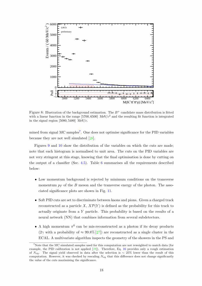
signal region, respectively. For each cut on a particular variable, Nbkg is estimated by

fitting the high-mass sideband with a linear function and integrating the resulting fit

function over the signal region (Fig. 8). To estimate Nsig, one uses

Nsig = L · σ(pp→ B±X) · B(B+ → K+π−π+γ) · ε, (16)

where L is the integrated recorded luminosity, σ(pp → B±X) = 86.6 ± 6.4µb is the B±

production cross section at 13 TeV summed over both charges [26], B(B+ → K+π−π+γ) =

(2.76± 0.22)× 10−5 is the branching fraction of interest [27] and ε is the efficiency deter-

16

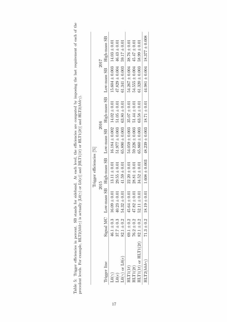
Tab

le5:

Tri

gger

effici

enci

esin

per

cent.

SB

stan

ds

for

sid

eban

d.

At

each

leve

l,th

eeffi

cien

cies

are

com

pu

ted

by

imp

osi

ng

the

last

requ

irem

ent

of

each

of

the

pre

ced

ent

leve

ls.

For

exam

ple

,H

LT

2(hhhγ

)is

actu

ally

[L0(γ

)or

L0(e

)]an

d[H

LT

1(1t)

or

HLT

1(2t)

]an

dH

LT

2(hhhγ

).

Tri

gger

effici

enci

es[%

]

2015

2016

2017

Tri

gger

lin

eS

ign

alM

CL

ow-m

ass

SB

Hig

h-m

ass

SB

Low

-mas

sS

BH

igh-m

ass

SB

Low

-mass

SB

Hig

h-m

ass

SB

L0(γ

)46.

1±

0.3

16.0

9±

0.0

113.1

1±

0.0

116.1

84±

0.0

0214.

02±

0.01

15.6

04±

0.003

14.

03±

0.0

1L

0(e)

37.7±

0.3

40.2

3±

0.0

129.5

5±

0.0

151.9

77±

0.0

0351.0

5±

0.01

47.8

29±

0.00

446.4

3±

0.0

1L

0(γ

)or

L0(e

)82.

1±

0.2

54.3

2±

0.0

141.5

9±

0.0

165.8

90±

0.0

0363.

80±

0.01

61.3

41±

0.003

59.

17±

0.0

1

HLT

1(1t)

69.1±

0.2

45.6

4±

0.0

122.2

0±

0.0

154.0

59±

0.0

0335.

07±

0.01

54.2

67±

0.004

38.

76±

0.0

1H

LT

1(2t

)76.2±

0.2

47.8

2±

0.0

128.8

1±

0.0

159.2

26±

0.0

0351.4

4±

0.01

54.5

55±

0.00

445.4

7±

0.0

1H

LT

1(1t)

orH

LT

1(2t)

82.

1±

0.2

52.1

1±

0.0

134.5

2±

0.0

165.8

60±

0.0

0363.

58±

0.01

61.3

20±

0.003

58.

99±

0.0

1

HLT

2(hhhγ

)71.3±

0.2

18.1

9±

0.0

11.6

08±

0.0

0348.2

39±

0.0

0318.

71±

0.01

44.9

81±

0.0

04

18.3

77±

0.0

08

17

0

1000

2000

3000

4000

5000

6000 )2E

vent

s / (

60

MeV

/c LHCb

preliminary

5000 5200 5400 5600 5800 6000 6200 6400

]2) [MeV/cγ+π−π+M(K

5−05

Pull

Figure 8: Illustration of the background estimation. The B+ candidate mass distribution is fittedwith a linear function in the range [5700, 6500] MeV/c2 and the resulting fit function is integratedin the signal region [5080, 5480] MeV/c.

mined from signal MC samples7. One does not optimise significance for the PID variables

because they are not well simulated [28].

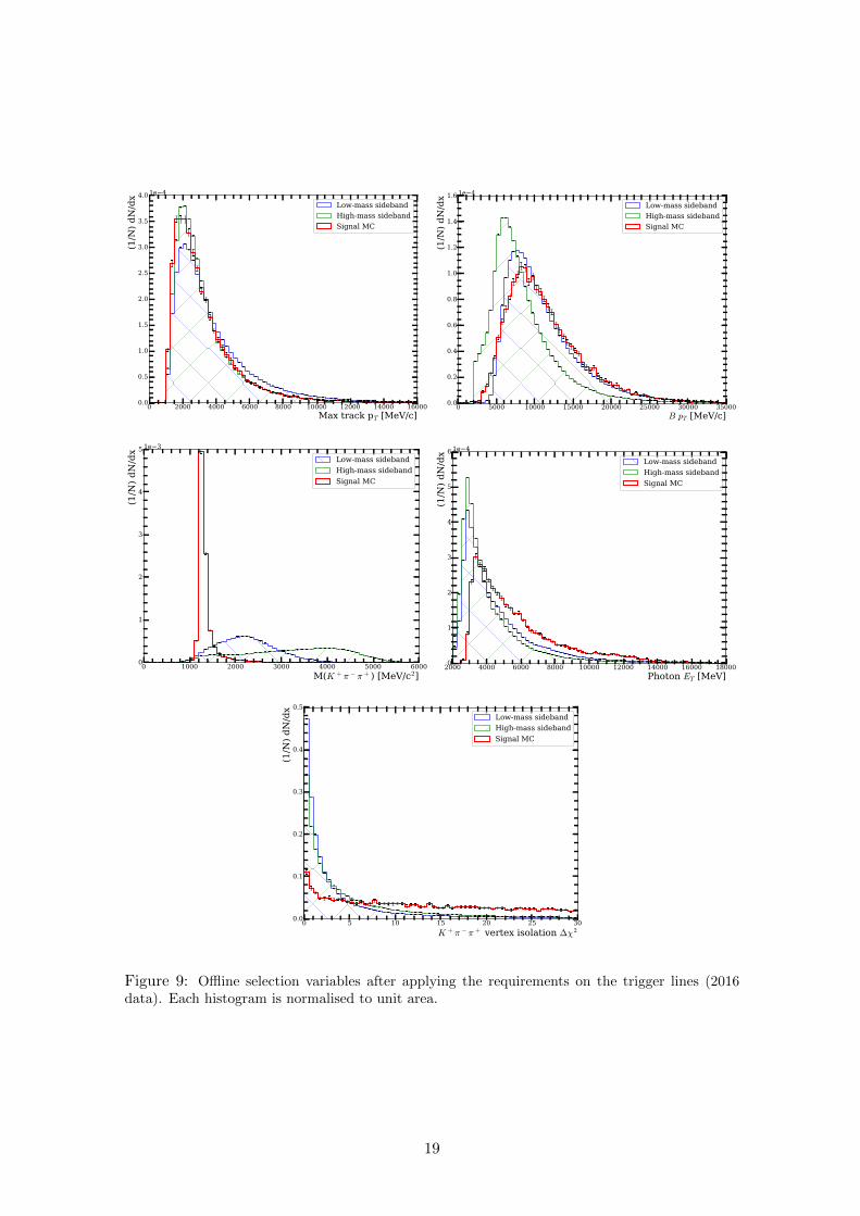
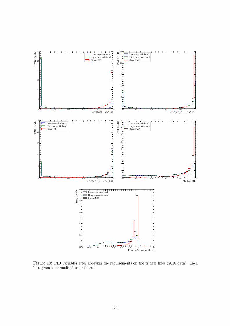
Figures 9 and 10 show the distribution of the variables on which the cuts are made;

note that each histogram is normalised to unit area. The cuts on the PID variables are

not very stringent at this stage, knowing that the final optimisation is done by cutting on

the output of a classifier (Sec. 4.5). Table 6 summarises all the requirements described

below:

• Low momentum background is rejected by minimum conditions on the transverse

momentum pT of the B meson and the transverse energy of the photon. The asso-

ciated significance plots are shown in Fig. 11.

• Soft PID cuts are set to discriminate between kaons and pions. Given a charged track

reconstructed as a particle X, XP(Y ) is defined as the probability for this track to

actually originate from a Y particle. This probability is based on the results of a

neural network (NN) that combines information from several subdetectors.

• A high momentum π0 can be mis-reconstructed as a photon if its decay products

(2γ with a probability of ≈ 99.8% [27]) are reconstructed as a single cluster in the

ECAL. A multivariate algorithm inspects the geometry of the showers in the PS and

7Note that the MC simulated samples used for this computation are not reweighted to match data (forexample, the PID calibration is not applied [28]). Therefore, Eq. 16 provides only a rough estimationof Nsig. The signal yield observed in data after the selection is ∼ 25% lower than the result of thiscomputation. However, it was checked by rescaling Nsig that this difference does not change significantlythe value of the cuts maximising the significance.

18

0 2000 4000 6000 8000 10000 12000 14000 16000

Max track pT [MeV/c]

0.0

0.5

1.0

1.5

2.0

2.5

3.0

3.5

4.0

(1/N

) d

N/d

x

1e 4

Low-mass sideband

High-mass sideband

Signal MC

0 5000 10000 15000 20000 25000 30000 35000

B pT [MeV/c]

0.0

0.2

0.4

0.6

0.8

1.0

1.2

1.4

1.6

(1/N

) d

N/d

x

1e 4

Low-mass sideband

High-mass sideband

Signal MC

0 1000 2000 3000 4000 5000 6000

M(K + π − π + ) [MeV/c2]

0

1

2

3

4

5

(1/N

) d

N/d

x

1e 3

Low-mass sideband

High-mass sideband

Signal MC

2000 4000 6000 8000 10000 12000 14000 16000 18000

Photon ET [MeV]

0

1

2

3

4

5

6

(1/N

) d

N/d

x1e 4

Low-mass sideband

High-mass sideband

Signal MC

0 5 10 15 20 25 30

K + π − π + vertex isolation ∆χ2

0.0

0.1

0.2

0.3

0.4

0.5

(1/N

) d

N/d

x

Low-mass sideband

High-mass sideband

Signal MC

Figure 9: Offline selection variables after applying the requirements on the trigger lines (2016data). Each histogram is normalised to unit area.

19

0.0 0.2 0.4 0.6 0.8 1.0

KP(K)(1−KP(π))

0

5

10

15

20

25

30

(1/N

) d

N/d

x

Low-mass sideband

High-mass sideband

Signal MC

0.0 0.2 0.4 0.6 0.8 1.0

π +P(π + )(1− π +P(K))

0

5

10

15

20

25

(1/N

) d

N/d

x

Low-mass sideband

High-mass sideband

Signal MC

0.0 0.2 0.4 0.6 0.8 1.0

π −P(π − )(1− π −P(K))

0

5

10

15

20

25

(1/N

) d

N/d

x

Low-mass sideband

High-mass sideband

Signal MC

0.0 0.2 0.4 0.6 0.8 1.0

Photon CL

0

2

4

6

8

10

12

14

16

(1/N

) d

N/d

x

Low-mass sideband

High-mass sideband

Signal MC

0.4 0.2 0.0 0.2 0.4 0.6 0.8 1.0 1.2 1.4

Photon/π0 separation

0

2

4

6

8

10

(1/N

) d

N/d

x

Low-mass sideband

High-mass sideband

Signal MC

Figure 10: PID variables after applying the requirements on the trigger lines (2016 data). Eachhistogram is normalised to unit area.

20

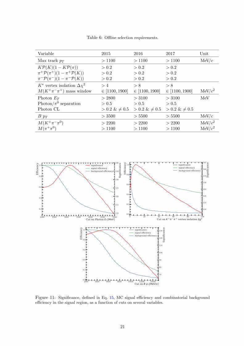
Table 6: Offline selection requirements.

Variable 2015 2016 2017 Unit

Max track pT > 1100 > 1100 > 1100 MeV/c

KP(K)(1−KP(π)) > 0.2 > 0.2 > 0.2π+P(π+)(1− π+P(K)) > 0.2 > 0.2 > 0.2π−P(π−)(1− π−P(K)) > 0.2 > 0.2 > 0.2

K∗ vertex isolation ∆χ2 > 4 > 8 > 8M(K+π−π+) mass window ∈ [1100, 1900] ∈ [1100, 1900] ∈ [1100, 1900] MeV/c2

Photon ET > 2800 > 3100 > 3100 MeVPhoton/π0 separation > 0.5 > 0.5 > 0.5Photon CL > 0.2 & 6= 0.5 > 0.2 & 6= 0.5 > 0.2 & 6= 0.5

B pT > 3500 > 5500 > 5500 MeV/c

M(K+π−π0) > 2200 > 2200 > 2200 MeV/c2

M(π+π0) > 1100 > 1100 > 1100 MeV/c2

2000 2500 3000 3500 4000 4500 5000Cut on Photon ET [MeV]

0.2

0.4

0.6

0.8

1.0

Eff

icie

ncy

110

115

120

125

130

135

140

Sign

ifica

nce

significancesignal efficiencybackground efficiency

0 20 40 60 80 100Cut on K + + vertex isolation 2

0.0

0.2

0.4

0.6

0.8

1.0

Eff

icie

ncy

110

115

120

125

130

135

140

145

Sign

ifica

nce

significancesignal efficiencybackground efficiency

2000 4000 6000 8000 10000 12000 14000Cut on B pT [MeV/c]

0.0

0.2

0.4

0.6

0.8

1.0

Eff

icie

ncy

70

80

90

100

110

120

130

Sign

ifica

nce

significancesignal efficiencybackground efficiency

Figure 11: Significance, defined in Eq. 15, MC signal efficiency and combinatorial backgroundefficiency in the signal region, as a function of cuts on several variables.

21

the ECAL to allow for a γ − π0 separation.

• A photon-electron distinction is made based on the photon confidence level (CL)

defined as

CL =tanh(γDLLγ−e) + 1

2, (17)

where γDLLγ−e is the difference, for a particle identified as a photon, of the log-

likelihoods (DLL) of the photon and the electron hypotheses. These log-likelihoods

are obtained from information from the calorimeters. The value γDLLγ−e = 0

corresponds to an error in the PID variable; for this reason, the condition CL 6= 0.5

is imposed.

• Partially reconstructed background can be suppressed by checking that combining

any new track with the reconstructed resonance vertex causes a drop in the vertex

quality. For this purpose, one defines the vertex isolation ∆χ2 as

∆χ2 = mintrack

χ2(reconstructed vertex + track)− χ2(reconstructed vertex), (18)

where the minimum is taken over all the tracks in the event not belonging to the

original reconstructed vertex. A significance plot for this variable is shown in Fig. 11.

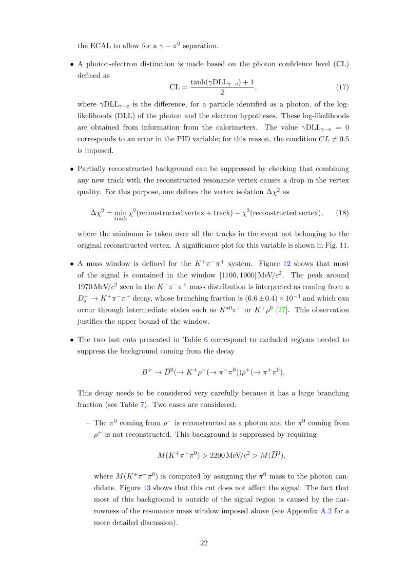
• A mass window is defined for the K+π−π+ system. Figure 12 shows that most

of the signal is contained in the window [1100, 1900] MeV/c2. The peak around

1970 MeV/c2 seen in the K+π−π+ mass distribution is interpreted as coming from a

D+s → K+π−π+ decay, whose branching fraction is (6.6±0.4)×10−3 and which can

occur through intermediate states such as K∗0π+ or K+ρ0 [27]. This observation

justifies the upper bound of the window.

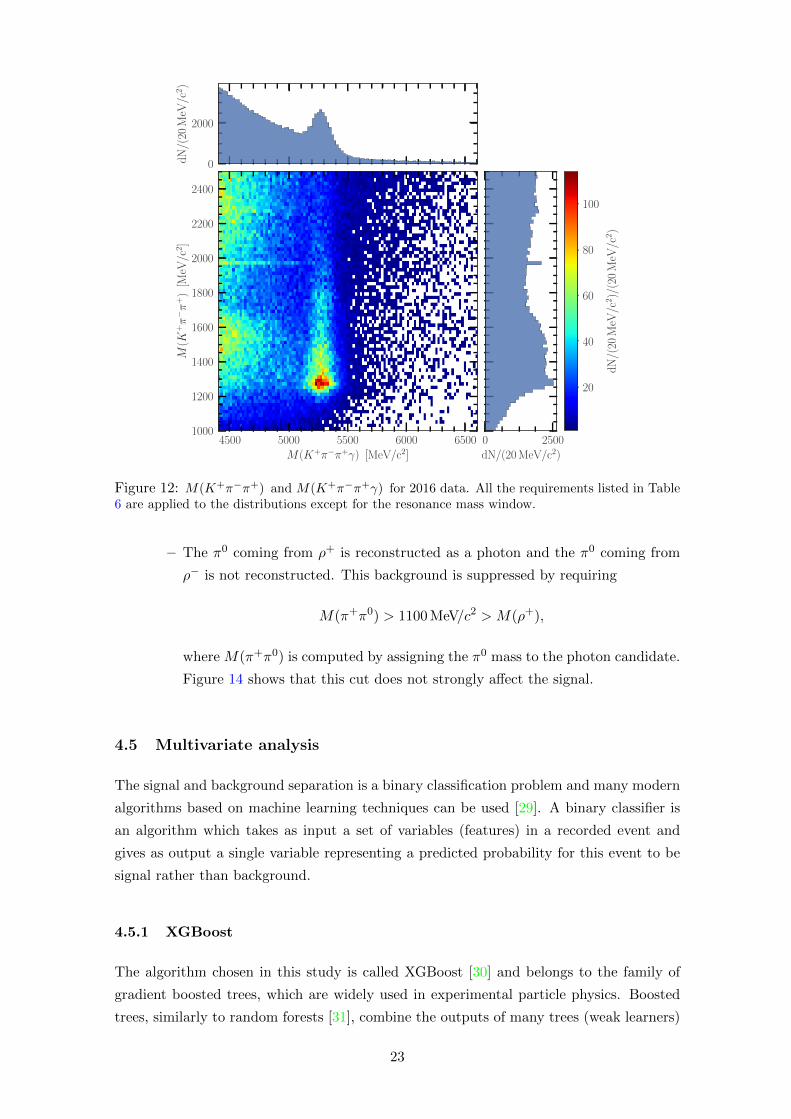
• The two last cuts presented in Table 6 correspond to excluded regions needed to

suppress the background coming from the decay

B+ → D0(→ K+ρ−(→ π−π0))ρ+(→ π+π0).

This decay needs to be considered very carefully because it has a large branching

fraction (see Table 7). Two cases are considered:

– The π0 coming from ρ− is reconstructed as a photon and the π0 coming from

ρ+ is not reconstructed. This background is suppressed by requiring

M(K+π−π0) > 2200 MeV/c2 > M(D0),

where M(K+π−π0) is computed by assigning the π0 mass to the photon can-

didate. Figure 13 shows that this cut does not affect the signal. The fact that

most of this background is outside of the signal region is caused by the nar-

rowness of the resonance mass window imposed above (see Appendix A.2 for a

more detailed discussion).

22

4500 5000 5500 6000 6500M(K+π−π+γ) [MeV/c2]

1000

1200

1400

1600

1800

2000

2200

2400M

(K+π−π

+)

[MeV

/c2]

0

2000

dN

/(20

MeV

/c2)

0 2500dN/(20 MeV/c2)

20

40

60

80

100

dN

/(20

MeV

/c2)/

(20

MeV

/c2)

Figure 12: M(K+π−π+) and M(K+π−π+γ) for 2016 data. All the requirements listed in Table6 are applied to the distributions except for the resonance mass window.

– The π0 coming from ρ+ is reconstructed as a photon and the π0 coming from

ρ− is not reconstructed. This background is suppressed by requiring

M(π+π0) > 1100 MeV/c2 > M(ρ+),

where M(π+π0) is computed by assigning the π0 mass to the photon candidate.

Figure 14 shows that this cut does not strongly affect the signal.

4.5 Multivariate analysis

The signal and background separation is a binary classification problem and many modern

algorithms based on machine learning techniques can be used [29]. A binary classifier is

an algorithm which takes as input a set of variables (features) in a recorded event and

gives as output a single variable representing a predicted probability for this event to be

signal rather than background.

4.5.1 XGBoost

The algorithm chosen in this study is called XGBoost [30] and belongs to the family of

gradient boosted trees, which are widely used in experimental particle physics. Boosted

trees, similarly to random forests [31], combine the outputs of many trees (weak learners)

23

3500 4000 4500 5000 5500 6000 6500M(K+π−π+γ) [MeV/c2]

1000

2000

3000

4000

5000

6000M

(K+π−π

0)

[MeV

/c2]

0

5000

dN

/(30

MeV

/c2)

0 5000dN/(30 MeV/c2)

100

200

300

400

500

dN

/(30

MeV

/c2)/

(30

MeV

/c2)

2016 Data

3500 4000 4500 5000 5500 6000 6500M(K+π−π+γ) [MeV/c2]

1000

2000

3000

4000

5000

6000

M(K

+π−π

0)

[MeV

/c2]

0

1000

2000

dN

/(30

MeV

/c2)

0 500dN/(30 MeV/c2)

10

20

30

40

50

60

70

80d

N/(

30M

eV/c

2)/

(30

MeV

/c2)

Signal MC

Figure 13: M(K+π−π0) and M(K+π−π+γ) for 2016 data (top) and signal MC (bottom), whereM(K+π−π0) is computed by assigning the π0 mass to the photon candidate. In data, the smallpeak around 1900 MeV/c2 corresponds to D0 (see text for details). All the requirements listed inTable 6 are applied to the distributions except for the two last ones.

24

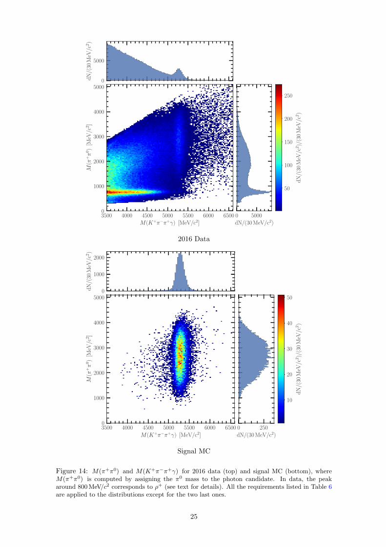
3500 4000 4500 5000 5500 6000 6500M(K+π−π+γ) [MeV/c2]

0

1000

2000

3000

4000

5000M

(π+π

0)

[MeV

/c2]

0

5000

dN

/(30

MeV

/c2)

0 5000dN/(30 MeV/c2)

50

100

150

200

250

dN

/(30

MeV

/c2)/

(30

MeV

/c2)

2016 Data

3500 4000 4500 5000 5500 6000 6500M(K+π−π+γ) [MeV/c2]

0

1000

2000

3000

4000

5000

M(π

+π

0)

[MeV

/c2]

0

1000

2000

dN

/(30

MeV

/c2)

0 250dN/(30 MeV/c2)

10

20

30

40

50d

N/(

30M

eV/c

2)/

(30

MeV

/c2)

Signal MC

Figure 14: M(π+π0) and M(K+π−π+γ) for 2016 data (top) and signal MC (bottom), whereM(π+π0) is computed by assigning the π0 mass to the photon candidate. In data, the peakaround 800 MeV/c2 corresponds to ρ+ (see text for details). All the requirements listed in Table 6are applied to the distributions except for the two last ones.

25

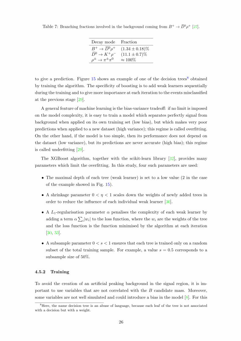
Table 7: Branching fractions involved in the background coming from B+ → D0ρ+ [27].

Decay mode Fraction

B+ → D0ρ+ (1.34± 0.18)%

D0 → K+ρ− (11.1± 0.7)%ρ± → π±π0 ≈ 100%

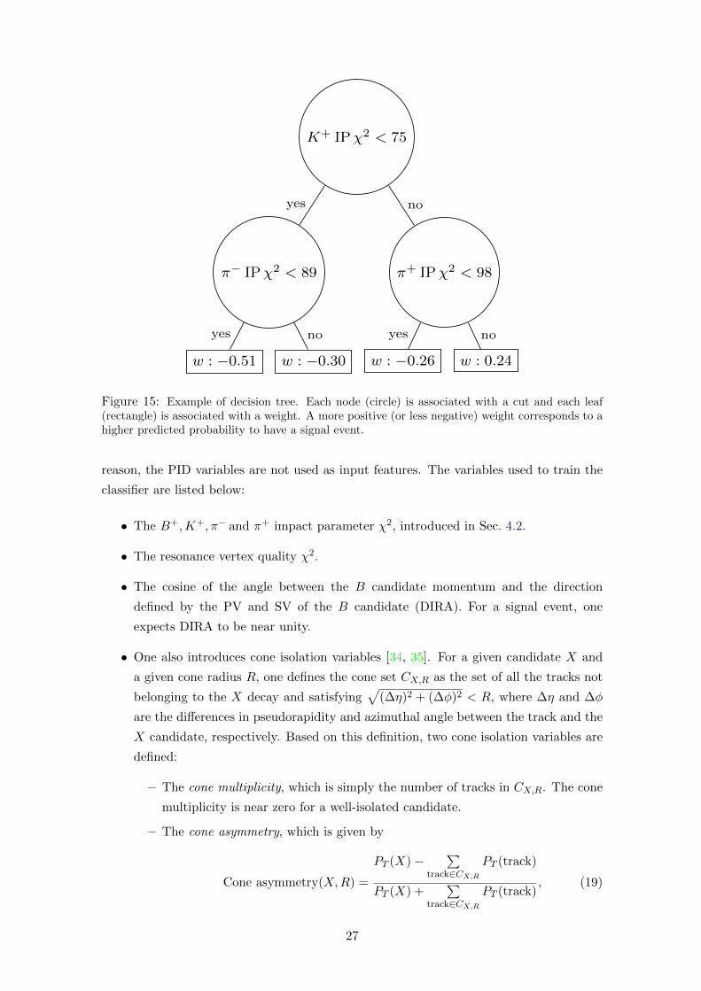
to give a prediction. Figure 15 shows an example of one of the decision trees8 obtained

by training the algorithm. The specificity of boosting is to add weak learners sequentially

during the training and to give more importance at each iteration to the events misclassified

at the previous stage [29].

A general feature of machine learning is the bias-variance tradeoff: if no limit is imposed

on the model complexity, it is easy to train a model which separates perfectly signal from

background when applied on its own training set (low bias), but which makes very poor

predictions when applied to a new dataset (high variance); this regime is called overfitting.

On the other hand, if the model is too simple, then its performance does not depend on

the dataset (low variance), but its predictions are never accurate (high bias); this regime

is called underfitting [29].

The XGBoost algorithm, together with the scikit-learn library [32], provides many

parameters which limit the overfitting. In this study, four such parameters are used:

• The maximal depth of each tree (weak learner) is set to a low value (2 in the case

of the example showed in Fig. 15).

• A shrinkage parameter 0 < η < 1 scales down the weights of newly added trees in

order to reduce the influence of each individual weak learner [30].

• A L1-regularisation parameter α penalises the complexity of each weak learner by

adding a term α∑

i|wi| to the loss function, where the wi are the weights of the tree

and the loss function is the function minimised by the algorithm at each iteration

[30, 33].

• A subsample parameter 0 < s < 1 ensures that each tree is trained only on a random

subset of the total training sample. For example, a value s = 0.5 corresponds to a

subsample size of 50%.

4.5.2 Training

To avoid the creation of an artificial peaking background in the signal region, it is im-

portant to use variables that are not correlated with the B candidate mass. Moreover,

some variables are not well simulated and could introduce a bias in the model [8]. For this

8Here, the name decision tree is an abuse of language, because each leaf of the tree is not associatedwith a decision but with a weight.

26

K+ IPχ2 < 75

π− IPχ2 < 89

w : −0.51 w : −0.30

π+ IPχ2 < 98

w : −0.26 w : 0.24

yes

yes no

no

yes no

Figure 15: Example of decision tree. Each node (circle) is associated with a cut and each leaf(rectangle) is associated with a weight. A more positive (or less negative) weight corresponds to ahigher predicted probability to have a signal event.

reason, the PID variables are not used as input features. The variables used to train the

classifier are listed below:

• The B+,K+, π− and π+ impact parameter χ2, introduced in Sec. 4.2.

• The resonance vertex quality χ2.

• The cosine of the angle between the B candidate momentum and the direction

defined by the PV and SV of the B candidate (DIRA). For a signal event, one

expects DIRA to be near unity.

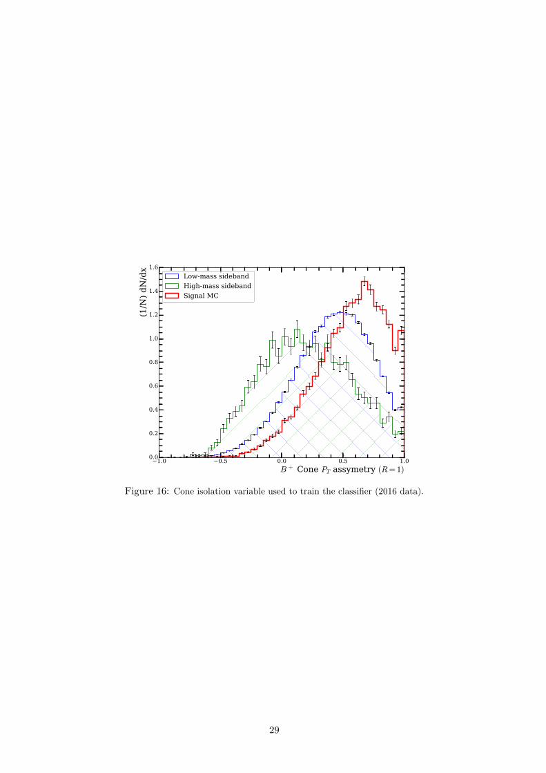
• One also introduces cone isolation variables [34, 35]. For a given candidate X and

a given cone radius R, one defines the cone set CX,R as the set of all the tracks not

belonging to the X decay and satisfying√

(∆η)2 + (∆φ)2 < R, where ∆η and ∆φ

are the differences in pseudorapidity and azimuthal angle between the track and the

X candidate, respectively. Based on this definition, two cone isolation variables are

defined:

– The cone multiplicity, which is simply the number of tracks in CX,R. The cone

multiplicity is near zero for a well-isolated candidate.

– The cone asymmetry, which is given by

Cone asymmetry(X,R) =

PT (X)− ∑track∈CX,R

PT (track)

PT (X) +∑

track∈CX,RPT (track)

, (19)

27

where PT (X) is the transverse momentum of X. The cone asymmetry is near

unity for a well-isolated candidate (Fig. 16).

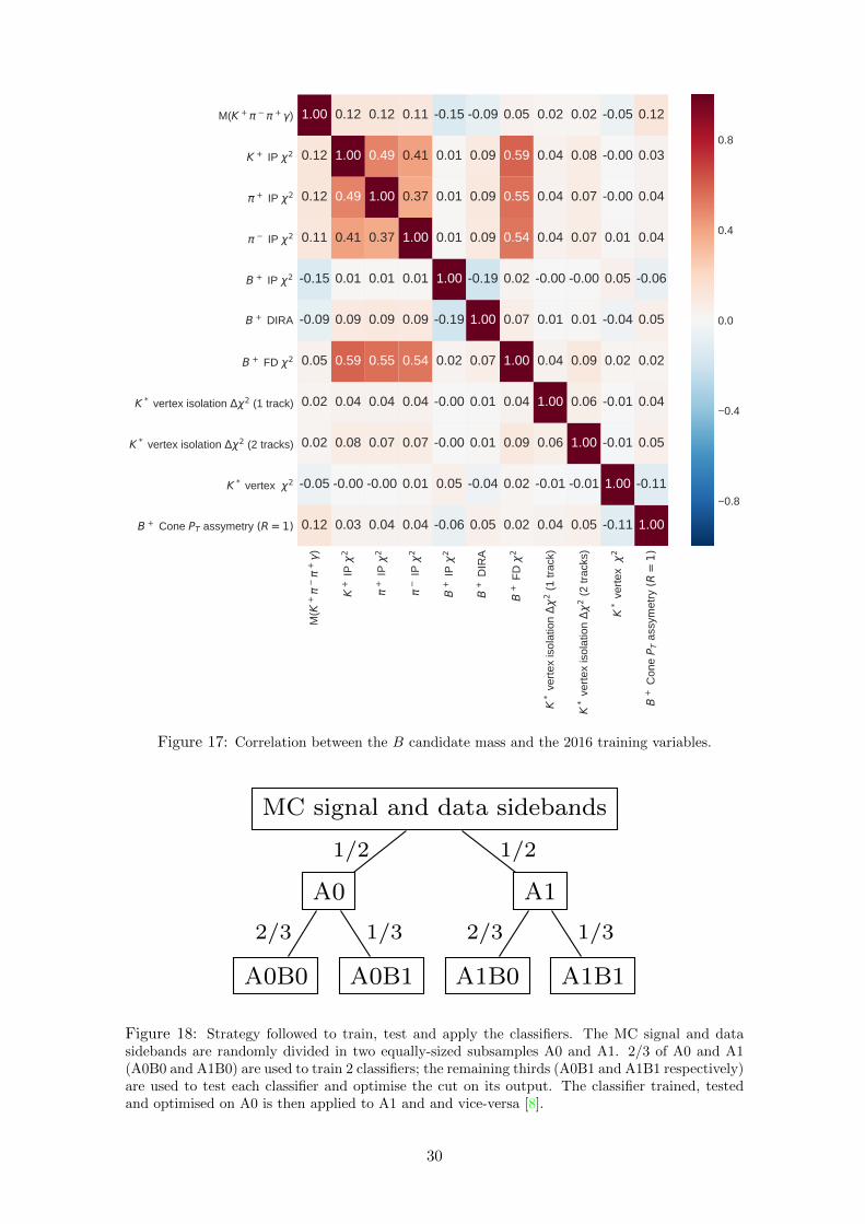
These variables have already shown a good discrimination power in a previous analysis of

Run 1 data [8]. Their correlation matrix with the B candidate mass is drawn in Fig. 17.

In order to ensure that the classifier is trained, optimised and applied on different

datasets, one follows the strategy depicted in Fig. 18 and inspired from Ref. [8]:

1. The MC signal and both data sidebands are randomly divided in two subsamples A0

and A1 of equal size and in such a manner that both subsamples contain the same

proportion of events coming from the MC signal and from the data sidebands.

2. A0 itself is divided in two subsamples, A0B0 and A0B1, of relative size 2/3 and

1/3 respectively. A0B0 is used to train a first classifier and the A0B1 subsample is

used to test it and optimise the cut on its output. Similarly, A1 is divided in two

subsamples A1B0 and A1B1 and a new classifier is trained, tested and optimised

following the same steps.

3. The classifier trained on A0B0 (A1B0) is applied to A1 (A0) in such a way that no

classifier is trained and applied on same data.

4.5.3 Results and choice of the final cut

Figure 19 shows the distribution of the output of the two classifiers and compares the

results obtained for the respective training set and test set together with the results of a

Kolmogorov-Smirnov test for an overfitting check [36]. The associated significance plots

are drawn in Fig. 20: the optimal cuts on the classifiers output are found to be 0.16

(0.14) for the classifer trained on A0B0 (A1B0). Whereas the classifiers show a good

separation power, the significance does not increase significantly because the signal is

already dominant in the [5080, 5480] MeV/c2 mass region thanks to the pre-selection criteria

applied. In order to choose the final cut, another figure of merit, the purity, is investigated;

it is defined as

Purity =Nsig

Nsig +Nbkg

∣∣∣∣5080 MeV/c2<mB<5480 MeV/c2

, (20)

where Nsig and Nbkg are the expected numbers of signal and background events in the

signal region. The purity is also depicted in Fig. 20; note that Nbkg is still estimated by

fitting the high-mass sideband, which means that the signal significance and purity are

only computed with respect to the combinatorial background. It can be seen that a better

purity can be achieved without affecting strongly the significance. The final cut is choosen

to be 0.2 for the two classifiers. Depending on the needs of future studies, a more stringent

cut may be imposed.

28

1.0 0.5 0.0 0.5 1.0

B + Cone PT assymetry (R= 1)

0.0

0.2

0.4

0.6

0.8

1.0

1.2

1.4

1.6

(1/N

) d

N/d

x

Low-mass sideband

High-mass sideband

Signal MC

Figure 16: Cone isolation variable used to train the classifier (2016 data).

29

M(K

++

)

K+

 IP 

2

+ IP

 2

 IP 

2

B+

 IP 

2

B+

 DIR

A

B+

 FD

 2

K*  

vert

ex is

olat

ion 

2  (1

 trac

k)

K*  

vert

ex is

olat

ion 

2  (2

 trac

ks)

K*  

vert

ex  

2

B+

 Con

e P T

 ass

ymet

ry (R

=1)

B +  Cone PT assymetry (R = 1)

K *  vertex   2

K *  vertex isolation  2 (2 tracks)

K *  vertex isolation  2 (1 track)

B +  FD  2

B +  DIRA

B +  IP  2

 IP  2

+  IP  2

K +  IP  2

M(K + + )

0.12 0.03 0.04 0.04 ­0.06 0.05 0.02 0.04 0.05 ­0.11 1.00

­0.05 ­0.00 ­0.00 0.01 0.05 ­0.04 0.02 ­0.01 ­0.01 1.00 ­0.11

0.02 0.08 0.07 0.07 ­0.00 0.01 0.09 0.06 1.00 ­0.01 0.05

0.02 0.04 0.04 0.04 ­0.00 0.01 0.04 1.00 0.06 ­0.01 0.04

0.05 0.59 0.55 0.54 0.02 0.07 1.00 0.04 0.09 0.02 0.02

­0.09 0.09 0.09 0.09 ­0.19 1.00 0.07 0.01 0.01 ­0.04 0.05

­0.15 0.01 0.01 0.01 1.00 ­0.19 0.02 ­0.00 ­0.00 0.05 ­0.06

0.11 0.41 0.37 1.00 0.01 0.09 0.54 0.04 0.07 0.01 0.04

0.12 0.49 1.00 0.37 0.01 0.09 0.55 0.04 0.07 ­0.00 0.04

0.12 1.00 0.49 0.41 0.01 0.09 0.59 0.04 0.08 ­0.00 0.03

1.00 0.12 0.12 0.11 ­0.15 ­0.09 0.05 0.02 0.02 ­0.05 0.12

0.8

0.4

0.0

0.4

0.8

Figure 17: Correlation between the B candidate mass and the 2016 training variables.

MC signal and data sidebands

A0

A0B0 A0B1

A1

A1B0 A1B1

1/2

2/3 1/3

1/2

2/3 1/3

Figure 18: Strategy followed to train, test and apply the classifiers. The MC signal and datasidebands are randomly divided in two equally-sized subsamples A0 and A1. 2/3 of A0 and A1(A0B0 and A1B0) are used to train 2 classifiers; the remaining thirds (A0B1 and A1B1 respectively)are used to test each classifier and optimise the cut on its output. The classifier trained, testedand optimised on A0 is then applied to A1 and and vice-versa [8].

30

0.0 0.2 0.4 0.6 0.8 1.0Classifier output

0.0

0.5

1.0

1.5

2.0

2.5

3.0

3.5

4.0

(1/N

) dN

/dx

Kolmogorov-Smirnov test: signal (background) p-value = 0.464 (0.352)Signal (test)Background (test)

Signal (training)Background (training)

0.0 0.2 0.4 0.6 0.8 1.0Classifier output

0.0

0.5

1.0

1.5

2.0

2.5

3.0

3.5

4.0

(1/N

) dN

/dx

Kolmogorov-Smirnov test: signal (background) p-value = 0.134 (0.267)Signal (test)Background (test)

Signal (training)Background (training)

Figure 19: Distribution of two classifiers outputs and comparison between the results obtainedwith the training and test sets. The first classifier (left) is trained on A0B0 and tested on A0B1;the second classifier (right) is trained on A1B0 and tested on A1B1.

0.0 0.2 0.4 0.6 0.8 1.0Cut on classifier output

0.0

0.2

0.4

0.6

0.8

1.0

Eff

icie

ncy

(Pur

ity)

0

20

40

60

80

100

120

Sign

ifica

nce

significancesignal efficiencybackground efficiencypurity

0.0 0.2 0.4 0.6 0.8 1.0Cut on classifier output

0.0

0.2

0.4

0.6

0.8

1.0

Eff

icie

ncy

(Pur

ity)

0

20

40

60

80

100

120

Sign

ifica

nce

significancesignal efficiencybackground efficiencypurity

Figure 20: Significance, purity, signal efficiency and background efficiency as a function of the cuton the two classifier outputs. The first classifier (left) is trained on A0B0 and tested on A0B1; thesecond classifier (right) is trained on A1B0 and tested on A1B1.

31

5 Study of the B+ → K+π−π+γ signal

In this section, the different components present in the B candidate mass distribution

after the selection are discussed and modelled (Secs. 5.1 and 5.2); this aims to build a full

mass fit (Sec. 5.3). All the fits presented are made with the RooFit package [37, 38].

5.1 Signal study

The signal is modelled with a double-tail Crystal Ball function (CB) [38, 39] defined as

CB(m; µ, σ, αL, nL, αR, nR) =

N

(nLαL

)nLexp

(−α2

L2

)(nLαL− αL − m−µ

σ

)−nLif m−µ

σ ≤ −αL,

exp(− (m−µ)2

2σ2

)if − αL < m−µ

σ < αR,(nRαR

)nRexp

(−α2

R2

)(nRαR− αR + m−µ

σ

)−nRif m−µ

σ ≥ αR,

(21)

where N is a normalisation constant and {µ, σ, αL, nL, αR, nR} is a set of 6 positive pa-

rameters described in Table 8. Out of these 6 parameters, only the mean µ and the width

σ are left free in the final fit; all the other parameters are fixed by fitting the B mass

distribution in the signal MC after applying the selection cuts presented in Sec. 4. Figure

21 presents the result of such a fit.

Based on the results of this simulation, one introduces three regions in the B mass

distribution defined in Table 3 and described below:

• The signal region is chosen to correspond approximately to the mean of the distri-

bution ±2σ.

• The high-mass sideband is expected to contain mainly combinatorial background,

which occurs when the reconstructed candidate contains random tracks coming from

an interaction point or from another decay chain.

• The low-mass sideband contains combinatorial and partially reconstructed back-

ground, the latter corresponding to b-hadron decays with more final state particles

than B+ → K+π−π+γ, but where one or several particles are not reconstructed.

5.2 Background study

As stated in the previous section, two main background components are still present after

the selection [8]: the combinatorial and the partially reconstructed backgrounds. In the

following paragraphs, these two sources of background and the possible combination of

them are discussed and modelled.

32

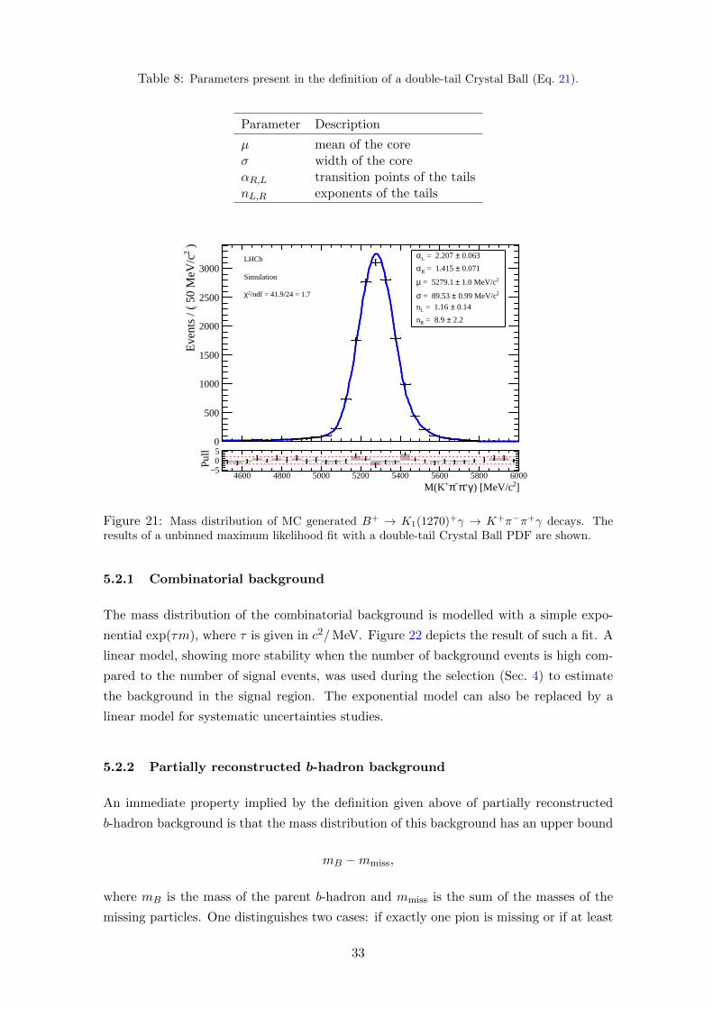
Table 8: Parameters present in the definition of a double-tail Crystal Ball (Eq. 21).

Parameter Description

µ mean of the coreσ width of the coreαR,L transition points of the tailsnL,R exponents of the tails

0

500

1000

1500

2000

2500

3000

)2E

vent

s / (

50

MeV

/c 0.063± = 2.207 Lα 0.071± = 1.415 Rα

2 1.0 MeV/c± = 5279.1 µ2 0.99 MeV/c± = 89.53 σ

0.14± = 1.16 Ln

2.2± = 8.9 Rn

LHCb

Simulation

/ndf = 41.9/24 = 1.72χ

4600 4800 5000 5200 5400 5600 5800 6000

]2) [MeV/cγ+π−π+M(K

5−05

Pull

Figure 21: Mass distribution of MC generated B+ → K1(1270)+γ → K+π−π+γ decays. Theresults of a unbinned maximum likelihood fit with a double-tail Crystal Ball PDF are shown.

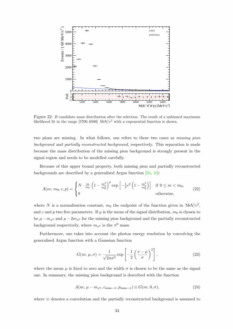
5.2.1 Combinatorial background

The mass distribution of the combinatorial background is modelled with a simple expo-

nential exp(τm), where τ is given in c2/MeV. Figure 22 depicts the result of such a fit. A

linear model, showing more stability when the number of background events is high com-

pared to the number of signal events, was used during the selection (Sec. 4) to estimate

the background in the signal region. The exponential model can also be replaced by a

linear model for systematic uncertainties studies.

5.2.2 Partially reconstructed b-hadron background

An immediate property implied by the definition given above of partially reconstructed

b-hadron background is that the mass distribution of this background has an upper bound

mB −mmiss,

where mB is the mass of the parent b-hadron and mmiss is the sum of the masses of the

missing particles. One distinguishes two cases: if exactly one pion is missing or if at least

33

0

1000

2000

3000

4000

5000

)2E

vent

s / (

60

MeV

/c LHCb

preliminary

5200 5400 5600 5800 6000 6200 6400

]2) [MeV/cγ+π−π+M(K

5−05

Pull

Figure 22: B candidate mass distribution after the selection. The result of a unbinned maximumlikelihood fit in the range [5700, 6500] MeV/c2 with a exponential function is shown.

two pions are missing. In what follows, one refers to these two cases as missing pion

background and partially reconstructed background, respectively. This separation is made

because the mass distribution of the missing pion background is strongly present in the

signal region and needs to be modelled carefully.

Because of this upper bound property, both missing pion and partially reconstructed

backgrounds are described by a generalised Argus function [38, 40]:

A(m; m0, c, p) =

N ·mm0

(1− m2

m20

)pexp

[−1

2c2(

1− m2

m20

)]if 0 ≤ m < m0,

0 otherwise,(22)

where N is a normalisation constant, m0 the endpoint of the function given in MeV/c2,

and c and p two free parameters. If µ is the mean of the signal distribution, m0 is chosen to

be µ−mπ0 and µ−2mπ0 for the missing pion background and the partially reconstructed

background respectively, where mπ0 is the π0 mass.

Furthermore, one takes into account the photon energy resolution by convolving the

generalised Argus function with a Gaussian function

G(m; µ, σ) =1√

2πσ2exp

[−1

2

(x− µσ

)2], (23)

where the mean µ is fixed to zero and the width σ is chosen to be the same as the signal

one. In summary, the missing pion background is described with the function

A(m; µ−mπ0 , cmiss−π, pmiss−π)⊗G(m; 0, σ), (24)

where ⊗ denotes a convolution and the partially reconstructed background is assumed to

34

follow the law

A(m; µ− 2mπ0 , cpart, ppart)⊗G(m; 0, σ). (25)

Single missing pion background

The missing pion background parameters cmiss−π and pmiss−π are fixed by simulation.

Due to the lack of B+ → K+π−π+π0γ MC samples, one uses simulated B0 → K∗0γ

and B+ → K∗0π+γ decays by analogy. A 3-step method is used to parametrise this

background contribution [8]:

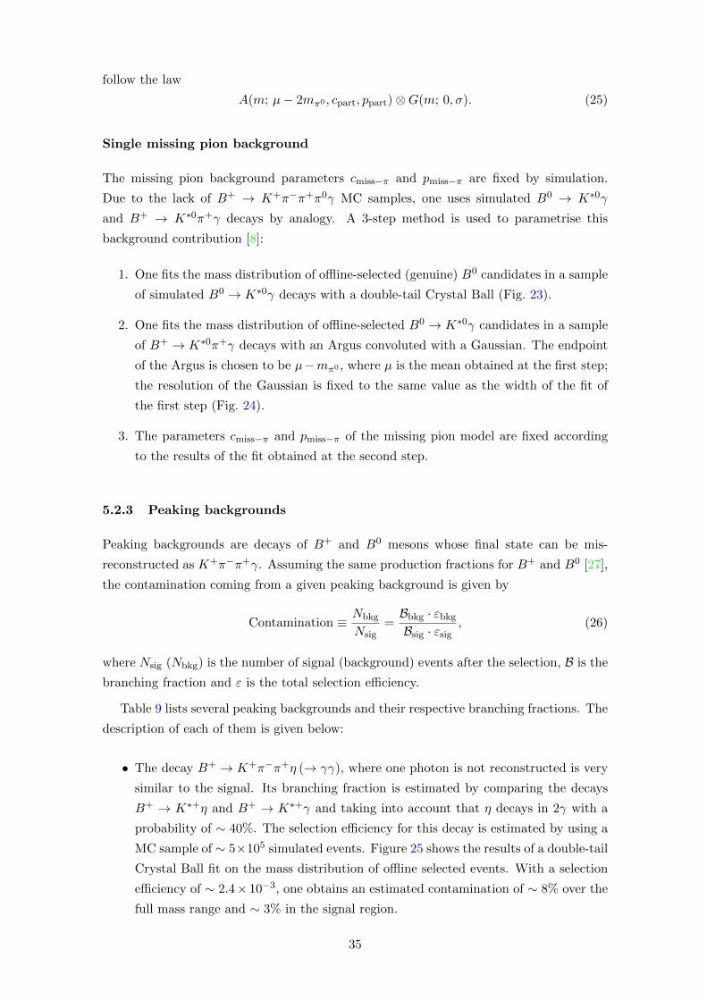
1. One fits the mass distribution of offline-selected (genuine) B0 candidates in a sample

of simulated B0 → K∗0γ decays with a double-tail Crystal Ball (Fig. 23).

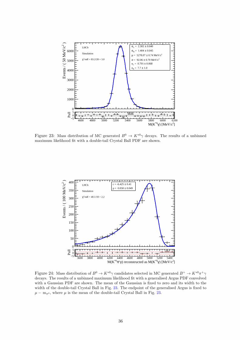
2. One fits the mass distribution of offline-selected B0 → K∗0γ candidates in a sample

of B+ → K∗0π+γ decays with an Argus convoluted with a Gaussian. The endpoint

of the Argus is chosen to be µ−mπ0 , where µ is the mean obtained at the first step;

the resolution of the Gaussian is fixed to the same value as the width of the fit of

the first step (Fig. 24).

3. The parameters cmiss−π and pmiss−π of the missing pion model are fixed according

to the results of the fit obtained at the second step.

5.2.3 Peaking backgrounds

Peaking backgrounds are decays of B+ and B0 mesons whose final state can be mis-

reconstructed as K+π−π+γ. Assuming the same production fractions for B+ and B0 [27],

the contamination coming from a given peaking background is given by

Contamination ≡ Nbkg

Nsig=Bbkg · εbkg

Bsig · εsig, (26)

where Nsig (Nbkg) is the number of signal (background) events after the selection, B is the

branching fraction and ε is the total selection efficiency.

Table 9 lists several peaking backgrounds and their respective branching fractions. The

description of each of them is given below:

• The decay B+ → K+π−π+η (→ γγ), where one photon is not reconstructed is very

similar to the signal. Its branching fraction is estimated by comparing the decays

B+ → K∗+η and B+ → K∗+γ and taking into account that η decays in 2γ with a

probability of ∼ 40%. The selection efficiency for this decay is estimated by using a

MC sample of ∼ 5×105 simulated events. Figure 25 shows the results of a double-tail

Crystal Ball fit on the mass distribution of offline selected events. With a selection

efficiency of ∼ 2.4× 10−3, one obtains an estimated contamination of ∼ 8% over the

full mass range and ∼ 3% in the signal region.

35

0

1000

2000

3000

4000

5000

6000

)2E

vent

s / (

50

MeV

/c 0.040± = 2.302 Lα 0.045± = 1.404 Rα

2 0.74 MeV/c± = 5278.07 µ2 0.70 MeV/c± = 92.06 σ

0.068± = 0.701 Ln

1.0± = 7.7 Rn

LHCb

Simulation

/ndf = 83.2/28 = 3.02χ

4600 4800 5000 5200 5400 5600 5800 6000 6200

]2) [MeV/cγ*0M(K

5−05

Pull

Figure 23: Mass distribution of MC generated B0 → K∗0γ decays. The results of a unbinnedmaximum likelihood fit with a double-tail Crystal Ball PDF are shown.

0

50

100

150

200

250

300

350

400 )2E

vent

s / (

100

MeV

/c 0.41±c = -6.425

0.049±p = 0.058 LHCb

Simulation

/ndf = 40.1/18 = 2.22χ

3600 3800 4000 4200 4400 4600 4800 5000 5200 5400

]2) [MeV/cγ*0) reconstructed as M(Kγ+π*0M(K

5−05

Pull

Figure 24: Mass distribution of B0 → K∗0γ candidates selected in MC generated B+ → K∗0π+γdecays. The results of a unbinned maximum likelihood fit with a generalised Argus PDF convolvedwith a Gaussian PDF are shown. The mean of the Gaussian is fixed to zero and its width to thewidth of the double-tail Crystal Ball in Fig. 23. The endpoint of the generalised Argus is fixed toµ− mπ0 , where µ is the mean of the double-tail Crystal Ball in Fig. 23.

36

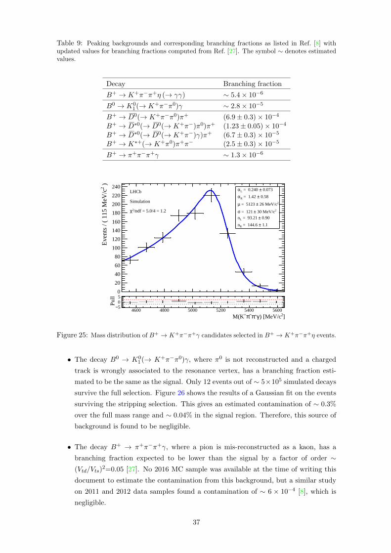
Table 9: Peaking backgrounds and corresponding branching fractions as listed in Ref. [8] withupdated values for branching fractions computed from Ref. [27]. The symbol ∼ denotes estimatedvalues.

Decay Branching fraction

B+ → K+π−π+η (→ γγ) ∼ 5.4× 10−6

B0 → K01 (→ K+π−π0)γ ∼ 2.8× 10−5

B+ → D0(→ K+π−π0)π+ (6.9± 0.3)× 10−4

B+ → D∗0(→ D0(→ K+π−)π0)π+ (1.23± 0.05)× 10−4

B+ → D∗0(→ D0(→ K+π−)γ)π+ (6.7± 0.3)× 10−5

B+ → K∗+(→ K+π0)π+π− (2.5± 0.3)× 10−5

B+ → π+π−π+γ ∼ 1.3× 10−6

0

20

40

60

80

100

120

140

160

180

200

220

240 )2E

vent

s / (

115

MeV

/c 0.073± = 0.240 Lα 0.58± = 1.42 Rα

2 26 MeV/c± = 5123 µ2 30 MeV/c± = 121 σ

0.90± = 93.21 Ln

1.1± = 144.6 Rn

LHCb

Simulation

/ndf = 5.0/4 = 1.22χ

4600 4800 5000 5200 5400 5600

]2) [MeV/cγ+π−π+M(K

5−05

Pull

Figure 25: Mass distribution of B+ → K+π−π+γ candidates selected in B+ → K+π−π+η events.

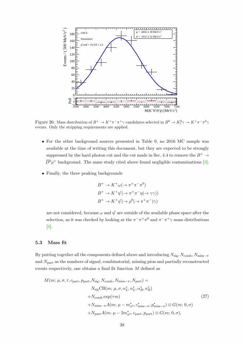
• The decay B0 → K01 (→ K+π−π0)γ, where π0 is not reconstructed and a charged

track is wrongly associated to the resonance vertex, has a branching fraction esti-

mated to be the same as the signal. Only 12 events out of ∼ 5×105 simulated decays

survive the full selection. Figure 26 shows the results of a Gaussian fit on the events

surviving the stripping selection. This gives an estimated contamination of ∼ 0.3%

over the full mass range and ∼ 0.04% in the signal region. Therefore, this source of

background is found to be negligible.

• The decay B+ → π+π−π+γ, where a pion is mis-reconstructed as a kaon, has a

branching fraction expected to be lower than the signal by a factor of order ∼(Vtd/Vts)

2=0.05 [27]. No 2016 MC sample was available at the time of writing this

document to estimate the contamination from this background, but a similar study

on 2011 and 2012 data samples found a contamination of ∼ 6 × 10−4 [8], which is

negligible.

37

0

20

40

60

80

100

120

140

160

180

)2E

vent

s / (

500

MeV

/c

2 38 MeV/c± = 4656 µ2 32 MeV/c± = 1031 σ

LHCb

Simulation

/ndf = 19.5/8 = 2.42χ

2500 3000 3500 4000 4500 5000 5500 6000 6500 7000 7500

]2) [MeV/cγ+π−π+M(K

5−05

Pull

Figure 26: Mass distribution of B+ → K+π−π+γ candidates selected in B0 → K01γ → K+π−π0γ

events. Only the stripping requirements are applied.

• For the other background sources presented in Table 9, no 2016 MC sample was

available at the time of writing this document, but they are expected to be strongly

suppressed by the hard photon cut and the cut made in Sec. 4.4 to remove the B+ →D0ρ+ background. The same study cited above found negligible contaminations [8].

• Finally, the three peaking backgrounds

B+ → K+ω(→ π+π−π0)

B+ → K+η′(→ π+π−η(→ γγ))

B+ → K+η′(→ ρ0(→ π+π−)γ)

are not considered, because ω and η′ are outside of the available phase space after the

selection, as it was checked by looking at the π−π+π0 and π−π+γ mass distributions

[8].

5.3 Mass fit

By putting together all the components defined above and introducing Nsig, Ncomb, Nmiss−πand Npart as the numbers of signal, combinatorial, missing pion and partially reconstructed

events respectively, one obtains a final fit function M defined as

M(m; µ, σ, τ, cpart, ppart,Nsig, Ncomb, Nmiss−π, Npart) =

NsigCB(m; µ, σ, α∗L, n∗L, α

∗R, n

∗R)

+Ncomb exp(τm)

+Nmiss−πA(m; µ−m∗π0 , c∗miss−π, p

∗miss−π)⊗G(m; 0, σ)

+NpartA(m; µ− 2m∗π0 , cpart, ppart)⊗G(m; 0, σ),

(27)

38

where the stars (*) denote fixed parameters listed in Table 11, whose values are determined

in Secs. 5.1 and 5.2.2.

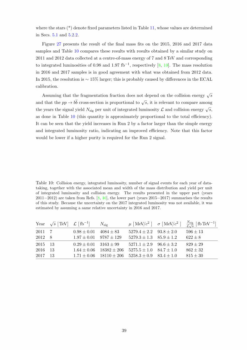
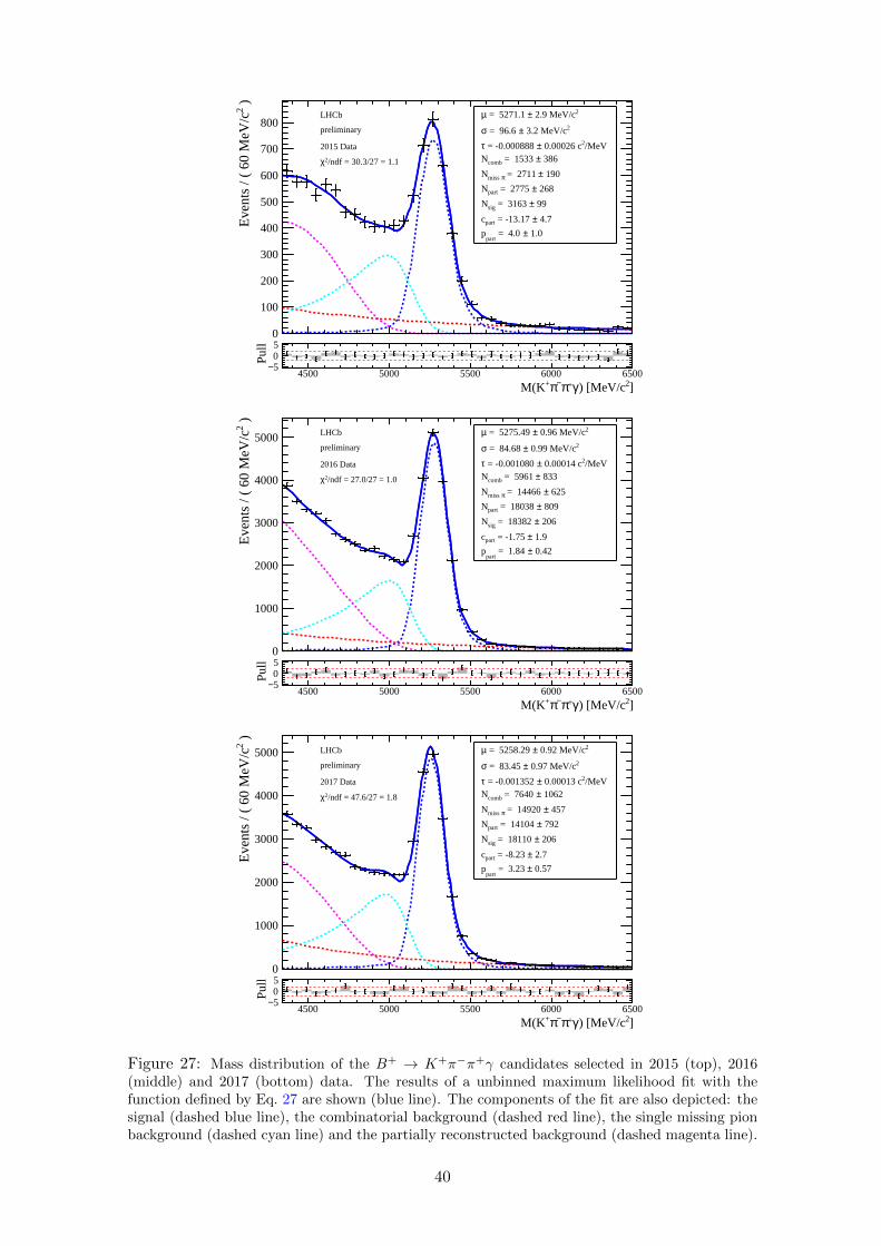
Figure 27 presents the result of the final mass fits on the 2015, 2016 and 2017 data

samples and Table 10 compares these results with results obtained by a similar study on

2011 and 2012 data collected at a centre-of-mass energy of 7 and 8 TeV and corresponding

to integrated luminosities of 0.98 and 1.97 fb−1, respectively [8, 10]. The mass resolution

in 2016 and 2017 samples is in good agreement with what was obtained from 2012 data.

In 2015, the resolution is ∼ 15% larger; this is probably caused by differences in the ECAL

calibration.

Assuming that the fragmentation fraction does not depend on the collision energy√s

and that the pp→ bb cross-section is proportional to√s, it is relevant to compare among

the years the signal yield Nsig per unit of integrated luminosity L and collision energy√s,

as done in Table 10 (this quantity is approximately proportional to the total efficiency).

It can be seen that the yield increases in Run 2 by a factor larger than the simple energy

and integrated luminosity ratio, indicating an improved efficiency. Note that this factor

would be lower if a higher purity is required for the Run 2 signal.

Table 10: Collision energy, integrated luminosity, number of signal events for each year of data-taking, together with the associated mean and width of the mass distribution and yield per unitof integrated luminosity and collision energy. The results presented in the upper part (years2011−2012) are taken from Refs. [8, 10], the lower part (years 2015−2017) summarises the resultsof this study. Because the uncertainty on the 2017 integrated luminosity was not available, it wasestimated by assuming a same relative uncertainty in 2016 and 2017.

Year√s [ TeV] L [ fb−1] Nsig µ [ MeV/c2 ] σ [ MeV/c2 ]

Nsig

L√s [ fb TeV−1]

2011 7 0.98± 0.01 4084± 83 5279.4± 2.2 93.8± 2.0 596± 132012 8 1.97± 0.01 9787± 129 5279.3± 1.3 85.9± 1.2 622± 8

2015 13 0.29± 0.01 3163± 99 5271.1± 2.9 96.6± 3.2 829± 292016 13 1.64± 0.06 18382± 206 5275.5± 1.0 84.7± 1.0 862± 322017 13 1.71± 0.06 18110± 206 5258.3± 0.9 83.4± 1.0 815± 30

39

0

100

200

300

400

500

600

700

800

)2E

vent

s / (

60

MeV

/c

2 2.9 MeV/c± = 5271.1 µ2 3.2 MeV/c± = 96.6 σ

/MeV2 0.00026 c± = -0.000888 τ 386± = 1533 combN

190± = 2711 πmiss N

268± = 2775 partN

99± = 3163 sigN

4.7± = -13.17 partc

1.0± = 4.0 part

p

LHCb

preliminary

2015 Data

/ndf = 30.3/27 = 1.12χ

4500 5000 5500 6000 6500

]2) [MeV/cγ+π−π+M(K

5−05

Pull

0

1000

2000

3000

4000

5000

)2E

vent

s / (

60

MeV

/c

2 0.96 MeV/c± = 5275.49 µ2 0.99 MeV/c± = 84.68 σ

/MeV2 0.00014 c± = -0.001080 τ 833± = 5961 combN

625± = 14466 πmiss N

809± = 18038 partN

206± = 18382 sigN

1.9± = -1.75 partc

0.42± = 1.84 part

p

LHCb

preliminary

2016 Data

/ndf = 27.0/27 = 1.02χ

4500 5000 5500 6000 6500

]2) [MeV/cγ+π−π+M(K

5−05

Pull

0

1000

2000

3000

4000

5000

)2E

vent

s / (

60

MeV

/c

2 0.92 MeV/c± = 5258.29 µ2 0.97 MeV/c± = 83.45 σ

/MeV2 0.00013 c± = -0.001352 τ 1062± = 7640 combN

457± = 14920 πmiss N

792± = 14104 partN

206± = 18110 sigN

2.7± = -8.23 partc

0.57± = 3.23 part

p

LHCb

preliminary

2017 Data

/ndf = 47.6/27 = 1.82χ

4500 5000 5500 6000 6500

]2) [MeV/cγ+π−π+M(K

5−05

Pull

Figure 27: Mass distribution of the B+ → K+π−π+γ candidates selected in 2015 (top), 2016(middle) and 2017 (bottom) data. The results of a unbinned maximum likelihood fit with thefunction defined by Eq. 27 are shown (blue line). The components of the fit are also depicted: thesignal (dashed blue line), the combinatorial background (dashed red line), the single missing pionbackground (dashed cyan line) and the partially reconstructed background (dashed magenta line).

40

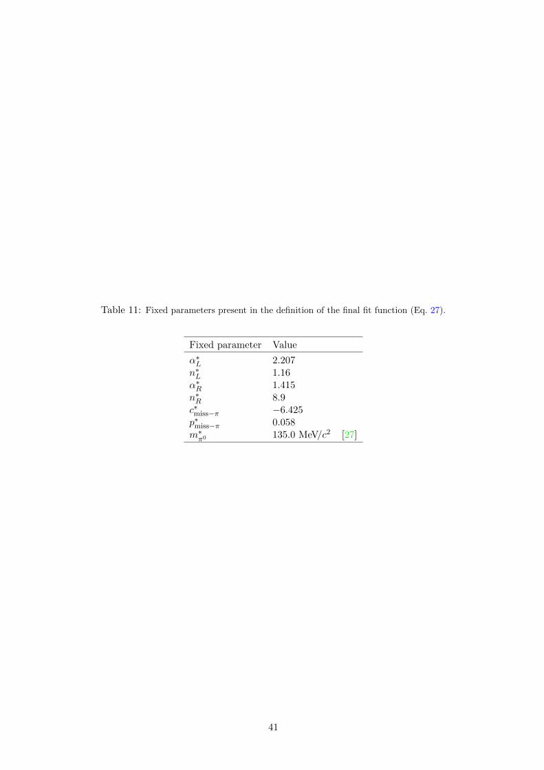
Table 11: Fixed parameters present in the definition of the final fit function (Eq. 27).

Fixed parameter Value

α∗L 2.207n∗L 1.16α∗R 1.415n∗R 8.9c∗miss−π −6.425p∗miss−π 0.058m∗π0 135.0 MeV/c2 [27]

41

6 Conclusion and outlook

This thesis has presented a selection of B± → K±π∓π±γ candidates collected by the LHCb

experiment at a centre-of-mass energy of 13 TeV. A cut-based strategy followed by the

training and application of a multivariate classifier has been described; several cuts and the

output of the classifier were optimised to maximise the significance. Approximately 3’000,

18’000 and 18’000 B± → K±π∓π±γ decays were selected in 2015, 2016 and 2017 data

samples corresponding to integrated luminosities of 0.29, 1.64 and 1.71 fb−1, respectively.

Depending on the needs of future studies, it may be useful to make a stricter cut on

the classifier output in order to increase the signal purity. Moreover, the characterisation

of background sources should be completed when more MC samples using 2016 and 2017

data-taking conditions will be available.

By adding the number of signal candidates found in the first run of the LHC [8, 9]

and the results of this study, approximately 50’000 signal decays are now available for the

measurement of the photon polarisation and the detection of a possible signal of physics

beyond the Standard Model.

As a final note, the civil-engineering work for the High-Luminosity LHC (HL-LHC)

started exactly one week before the submission of this report [41]; the upgraded machine

is designed to deliver an increased luminosity by a factor of five to seven with respect to

its current value [42]. Together with the results of other experiments such as Belle II [43],

the next decade will give us many opportunities to pursue a better understanding of how

Nature works at its most fundamental level.

Acknowledgements

I would like to express my gratitude to CERN and the LHCb collaboration without which

this project would not be possible; to my director Prof. Dr. Olivier Schneider, for his

guidance throughout my work and for having given me the opportunity to be a student-

assistant in his introduction to particle physics course; to my supervisor Dr. Preema

Pais, for her unconditional support, advices and enthusiasm; to Violaine Bellee, for all

her help and the time needed to generate the data samples; to my colleagues, for their

encouragement and comments.

42

A Appendix

A.1 Uncertainty on efficiency

Following Ref. [44], one presents here two methods to estimate the efficiency ε of a selection

where k out of n events survive a set of cuts. In this study, due to the high number of

candidates, both methods give very similar results. Unless otherwise stated, the results of

the bayesian approach is used throughout this document.

Binomial error

In the classical approach, one considers that the selection is a binomial process described

by the probability function

P (k; ε, n) =

(n

k

)εk(1− ε)n−k. (28)

The estimators of the efficiency and its uncertainty are then given by [44]ε =

k

n,

σε =

√ε(1− ε)

n=

√k(n− k)

n3.

(29)

This method cannot be correct in the general case, because it gives unphysical results

for the uncertainty in the limits k → 0 and k → n.

Bayesian approach

In a bayesian approach, one starts from the Bayes theorem and writes

P (ε; k, n) =P (k; ε, n)P (ε; n)

C, (30)

where P (ε; n) is a prior probability and C a normalisation constant. By developing this

last equation, T. Ullrich and Z. Xu obtain the estimators [44]ε =

k

n,

σε =

√(k + 1)(k + 2)

(n+ 2)(n+ 3)−(k + 1

n+ 2

)2

.

(31)

43

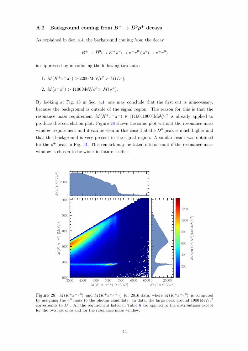
A.2 Background coming from B+ → D0ρ+ decays

As explained in Sec. 4.4, the background coming from the decay

B+ → D0(→ K+ρ−(→ π−π0))ρ+(→ π+π0)

is suppressed by introducing the following two cuts :

1. M(K+π−π0) > 2200 MeV/c2 > M(D0).

2. M(π+π0) > 1100 MeV/c2 > M(ρ+).

By looking at Fig. 13 in Sec. 4.4, one may conclude that the first cut is unnecessary,

because the background is outside of the signal region. The reason for this is that the

resonance mass requirement M(K+π−π+) ∈ [1100, 1900] MeV/c2 is already applied to

produce this correlation plot. Figure 28 shows the same plot without the resonance mass

window requirement and it can be seen in this case that the D0 peak is much higher and

that this background is very present in the signal region. A similar result was obtained

for the ρ+ peak in Fig. 14. This remark may be taken into account if the resonance mass

window is chosen to be wider in future studies.

3500 4000 4500 5000 5500 6000 6500M(K+π−π+γ) [MeV/c2]

1000

2000

3000

4000

5000

6000

M(K

+π−π

0)

[MeV

/c2]

0

20000

dN

/(30

MeV

/c2)

0 25000dN/(30 MeV/c2)

200

400

600

800

1000

1200

dN

/(30

MeV

/c2)/

(30

MeV

/c2)

Figure 28: M(K+π−π0) and M(K+π−π+γ) for 2016 data, where M(K+π−π0) is computedby assigning the π0 mass to the photon candidate. In data, the large peak around 1900 MeV/c2

corresponds to D0. All the requirement listed in Table 6 are applied to the distributions exceptfor the two last ones and for the resonance mass window.

44

A.3 2015 and 2017 data

In this appendix, several figures obtained with the 2015 and 2017 data samples are shown.

All of them correspond to figures that were presented in the main text for the 2016 data

sample. They are listed below:

• Figures 29−32 are overlay plots and correspond to Figs. 9 and 10 in the main text.

• Figures 33, 34 and 35 are correlation plots and correspond to Figs. 12, 13 and 14 in

the main text, respectively.

• Figure 36 shows correlation matrices and corresponds to Fig. 17 in the main text.

• Figure 37 shows classifiers outputs distributions and corresponds to Fig. 19 in the

main text.

45

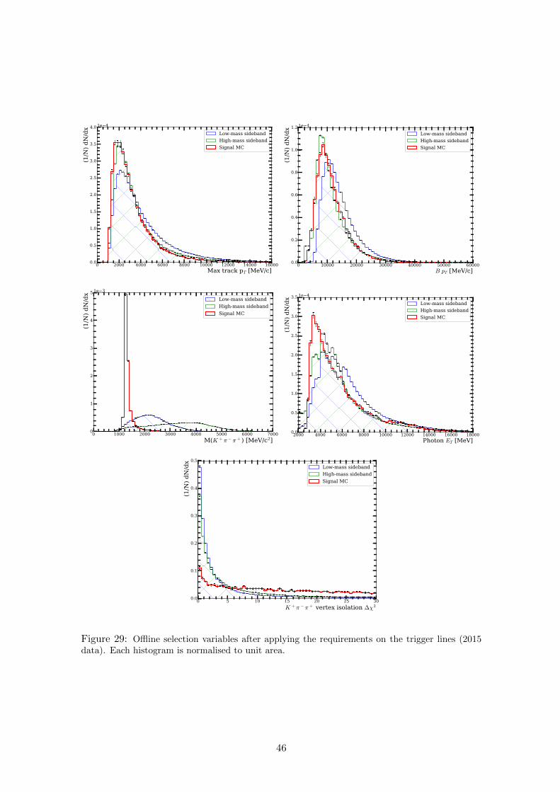
0 2000 4000 6000 8000 10000 12000 14000 16000

Max track pT [MeV/c]

0.0

0.5

1.0

1.5

2.0

2.5

3.0

3.5

4.0

(1/N

) d

N/d

x

1e 4

Low-mass sideband

High-mass sideband

Signal MC

0 10000 20000 30000 40000 50000 60000

B pT [MeV/c]

0.0

0.2

0.4

0.6

0.8

1.0

1.2

(1/N

) d

N/d

x

1e 4

Low-mass sideband

High-mass sideband

Signal MC

0 1000 2000 3000 4000 5000 6000 7000

M(K + π − π + ) [MeV/c2]

0

1

2

3

4

5

(1/N

) d

N/d

x

1e 3

Low-mass sideband

High-mass sideband

Signal MC

2000 4000 6000 8000 10000 12000 14000 16000 18000

Photon ET [MeV]

0.0

0.5

1.0

1.5

2.0

2.5

3.0

3.5

(1/N

) d

N/d

x

1e 4

Low-mass sideband

High-mass sideband

Signal MC

0 5 10 15 20 25 30

K + π − π + vertex isolation ∆χ2

0.0

0.1

0.2

0.3

0.4

0.5

(1/N

) d

N/d

x

Low-mass sideband

High-mass sideband

Signal MC

Figure 29: Offline selection variables after applying the requirements on the trigger lines (2015data). Each histogram is normalised to unit area.

46

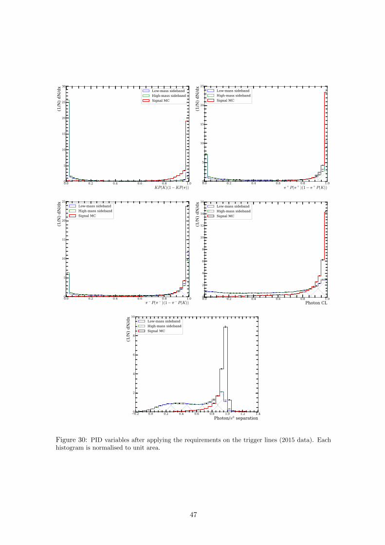
0.0 0.2 0.4 0.6 0.8 1.0

KP(K)(1−KP(π))

0

5

10

15

20

25

30

(1/N

) d

N/d

x

Low-mass sideband

High-mass sideband

Signal MC

0.0 0.2 0.4 0.6 0.8 1.0

π +P(π + )(1− π +P(K))

0

5

10

15

20

25

(1/N

) d

N/d

x

Low-mass sideband

High-mass sideband

Signal MC

0.0 0.2 0.4 0.6 0.8 1.0

π −P(π − )(1− π −P(K))

0

5

10

15

20

25

(1/N

) d

N/d

x

Low-mass sideband

High-mass sideband

Signal MC

0.0 0.2 0.4 0.6 0.8 1.0

Photon CL

0

2

4

6

8

10

12

14

16

(1/N

) d

N/d

x

Low-mass sideband

High-mass sideband

Signal MC

0.2 0.0 0.2 0.4 0.6 0.8 1.0 1.2 1.4

Photon/π0 separation

0

2

4

6

8

10

(1/N

) d

N/d

x

Low-mass sideband

High-mass sideband

Signal MC

Figure 30: PID variables after applying the requirements on the trigger lines (2015 data). Eachhistogram is normalised to unit area.

47

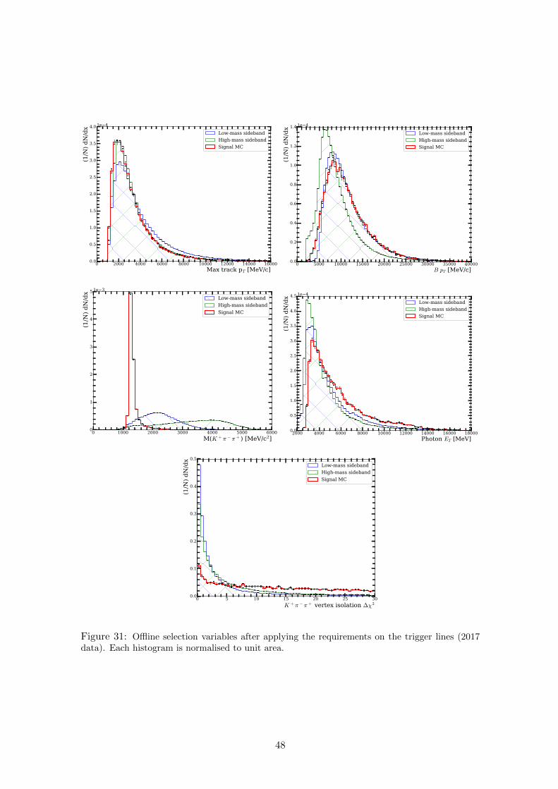
0 2000 4000 6000 8000 10000 12000 14000 16000

Max track pT [MeV/c]

0.0

0.5

1.0

1.5

2.0

2.5

3.0

3.5

4.0

(1/N

) d

N/d

x

1e 4

Low-mass sideband

High-mass sideband

Signal MC

0 5000 10000 15000 20000 25000 30000 35000 40000

B pT [MeV/c]

0.0

0.2

0.4

0.6

0.8

1.0

1.2

1.4

(1/N

) d

N/d

x

1e 4

Low-mass sideband

High-mass sideband

Signal MC

0 1000 2000 3000 4000 5000 6000

M(K + π − π + ) [MeV/c2]

0

1

2

3

4

5

(1/N

) d

N/d

x

1e 3

Low-mass sideband

High-mass sideband

Signal MC

2000 4000 6000 8000 10000 12000 14000 16000 18000

Photon ET [MeV]

0.0

0.5

1.0

1.5

2.0

2.5

3.0

3.5

4.0

4.5

(1/N

) d

N/d

x

1e 4

Low-mass sideband

High-mass sideband

Signal MC

0 5 10 15 20 25 30

K + π − π + vertex isolation ∆χ2

0.0

0.1

0.2

0.3

0.4

0.5

(1/N

) d

N/d

x

Low-mass sideband

High-mass sideband

Signal MC

Figure 31: Offline selection variables after applying the requirements on the trigger lines (2017data). Each histogram is normalised to unit area.

48

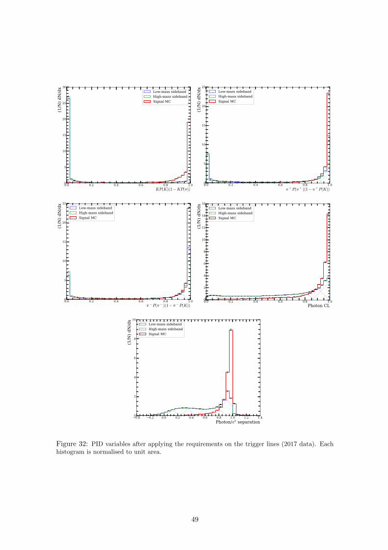
0.0 0.2 0.4 0.6 0.8 1.0

KP(K)(1−KP(π))

0

5

10

15

20

25

30

(1/N

) d

N/d

x

Low-mass sideband

High-mass sideband

Signal MC

0.0 0.2 0.4 0.6 0.8 1.0

π +P(π + )(1− π +P(K))

0

5

10

15

20

25

(1/N

) d

N/d

x

Low-mass sideband

High-mass sideband

Signal MC

0.0 0.2 0.4 0.6 0.8 1.0

π −P(π − )(1− π −P(K))

0

5

10

15

20

25

(1/N

) d

N/d

x

Low-mass sideband

High-mass sideband

Signal MC

0.0 0.2 0.4 0.6 0.8 1.0

Photon CL

0

2

4

6

8

10

12

14

16

(1/N

) d

N/d

x

Low-mass sideband

High-mass sideband

Signal MC

0.4 0.2 0.0 0.2 0.4 0.6 0.8 1.0 1.2 1.4

Photon/π0 separation

0

2

4

6

8

10

(1/N

) d

N/d

x

Low-mass sideband

High-mass sideband

Signal MC

Figure 32: PID variables after applying the requirements on the trigger lines (2017 data). Eachhistogram is normalised to unit area.

49

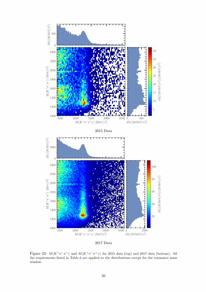
4500 5000 5500 6000 6500M(K+π−π+γ) [MeV/c2]

1000

1200

1400

1600

1800

2000

2200

2400

M(K

+π−π

+)

[MeV

/c2]

0

500

dN

/(30

MeV

/c2)

0 500dN/(30 MeV/c2)

5

10

15

20

25

30

35

40

dN

/(30

MeV

/c2)/

(30

MeV

/c2)

2015 Data

4500 5000 5500 6000 6500M(K+π−π+γ) [MeV/c2]

1000

1200

1400

1600

1800

2000

2200

2400

M(K

+π−π

+)

[MeV

/c2]

0

2000

dN

/(20

MeV

/c2)

0 2500dN/(20 MeV/c2)

20

40

60

80

100

dN

/(20

MeV

/c2)/

(20

MeV

/c2)

2017 Data

Figure 33: M(K+π−π+) and M(K+π−π+γ) for 2015 data (top) and 2017 data (bottom). Allthe requirements listed in Table 6 are applied to the distributions except for the resonance masswindow.

50

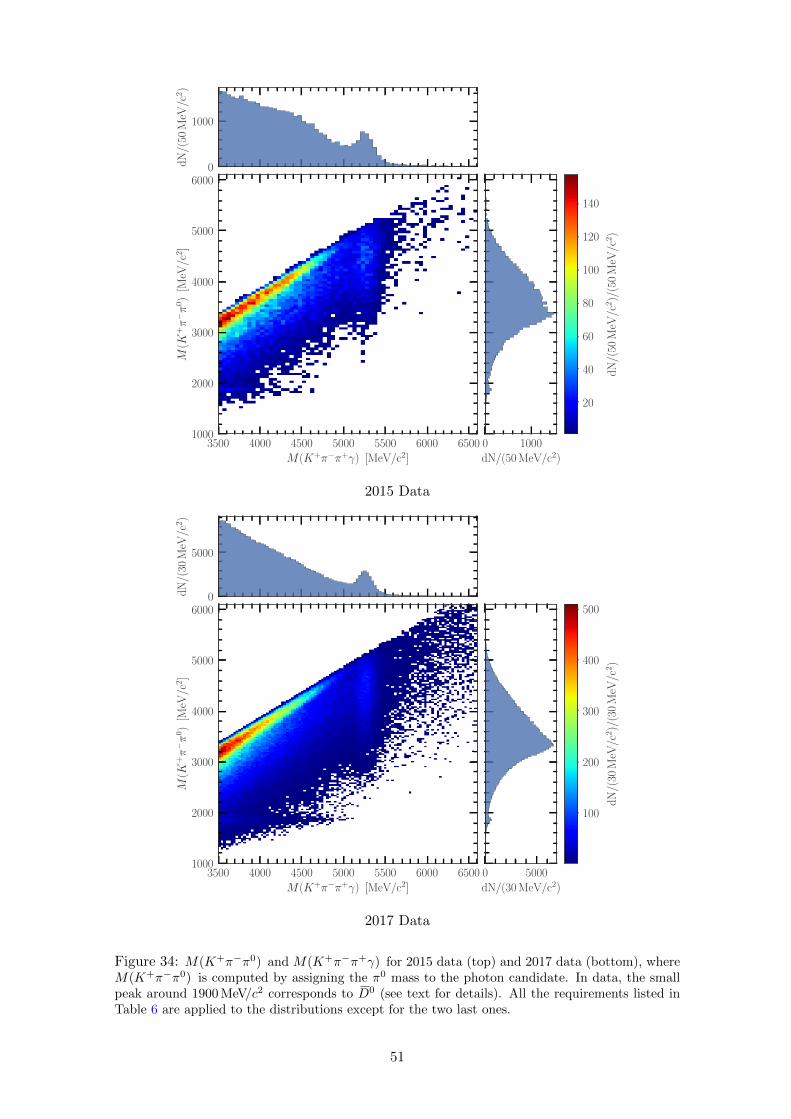
3500 4000 4500 5000 5500 6000 6500M(K+π−π+γ) [MeV/c2]

1000

2000

3000

4000

5000

6000M

(K+π−π

0)

[MeV

/c2]

0

1000

dN

/(50

MeV

/c2)

0 1000dN/(50 MeV/c2)

20

40

60

80

100

120

140

dN

/(50

MeV

/c2)/

(50

MeV

/c2)

2015 Data

3500 4000 4500 5000 5500 6000 6500M(K+π−π+γ) [MeV/c2]

1000

2000

3000

4000

5000

6000

M(K

+π−π

0)

[MeV

/c2]

0

5000

dN

/(30

MeV

/c2)

0 5000dN/(30 MeV/c2)

100

200

300

400

500d

N/(

30M

eV/c

2)/

(30

MeV

/c2)

2017 Data

Figure 34: M(K+π−π0) and M(K+π−π+γ) for 2015 data (top) and 2017 data (bottom), whereM(K+π−π0) is computed by assigning the π0 mass to the photon candidate. In data, the smallpeak around 1900 MeV/c2 corresponds to D0 (see text for details). All the requirements listed inTable 6 are applied to the distributions except for the two last ones.

51

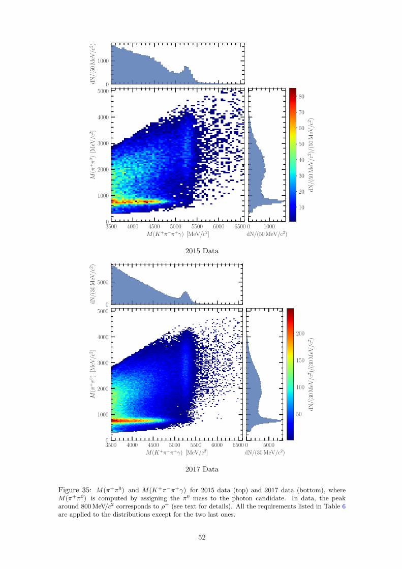
3500 4000 4500 5000 5500 6000 6500M(K+π−π+γ) [MeV/c2]

0

1000

2000

3000

4000

5000M

(π+π

0)

[MeV

/c2]

0

1000

dN

/(50

MeV

/c2)

0 1000dN/(50 MeV/c2)

10

20

30

40

50

60

70

80

dN

/(50

MeV

/c2)/

(50

MeV

/c2)

2015 Data

3500 4000 4500 5000 5500 6000 6500M(K+π−π+γ) [MeV/c2]

0

1000

2000

3000

4000

5000

M(π

+π

0)

[MeV

/c2]

0

5000

dN

/(30

MeV

/c2)

0 5000dN/(30 MeV/c2)

50

100

150

200

dN

/(30

MeV

/c2)/

(30

MeV

/c2)

2017 Data

Figure 35: M(π+π0) and M(K+π−π+γ) for 2015 data (top) and 2017 data (bottom), whereM(π+π0) is computed by assigning the π0 mass to the photon candidate. In data, the peakaround 800 MeV/c2 corresponds to ρ+ (see text for details). All the requirements listed in Table 6are applied to the distributions except for the two last ones.

52

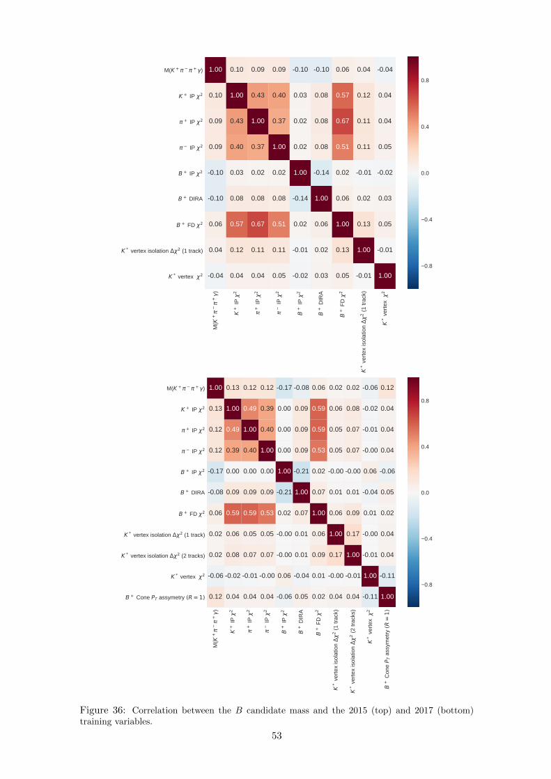
M(K

++

)

K+

 IP 

2

+ IP

 2

 IP 

2

B+

 IP 

2

B+

 DIR

A

B+

 FD

 2

K*  

vert

ex is

olat

ion 

2  (1

 trac

k)

K*  

vert

ex  

2

K *  vertex   2

K *  vertex isolation  2 (1 track)

B +  FD  2

B +  DIRA

B +  IP  2

 IP  2

+  IP  2

K +  IP  2

M(K + + )

­0.04 0.04 0.04 0.05 ­0.02 0.03 0.05 ­0.01 1.00

0.04 0.12 0.11 0.11 ­0.01 0.02 0.13 1.00 ­0.01

0.06 0.57 0.67 0.51 0.02 0.06 1.00 0.13 0.05

­0.10 0.08 0.08 0.08 ­0.14 1.00 0.06 0.02 0.03

­0.10 0.03 0.02 0.02 1.00 ­0.14 0.02 ­0.01 ­0.02

0.09 0.40 0.37 1.00 0.02 0.08 0.51 0.11 0.05

0.09 0.43 1.00 0.37 0.02 0.08 0.67 0.11 0.04

0.10 1.00 0.43 0.40 0.03 0.08 0.57 0.12 0.04

1.00 0.10 0.09 0.09 ­0.10 ­0.10 0.06 0.04 ­0.04

0.8

0.4

0.0

0.4

0.8

M(K

++

)

K+

 IP 

2

+ IP

 2

 IP 

2

B+

 IP 

2

B+

 DIR

A

B+

 FD

 2

K*  

vert

ex is

olat

ion 

2  (1

 trac

k)

K*  

vert

ex is

olat

ion 

2  (2

 trac

ks)

K*  

vert

ex  

2

B+

 Con

e P T

 ass

ymet

ry (R

=1)

B +  Cone PT assymetry (R = 1)

K *  vertex   2

K *  vertex isolation  2 (2 tracks)

K *  vertex isolation  2 (1 track)

B +  FD  2

B +  DIRA

B +  IP  2

 IP  2

+  IP  2

K +  IP  2

M(K + + )

0.12 0.04 0.04 0.04 ­0.06 0.05 0.02 0.04 0.04 ­0.11 1.00

­0.06 ­0.02 ­0.01 ­0.00 0.06 ­0.04 0.01 ­0.00 ­0.01 1.00 ­0.11

0.02 0.08 0.07 0.07 ­0.00 0.01 0.09 0.17 1.00 ­0.01 0.04

0.02 0.06 0.05 0.05 ­0.00 0.01 0.06 1.00 0.17 ­0.00 0.04

0.06 0.59 0.59 0.53 0.02 0.07 1.00 0.06 0.09 0.01 0.02

­0.08 0.09 0.09 0.09 ­0.21 1.00 0.07 0.01 0.01 ­0.04 0.05

­0.17 0.00 0.00 0.00 1.00 ­0.21 0.02 ­0.00 ­0.00 0.06 ­0.06

0.12 0.39 0.40 1.00 0.00 0.09 0.53 0.05 0.07 ­0.00 0.04

0.12 0.49 1.00 0.40 0.00 0.09 0.59 0.05 0.07 ­0.01 0.04

0.13 1.00 0.49 0.39 0.00 0.09 0.59 0.06 0.08 ­0.02 0.04

1.00 0.13 0.12 0.12 ­0.17 ­0.08 0.06 0.02 0.02 ­0.06 0.12

0.8

0.4

0.0

0.4

0.8

Figure 36: Correlation between the B candidate mass and the 2015 (top) and 2017 (bottom)training variables.

53

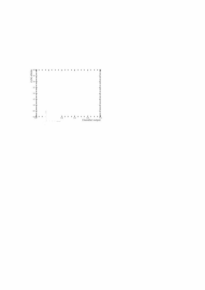
0.0 0.2 0.4 0.6 0.8 1.0Classifier output

0.0

0.5

1.0

1.5

2.0

2.5

3.0

3.5

4.0

(1/N

) dN

/dx

Kolmogorov-Smirnov test: signal (background) p-value = 0.916 (0.287)Signal (test)Background (test)

Signal (training)Background (training)

0.0 0.2 0.4 0.6 0.8 1.0Classifier output

0.0

0.5

1.0

1.5

2.0

2.5

3.0

3.5

(1/N

) dN

/dx

Kolmogorov-Smirnov test: signal (background) p-value = 0.288 (0.890)Signal (test)Background (test)

Signal (training)Background (training)

2015 Data

0.0 0.2 0.4 0.6 0.8 1.0Classifier output

0.0

0.5

1.0

1.5

2.0

2.5

3.0

3.5

4.0

(1/N

) dN

/dx

Kolmogorov-Smirnov test: signal (background) p-value = 0.316 (0.303)Signal (test)Background (test)

Signal (training)Background (training)

0.0 0.2 0.4 0.6 0.8 1.0Classifier output

0.0

0.5

1.0

1.5

2.0

2.5

3.0

3.5

4.0

(1/N

) dN

/dx

Kolmogorov-Smirnov test: signal (background) p-value = 0.279 (0.383)Signal (test)Background (test)

Signal (training)Background (training)

2017 Data

Figure 37: Distribution of two classifiers outputs and comparison between the results obtainedwith the training and test sets. The first classifier (left) is trained on A0B0 and tested on A0B1;the second classifier (right) is trained on A1B0 and tested on A1B1. Comparison between 2015data (top) and 2017 data (bottom).

54

References

[1] F. Zwicky, On the masses of nebulae and of clusters of nebulae, Astrophys. J. 86

(1937) 217.

[2] D. Clowe, M. Bradac, A. H. Gonzalez, M. Markevitch, S. W. Randall, C. Jones

et al., A direct empirical proof of the existence of dark matter, Astrophys. J. 648

(2006) L109 [astro-ph/0608407].

[3] Planck collaboration, P. A. R. Ade et al., Planck 2015 results. XIII. Cosmological

parameters, Astron. Astrophys. 594 (2016) A13 [1502.01589].

[4] M. Gronau, Y. Grossman, D. Pirjol and A. Ryd, Measuring the photon polarization

in B → Kππγ, Phys. Rev. Lett. 88 (2002) 051802 [hep-ph/0107254].

[5] M. Gronau and D. Pirjol, Photon polarization in radiative B decays, Phys. Rev.

D66 (2002) 054008 [hep-ph/0205065].

[6] D. Becirevic, E. Kou, A. Le Yaouanc and A. Tayduganov, Future prospects for the

determination of the Wilson coefficient C ′7γ , JHEP 08 (2012) 090 [1206.1502].

[7] I. Leboucq, Observation of the decay B+ → K+π−π+γ at LHCb, Master thesis,

EPFL, 2012.

[8] G. Veneziano, Towards the measurement of photon polarisation in the decay

B+ → K+π−π+γ, Ph.D. thesis, EPFL, 2016.

[9] A. Puig Navarro, First measurements of radiative B decays in LHCb, Ph.D. thesis,

Barcelona U., 2012.

[10] LHCb collaboration, R. Aaij et al., Observation of photon polarization in the b→ sγ

transition, Phys. Rev. Lett. 112 (2014) 161801 [1402.6852].

[11] C. Mordasini, Study of the B+ → K+π−π+γ selection at LHCb, Master thesis,

EPFL, 2017.

[12] S. L. Glashow, Partial symmetries of weak interactions, Nucl. Phys. 22 (1961) 579.

[13] S. Weinberg, A model of leptons, Phys. Rev. Lett. 19 (1967) 1264.

[14] D. Galbraith and C. Burgard, Standard model, standard infographic, 2012.

[15] M. Kobayashi and T. Maskawa, CP violation in the renormalizable theory of weak

interaction, Prog. Theor. Phys. 49 (1973) 652.

[16] J. Ellis, TikZ-Feynman: Feynman diagrams with TikZ, Comput. Phys. Commun.

210 (2017) 103 [1601.05437].

[17] LHCb collaboration, A. A. Alves, Jr. et al., The LHCb detector at the LHC, JINST

3 (2008) S08005.

55

[18] R. Aaij et al., Performance of the LHCb Vertex Locator, JINST 9 (2014) P09007

[1405.7808].

[19] A. Coccaro, Track reconstruction and b-jet identification for the ATLAS trigger

system, J. Phys. Conf. Ser. 368 (2012) 012034 [1112.0180].

[20] LHCb Outer Tracker group, P. d’Argent et al., Improved performance of the LHCb

Outer Tracker in LHC Run 2, JINST 12 (2017) P11016 [1708.00819].

[21] LHCb collaboration, E. Michielin, The LHCb trigger in Run II, PoS ICHEP2016

(2016) 996.

[22] LHCb collaboration, B. Sciascia, LHCb Run 2 trigger performance, PoS

BEAUTY2016 (2016) 029.

[23] T. Sjostrand, S. Ask, J. R. Christiansen, R. Corke, N. Desai, P. Ilten et al., An

introduction to PYTHIA 8.2, Comput. Phys. Commun. 191 (2015) 159 [1410.3012].

[24] GEANT4 collaboration, S. Agostinelli et al., GEANT4: A simulation toolkit, Nucl.

Instrum. Meth. A506 (2003) 250.

[25] LHCb Starterkit team, A. Puig, The LHCb Starterkit, J. Phys. Conf. Ser. 898

(2017) 082054.

[26] LHCb collaboration, R. Aaij et al., Measurement of the B± production cross-section

in pp collisions at√s = 7 and 13 TeV, JHEP 12 (2017) 026 [1710.04921].

[27] Particle Data Group, C. Patrignani et al., Review of Particle Physics, Chin. Phys.

C40 (2016) 100001.

[28] R. Aaij et al., Selection and processing of calibration samples to measure the particle

identification performance of the LHCb experiment in Run 2, 1803.00824.

[29] T. Hastie, R. Tibshirani and J. Friedman, The elements of statistical learning,

Springer Series in Statistics. Springer New York Inc., New York, NY, USA, 2001.

[30] T. Chen and C. Guestrin, XGBoost: A scalable tree boosting system, in Proceedings

of the 22nd ACM SIGKDD International Conference on Knowledge Discovery and

Data Mining, KDD ’16, (New York, NY, USA), pp. 785–794, ACM, 2016,

1603.02754.

[31] L. Breiman, Random forests, Machine Learning 45 (2001) 5.

[32] F. Pedregosa et al., Scikit-learn: Machine learning in Python, J. Machine Learning

Res. 12 (2011) 2825 [1201.0490].

[33] A. Muller and S. Guido, Introduction to machine learning with Python: A guide for

data scientists. O’Reilly, 2016.

56

[34] CDF collaboration, A. Abulencia et al., Search for Bs → µ+µ− and Bd → µ+µ−

decays in pp collisions with CDF II, Phys. Rev. Lett. 95 (2005) 221805

[hep-ex/0508036].

[35] M. Chrzaszcz, Search for charged lepton flavour violation at LHCb experiment,

Ph.D. thesis, Cracow, INP, 2014-11-07.

[36] A. Hoecker, P. Speckmayer, J. Stelzer, J. Therhaag, E. von Toerne and H. Voss,

TMVA: Toolkit for Multivariate Data Analysis, PoS ACAT (2007) 040

[physics/0703039].

[37] R. Brun and F. Rademakers, ROOT: An object oriented data analysis framework,

Nucl. Instrum. Meth. A389 (1997) 81.

[38] W. Verkerke and D. P. Kirkby, The RooFit toolkit for data modeling, eConf

C0303241 (2003) MOLT007 [physics/0306116].

[39] T. Skwarnicki, A study of the radiative CASCADE transitions between the

Upsilon-Prime and Upsilon resonances, Ph.D. thesis, Cracow, INP, 1986.

[40] ARGUS collaboration, H. Albrecht et al., Search for hadronic b→ u decays, Phys.

Lett. B241 (1990) 278.

[41] C. Pralavorio, Major work starts to boost the luminosity of the LHC, www. cern. ch

(2018) Accessed: 15.06.2018.

[42] G. Apollinari, O. Brning, T. Nakamoto and L. Rossi, High Luminosity Large

Hadron Collider HL-LHC, CERN Yellow Report (2015) 1 [1705.08830].

[43] J. Bennett, The Belle II experiment: status and physics prospects, Int. J. Mod.

Phys. Conf. Ser. 46 (2018) 1860082.

[44] T. Ullrich and Z. Xu, Treatment of errors in efficiency calculations, 2007,

physics/0701199v1.

57