Optimal rate of convergence in periodic homogenization of ...
33
Optimal rate of convergence in periodic homogenization of Hamilton-Jacobi equations Hung V. Tran Department of Mathematics – UW Madison joint works with W. Jing, H. Mitake, and Y. Yu CNA Seminar, CMU, January 2020 Hung V. Tran (UW Madison) Optimal rate of convergence 1 / 22
Transcript of Optimal rate of convergence in periodic homogenization of ...
Optimal rate of convergence in periodic homogenizationof Hamilton-Jacobi equations
Hung V. Tran
Department of Mathematics – UW Madison
joint works with W. Jing, H. Mitake, and Y. Yu
CNA Seminar, CMU, January 2020
Hung V. Tran (UW Madison) Optimal rate of convergence 1 / 22
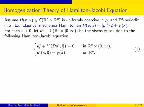
Homogenization Theory of Hamilton-Jacobi Equation
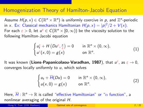
Assume H(p, x) ∈ C (Rn × Rn) is uniformly coercive in p, and Zn-periodicin x . Ex: Classical mechanics Hamiltonian H(p, x) = |p|2/2 + V (x).For each ε > 0, let uε ∈ C (Rn × [0,∞)) be the viscosity solution to thefollowing Hamilton-Jacobi equation{
uεt + H(Duε, xε
)= 0 in Rn × (0,∞),
uε(x , 0) = g(x) on Rn.(1)
It was known (Lions-Papanicolaou-Varadhan, 1987), that uε, as ε→ 0,converges locally uniformly to u, which solves{
ut + H(Du) = 0 in Rn × (0,∞),
u(x , 0) = g(x) on Rn.(2)
Here, H : Rn → R is called “effective Hamiltonian” or “α function”, anonlinear averaging of the original H.
Hung V. Tran (UW Madison) Optimal rate of convergence 2 / 22
Homogenization Theory of Hamilton-Jacobi Equation
Assume H(p, x) ∈ C (Rn × Rn) is uniformly coercive in p, and Zn-periodicin x . Ex: Classical mechanics Hamiltonian H(p, x) = |p|2/2 + V (x).For each ε > 0, let uε ∈ C (Rn × [0,∞)) be the viscosity solution to thefollowing Hamilton-Jacobi equation{
uεt + H(Duε, xε
)= 0 in Rn × (0,∞),
uε(x , 0) = g(x) on Rn.(1)
It was known (Lions-Papanicolaou-Varadhan, 1987), that uε, as ε→ 0,converges locally uniformly to u, which solves{
ut + H(Du) = 0 in Rn × (0,∞),
u(x , 0) = g(x) on Rn.(2)
Here, H : Rn → R is called “effective Hamiltonian” or “α function”, anonlinear averaging of the original H.
Hung V. Tran (UW Madison) Optimal rate of convergence 2 / 22
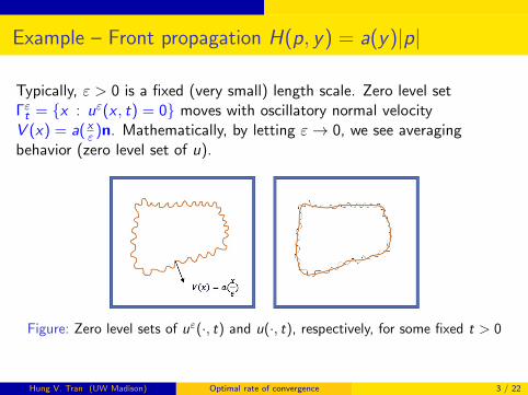
Example – Front propagation H(p, y) = a(y)|p|
Typically, ε > 0 is a fixed (very small) length scale. Zero level setΓεt = {x : uε(x , t) = 0} moves with oscillatory normal velocityV (x) = a( xε )n. Mathematically, by letting ε→ 0, we see averagingbehavior (zero level set of u).
Figure: Zero level sets of uε(·, t) and u(·, t), respectively, for some fixed t > 0
Hung V. Tran (UW Madison) Optimal rate of convergence 3 / 22
Cell problems and effective Hamiltonian
For any p ∈ Rn, there exists a UNIQUE number H(p) ∈ R such that
H(p + Dv , y) = H(p) in Tn.
has a periodic viscosity solution v (often named corrector). Writev = v(y , p) to demonstrate clear dependence.
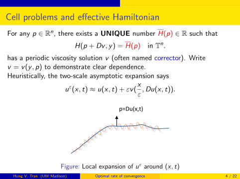
Heuristically, the two-scale asymptotic expansion says
uε(x , t) ≈ u(x , t) + εv(x
ε,Du(x , t)).
p=Du(x,t)
Figure: Local expansion of uε around (x , t)
Hung V. Tran (UW Madison) Optimal rate of convergence 4 / 22
Cell problems and effective Hamiltonian
For any p ∈ Rn, there exists a UNIQUE number H(p) ∈ R such that
H(p + Dv , y) = H(p) in Tn.
has a periodic viscosity solution v (often named corrector). Writev = v(y , p) to demonstrate clear dependence.Heuristically, the two-scale asymptotic expansion says
uε(x , t) ≈ u(x , t) + εv(x
ε,Du(x , t)).
p=Du(x,t)
Figure: Local expansion of uε around (x , t)
Hung V. Tran (UW Madison) Optimal rate of convergence 4 / 22
Main question of interest
Heuristically, the two-scale asymptotic expansion says:
uε(x , t) ≈ u(x , t) + εv(x
ε,Du(x , t)).
Note: The corrector v(y , p) for p = Du(x , t) basically captures (corrects)the oscillation of Duε around (x , t). Here, y = x
ε .
A natural and fundamental question
How fast does uε converge to u as ε→ 0+?
According to the above formal expansion, it seems that
|uε − u| = O(ε).
However, there is NO way to justify this expansion rigorously!
Hung V. Tran (UW Madison) Optimal rate of convergence 5 / 22
Previous Results
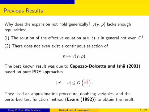
Why does the expansion not hold generically? v(y , p) lacks enoughregularities:
(I) The solution of the effective equation u(x , t) is in general not even C 1;
(2) There does not even exist a continuous selection of
p 7→ v(y , p).
The best known result was due to Capuzzo-Dolcetta and Ishii (2001)based on pure PDE approaches
|uε − u| ≤ O(ε
13
).
They used an approximation procedure, doubling variables, and theperturbed test function method (Evans (1992)) to obtain the result.
Hung V. Tran (UW Madison) Optimal rate of convergence 6 / 22
Previous Results
Why does the expansion not hold generically? v(y , p) lacks enoughregularities:
(I) The solution of the effective equation u(x , t) is in general not even C 1;
(2) There does not even exist a continuous selection of
p 7→ v(y , p).
The best known result was due to Capuzzo-Dolcetta and Ishii (2001)based on pure PDE approaches
|uε − u| ≤ O(ε
13
).
They used an approximation procedure, doubling variables, and theperturbed test function method (Evans (1992)) to obtain the result.
Hung V. Tran (UW Madison) Optimal rate of convergence 6 / 22
Main Result 1: General Convex Case (p → H(p, x))
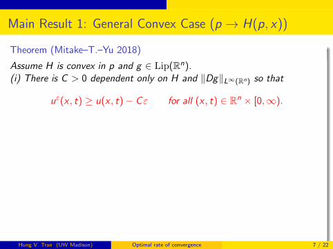
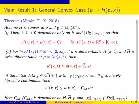
Theorem (Mitake–T.–Yu 2018)
Assume H is convex in p and g ∈ Lip(Rn).(i) There is C > 0 dependent only on H and ‖Dg‖L∞(Rn) so that
uε(x , t) ≥ u(x , t)− Cε for all (x , t) ∈ Rn × [0,∞).
(ii) For fixed (x , t) ∈ Rn × (0,∞), if u is differentiable at (x , t), and H istwice differentiable at p = Du(x , t), then
uε(x , t) ≤ u(x , t) + C̃x ,tε.
if the initial data g ∈ C 2(Rn) with ‖g‖C2(Rn) <∞. If g is merelyLipschitz continuous, then
uε(x , t) ≤ u(x , t) + Cx ,t√ε.
Here C̃x ,t (Cx ,t) is dependent on H,H, p and ‖g‖C2(Rn) (‖Dg‖L∞(Rn)).
Hung V. Tran (UW Madison) Optimal rate of convergence 7 / 22
Main Result 1: General Convex Case (p → H(p, x))
Theorem (Mitake–T.–Yu 2018)
Assume H is convex in p and g ∈ Lip(Rn).(i) There is C > 0 dependent only on H and ‖Dg‖L∞(Rn) so that
uε(x , t) ≥ u(x , t)− Cε for all (x , t) ∈ Rn × [0,∞).
(ii) For fixed (x , t) ∈ Rn × (0,∞), if u is differentiable at (x , t), and H istwice differentiable at p = Du(x , t), then
uε(x , t) ≤ u(x , t) + C̃x ,tε.
if the initial data g ∈ C 2(Rn) with ‖g‖C2(Rn) <∞. If g is merelyLipschitz continuous, then
uε(x , t) ≤ u(x , t) + Cx ,t√ε.
Here C̃x ,t (Cx ,t) is dependent on H,H, p and ‖g‖C2(Rn) (‖Dg‖L∞(Rn)).Hung V. Tran (UW Madison) Optimal rate of convergence 7 / 22
Main result 2: Two dimensions
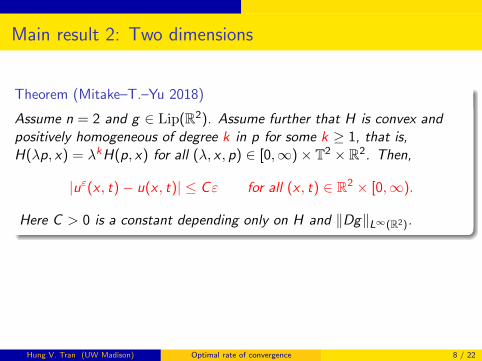
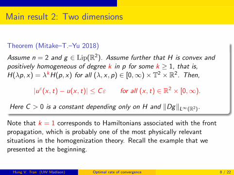
Theorem (Mitake–T.–Yu 2018)
Assume n = 2 and g ∈ Lip(R2). Assume further that H is convex andpositively homogeneous of degree k in p for some k ≥ 1, that is,H(λp, x) = λkH(p, x) for all (λ, x , p) ∈ [0,∞)× T2 × R2. Then,
|uε(x , t)− u(x , t)| ≤ Cε for all (x , t) ∈ R2 × [0,∞).
Here C > 0 is a constant depending only on H and ‖Dg‖L∞(R2).
Note that k = 1 corresponds to Hamiltonians associated with the frontpropagation, which is probably one of the most physically relevantsituations in the homogenization theory. Recall the example that wepresented at the beginning.
Hung V. Tran (UW Madison) Optimal rate of convergence 8 / 22
Main result 2: Two dimensions
Theorem (Mitake–T.–Yu 2018)
Assume n = 2 and g ∈ Lip(R2). Assume further that H is convex andpositively homogeneous of degree k in p for some k ≥ 1, that is,H(λp, x) = λkH(p, x) for all (λ, x , p) ∈ [0,∞)× T2 × R2. Then,
|uε(x , t)− u(x , t)| ≤ Cε for all (x , t) ∈ R2 × [0,∞).
Here C > 0 is a constant depending only on H and ‖Dg‖L∞(R2).
Note that k = 1 corresponds to Hamiltonians associated with the frontpropagation, which is probably one of the most physically relevantsituations in the homogenization theory. Recall the example that wepresented at the beginning.
Hung V. Tran (UW Madison) Optimal rate of convergence 8 / 22
Main result 3: One dimension
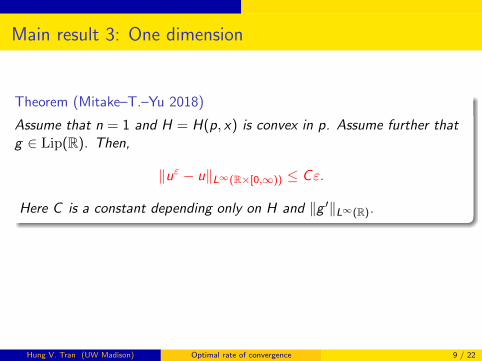
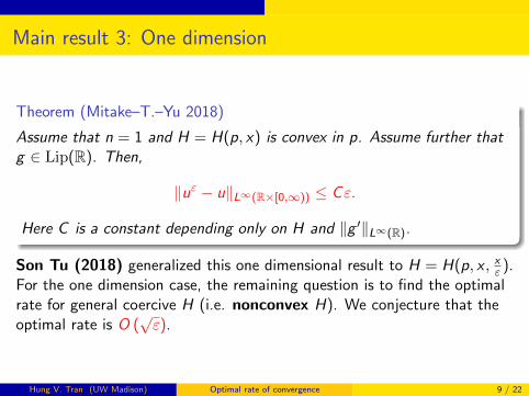
Theorem (Mitake–T.–Yu 2018)
Assume that n = 1 and H = H(p, x) is convex in p. Assume further thatg ∈ Lip(R). Then,
‖uε − u‖L∞(R×[0,∞)) ≤ Cε.
Here C is a constant depending only on H and ‖g ′‖L∞(R).
Son Tu (2018) generalized this one dimensional result to H = H(p, x , xε ).For the one dimension case, the remaining question is to find the optimalrate for general coercive H (i.e. nonconvex H). We conjecture that theoptimal rate is O (
√ε).
Hung V. Tran (UW Madison) Optimal rate of convergence 9 / 22
Main result 3: One dimension
Theorem (Mitake–T.–Yu 2018)
Assume that n = 1 and H = H(p, x) is convex in p. Assume further thatg ∈ Lip(R). Then,
‖uε − u‖L∞(R×[0,∞)) ≤ Cε.
Here C is a constant depending only on H and ‖g ′‖L∞(R).
Son Tu (2018) generalized this one dimensional result to H = H(p, x , xε ).For the one dimension case, the remaining question is to find the optimalrate for general coercive H (i.e. nonconvex H). We conjecture that theoptimal rate is O (
√ε).
Hung V. Tran (UW Madison) Optimal rate of convergence 9 / 22
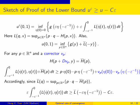
Sketch of Proof of the Lower Bound uε ≥ u − Cε
uε(0, 1) = infη(0)=0
{g(εη(−ε−1
))+ ε
∫ 0
−ε−1
L(η̇(t), η(t)) dt
}Here L(q, x) = supp∈Rn{p · q − H(p, x)}. Also,
u(0, 1) = infy∈Rn
{g(y) + L(−y)
}.
For any p ∈ Rn and a corrector vp:
H(p + Dvp, y) = H(p),∫ 0
−ε−1
L(η̇(t), η(t))+H(p) dt ≥ p·η(0)−p·η(−ε−1
)+vp(η(0))−vp
(η(−ε−1
)).
Accordingly, since L(q) = supp∈Rn{p · q − H(p)},
ε
∫ 0
−ε−1
(L(η̇(t), η(t)) dt ≥ L(−εη
(−ε−1
))− Cε.
Hung V. Tran (UW Madison) Optimal rate of convergence 10 / 22
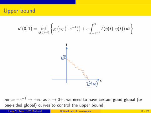
Upper bound
uε(0, 1) = infη(0)=0
{g(εη(−ε−1
))+ ε
∫ 0
−ε−1
L(η̇(t), η(t)) dt
}
x
t
Since −ε−1 → −∞ as ε→ 0+, we need to have certain good global (orone-sided global) curves to control the upper bound.
Hung V. Tran (UW Madison) Optimal rate of convergence 11 / 22
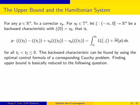
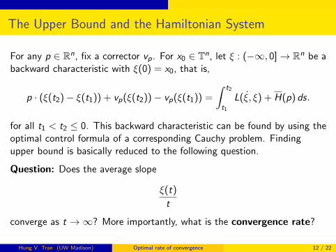
The Upper Bound and the Hamiltonian System
For any p ∈ Rn, fix a corrector vp. For x0 ∈ Tn, let ξ : (−∞, 0]→ Rn be abackward characteristic with ξ(0) = x0, that is,
p · (ξ(t2)− ξ(t1)) + vp(ξ(t2))− vp(ξ(t1)) =
∫ t2
t1
L(ξ̇, ξ) + H(p) ds.
for all t1 < t2 ≤ 0. This backward characteristic can be found by using theoptimal control formula of a corresponding Cauchy problem. Findingupper bound is basically reduced to the following question.
Question: Does the average slope
ξ(t)
t
converge as t →∞? More importantly, what is the convergence rate?
Hung V. Tran (UW Madison) Optimal rate of convergence 12 / 22
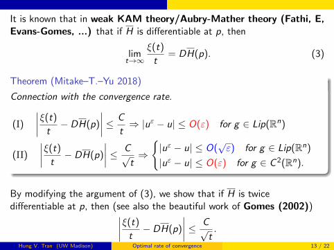
It is known that in weak KAM theory/Aubry-Mather theory (Fathi, E,Evans-Gomes, ...) that if H is differentiable at p, then
limt→∞
ξ(t)
t= DH(p). (3)
Theorem (Mitake–T.–Yu 2018)
Connection with the convergence rate.
(I)
∣∣∣∣ξ(t)
t− DH(p)
∣∣∣∣ ≤ C
t⇒ |uε − u| ≤ O(ε) for g ∈ Lip(Rn)
(II)
∣∣∣∣ξ(t)
t− DH(p)
∣∣∣∣ ≤ C√t⇒
{|uε − u| ≤ O(
√ε) for g ∈ Lip(Rn)
|uε − u| ≤ O(ε) for g ∈ C 2(Rn).
By modifying the argument of (3), we show that if H is twicedifferentiable at p, then (see also the beautiful work of Gomes (2002))∣∣∣∣ξ(t)
t− DH(p)
∣∣∣∣ ≤ C√t.
Hung V. Tran (UW Madison) Optimal rate of convergence 13 / 22
Two dimensions and the Aubry-Mather Theory
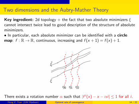
Key ingredient: 2d topology + the fact that two absolute minimizers ξcannot intersect twice lead to good description of the structure of absoluteminimizers.
• In particular, each absolute minimizer can be identified with a circlemap: f : R→ R, continuous, increasing and f (x + 1) = f (x) + 1.
ξ̃
ξ
η0 η1 η2
There exists a rotation number α such that |f i (x)− x − αi | ≤ 1 for all i .
Hung V. Tran (UW Madison) Optimal rate of convergence 14 / 22
Two dimensions and the Aubry-Mather Theory
Key ingredient: 2d topology + the fact that two absolute minimizers ξcannot intersect twice lead to good description of the structure of absoluteminimizers.• In particular, each absolute minimizer can be identified with a circlemap: f : R→ R, continuous, increasing and f (x + 1) = f (x) + 1.
ξ̃
ξ
η0 η1 η2
There exists a rotation number α such that |f i (x)− x − αi | ≤ 1 for all i .Hung V. Tran (UW Madison) Optimal rate of convergence 14 / 22
Connection with the Convergence Rate
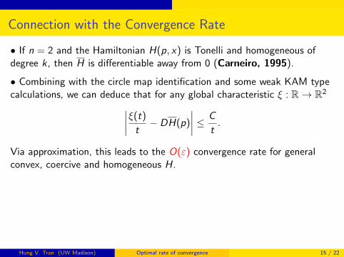
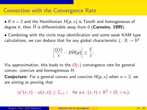
• If n = 2 and the Hamiltonian H(p, x) is Tonelli and homogeneous ofdegree k , then H is differentiable away from 0 (Carneiro, 1995).
• Combining with the circle map identification and some weak KAM typecalculations, we can deduce that for any global characteristic ξ : R→ R2∣∣∣∣ξ(t)
t− DH(p)
∣∣∣∣ ≤ C
t.
Via approximation, this leads to the O(ε) convergence rate for generalconvex, coercive and homogeneous H.
Conjecture: For a general convex and coercive H(p, x) when n = 2, weare aiming at proving that
|uε(x , t)− u(x , t)| ≤ Cx ,t ε for a.e. (x , t) ∈ R2 × (0,+∞).
Hung V. Tran (UW Madison) Optimal rate of convergence 15 / 22
Connection with the Convergence Rate
• If n = 2 and the Hamiltonian H(p, x) is Tonelli and homogeneous ofdegree k , then H is differentiable away from 0 (Carneiro, 1995).
• Combining with the circle map identification and some weak KAM typecalculations, we can deduce that for any global characteristic ξ : R→ R2∣∣∣∣ξ(t)
t− DH(p)
∣∣∣∣ ≤ C
t.
Via approximation, this leads to the O(ε) convergence rate for generalconvex, coercive and homogeneous H.
Conjecture: For a general convex and coercive H(p, x) when n = 2, weare aiming at proving that
|uε(x , t)− u(x , t)| ≤ Cx ,t ε for a.e. (x , t) ∈ R2 × (0,+∞).
Hung V. Tran (UW Madison) Optimal rate of convergence 15 / 22
Some Remarks about the Higher Dimension Case n ≥ 3
When n ≥ 3, there is NO topological obstructions for absolutelyminimizing curves. The generalized Aubry-Mather theory has verylimited applicability in obtaining properties of H.
For example, for a simple metric Hamiltonian, which corresponds to anormal front propagation problem, H(p, x) = a(x)|p|, we know that H isconvex and homogeneous of degree 1, but not much else is known.
Jing–T.–Yu (2019): study deeper about shapes of H and optimal rate ofconvergence here.
Hung V. Tran (UW Madison) Optimal rate of convergence 16 / 22
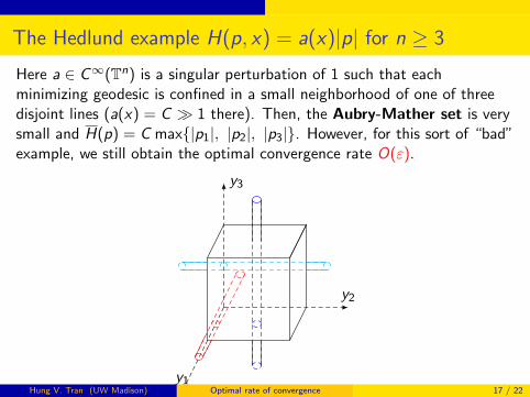
The Hedlund example H(p, x) = a(x)|p| for n ≥ 3
Here a ∈ C∞(Tn) is a singular perturbation of 1 such that eachminimizing geodesic is confined in a small neighborhood of one of threedisjoint lines (a(x) = C � 1 there). Then, the Aubry-Mather set is verysmall and H(p) = C max{|p1|, |p2|, |p3|}. However, for this sort of “bad”example, we still obtain the optimal convergence rate O(ε).
y1
y2
y3
Hung V. Tran (UW Madison) Optimal rate of convergence 17 / 22
Let me just report here two related results.
Theorem (Jing–T.–Yu (2019))
Assume that H(p, x) = a(x)|p| where a ∈ C (Tn, (0,∞)). Let H be thecorresponding effective Hamiltonian. If {p : H(p) ≤ 1} is a centrallysymmetric polytope in Rn, then we have optimal rate of convergence O(ε).
And here is a result (inverse problem type) saying that all centrallysymmetric polytopes with rational coordinates are admissible.
Theorem (Jing–T.–Yu (2019)–generalization of Hedlund’s example)
Assume n ≥ 3. Let P be a centrally symmetric polytope with nonemptyinterior in Rn. Then, there exists a ∈ C∞(Tn, (0,∞)) such that, forH(p, x) = a(x)|p|, the corresponding effective Hamiltonian satisfies{p : H(p) ≤ 1} = P.
Hung V. Tran (UW Madison) Optimal rate of convergence 18 / 22
Some new ideas in the proof of JTY
We consider the reachable set framework. Let Y = [0, 1]n, and{Rt(x) = {y ∈ Rn : γ(0) = x , γ(t) = y , |γ′(s)| ≤ a(γ(s)) a.e. s ∈ [0, t]},Rt(Y ) =
⋃x∈Y Rt(x).
Then, we have the following important observation: For t, s > 0,
Rt+s(Y ) ⊂ Rt(Y ) +Rs(Y ) + (−Y ).
Let Xm = coRm(Y ) + (−Y ) for m ∈ N. Then, Xm is convex, compact,and
Xm+k ⊂ Xm + Xk for all m, k ∈ N.
This is an important subadditive property for a sequence of convex,compact set {Xm}.
Hung V. Tran (UW Madison) Optimal rate of convergence 19 / 22
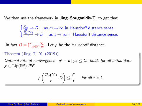
We then use the framework in Jing–Souganidis-T. to get that{Xmm → D as m→∞ in Hausdorff distance sense,Rt(Y )
t → D as t →∞ in Hausdorff distance sense.
In fact D =⋂
m∈NXmm . Let ρ be the Hausdorff distance.
Theorem (Jing–T.–Yu (2019))
Optimal rate of convergence ‖uε − u‖L∞ ≤ Cε holds for all initial datag ∈ Lip(Rn) IFF
ρ
(Rt(Y )
t,D
)≤ C
tfor all t > 1.
Hung V. Tran (UW Madison) Optimal rate of convergence 20 / 22
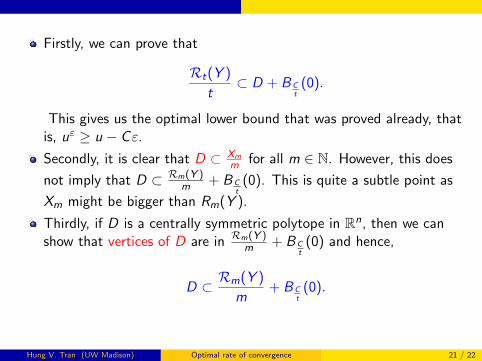
Firstly, we can prove that
Rt(Y )
t⊂ D + BC
t(0).
This gives us the optimal lower bound that was proved already, thatis, uε ≥ u − Cε.
Secondly, it is clear that D ⊂ Xmm for all m ∈ N. However, this does
not imply that D ⊂ Rm(Y )m + BC
t(0). This is quite a subtle point as
Xm might be bigger than Rm(Y ).
Thirdly, if D is a centrally symmetric polytope in Rn, then we canshow that vertices of D are in Rm(Y )
m + BCt
(0) and hence,
D ⊂ Rm(Y )
m+ BC
t(0).
Hung V. Tran (UW Madison) Optimal rate of convergence 21 / 22
Concluding remarks
This is just the beginning. There are many more interesting questions tobe studied.
1 The case where H = H(p, x , xε ) or the case where H = H(p, xε ,tε).
2 Periodic homogenization for static problem uε + H(Duε, x , xε ) = 0.
3 Quasi/Almost periodic setting.
4 Stationary ergodic setting: Improve the result byArmstrong–Cardaliaguet–Souganidis.
THANK YOU FOR YOUR ATTENTION!
Hung V. Tran (UW Madison) Optimal rate of convergence 22 / 22