Convergence-Panel Data 200805

Research Institute of Applied Economics 2008 Working Papers 2008/05, 32 pages

1

Panel Data Stochastic Convergence Analysis of the Mexican Regions

Josep Lluís Carrion-i-SilvestreΩ and Vicente German-SotoΦ. ΩIREA-AQR Group. Departament d’Econometria, Estadística i Economia Espanyola. Universitat de Barcelona. ΦFacultad de Economía, Universidad Autónoma de Coahuila. Unidad Camporredondo Edificio “E”. Planta Baja, C.P. 25280. Saltillo, México

Abstract: The stochastic convergence amongst Mexican Federal entities is analyzed in panel data framework. The joint consideration of cross-section dependence and multiple structural breaks is required to ensure that the statistical inference is based on statistics with good statistical properties. Once these features are accounted for, evidence in favour of stochastic convergence is found. Since stochastic convergence is a necessary, yet insufficient condition for convergence as predicted by economic growth models, the paper also investigates whether β-convergence process has taken place. We found that the Mexican states have followed either heterogeneous convergence patterns or divergence process throughout the analyzed period. Keywords: Stochastic convergence, β-convergence, non-stationarity panel data tests, cross-section dependence, multiple structural breaks. JEL Codes: C12, C22, C32, O40, R11.


2

1. Introduction

Panel data techniques have attracted the attention of most empirical practitioners that pursue

better statistical inference through a combination of the information in both the cross-section

(N) and time (T) dimensions. The increasing availability of statistical information has led to

the application of panel-data-based statistics to sets of countries, sectors, regions or cities. An

interesting feature that advocates the use of panel data techniques is that the time series are

expected to share similar stochastic properties. This characteristic is even more likely to be

found at regional level, where the individuals are exposed to common policies coming from

national governments. If this is the case, taking into account both the cross-section and time

series variation using a panel data approach might lead to an improvement in the statistical

inference.

Macroeconomic panel data sets are characterized by having large time dimension, which

implies that non-stationarity should be taken into account when conducting economic

analyses if meaningful interpretations are to be obtained. This requires that the stochastic

properties of panel data sets have to be assessed. In this regard, recent proposals in the

econometric literature generalize unit root, stationarity and cointegration test statistics to

panel data framework. These proposals differ depending on the degree of individual

heterogeneity that is accommodated, the presence of cross-section dependence among

individuals, and the stability of the parameters of the model, among other features – see, for

instance, Banerjee (1999), Baltagi (2005), and Breitung and Pesaran (2007) for overviews of

the field.

Although economic growth analysis has attracted the interest of many researchers, the studies

that focus on developing countries from a regional point of view using panel data statistics are

scarce. The aim of this paper is to fill this gap and increase the empirical evidence concerning

income convergence for the Mexican regional case. Although there are some studies that deal

with the Mexican regions – see Esquivel (1999), Cermeño (2001), and Carrion-i-Silvestre and

German-Soto (2007) – none of them are based on the joint consideration of exploiting the

information in the panel data set over a long period of time. Therefore and to the best of our

knowledge, this is the first study that analyses the Mexican regional convergence

phenomenon from a non-stationary panel data point of view.


3

Some caution has to be taken when using non-stationary panel data statistics, since some of

the proposals (the so-called first generation panel tests) assume that time series in the panel

data are independent. The lack of consideration of the cross-section dependence might bias

the analysis to conclude in favour of the stationarity of the panel data even in the case where it

is non-stationary – see O’Connell (1998), and Banerjee, Marcellino and Osbat (2004, 2005).

Fortunately, we can test the assumption of cross-section independence using the statistics in

Pesaran (2004) and Ng (2006). In the case that these statistics point to the existence of cross-

section dependence, we will then have to use panel data statistics (the so-called second

generation panel tests).

The paper considers another relevant feature that is present in our data. Previous studies of the

Mexican case – see, for instance, Chiquiar (2005), and Carrion-i-Silvestre and German-Soto

(2007) – have revealed the existence of structural breaks that have affected the individual

GDP in different ways – among the numerous events we can think of are the economic crises

and reforms that took place in the eighties and nineties that so characterize the Mexican

economic growth experience. These events might have changed the relationships of the

economy as well as the convergence trends. It is well known that the presence of unattended

structural breaks can bias the conclusions drawn from the application of unit root and

stationarity statistics, both in univariate and panel data framework, concluding in favour of the

unit root hypothesis – Perron (1989), Lee, Huang and Shin (1997), Montañés and Reyes

(1998), and Carrion-i-Silvestre, del Barrio-Castro and López-Bazo (2002), among others.

Therefore, a tension might appear when using panel data statistics, since unattended cross-

section dependence might bias the analysis towards stationarity, whereas unattended structural

breaks might bias the analysis towards non-stationarity. Consequently, the analysis has to

consider both features. To this end, we compute the statistic in Carrion-i-Silvestre, del Barrio-

Castro and López-Bazo (2005) that accommodates the presence of multiple structural breaks

and cross-section dependence among individuals. The analysis reveals that the joint

consideration of both features points to the existence of stochastic convergence, though only

for some states is β-convergence found.

The paper is organized as follows. Section 2 describes the methods and models that are used

to study the presence of stochastic convergence. Section 3 introduces the econometric

methodology and results of the stochastic convergence analysis amongst Mexican Federal


4

entities. The presence of β-convergence is investigated in Section 4. Section 5 discusses the

main economic implications for regional policies of the results. Finally, Section 6 concludes.

2. Convergence hypothesis and panel-data-based tests: A brief overview

Barro and Sala-i-Martin (1991, 1992) were the first who introduced the notion of β and σ

convergence to assess whether the poor states (or countries) grow faster than the richer ones,

implying that they will catch up (β-convergence) in the long-run, or whether the dispersion of

the income diminishes (σ-convergence) over time. However, the econometric validity of these

cross-section based approaches was questioned by Quah (1993), Carlino and Mills (1993),

Bernard and Durlauf (1995), and Evans (1998), who defend the use of time series methods

given that the cross-section approach is subject to bias (Quah, 1993).

Following Bernard and Durlauf (1995), N economies are said to converge if, and only if, a

common trend at and finite parameters δ1, δ2, …, δN exist so that

( ) ,lim , ittit ay δ=−∞→ (1)

for i = 1,…, N, where yi,t denotes the real per capita income of the i-th time series. In order to

account for the unobservable common trend, we define the average of the N economies so that

( ) ,1lim1∑=

∞→ =−N

iittt N

ay δ (2)

where ∑=

−=N

itit yNy

1,

1 denotes the average per capita GDP – the benchmark time series. If we

define the level of the common trend so that ( ) 0lim =−∞→ ttt ay , and subtracting (2) from (1),

stochastic convergence exists if, and only if,

( ) .lim , ittit yy δ=−∞→ (3)

In this framework, convergence is said to be absolute if, and only if, the unconditional mean

δi = 0 in (3), while convergence is said to be conditional when δi ≠ 0 in (3). Bernard and

Durlauf (1995) state that stochastic convergence occurs when per capita income of one

economy relative to the benchmark economy is stationary, so we are therefore close to the

steady-state. In this regard, stochastic convergence implies that idiosyncratic regional-specific

factors cannot explain long-run economic growth and, moreover, that shocks to relative real


5

per capita GDP have temporary effects. Thus, stochastic convergence implies that differences

across economies are not persistent, and long-run movements in regional GDP are driven by

common technology shocks (Evans, 1998).

In order to capture deviations from relative trend growth, Carlino and Mills (1993) propose to

model deviations from the equilibrium (δi) as the combination of a time trend and a stochastic

process: δi = μi + β i t + ui . (4)

Therefore, regional output (yi,t) is said to converge to the average of regional per capita output

( ty ) if ( )tti yy −, is stationary. As pointed out in Carlino and Mills (1993), the specification

given by (4) is a dynamic version of the Baumol hypothesis. Thus, β-convergence requires

that if a region is initially above its compensating differential (μi), it should grow more slowly

than the benchmark, which implies βi < 0 in (4). On the other hand, if the region is initially

below its compensating differential, then βi > 0 in (4).

It is worth mentioning that although there are other approaches in the literature to analyze the

presence of convergence – for instance, Quah (1996) studies the dynamic of the distribution,

whereas Phillips and Sul (2007) use a non-linear factor model – in this paper we follow the

approach in Carlino and Mills (1993), which relies on the application of unit root and

stationarity statistics.

Empirical evidence based on univariate unit root and stationarity tests is not conclusive. Some

papers often find convergence, while others conclude that GDP differentials persist and,

therefore, economies diverge. On the one hand, Evans and Karras (1996) and Evans (1997)

find stochastic convergence for the contiguous US states from 1929 to 1991, as well as for 54

countries using the Summers and Heston database from 1950 to 1990. On the other hand, Lee,

Pesaran and Smith (1997) conduct convergence tests and find that steady-state growth rates

differ substantially between the economies of 102 countries between 1960 and 1989. Some

authors have argued that the lack of finding stochastic convergence may be driven either by

the low power of univariate tests and/or by misspecification errors caused by unattended

structural breaks. This has given rise to new analyses that consider either the presence of

structural breaks on a country-by-country basis or the use of panel data statistics to increase

the empirical power of unit root tests.


6

Country-by-country analysis considering the presence of structural breaks can be found in

Loewy and Papell (1996), and Tomljanovich and Vogelsang (2002), who confirm the

evidence of convergence obtained in Carlino and Mills (1993) for the US regions. Smyth and

Inder (2004) for the Chinese regions, DeJuan and Tomljanovich (2005), and Rodríguez

(2006) for the Canadian regions, and Strazicich, Lee and Day (2004), and Dawson and Sen

(2007) for some OECD countries, and Carrion-i-Silvestre and German-Soto (2007) for the

Mexican regions, are some additional examples in the literature where the inclusion of

structural breaks favours the finding of convergence.

Recently, panel-data-based unit root tests have been used to conduct stochastic convergence

analysis. Fleissig and Strauss (2001) use panel data unit root tests concluding that real per

capita GDP for OECD countries and one European sub sample converge in the period 1948-

1987, but not in the entire sample of 1900-1987. Note that the fact of not accounting for the

presence of structural breaks might be the reason why stochastic convergence is not

encountered when focusing on the whole period. A similar situation is found in Pedroni and

Yao (2006) for the Chinese regions, who conduct the analysis using panel data unit root tests

with the definition of two sub samples. Pedroni and Yao (2006) conclude that there has been

stochastic convergence for the 1978’s Chinese pre-reform period, but not for the post-reform

period.

Existing evidence that is based on the use of panel data unit root tests does not explicitly

consider the presence of structural breaks, although previous analyses indicate that structural

breaks might be affecting the time series that cover long periods. Therefore, the empirical

approach that we undertake in this paper can be seen as a novelty that will prompt the

development of further empirical analyses for other countries.

3. Econometric methodology and results

In order to investigate the presence of stochastic convergence amongst Mexican regions we

compute panel-data-based unit root and stationarity statistics. We apply the panel data unit

root based tests in Maddala and Wu (1999) – hereafter MW – and Im, Pesaran and Shin


7

(2003) – henceforth IPS – as well as the panel data stationarity tests in Hadri (2000), which

are suitable for panel data sets with moderate N compared to T. The analysis tests the cross-

section independence hypothesis that is assumed in all these panel data statistics. When this

hypothesis is not satisfied, further statistics have to be computed to take account of the effects

of cross-section dependence. Finally, we also consider the presence of multiple structural

breaks, which is to be expected in our case given the previous studies in the literature that

focus on the Mexican regional case.

The data set is the annual real per capita GDP for the N = 32 Mexican regions during the

period 1940-2001. Annual real GDP data set is provided in German-Soto (2005) and

population data comes from INEGI (1999). We have investigated the presence of convergence

using the difference between the logarithm of per capita real GDP in the Mexican regions (yi,t,

i = 1,…,N) and the logarithm of the national per capita real GDP (yt). Figure 1 depicts those

relative income differences.

-- Insert Figure 1 here --

3.1. Panel data unit root and stationary statistics

The test in Im, Pesaran and Shin (2003) is based on the estimation of:

( ) ,,*,,

1

*1,

*, tiktiki

p

ktiiiti yytfy εγδ +Δ++=Δ −

=− ∑

(5)

where throughout the paper ( )ttiti yyy −= ,*, denotes the difference (in logarithms) between

regional and national real per capita income, fi(t) denotes the deterministic component and εi,t

is assumed to be independently distributed across i and t, i = 1,..., N, t = 1,..., T. It is worth

noticing that throughout the paper we consider the deterministic specification that includes a

linear time trend, since this specification is consistent with the definition of convergence as

given in Carlino and Mills (1993). The null hypothesis is given by Ho: δi = 0, ∀i, whereas the

alternative hypothesis H1: δi < 0 for at least one i. Im, Pesaran and Shin (2003) propose the

standardised group-mean Lagrange Multiplier (LM) bar test statistic – denoted as LMΨ – and

the standardised group-mean t bar test statistic – denoted as tΨ – to test the null hypothesis of

panel data unit root, which are shown to converge to the standard Normal distribution.

Besides, Maddala and Wu (1999) propose combining the individual p-values (πi) associated


8

with the pseudo t-ratio for testing δi = 0 in (5). The test is given by MW ( )iNi πln2 1∑−= = ,

which under the null hypothesis is distributed according to MW 22Nχ∼ .1

Evidence of panel data unit root tests can be complemented with the computation of

stationarity tests. In this concern, Hadri (2000) provides a panel statistic where the null

hypothesis is stationarity. The test in Hadri (2000) assumes that the individual time series *,tiy

is generated according to the following unobserved component model:

( ) titiiti rtfy ,,*, ε++= (6)

,,1,, tititi urr += −

where fi(t) can be either a constant or a linear time trend, εi,t is assumed to be a stationary

process and ui,t ~ iid(0, 2,iuσ ) ∀i, i = 1, …, N, with εi,t and ui,t being mutually independent. In

order to test the null hypothesis of stationarity Hadri (2000) proposes using the panel version

of the test in Kwiatkowski, Phillips, Schmidt and Shin (1992) applied in the univariate context

– hereafter KPSS test. In its heterogeneous version, the test statistic is given by:

,ˆ 2,

1

22

1

1⎟⎟⎠

⎞⎜⎜⎝

⎛= ∑∑

=

−−

=

−ti

T

ti

N

ik STN ωη

(7)

k = μ,τ, where jitjtiS ,1, ε∑= = denotes the partial sum process obtained from the estimated

OLS residuals when regressing the individual time series on a constant – ημ test – or on a time

trend – ητ test. Under the null hypothesis of stationarity, Hadri (2000) shows that the

standardized test statistic given in (7) converges to the standard Normal distribution. We

define 2ˆ iω as a consistent estimate of the long-run variance of εi,t, 2,

12 lim TiTi ST −∞→=ω , i = 1,

…, N. Note that the specification in (7) assumes heterogeneous long-run variances across

individuals, although it is possible to impose homogeneity replacing 2ˆ iω in (7) by

1 In order to facilitate computation of πi we have carried out 100,000 replications to obtain the empirical

percentiles for the ADF test for a DGP given by a random walk without drift. Then a response surface has been

estimated to approximate the corresponding p-values using the logistic functional form given by:

,

exp1exp

ββ

πi

ii z

z+

=

where 44

33

2210 iiiii xxxxz ββββββ ++++= , with xi being the value of the ADF test and πi the

corresponding percentile.


9

21

12 ˆˆ iNiN ωω ∑= =

− . Carrion-i-Silvestre and Sansó (2006) compare different ways to estimate

2iω and suggest using the procedure described in Sul, Phillips and Choi (2005).

Results concerning the IPS, MW and Hadri statistics are reported in Table 1. Panel A in Table

1 offers the statistics that have been computed assuming that the individuals are cross-section

independent. As can be seen, apparently contradictory conclusions are obtained from these

statistics since, in general, the panel data unit root IPS and MW statistics allow the null

hypothesis of unit root to be rejected, while the Hadri’ statistics reject the null of stationarity.

However, we have to bear in mind that rejection of the respective null hypotheses only means

that some of the individuals are either stationary (in the case of the panel unit root tests) or

non-stationary (in the case of the panel stationarity test). Furthermore, this inference is

conditional to the fulfilment of the cross-section independence assumption, which can be

tested using the developments in Pesaran (2004) and Ng (2006).

-- Insert Table 1 here --

3.2. Testing the cross-section independence

Pesaran (2004) designs a test statistic based on the average of pair-wise Pearson’s correlation

coefficients jp , j =1, …, n, n = N(N-1)/2, of the residuals obtained from ADF-type regression

equations – this aims to isolate autocorrelation from cross-section dependence. The CD

statistic in Pesaran (2004) that tests the null hypothesis of cross-section independence against

the alternative of dependence is given by

( ).1,0~ˆ2

1

NpnTCD

n

jj∑

=

=

The approach in Ng (2006) relies on the computation of spacings to test the null hypothesis of

independence. In brief, the procedure in Ng (2006) works as follows. First, we get rid of

autocorrelation pattern in individual time series through the estimation of ADF-type

regression equations. As for the test in Pesaran (2004), this allows us to isolate cross-section

regression from serial correlation. Taking the estimated residuals from the ADF-type

regression equations, we compute the absolute value of Pearson’s correlation coefficients

( )jj pp ˆ= for all possible pairs of individuals, j =1, …, n, where n = N(N-1)/2, and sort them

in ascending order. As a result, we obtain the sequence of ordered statistics given by


10

[ ] [ ] [ ] nnnn ppp ::2:1 ,,, K . Under the null hypothesis that 0=jp and assuming that individual

time series are Normal distributed, jp is half-normally distributed. Furthermore, let us define

jφ as [ ]( )njpT :Φ , where Φ denotes the cdf of the standard Normal distribution, so that

( )nφφφ ,,1 K= . Finally, let us define the spacings as 1−−=Δ jjj φφφ , j =1, …, n.

In addition, Ng (2006) proposes splitting the whole sample (W) of (ordered) spacings at

arbitrary ( )1,0∈ϑ , so that we can define the group of small (S) correlation coefficients and

the group of large (L) correlation coefficients. The definition of the partition is carried out

through the minimization of the sum of squared residuals

( )[ ]

( )( )[ ]

( )( ) ,2

1

2

1

ϑφϑφϑϑ

ϑ

Lj

n

njSj

n

jnQ Δ−Δ+Δ−Δ= ∑∑

+==

where ( )ϑSΔ and ( )ϑLΔ denotes the mean of the spacings for each group respectively.

Consistent estimate of the break point is obtained as ( ) ( )ϑϑ ϑ nQ1,0minargˆ∈= , where definition

of some trimming is required – we follow Ng (2006) and set the trimming at 0.10. Once the

sample has been split, we can proceed to test the null hypothesis of independence in both sub

samples. Obviously, the rejection of the null hypothesis for the small correlations sample will

imply also rejection for the large correlations sample as the statistics are sorted in ascending

order. Therefore, the null hypothesis can be tested for the small, large and the whole sample

using the standardized Spacing Variance Ratio (SVR) in Ng (2006), which under the null

hypothesis of independence converges to the standard Normal distribution.

The computation of the Pesaran’s (2004) CD statistic gives CD = 14.316, which strongly

rejects the null hypothesis of cross-section independence when compared to the standard

Normal distribution.2 The same conclusion is reached by the application of Ng’s (2006)

statistic for the whole sample (7.800), for the small sample (6.301) and for the large sample

(6.337). Furthermore, the feature that the SVR statistic points to the existence of cross-section

dependence when looking at the whole sample and both sub samples can be interpreted as an

indication that cross-section dependence is pervasive, a feature that can be accommodated by

the specification of approximate factor model such as those in Bai and Ng (2004). These

2 In order to isolate the correlation, we estimate an ADF-type regression equation where the order of the model is selected using the Ng and Perron (1995) t-sig criterion with up to ten lags.


11

elements indicate that panel data unit root and stationarity tests have to account for the

presence of cross-section dependence.

3.3. Panel data statistics with cross-section dependence

Earlier proposals in the literature addressed the presence of cross-section dependence either

including temporal effects (cross-section demeaning) – see Levin, Lin and Chu (2002), and

Im, Pesaran and Shin (2003) – or through the computation of the empirical distribution by

means of parametric Bootstrap – see Maddala and Wu (1999) for further details. In this paper

we follow these two approaches and compute (i) the IPS, MW and Hadri statistics for the

cross-section demeaned data, and (ii) the empirical Bootstrap distribution for the IPS, MW

and Hadri statistics.

Recent developments have included the presence of the cross-section dependence in the

model through the specification of approximate factor models – see Bai and Ng (2004), Moon

and Perron (2004), and Pesaran (2007), among others. Since the proposal in Bai and Ng

(2004) is the most general one, we compute here their statistics. The Bai and Ng (2004)

approach decomposes the observable variables as follows

( ) ,,*, tiititi eFtfy ++= ′ξ

t = 1, …, T, i = 1, …, N , where fi(t) denotes the deterministic part of the model – either a

constant or a linear time trend – Ft is a (r x 1)-vector that accounts for the common factors

that are present in the panel, and ei,t is the idiosyncratic disturbance term, which is assumed to

be cross-section independent. Unobserved common factors and idiosyncratic disturbance

terms are estimated using principal components on the first difference model. The panel data

unit root hypothesis on tie ,~ can be tested using the idiosyncratic ADF statistic pooling the

individual p-values. When the estimated number of common factors is 1ˆ =r , we can test the

null hypothesis of unit root on tF using the usual ADF statistic. Finally, when 1ˆ >r we can

use either the parametric or non-parametric MQ statistics suggested in Bai and Ng (2004) to

estimate the number of common stochastic trends. The estimation of the number of common

factors is obtained using the panel BIC information criterion in Bai and Ng (2002).


12

Panel B in Table 1 presents the statistics for the cross-section demeaned panel data set. As can

be seen, previous conclusions are unchanged since the null hypotheses of the IPS, MW and

Hadri’ statistics are strongly rejected. However, it is worth noticing that cross-section

demeaning implies that cross-section dependence is driven by only one stationary common

factor that has the same effect on all individuals. This situation is quite restrictive in practice,

so that other ways to control for the presence of cross-section dependence have to be essayed.

One alternative way to deal with cross-section dependence is the computation of the empirical

distribution using Bootstrap techniques. Panel C in Table 1 reports the critical values for the

statistics presented in Panel A of Table 1 – note that the null hypothesis is tested using the left

tail for the tΨ statistic, and the right tail for the other statistics. Using these critical values, we

conclude that the null hypothesis of non-stationarity cannot be rejected at the 5% level of

significance for the IPS and MW statistics, while the null hypothesis of stationarity is strongly

rejected with the Hadri’ statistics. Therefore, these statistics lead to concluding against the

existence of stochastic convergence.

This conclusion is reinforced when we model the cross-section dependence using the common

factor approach in Bai and Ng (2004). Table 2 shows the panel data statistic that combines the

individual ADF statistics for the idiosyncratic disturbance terms, as well as the MQ tests for

the common factors with the specification of up to six common factors. Using these statistics

we conclude that the null hypothesis of unit root cannot be rejected for the idiosyncratic

disturbances. Furthermore, the MQ tests, either the parametric and non-parametric versions,

point to the presence of six non-stationary common factors. It is worth noticing that the

number of common factors, which has been estimated by the panel Bayesian information

criterion (BIC) in Bai and Ng (2002), coincides with the maximum number of factors that is

permitted – we have increased the maximum number of common factors, but it is achieved as

well. This feature can be understood as evidence of unattended non-stationarity, being the

presence of multiple structural changes a potential source.

-- Insert Table 2 here --

In all, the statistics that consider the presence of cross-section dependence in a general way

indicate that stochastic convergence has not been taking place among the Mexican states

during the analysed time period. However, this conclusion is not robust against the existence


13

of multiple structural breaks, a feature that seems to be present in the data if we rely on

previous analysis in the literature.

3.4. Panel data statistics with multiple structural breaks

We suggest the application of the statistic in Carrion-i-Silvestre, del Barrio-Castro and López-

Bazo (2005), who extend the proposal in Hadri (2000) with the specification of the following

deterministic component:

( ) ,,,,1

,,,1

∗

==∑∑ +++= tkiki

m

kitkiki

m

kii DTtDUtf

ii

γβθα (8)

where 1,, =tkiDU for ikbTt ,> and 0 elsewhere, i

kbkti TtDT ,,, −=∗ for ikbTt ,> and 0 elsewhere,

with TT ii

kb λ=, being the k-th break point for the i-th individual, k = 1, …, mi, and i = 1, …,

N, and )1,0(∈iλ denoting the relative position of the structural breaks (break fraction) for the

i-th individual. The null hypothesis of stationarity is tested using the standardized statistic in

(7), where the partial sum process is computed from the OLS residuals that are obtained using

(8) – hereafter the panel statistic in Carrion-i-Silvestre, del Barrio-Castro and López-Bazo

(2005) is denoted by Z(λ), where )',,( ''1 Nλλλ K= collects the break fractions for all

individuals. As can be seen, the deterministic specification given by (8) accounts for the

presence of multiple structural breaks that affect either the level and/or the trend of the time

series. In order to estimate the break points, Carrion-i-Silvestre, del Barrio-Castro and López-

Bazo (2005) suggest applying the procedure first proposed in Bai and Perron (1998). The

presence of cross-section dependence can be accounted for, either by cross-section demeaning

or computing the empirical distribution by means of Bootstrap techniques.

3.4.1. Break point estimation

Provided that the variables that we are analysing show trending behaviour, the number of

structural breaks have been selected using the modified Bayesian information criterion

defined in Liu, Wu and Zideck (1997). The initial maximum number of structural breaks that

we allow in our set-up is mmax = 3. However, in some cases this maximum is achieved, so that

in order to ensure that there are no structural breaks left we increase mmax sequentially to mmax

= 5 or mmax = 8, depending on whether the maximum given by mmax is achieved. This

sequential re-specification of the maximum number of structural breaks is adopted because


14

the precision of the break point estimation drawn from the procedure in Bai and Perron (1998)

depends on mmax, i.e., the less mmax, the more information is used to estimate the break points.

Therefore, the increase of mmax and the consequent reduction in the amount of information

that is used to estimate the break points can be understood as the price that we have to pay in

order to ensure that we control for all possible structural breaks affecting each individual.

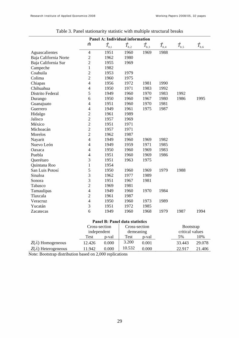
-- Insert Table 3 here –

Panel A in Table 3 presents the estimated number ( m ) and position of the break points for

each relative regional per capita income. The procedure detects one break for two individuals,

two breaks for eleven individuals, three breaks in four cases, four breaks for eleven

individuals, five breaks in two cases and, finally, six breaks in two cases. As can be seen,

there is a high heterogeneity in the number and position of the break points among

individuals.

Some estimated break points seem to respond to diverse events that affected either the whole

Mexican economic activity (economic crises and reforms) or the economy of each Mexican

region. For example, eleven of the detected break points are located around the crises of 1976,

1982, 1987 and 1994/1995, while three structural breaks are estimated in the period of the

Mexican oil boom (between 1975 and 1986). Also, break points between 1982 and 1989

correspond to a convulse stage of the Mexican economy (high rates of inflation,

unemployment and null rates of growth). Meanwhile, dates located before 1975 correspond to

a stage of quick reduction of the per capita income differences.

We can carry out a more detailed analysis focusing on some of the Mexican states. For

example, the estimates report only one break point for Quintana Roo. According to the

estimated coefficients, Quintana Roo’s real per capita income was converging from above to

the national one in 1954, although from then on it has converged from below. Technically, the

constant term fell to lower levels in that year. This result could be a consequence of mixed

events. First, national GDP recorded an important increase (of about 10%) in 1954 and,

second, the tourism sector, which is Quintana Roo’s main sector of economic activity,


15

suffered an important income reduction in this period. As a consequence, Quintana Roo’s

relative income fell importantly. The Mexican oil boom, which occurred between 1975 and

1983, is also captured by the model. Campeche, Chiapas and Tabasco are the main oil

producers of Mexico and the procedure has selected 1982, 1981 and 1981, respectively, as

break points for these states. Data from the economic census of Mexico indicate than in those

years oil production tripled.3

Four border states (Chihuahua, Nuevo León, Sonora and Tamaulipas) exhibited convergence

from above and the other two border states (Baja California and Coahuila) exhibited

divergence from above until their respective break point located in the eighties. After that, all

border states (except Tamaulipas) diverge from above. This fact indicates that Border states

have reaped most of the benefits from the trade reforms – after 1985 they exhibited an

increasing tendency in their share of overall manufacturing employment, from 21% in 1985 to

34% in 1998. Five break points are estimated for Distrito Federal (1949, 1960, 1970, 1983

and 1992). Up to 1983 Distrito Federal exhibited a uniform process of convergence from

above, during 1983-1992 this state converged from below, and after 1992 the entity diverges

from above. In this case we can see that in the period 1980-1988 the Mexico City region’s

share of manufacturing employment fell from 44.4% to 33.2%, as a consequence of

decentralization policies aimed to diminish over-population in the capital and the metropolitan

area.

For the Southern states of Chiapas, Guerrero, Oaxaca, and Puebla we have estimated negative

coefficients after their break points in 1990, 1987, 1983, and 1986, respectively. For these

years one characteristic linking this group of states is found in their agricultural sector.

Between 1984 and 1992 the prices of coffee and cocoa declined by more than 70% on

international markets, primarily as a result of the dismantling of the International Coffee

Agreement. It is estimated that subsistence income for small farmers in the Southern states of

the Pacific Coast declined an average of 15% and that indigenous producers were one of the

groups most severely affected by the decline in the price of coffee – as 65% of all coffee

producers are indigenous and produce one-third of Mexico’s coffee output. Furthermore, this

3 Data from INEGI (1999) points out that in 1975 were extracting 261,589 (in thousands) barrels of oil, while in 1982 this quantity ascended to 1,002, 436 (also in thousands).


16

is consistent with the finding that poverty incidence increased very sharply between 1984 and

1994 in the South of the country.

3.4.2. Panel data statistics results

Before proceeding to compute the panel statistic that combines the individual information, we

have to assess whether time series are cross-section independent. As before, we base our

inference on the Pesaran (2004) and Ng (2006) statistics. In order to isolate the correlation

from the dependence issue, we have estimated an ADF-type regression equation that includes

the dummy variables to capture the presence of the structural breaks estimated previously

with up to five lags for the order of the autoregressive model. The order of the model is

selected using the Ng and Perron (1995) t-sig criterion. The residuals from these regressions

are used to compute the CD statistic, which takes the value of CD = 7.269 and, hence, when

compared with the standard Normal distribution leads to a rejection of the null hypothesis of

independence. This conclusion is also found by Ng’s (2006) statistic both for the whole

sample (5.202) and the large sample (4.004), although the null hypothesis of independence

cannot be rejected at the 5% level of significance for the small sample (1.291). Given that the

proportion of statistics in the small group ( 4334.0ˆ =θ ) is smaller than the one for the large

group, together with the result obtained by the CD test, we can conclude that there is

significant evidence of cross-section dependence. As mentioned above, this invalidates the

inference drawn from the panel data statistics that assume cross-section independence – Table

3 offers these statistics for completeness.

Let us focus on the results that control for the presence of cross-section dependence. As the

first approximation, we have proceeded to remove the cross-section mean to the individual

time series and then computed the panel data statistic in Carrion-i-Silvestre, del Barrio-Castro

and López-Bazo (2005). The results are reported in Panel B of Table 3, which indicate that

the null hypothesis of stationarity is strongly rejected by both the homogeneous and

heterogeneous long-run variance versions of the statistic. However, we should bear in mind

that this approximation to remove the cross-section dependence is restrictive, so that other

general ways to consider the cross-section dependence are essayed. In this regard, we have

computed the empirical distribution of the statistic by Bootstrap techniques. Panel B in Table

3 offers the Bootstrap critical values. Note that if we compare the value of the Z(λ) statistic,


17

either computed using homogeneous (Z(λ) = 12.426) or heterogeneous (Z(λ) = 11.942) long-

run variance, with the Bootstrap critical values the null hypothesis of stationarity cannot be

rejected at the 5% level of significance.

To sum up, after the analysis has been controlled for the presence of multiple structural breaks

and cross-section dependence, the results that have been obtained indicate that relative

regional Mexican per capita incomes show stationary fluctuations around a broken trend, i.e.,

the study has found evidence of stochastic convergence. However, this sole evidence does not

warrant the existence of convergence, since according to Carlino and Mills (1993) and

Tomljanovich and Vogelsang (2002), actual convergence exists if stochastic convergence and

β-convergence are verified.

4. The analysis of β-convergence

Our previous findings support the presence of stochastic convergence, a necessary, but not

sufficient, condition to satisfy the definition of β-convergence. To do so, we follow

Tomljanovich and Vogelsang (2002) and estimate the following equations for all the

individuals:

,,*

,,,

1

1,,,

1

1

*, titkiki

m

ktkiki

m

kti uDTDUy

ii

++= ∑∑+

=

+

=

γθ

where now we define the regressors in an orthogonal way as 1,, =tkiDU and ikbtki TtDT 1,

*,, −−=

for ikb

ikb TtT ,1, ≤<− and 0 elsewhere, with i

kbT , denoting the k-th previously estimated break

point for the i-th individual, k = 1, …, mi, with the convention that 00, =ibT and TT i

mb i=+1, ,

and i = 1, …, N.

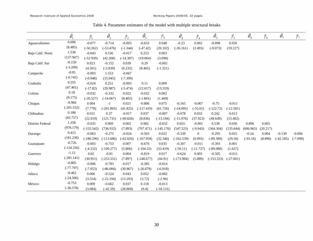
Table 4 reports the estimated coefficients for each of the mi + 1 regimes, along with the

corresponding statistics of significance computed using the Newey and West (1994) robust

estimator of the covariance matrix. Looking at these estimates we can conclude that there has

been β-convergence when the coefficients of the parameters of each regime are significant at

least at the 10% level of significance and have opposite sign, i.e., either when θi,k < 0 and γi,k

> 0, or when θi,k > 0 and γi,k < 0 – using the notation in Tomljanovich and Vogelsang (2002),


18

this situation is denoted as C. Similarly, we conclude that divergence has occurred when the

coefficients of the parameters of each regime are statistically significant at least at the 10%

level of significance and have the same sign, which is denoted in Tomljanovich and

Vogelsang (2002) as D. It is possible to distinguish other interesting situations. Firstly, it

would be possible that one of the parameters of the regime is not significant at the 10% level,

but the other one is. In this case, we use c to denote regimes consistent with β-convergence,

but where only one of the two coefficients is statistically significant at the 10% level of

significance. Similarly, we use d to denote regimes consistent with divergence, but where

only one of the two coefficients is statistically significant at the 10% level of significance.

Secondly, Tomljanovich and Vogelsang (2002) characterize the situation in which both

parameters are non-significant as the case where β-convergence has occurred so that we have

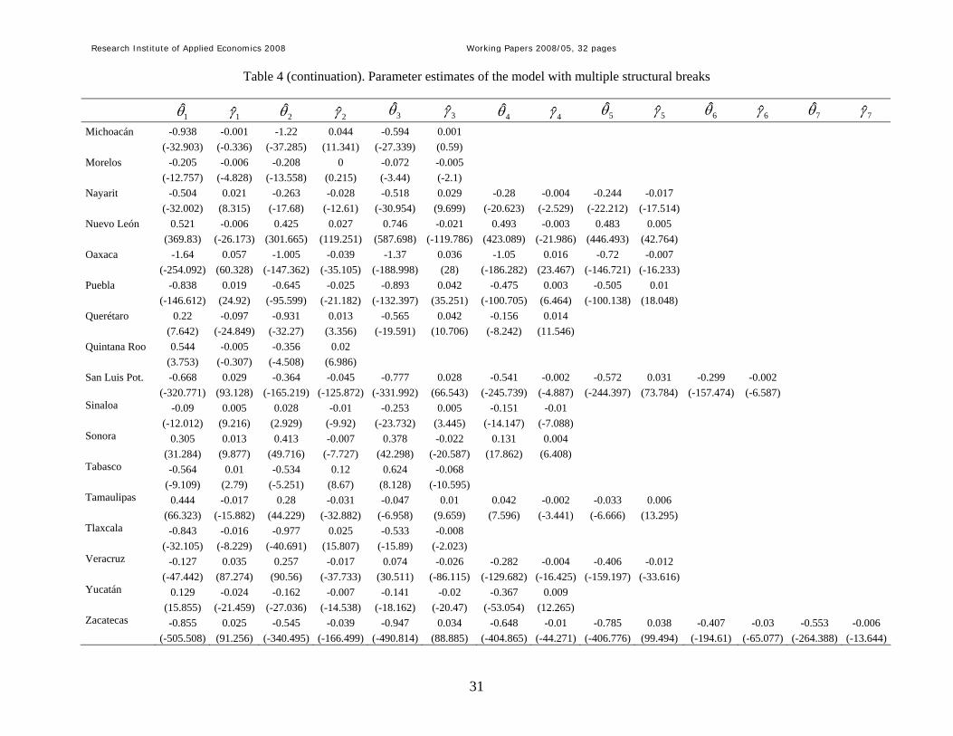
achieved the equilibrium growth. This case is denoted by E. Table 5 summarizes the different

situations corresponding to each regime. Note that Table 5 presents whether the states

converge for different regimes, although the precise definition of these regimes has to be done

using the information in Table 3. For instance, the first regime for Aguascalientes covers from

1940 till 1951, while the one for Baja California Norte goes from 1940 till 1962. The second

regime for Aguascalientes goes from 1952 till 1960, while for Baja California Norte goes

from 1963 till 1980.

-- Insert Tables 4 and 5 here --

In general, estimates suggest that β-convergence has taken part during the analysed period,

although the process of convergence has not been uniform in all cases. For the first regime

there was divergence in seven states (Chihuahua, Guanajuato, Hidalgo, Michoacán, Morelos,

Sonora and Tlaxcala), equilibrium growth for one state (Campeche), and a β-convergence

process in twenty-four out of the thirty-two states. For the last regime, β-convergence has

only been achieved for Colima, eighteen states are consistent with divergence (Baja California

N., Coahuila, Chiapas, Chihuahua, Distrito Federal, Durango, Guerrero, Hidalgo, Morelos,

Nayarit, Nuevo León, Oaxaca, San Luis Potosí, Sinaloa, Sonora, Tlaxcala, Veracruz and

Zacatecas), and only for thirteen states β-convergence is occurring. A similar analysis

indicates that most of the convergence was achieved in the 1980s.4 Comparatively, for the

4 The analysis is based in the prevalent regime at the beginning of the 80s.


19

regimes in the 1980s we observe more states in equilibrium growth (2 to 1), less states in

divergence (9 to 18) and more states in a convergence process (21 to 13) than the last regime.5

Figure 2 reflects this situation.

--Insert Figure 2 here –

Figure 2 suggests that border states were approaching the national income from above, while

southern states were approaching from below in the 1980s. Results in this period widely

contrast with those obtained in the first and last regimes, where some border states showed

divergence from above and some southern states showed divergence from below. Figure 2

also highlights that all states that diverge from above to the national income are regions with

high income levels (they are Sonora and Chihuahua, in the first regime, and Baja California

N., Coahuila, Chihuahua, Distrito Federal, Nuevo León and Sonora, in the last regime), while

nearly all of the states that diverge from below are regions with lower income levels (for

example Hidalgo, Michoacán, Morelos and Tlaxcala, in the first regime, and Chiapas,

Guerrero, Oaxaca and Tlaxcala, in the last regime). It suggests that only some of the relatively

richer states had built the structure to take advantage of the new sources of growth derived

from the enhanced opportunities to trade.

5. Economic implications of the results

Mexican regional income inequality is increasingly turning into a major political and social

problem, which is basically manifested in two forms. First, relative economic stagnation,

mainly in the South, makes it difficult for theses states to generate employment activities

resulting in surplus labour migrating to the Centre and Northern states. This transient

population is now seen as the source of a growing social problem. Second, Mexican

experience suggests that trade policy plays an important role in determining regional

economic fortunes. Therefore, if a reduction in inequality is a policy goal, then market

reforms should, at least, have a regional perspective. Results indicate that major attention

from the government to disadvantaged sectors or regions is required, so that income

disparities can be reduced. Thus, note that interregional disequilibrium has not disappeared in

5 The periods of each regime can be different amongst states. So, the analysis shows the evolution of the convergence process in each regime, although it does not imply that all states were converging at the same time.


20

more than twenty years of free market economy. One way to solve this situation is the use of

public investment policies as a redistributive instrument. This is an approach used in the case

of the European regions with excellent results in regional growth and convergence (see, for

example, Meliciani, 2006).

Looking at the results that we have obtained, it is possible to identify general patterns with

important implications for regional policies. In those regions wherever the results suggest that

break points have not been detected in the 1980s and 1990s (Baja California Sur, Coahuila,

Colima, Jalisco, México, Michoacán, Querétaro, and Quintana Roo) the persistence of

macroeconomic shocks would be smaller, so that stabilization policies are expected to be

more effective. Two groups of states can be defined depending on the effects of the break

points detected in the 1980s. First, we find those states – Baja California N., Campeche,

Distrito Federal, Guanajuato, Nuevo León, Sonora, Tabasco, Tamaulipas and Yucatán – that

improved their results after the break, suggesting that there is a continued role for government

policies in addressing their structural problems given the finding of convergence and

divergence from above. Second, we find those states – Chiapas, Guerrero, Hidalgo, Morelos,

Nayarit, Oaxaca, Puebla, San Luis Potosí, Sinaloa, Tamaulipas, Tlaxcala, Veracruz, and

Zacatecas – that worsened their performance after the structural break and for which

macroeconomic policies seem not to be so effective in dealing with sudden shocks to real

output.

Finally, we detect break points in Chiapas, Chihuahua, Distrito Federal, Durango, and

Zacatecas during the 1980s and 1990s. In these cases the estimated break points can be

indicating more sensibility to macroeconomic shocks than for other states.6 This finding

suggests that government policy initiatives designed to promote economic development will

result in changes in the trend until a new large shock occurs.

6. Concluding remarks

In this paper we have investigated the presence of stochastic convergence amongst Mexican

Federal entities using long time series with panel-data based unit root and stationarity tests.

6 Chiapas state is one exception because of the structural break in 1981 corresponding to the oil boom.


21

The statistical evidence was conducted accounting for both the presence of cross-section

dependence amongst panel units and the presence of multiple structural breaks. The paper has

shown that there is strong dependence amongst the Mexican regions. Only after accounting

for both multiple structural breaks and cross-section dependence, the relative per capita

incomes showed stationary fluctuations around broken trend, i.e., stochastic convergence is

found. However, this sole evidence does not warrant the existence of convergence, since,

according to Carlino and Mills (1993) and Tolmjanovich and Vogelsang (2002), actual

convergence exists if stochastic convergence and β-convergence are verified. The analysis of

β-convergence confirmed that this process is occurring, although it has not been uniform in all

cases. Real per capita income of the Mexican regions has been converging since 1940, but

much of the convergence process occurred in the eighties, before the trade reform. From then

on, convergence process has continued, although the intensity has been weaker than in the

previous period.

The results have important implications for regional policies. In this regard, we have found

that regions with high income levels (mostly of the Mexican North) are diverging from above,

while nearly all of the states that diverge from below are regions with the lower income levels

(mostly of the Mexican South). Moreover, after the trade liberalization, the income gap

amongst rich and poor Mexican states is widening, one aspect that is increasingly turning into

a major political and social problem for Mexico.

References

Bai, J. and S. Ng, 2002, Determining the Number of Factors in Approximate Factor Models,

Econometrica, 70, 191-221.

Bai, J. and S. Ng, 2004, A PANIC Attack on Unit Roots and Cointegration, Econometrica, 72,

4, 1127-1177.

Bai, J., and P. Perron, 1998, Estimating and Testing Linear Models with Multiple Structural

Changes, Econometrica, 66, 47-78.

Baltagi, B., 2005, Econometric Analysis of Panel Data. John Wiley & Sons, Third Edition.

Banerjee, A., 1999, Panel Data Unit Roots and Cointegration: An Overview, Oxford Bulletin

of Economics and Statistics, Special issue, 607-629.


22

Banerjee, A., Marcellino, M. and C. Osbat, 2004, Some Cautions on the Use of Panel

Methods for Integrated Series of Macro-Economic Data, Econometrics Journal, 7, 2, 322-340.

Banerjee, A., Marcellino, M. and C. Osbat, 2005, Testing for PPP: Should We Use Panel

Methods?, Empirical Economics, 30, 77-91.

Barro R. and X. Sala-i-Martin, 1991, Convergence across states and regions, Brookings

Papers on Economic Activity, 1, 107-158.

Barro, R. and X. Sala-i-Martin, 1992, Convergence, Journal of Political Economy, 100, 223-

251.

Bernard A. B., and S. N. Durlauf, 1995, Convergence in international output, Journal of

Applied Econometrics, 10, 97-108.

Breitung, J. and M. H. Pesaran, 2007, Unit roots and cointegration in panels”. Forthcoming in

Matyas, L., Sevestre, P., Eds., The Econometrics of Panel Data, Klüver Academic Press.

Carlino G. A. and L. Mills, 1993, Are U.S. regional incomes converging? A time series

analysis, Journal of Monetay Economics, 32, 335-346.

Carrion-i-Silvestre, J. L., and A. Sansó, 2006, A guide to the computation of stationarity tests,

Empirical Economics, 31, 433-448.

Carrion-i-Silvestre, J. L., and V. German-Soto, 2007, Stochastic Convergence amongst

Mexican States, Regional Studies, 41, 531-541.

Carrion-i-Silvestre, J. L., T. del Barrio, and E. López-Bazo, 2005, Breaking the Panels. An

Application to the GDP per Capita, Econometrics Journal, 8, 159-175.

Carrion-i-Silvestre, J. L., T. Del Barrio, and E. López-Bazo, 2002, Level Shifts in a Panel

Data Based Unit Root Test. An Application to the Rate of Unemployment, Doct. Treball num.

E02/79. University of Barcelona. http://www.ub.edu/ ere/ documents/ papers/ 79.pdf.

Cermeño, R., 2001, Decrecimiento y convergencia de los estados mexicanos. Un análisis de

panel, El Trimestre Económico, 68, 603-629.

Chiquiar, D., 2005, Why Mexico’s regional income convergence broke down, Journal of

Development Economics, 77, 257-275.

Dawson, J. W. and A. Sen, 2007, New Evidence on the Convergence of International Income

from a Group of 29 Countries, Empirical Economics, 33, 199-230.


23

DeJuan, J. and M. Tomljanovich, 2005, Income convergence across Canadian provinces in the

20th century: Almost but not quite there, The Annals of Regional Science, 39, 567-592.

Esquivel, G., 1999, Convergencia regional en México, 1940-1995, El Trimestre Económico,

66, 725-761.

Evans, P., 1997, How Fast Do Economies Converge?, Review of Economics and Statistics,

79, 219-225.

Evans, P., 1998, Using Panel Data to Evaluate Growth Theories, International Economics

Review, 39, 295-306.

Evans, P. and G. Karras, 1996, Convergence Revisited, Journal of Monetary Economics, 37,

249-265.

Fleissig A. R. and J. Strauss, 2001, Panel Unit-Root Tests of OECD Stochastic Convergence,

Review of International Economics, 9, 153-163.

German-Soto, V., 2005, Generación del Producto Interno Bruto Mexicano por entidad

federativa, 1940-1992, El Trimestre Económico, 72, 617-653.

Hadri, K., 2000, Testing for Unit Roots in Heterogeneous Panel Data, Econometrics Journal,

3, 148-161.

Im, K., M.H. Pesaran and Y. Shin, 2003, Testing for unit roots in heterogeneous panels,

Journal of Econometrics, 115, 53-74.

INEGI, 1999, Estadísticas históricas de México, INEGI: Aguascalientes.

Kwiatkowski, D., P. C. B. Phillips, P. J. Schmidt, and Y. Shin, 1992, Testing the Null

Hypothesis of Stationarity Against the Alternative of a Unit Root: How Sure are We that

Economic Time Series Have a Unit Root, Journal of Econometrics, 54, 159-178.

Lee, J., C. J. Huang and Y. Shin, 1997, On Stationary Tests in the Presence of Structural

Breaks, Economics Letters, 55, 165-172.

Lee, K., M. H. Pesaran and R. Smith, 1997, Growth and Convergence in a Multi-Country

Empirical Stochastic Solow Model, Journal of Applied Econometrics, 12, 357-392.

Levin, A., C.F. Lin and J. Chu, 2002, Unit root tests in panel data: asymptotic and finite-

sample properties, Journal of Econometrics, 108, 1-24.

Liu, J., S. Wu and J. V. Zidek, 1997, On Segmented Multivariate Regressions, Statistica

Sinica, 7, 497-525.


24

Loewy, M. B. and D. H. Papell, 1996, Are U.S. regional incomes converging? Some further

evidence, Journal of Monetary Economics, 38, 587-598.

Maddala, G. S. and S. Wu, 1999, A Comparative Study of Unit Root Tests with Panel Data

and a New Simple Test, Oxford Bulletin of Economics and Statistics, Special Issue, 61, 631-

652.

Meliciani, V., 2006, Income and Employment Disparities Across European Regions: The

Role of National and Spatial Factors, Regional Studies, 40, 75-91.

Montañés, A. and M. Reyes, 1998, Effect of a shift in the trend function on Dickey-Fuller unit

root tests, Econometric Theory, 14, 355-363.

Moon, H. R. and B. Perron, 2004, Testing for unit root in panels with dynamic factors,

Journal of Econometrics, 122, 81-126.

Newey, W. and K. West, 1994, Automatic Lag Selecion in Covariance Matrix Estimation,

Review of Economic Studies, 61, 631-653.

Ng, S., 2006, Testing Cross-section Correlation in Panel Data Using Spacings, Journal of

Business & Economic Statistics, 24, 12-23.

Ng, S. and P. Perron, 1995, Unit root tests in ARMA models with data dependent methods for

the selection of the truncation lag, Journal of the American Statistical Association, 90, 268-

281.

O’Connell, P., 1998, The overvaluation of purchasing power parity, Journal of International

Economics, 44, 1-19.

Pedroni, P. and J. Y. Yao, 2006, Regional Income Divergence in China, Journal of Asian

Economics, 17, 294-315.

Perron, P., 1989, The Great Crash, the Oil Price Shock and the Unit Root Hypothesis,

Econometrica, 57, 1361-1401.

Pesaran, M. H. 2004, General Diagnostic Tests for Cross Section Dependence in Panels,

Cambridge Working Papers in Economics, No. 435, University of Cambridge, and CESifo

Working Paper Series No. 1229.

Pesaran, M. H., 2007, A Simple Panel Unit Root Test in the Presence of Cross Section

Dependence, Journal of Applied Econometrics, 22, pp. 265-312.


25

Phillips, P. C. B. and Sul, D., 2007, Transition Modelling and Econometric Convergence

Tests, Econometrica, 76, 1771-1855.

Quah, D. T., 1993, Empirical cross-section dynamics in economic growth, European

Economic Review, 37, 426-434.

Quah, D. T., 1996, Convergence empirics across economies with (some) capital mobility,

Journal of Economic Growth,1, 95-124.

Rodríguez, G., 2006, The role of the interprovincial transfers in the β: Further empirical

evidence for Canada, Journal of Economic Studies, 33, 12-29.

Smyth, R. and B. Inder, 2004, Is Chinese Provincial real GDP per capita nonstationary?

Evidence from Multiple Trend Break Unit Root Tests, China Economic Review, 15, 1-24.

Strazicich, M. C., J. Lee and E. Day, 2004, Are incomes converging among OECD countries?

Time series evidence with two structural breaks, Journal of Macroeconomics, 26, 131-145.

Sul D., P. C. B. Phillips and C. Y. Choi, 2005, Prewhitening Bias in HAC Estimation, Oxford

Bulletin of Economics and Statistics, 67, 517-546.

Tomljanovich, M. and T. J. Vogelsang, 2002, Are U.S. Regions Converging? Using New

Econometric Methods to Examine Old Issues, Empirical Economics, 27, 49-62.


26

Figure 1. Relative regional per capita incomes

-0.25

-0.2

-0.15

-0.1

-0.05

0

0.05

0.1

0.15

0.2

0.25

1940

1943

1946

1949

1952

1955

1958

1961

1964

1967

1970

1973

1976

1979

1982

1985

1988

1991

1994

1997

2000

AGS BCN BCS CAM COA COL CHIA CHIHDF DGO GTO GRO HGO JAL MEX MICHMOR NAY NL OAX PUE QUE QROO SLPSIN SON TAB TAM TLA VER YUC ZAC


27

Figure 2. Map of the regional convergence and divergence


28

Table 1. IPS, MW and Hadri panel data statistics Panel A: Assuming

cross-section

independence

Panel B: Removing

cross-section mean

Panel C: Critical values from the

Bootstrap distribution

Test p-val Test p-val 1% 2.5% 5% 10%

tΨ -2.724 0.003 -2.489 0.006 -4.938 -4.110 -3.491 -2.797

LMΨ 2.988 0.001 2.851 0.002 5.443 4.514 3.829 3.058

MW 83.030 0.055 90.372 0.017 139.296 125.542 114.280 103.135Hadri (Homogeneous) 31.741 0.000 30.708 0.000 9.745 8.128 6.458 4.971Hadri (Heterogeneous) 87.158 0.000 66.771 0.000 9.470 7.777 6.459 4.967Note: Bootstrap distribution based on 2,000 replications

Table 2. Panel data unit root tests with common factors using Bai and Ng (2004) approach Test p-val Number of common stochastic trends

(rmax = 6) Idiosyncratic ADF statistic 3.3636 0.999 MQ_test (parametric) -32.996 6 MQ_test (non-parametric) -31.603 6


29

Table 3. Panel stationarity statistic with multiple structural breaks Panel A: Individual information

m 1,bT 2,bT 3,bT 4,bT 5,bT 6,bT

Aguascalientes 4 1951 1960 1969 1988 Baja California Norte 2 1962 1980 Baja California Sur 2 1955 1969 Campeche 1 1982 Coahuila 2 1953 1979 Colima 2 1960 1975 Chiapas 4 1956 1972 1981 1990 Chihuahua 4 1950 1971 1983 1992 Distrito Federal 5 1949 1960 1970 1983 1992 Durango 6 1950 1960 1967 1980 1986 1995 Guanajuato 4 1951 1960 1970 1981 Guerrero 4 1949 1961 1975 1987 Hidalgo 2 1961 1989 Jalisco 2 1957 1969 México 2 1951 1971 Michoacán 2 1957 1971 Morelos 2 1962 1987 Nayarit 4 1949 1960 1969 1982 Nuevo León 4 1949 1959 1971 1985 Oaxaca 4 1950 1960 1969 1983 Puebla 4 1951 1960 1969 1986 Querétaro 3 1951 1963 1975 Quintana Roo 1 1954 San Luis Potosí 5 1950 1960 1969 1979 1988 Sinaloa 3 1962 1977 1989 Sonora 3 1951 1967 1981 Tabasco 2 1969 1981 Tamaulipas 4 1949 1960 1970 1984 Tlaxcala 2 1961 1987 Veracruz 4 1950 1960 1973 1989 Yucatán 3 1951 1972 1985 Zacatecas 6 1949 1960 1968 1979 1987 1994

Panel B: Panel data statistics

Cross-section independent

Cross-section demeaning

Bootstrap critical values

Test p-val Test p-val 5% 10% Z(λ) Homogeneous 12.426 0.000 3.200 0.001 33.443 29.078Z(λ) Heterogeneous 11.942 0.000 10.532 0.000 22.917 21.406

Note: Bootstrap distribution based on 2,000 replications


30

Table 4. Parameter estimates of the model with multiple structural breaks

1θ 1γ 2θ 2γ 3θ 3γ 4θ 4γ 5θ 5γ 6θ 6γ 7θ 7γ

Aguascalientes 0.096 -0.077 -0.714 -0.003 -0.633 0.048 -0.23 0.002 -0.098 0.026 (8.485) (-50.262) (-53.476) (-1.344) (-47.42) (20.102) (-26.161) (2.493) (-9.073) (19.227) Baja Calif. Norte 1.536 -0.043 0.536 -0.017 0.223 0.003 (137.947) (-52.939) (42.208) (-14.387) (19.064) (3.698) Baja Calif. Sur -0.159 0.023 -0.152 0.039 0.29 -0.002 (-3.209) (4.501) (-2.839) (6.232) (8.465) (-1.321) Campeche -0.05 -0.003 1.553 -0.067 (-0.742) (-0.948) (15.045) (-7.399) Coahuila 0.555 -0.024 0.251 -0.003 0.11 0.009 (47.461) (-17.82) (29.987) (-5.474) (12.017) (13.319) Colima 0.18 -0.032 -0.332 0.022 -0.032 0.002 (9.175) (-20.527) (-14.067) (8.402) (-1.841) (1.469) Chiapas -0.966 0.004 -1 0.021 -0.806 0.075 -0.165 -0.067 -0.75 -0.011 (-201.532) (7.778) (-201.805) (41.825) (-117.419) (61.726) (-24.095) (-55.01) (-122.72) (-12.581) Chihuahua 0.186 0.015 0.37 -0.017 0.037 -0.007 -0.078 0.033 0.242 0.013 (42.757) (22.919) (121.731) (-69.826) (8.836) (-13.194) (-15.976) (37.923) (49.649) (15.402) Distrito Federal 1.358 -0.035 0.969 0.002 0.982 -0.032 0.655 -0.001 0.538 0.036 0.896 0.005 (978.179) (-155.542) (736.932) (7.893) (707.471) (-145.176) (547.525) (-9.943) (364.304) (135.644) (606.965) (20.217) Durango 0.415 -0.063 -0.275 -0.024 -0.503 0.022 -0.339 0 -0.295 0.025 -0.24 0.004 -0.139 -0.006 (181.238) (-186.596) (-113.686) (-62.026) (-167.958) (32.346) (-162.539) (0.093) (-89.389) (29.56) (-93.16) (8.896) (-42.185) (-7.098) Guanajuato -0.726 -0.003 -0.753 0.007 -0.676 0.035 -0.307 -0.011 -0.393 0.001 (-124.336) (-4.332) (-109.277) (5.806) (-104.32) (33.419) (-50.11) (-11.727) (-89.088) (1.637) Guerrero -1.12 0.02 -0.91 0.004 -0.819 0.017 -0.624 0.003 -0.505 -0.011 (-281.141) (30.951) (-253.551) (7.897) (-248.677) (44.91) (-173.984) (5.889) (-153.333) (-27.601) Hidalgo -0.805 -0.006 -0.783 0.017 -0.385 -0.014 (-77.797) (-7.053) (-86.084) (30.967) (-26.679) (-6.918) Jalisco -0.463 0.006 -0.524 0.043 0.052 -0.002 (-24.506) (3.554) (-22.194) (13.293) (3.72) (-2.96) México -0.753 0.009 -0.662 0.037 0.118 -0.013 (-36.578) (3.084) (-42.59) (28.869) (9.4) (-18.131)


31

Table 4 (continuation). Parameter estimates of the model with multiple structural breaks

1θ 1γ 2θ 2γ 3θ 3γ 4θ 4γ 5θ 5γ 6θ 6γ 7θ 7γ

Michoacán -0.938 -0.001 -1.22 0.044 -0.594 0.001 (-32.903) (-0.336) (-37.285) (11.341) (-27.339) (0.59) Morelos -0.205 -0.006 -0.208 0 -0.072 -0.005 (-12.757) (-4.828) (-13.558) (0.215) (-3.44) (-2.1) Nayarit -0.504 0.021 -0.263 -0.028 -0.518 0.029 -0.28 -0.004 -0.244 -0.017 (-32.002) (8.315) (-17.68) (-12.61) (-30.954) (9.699) (-20.623) (-2.529) (-22.212) (-17.514) Nuevo León 0.521 -0.006 0.425 0.027 0.746 -0.021 0.493 -0.003 0.483 0.005 (369.83) (-26.173) (301.665) (119.251) (587.698) (-119.786) (423.089) (-21.986) (446.493) (42.764) Oaxaca -1.64 0.057 -1.005 -0.039 -1.37 0.036 -1.05 0.016 -0.72 -0.007 (-254.092) (60.328) (-147.362) (-35.105) (-188.998) (28) (-186.282) (23.467) (-146.721) (-16.233) Puebla -0.838 0.019 -0.645 -0.025 -0.893 0.042 -0.475 0.003 -0.505 0.01 (-146.612) (24.92) (-95.599) (-21.182) (-132.397) (35.251) (-100.705) (6.464) (-100.138) (18.048) Querétaro 0.22 -0.097 -0.931 0.013 -0.565 0.042 -0.156 0.014 (7.642) (-24.849) (-32.27) (3.356) (-19.591) (10.706) (-8.242) (11.546) Quintana Roo 0.544 -0.005 -0.356 0.02 (3.753) (-0.307) (-4.508) (6.986) San Luis Pot. -0.668 0.029 -0.364 -0.045 -0.777 0.028 -0.541 -0.002 -0.572 0.031 -0.299 -0.002 (-320.771) (93.128) (-165.219) (-125.872) (-331.992) (66.543) (-245.739) (-4.887) (-244.397) (73.784) (-157.474) (-6.587) Sinaloa -0.09 0.005 0.028 -0.01 -0.253 0.005 -0.151 -0.01 (-12.012) (9.216) (2.929) (-9.92) (-23.732) (3.445) (-14.147) (-7.088) Sonora 0.305 0.013 0.413 -0.007 0.378 -0.022 0.131 0.004 (31.284) (9.877) (49.716) (-7.727) (42.298) (-20.587) (17.862) (6.408) Tabasco -0.564 0.01 -0.534 0.12 0.624 -0.068 (-9.109) (2.79) (-5.251) (8.67) (8.128) (-10.595) Tamaulipas 0.444 -0.017 0.28 -0.031 -0.047 0.01 0.042 -0.002 -0.033 0.006 (66.323) (-15.882) (44.229) (-32.882) (-6.958) (9.659) (7.596) (-3.441) (-6.666) (13.295) Tlaxcala -0.843 -0.016 -0.977 0.025 -0.533 -0.008 (-32.105) (-8.229) (-40.691) (15.807) (-15.89) (-2.023) Veracruz -0.127 0.035 0.257 -0.017 0.074 -0.026 -0.282 -0.004 -0.406 -0.012 (-47.442) (87.274) (90.56) (-37.733) (30.511) (-86.115) (-129.682) (-16.425) (-159.197) (-33.616) Yucatán 0.129 -0.024 -0.162 -0.007 -0.141 -0.02 -0.367 0.009 (15.855) (-21.459) (-27.036) (-14.538) (-18.162) (-20.47) (-53.054) (12.265) Zacatecas -0.855 0.025 -0.545 -0.039 -0.947 0.034 -0.648 -0.01 -0.785 0.038 -0.407 -0.03 -0.553 -0.006 (-505.508) (91.256) (-340.495) (-166.499) (-490.814) (88.885) (-404.865) (-44.271) (-406.776) (99.494) (-194.61) (-65.077) (-264.388) (-13.644)


32

Table 5. Convergence and divergence classification of the Mexican regions

Regime 1 Regime 2 Regime 3 Regime 4 Regime 5 Regime 6 Regime 7Aguascalientes C c C C C Baja California Norte C C D Baja California Sur C C c Campeche E C Coahuila C C D Colima C C E Chiapas C C C D D Chihuahua D C C C D Distrito Federal C D C C D D Durango C D C c C C D Guanajuato D C C D c Guerrero C C C C D Hidalgo D C D Jalisco C C C México C C C Michoacán d C c Morelos D c D Nayarit C D C D D Nuevo León C D C C D Oaxaca C D C C D Puebla C D C C C Querétaro C C C C Quintana Roo c C San Luis Potosí C D C D C D Sinaloa C C C D Sonora D C C D Tabasco C C C Tamaulipas C C C C C Tlaxcala D C D Veracruz C C C D D Yucatán C D D C Zacatecas C D C D C D D

Convergence-Panel Data 200805

Documents

Transcript of Convergence-Panel Data 200805