ON THE MOTION PLANNING PROBLEM, … · Journal of Dynamical and Control Systems, Vol. 12, No. 3,...

Journal of Dynamical and Control Systems, Vol. 12, No. 3, July 2006, 371–404 ( c©2006)

ON THE MOTION PLANNING PROBLEM, COMPLEXITY,ENTROPY, AND NONHOLONOMIC INTERPOLATION

JEAN-PAUL GAUTHIER and VLADIMIR ZAKALYUKIN

Abstract. We consider the sub-Riemannian motion planning prob-lem defined by a sub-Riemannian metric (the robot and the cost tominimize) and a non-admissible curve to be ε-approximated in thesub-Riemannian sense by a trajectory of the robot. Several notionscharacterize the ε-optimality of the approximation: the “metric com-plexity” MC and the “entropy” E (Kolmogorov–Jean). In this pa-per, we extend our previous results. 1. For generic one-step bracket-generating problems, when the corank is at most 3, the entropy isrelated to the complexity by E = 2πMC. 2. We compute the en-tropy in the special 2-step bracket-generating case, modelling the carplus a single trailer. The ε-minimizing trajectories (solutions of the“ε-nonholonomic interpolation problem”), in certain normal coordi-nates, are given by Euler’s periodic inflexional elastica. 3. Finally,we show that the formula for entropy which is valid up to corank 3changes in a wild case of corank 6: it has to be multiplied by a factorwhich is at most 3/2.

1. Introduction, notation, statement of the problems

A general motion planning problem from robotics is defined by a triple(Δ, g,Γ):

(i) a distribution Δ over Rn of a certain corank p, which represents the

admissible motion (the kinematic constraints) of the robot;(ii) a Riemannian metric g over Δ providing a (sub-Riemannian) met-

ric structure d to measure the length of admissible curves (actuallyrealized by the robot);

(iii) a smooth nonadmissible curve Γ : [0, 1] → Rn which we want to ap-

proximate by an admissible one. In practice, the choice of Γ makesthe robot avoid possible obstacles in R

n.For given dimension n of the ambient space and corank p of the distri-

bution, the set of motion planning problems Σ = (Δ, g,Γ) is denoted by

2000 Mathematics Subject Classification. 53C17, 49J15, 34H05.Key words and phrases. Robotics, Subriemannian geometry.The second author is supported by grants RFBR 050100458 and UR 0401128.

371

1079-2724/06/0700-0371/0 c© 2006 Plenum Publishing Corporation

372 JEAN-PAUL GAUTHIER and VLADIMIR ZAKALYUKIN

S. We endow S with the standard C∞-topology. [Since our problems arealways local around a compact curve Γ, there is no need to control anythingat infinity, and Whitney topology is not used].

Remark 1. Sometimes, we will impose extra assumptions (e.g., assumingthat distribution is one-step bracket generating). We will still keep thenotation S for the relevant smaller open set of motion planning problems.Assuming that the problem is real analytic, we restrict the C∞-topology tothe subset of analytic objects.

We are interested in approximating or interpolating the curve Γ by ad-missible curves, ε-close (in the sub-Riemannian sense), and we want toanalyze what happens as ε tends to zero (or at least is very small). Thiscorresponds to the practical situation of an ambient space R

n almost full ofobstacles.

We will need “equivalents” of quantities as ε tends to zero. We say thattwo functions f1(ε) and f2(ε) tending to +∞ as ε tends to zero are weaklyequivalent (f1 �w f2) if, as usual,

k1f1(ε) ≤ f2(ε) ≤ k2f1(ε)

for certain strictly positive constants k1 and k2.We say that f1(ε) and f2(ε) are strongly equivalent (f1 �s f2) if

limε→0

f1(ε)f2(ε)

= 1.

The notation f1 ≥s f2 is also used; it means that

lim infε→0

f1(ε)f2(ε)

≥ 1.

Now we define two crucial concepts associated with a motion planningproblem: metric complexity and entropy.

For a given motion planning problem Σ = (Δ, g,Γ), denote by Tε (respec-tively, Cε) the sub-Riemannian ε-tube (respectively, ε-cylinder) around Γ:

Tε = {x ∈ Rn; d(x,Γ) ≤ ε},

Cε = {x ∈ Rn; d(x,Γ) = ε}.

Let γε : [0, tγε] → R

n be a parametrized admissible (almost everywheretangent to Δ) curve (moreover, we can assume that it is Lipschitz, andarclength parametrized) such that γε([0, tγε

]) ⊂ Tε and γε(0) = Γ(0) andγε(tγε

) = Γ(1). The metric complexity MC(ε) is the (weak or strong)equivalence class of the infimum of the length l(γε) = tγε

of such curves γε

divided by ε:

MC(ε) =1ε

inf l(γε).

Therefore, the metric complexity measures asymptotically (as ε tends tozero) the minimum length of ε-approximating curves.

COMPLEXITY, ENTROPY 373

Now assume that γε has an extra property (the ε-nonholonomic inter-polation property): γε is formed by a finite number of pieces connectingpoints of Γ and the length of each piece does not exceed ε. The entropyE(ε) is again a weak or strong equivalent of the infimum of the total lengthof such curves γε, divided by ε:

E(ε) =1ε

inf{l(γε); γε is interpolating}.

Note that the usual Kolmogorov’s definition of the entropy deals withthe asymptotics of the minimum number of ε-balls covering Γ. Therefore,it is one half of our entropy.

For both metric complexity and entropy, one is interested in “realizing”constructively the asymptotic optimal strategy. A parametrized family ofcurves γε weakly or strongly realizing the minimum is called a (weak orstrong) asymptotic optimal synthesis (for the complexity or entropy).

2. Some preliminary results

We need some results from our previous papers [6–9].We omit the explicit asymptotic optimal syntheses constructed in these

papers and recall only the expressions of the metric complexity.Assume that Δ is one-step bracket-generating.For a nonadmissible curve Γ : [0, 1] → R

n which is transversal to thedistribution Δ, we define a field along Γ of (p−1)-dimensional affine spacesΩt, of linear skew symmetric (with respect to g) endomorphisms of Δ(Γ(t)),

At = A0t +

p−1∑

i=1

λiAit, λi ∈ R, t ∈ [0, 1],

as follows. Consider 1-forms α which vanish on Δ and which take value 1on the vector

dΓdt

(t). Then we set

〈AtX,Y 〉g = dα(X,Y ) = α([X,Y ])

for any X,Y ∈ Δ(Γ(t)).The fact that Δ is one-step bracket-generating ensures that Ωt is a well-

defined (p − 1) dimensional affine space not containing the zero. Now wedefine the principal invariant χ of the motion planning problem:

χ(t) = infΩt

‖At‖g. (2.1)

The function χ(t) is strictly positive and continuous. If at some isolatedpoint t0, Γ(t) is tangent to Δ, then χ(t) tends to infinity as t→ t0. Gener-ically, this happens only for corank p = 1.


Theorem 1 (see [6, 8]). p ≤ 3, the one-step bracket-generating case.There exists an open dense subset S∗ ⊂ S of motion planning problemssuch that

MC(ε) �s2ε2

∫

Γ

dt

χ(t). (2.2)

For corank 1, this formula is also true, despite the fact that χ(t) can beinfinite at some isolated points.

Also, in the case where p = 1, omitting the one-step bracket-generatingassumption, a single new generic situation can appear, and this can happenonly for n = 3: isolated Martinet points of Δ along Γ. Generically, at these

points χ vanishes but remains smooth. Let �(t) =∣∣∣∣dχ

dt

∣∣∣∣ (t).

Theorem 2 (see [6, 7]). p = 1, no bracket assumption. There is an opendense subset S∗ ⊂ S for which, either

1. formula (2.2) holds or2. n = 3 and

MC(ε) �s

∑

Martinet pointsti on Γ

− 4�(ti)

log(ε)ε2

.

In the one-step bracket-generating case, the situation changes in a subtleway when the corank p ≥ 4. This will be illustrated in Sec. 7, but in [8, 9],we have proved the following two theorems.

Theorem 3 (see [8]). The one-step bracket-generating case, arbitrarycorank p.

MC(ε) ≥s2ε2

∫

Γ

dt

χ(t). (2.3)

Theorem 4 (see [9]). The generic situation, one-step bracket generat-ing, n = 10, p = 6. For problems from an open-dense subset S∗ ⊂ S, thefollowing holds: there exists a curve Γ, which is arbitrarily C0-close to Γ,and the metric complexity of Γ is 2/ε2A with the constant A arbitrarily close

to∫

Γ

dt

χ(t)(where χ(t) is relative to Γ).

Therefore, in fact, the metric complexity estimate (2.2) is “almost true.”To clarify what happens for p ≥ 4 (especially for the 10–6 case), for

0 ≤ t ≤ 1, consider the image Bt of the product Bt ×Bt ⊂ ΔΓ(t) ×ΔΓ(t) oftwo unit balls via the bracket mapping [·, ·] into the quotient tangent spaceTΓ(t)R

n/Δ(Γ(t)). Recall that the mapping [·, ·]mod Δ is a tensor.

Definition 1. The set Bt is said to be strictly convex in the directionVt ∈ TΓ(t)R

n/Δ(Γ(t)) if:


(P1) there exist x∗ = λVt mod ΔΓ(t) ∈ Bt, λ > 0, and a form ω from thedual space (TΓ(t)R

n/ΔΓ(t))∗ ≈ (Rp)∗ such that for all y ∈ Bt,

ω(x∗) − ω(y) ≥ 0

or (equivalent condition),(P2) if V ∗ = {ω ∈ (Rp)∗, ω(Vt) = 1}, then there exist ω∗ ∈ V ∗ and

x∗ = λVt ∈ Bt, λ > 0, with the property

ω∗(x∗) = supx∈Bt

ω∗(x) = infω∈V ∗

supx∈Bt

ω(x).

Properties (P1) and (P2) are equivalent since Bt is not an arbitrary set:it is symmetric and star-shaped with respect to the origin, and by one-stepbracket-generating assumption, it spans R

n−p as a vector space.When p ≤ 3, for generic one-step bracket-generating problems, the set

Bt is always strictly convex in the direction of Γ(t) mod Δ(Γ(t)) (this wasshown in [8, 9]). On the contrary, for p ≥ 4, Bt is not strictly convex ingeneral. In the 10–6 case, the situation is even much more interesting: gener-ically, the direction of Γ(t) never meets Bt \ {0} (except for some isolatedpoints). This is justified by simple dimension arguments: projectivizationof Γ(t)mod Δ(Γ(t)) lives in the (5-dimensional) projective space RP

5, whilethe projectivization of Bt is the image under the mapping [·, ·]/Δ of the4-dimensional Grassmannian of 2-planes in R

4.We also omit the results of [6–9] on the smoothness of the (leading term

of the) metric complexity as a function of the endpoint of Γ.

3. Statement of the results and organization of the paper

This paper is mostly devoted to the entropy and its interactions withthe metric complexity. We start from a result about the one-step bracket-generating case with p ≤ 3.

Theorem 5. The one-step bracket-generating case, p ≤ 3. There existsan open-dense subset S∗ of S such that the problems from S∗ yield

E(ε) �s4πε2

∫

Γ

dt

χ(t). (3.1)

In other words, the entropy is equal to 2π times the metric complexity.

Remark 2. This theorem is also valid for p > 3 but for any t, Bt is strictlyconvex in the direction of Γ.

The following result describes the generic case of a corank 6 distributionin R

10 (wild 10–6 case).

Theorem 6. The one-step bracket-generating, analytic wild 10–6 case.There exists an open dense subset S∗ of S such that, for Σ ∈ S∗, thereexists another invariant �(t), |�(t)| ≤ 1, such that :


1. if �(t) = ±1 identically, then Bt is strictly convex in the direction ofΓ, and the entropy is still given as follows:

E(ε) �s4πε2

∫

Γ

dt

χ(t);

2. otherwise, the entropy has the following property :

4πε2

∫

Γ

dt

χ(t)≤s E(ε) ≤s

6πε2

∫

Γ

dt

χ(t). (3.2)

3. In particular, if � is a nonzero constant, then

E(ε) �s2(3 − |�|)π

ε2

∫

Γ

dt

χ(t).

Hence, in the worst case, there is a ratio 3/2 between the formula ofentropy of the 10–6 case and formula (3.1) for entropy when p ≤ 3.

We will also consider the unique 2-step bracket-generating generic 4–2case, which corresponds to the car with a trailer.

In this case, we define the “normalized abnormal vector field.” It is anintrinsic admissible vector field H on R

4 defined as follows: if F and Gare two orthonormal vector fields defining a sub-Riemannian metric, thenH = uF + vG, where

u2 + v2 = 1,

det(F,G, [F,G], u[F, [F,G]] + v[G, [F,G]]) = 0.(3.3)

In a generic (open, dense) case, this vector field H is well defined up tothe sign in a neighborhood of Γ and is completely intrinsic. Denote by Ian unitary (with respect to the metric g) vector field in the distributionorthogonal to H. We set K = [I,H]. K is well defined up to a sign,and in the generic situation, it never belongs to Δ and is never collinearto Γ. Therefore, we have a canonical 3-frame (I,H,K) on R

4, defininganother sub-Riemannian metric on R

4, of corank 1, which is not tangent toΓ except for some isolated points. The influence of these isolated points onthe metric complexity and entropy is negligible (see [8] for the arguments inthe corank-one case). The underlying distribution Δ′ is just the derivativedistribution of Δ. The metric over Δ′ is denoted by g′ (the frame (I,H,K)is orthonormal with respect to g′).

Let γ be a one-form which vanishes on I, H, and K, and which is 1on Γ. (It is uniquely defined modulo a function which is 1 on Γ). Then,we define a field of skew-symmetric endomorphisms of Δ′(Γ(t)) along Γ asfollows:

⟨A(t)X,Y

⟩

g′= dγ(X,Y ) = γ([X,Y ]) ∀X,Y ∈ Δ′(Γ(t)).


Also, we setδ(t) = ‖A(t)‖g′ ∀t ∈ [0, 1].

The function δ(t) is strictly positive and independent of the choice of signsfor vector fields I, H, and K.

We prove the following theorem.

Theorem 7. The 2-step bracket-generating case, n = 4, p = 2. Thereis an open-dense subset S∗ of S such that the entropy has the followingexpression:

E(ε) =3

2σε3

∫

Γ

dt

δ(t).

Here σ ≈ 0.00580305 is a certain universal constant.

Theorems 5–7 are constructive. We provide either an explicit asymptoticoptimal synthesis, or a method of constructing it.

The proofs are based on the notions of “normal coordinates” and “normalform” along Γ (introduced in Sec. 4). Then we define nilpotent approxima-tions along Γ of a motion-planning problem and prove the following Theo-rem 8, reducing Theorems 5–7 to the consideration of respective nilpotentapproximations only.

Theorem 8. In all cases under consideration, the entropy of the motionplanning problem is strongly equivalent to that of the nilpotent approxima-tion along Γ.

Hence, the organization of the paper is as follows. Section 4 presents allthe tools we need: normal coordinates, normal forms, nilpotent approxima-tions along Γ, and certain rough estimates. Section 5 contains the proofof Theorem 8. Section 6 gives the proof of Theorem 5 about the ratio 2πbetween the entropy and complexity for p ≤ 3. Section 7 gives the proof ofTheorem 6 about entropy in the wild 10–6 case. Section 8 gives the proof ofTheorem 7 about entropy in the 4–2 case. The asymptotic optimal synthe-sis, in the normal coordinates, turns out to be the inflexional periodic Eulerelastica. Finally, in the Appendix, we prove a few useful auxiliary facts.

4. Technical preliminaries

In this section, we recall main constructions of [1–4, 6–9], needed in thesequel.

4.1. Normal coordinates. Consider a motion planning problem Σ =(Δ, g,Γ), not necessarily one-step bracket-generating. Take a (germ alongΓ of) parametrized p-dimensional surface S, transversal to Δ,

S = {q(s1, . . . , sp−1, t) ∈ Rn}, where q(0, . . . , 0, t) = Γ(t).


Such a germ exists if Γ is not tangent to Δ. As was already mentioned inSec. 3, excluding a neighborhood of an isolated point, where Γ is tangentto Δ, i.e., Γ becomes “almost admissible,” does not affect the estimates.

Lemma 1 (normal coordinates with respect to S). There exist map-pings x : R

n → Rn−p, y : R

n → Rp−1, and w : R

n → R such thatξ = (x, y, w) is a coordinate system in some neighborhood of S in R

n suchthat :

0. S(y, w) = (0, y, w), Γ = {(0, 0, w)};1. Δ|S = ker dw ∩ ⋂

i=1,...,p−1

ker dyi, g|S =n−p∑i=1

(dxi)2;

2. CSε =

{ξ∣∣∣

n−p∑i=1

xi2 = ε2

};

3. geodesics of the Pontryagin maximum principle [16] satisfying thetransversality conditions with respect to S are the straight lines throughS contained in the planes Py0,w0 = {ξ | (y, w) = (y0, w0)}. Hence, theyare orthogonal to S.

These normal coordinates are unique up to changes of coordinates of theform

x = T (y, w)x, (y, w) = (y, w), (4.1)where T (y, w) ∈ O(n− p), the (n− p)-orthogonal group.

Here, CSε denotes the cylinder {ξ; d(S, ξ) = ε}.

4.2. Normal form.

4.2.1. Frames. A motion planning problem can be specified by a couple(Γ, F ), where F = (F1, . . . , Fn−p) is a g-orthonormal frame of vector fieldsgenerating Δ. Hence we will also write Σ = (Γ, F ). If a global coordinatesystem (x, y, w), not necessarily normal, is given in a neighborhood of Γ inR

n, where x ∈ Rn−p, y ∈ R

p−1, and w ∈ R, then we write:

Fj =n−p∑

i=1

Qi,j(x, y, w)∂

∂xi+

p−1∑

i=1

Li,j(x, y, w)∂

∂yi+ Mj(x, y, w)

∂

∂w, (4.2)

where j = 1, . . . , n − p. Hence, the sub-Riemannian metric is specifiedby the triple (Q,L,M) of smooth (x, y, w)-dependent matrices, and wealso write Σ = (Γ,Q,L,M). If, in the chosen coordinates (e.g., in normalcoordinates), Γ(t) = (0, 0, t), then we write Σ = (Q,L,M).

4.2.2. The general normal form. Fix a surface S as in Sec. 4.1 and a normalcoordinate system ξ = (x, y, w) for a problem Σ.

Theorem 9 (normal form). There exists a unique orthonormal frameF = (Q,L,M) for (Δ, g) with the following properties:

1. Q(x, y, w) is symmetric, Q(0, y, w) = Id (the identity matrix );


2. Q(x, y, w)x = x;3. L(x, y, w)x = 0, M(x, y, w)x = 0;4. conversely, if ξ = (x, y, w) is a coordinate system satisfying condi-

tions 1–3 above, then ξ is a normal coordinate system for the sub-Riemannian metric defined by the orthonormal frame F with respectto the parametrized surface {(0, y, w)}.

Clearly, this normal form is invariant with respect to the changes ofnormal coordinates (4.1).

Let us write:

Q(x, y, w) = Id +Q1(x, y, w) +Q2(x, y, w) + . . . ,

L(x, y, w) = 0 + L1(x, y, w) + L2(x, y, w) + . . . ,

M(x, y, w) = 0 +M1(x, y, w) +M2(x, y, w) + . . . ,

where Qk, Lk, and Mk are matrices depending on ξ, whose coefficients haveorder k with respect to x (i.e., they are in the kth power of the ideal ofC∞(x, y, w) generated by the functions xr, r = 1, . . . , n− p). In particular,Q1 is linear in x, Q2 is quadratic, etc. Set u = (u1, . . . , un−p) ∈ R

n−p. Thenp−1∑

j=1

L1j(x, y, w)uj = L1,y,w(x, u)

is quadratic in (x, u), and Rp−1-valued. Its ith component is a quadratic

expression denoted by L1,i,y,w(x, u). Similarly,p−1∑

j=1

M1j(x, y, w)uj = M1,y,w(x, u)

is a quadratic form in (x, u). The corresponding matrices are denoted byL1,i,y,w, i = 1, . . . , p− 1, and M1,y,w.

The following proposition was proved in [2, 3] for corank 1.

Proposition 1. 1. Q1 = 0;2. L1,i,y,w, i = 1, . . . , p− 1, and M1,y,w are skew symmetric matrices.

4.2.3. Special 4–2case. In the two-step bracket-generating 4–2 case, thereexists an important canonical choice of both the surface S and the rotationT (y, w) from (4.1). We still use the notation of Sec. 3.

First, we reparametrize the curve Γ(t) by setting

dτ =32dt

δ(t). (4.3)

From now on, we will work with the new parameter, keeping the initialone in the statement of the final results only. Thus, from now on, δ(t) = 3/2.

Second, choose the surface S and its parametrization as follows:

S(s, t) = exp sK(Γ(t)).


Third, choose the rotation T (y, w) (see (4.1)) to make the normalizedabnormal vector field H equal to ∂/∂x2 at S.

4.3. Cylinders in normal coordinates. The standard “ball-box theo-rem” (see [10]) and the properties of the normal form imply the followingestimates.

Let ξ = (x, y, w) be a normal coordinate system and let F = (Q,L,M)be the associated normal form. Assume that either Δ is one-step bracketgenerating, or Σ is 4–2 generic (in particular, it is two-step bracket gener-ating).

Theorem 10 (normal cylinder-box theorem [8]).1. If ξ = (x, y, w) ∈ Tε, then

‖x‖2 ≤ ε, ‖y‖2 ≤ k2ε2

for some k2 > 0.2. Take 0 < ω < 1 and set

Kk1,ωε = {ξ = (x, y, w) | ‖x‖2 ≤ ωε, ‖y‖2 ≤ k1ε

2}.Then for sufficiently small k1, Kk1,ω

ε ⊂ Tε.

Obviously, Theorem 10 (stated in [8] for the one-step bracket-generatingcase) holds also in the 4–2 case with the special choice of normal coordinates,as above.

4.4. Nilpotent approximations along Γ. Fix a normal coordinate sys-tem (according to the rules of Sec. 4.2.3 in the 4–2 case) and the corre-sponding normal form.

Restricting to the tubes Tε ⊂ Tε0 for sufficiently small ε ≤ ε0, assign theweights 1, 2, and 0 to the variables xi, yi, and w, respectively (accordingto their orders in ε in Theorem 10). Then the vector field ∂/∂xi has theweight −1, ∂/∂yi has the weight −2, and (to agree with the “local effect” inthe direction of Γ) for ∂/∂w, we set the weight −2 in the one-step bracket-generating case, and −3 in the 4–2 case.

Definition 2. The nilpotent approximation Σ of Σ along Γ consists ofthe sub-Riemannian metric obtained by keeping only the terms of order −1in the normal form (i.e., an orthonormal frame for Σ is the normal frame ofΣ truncated at order −1).

The nilpotent approximation in the one-step bracket-generating case hasthe following form (using the control system notation):

x = u,

yi =12x′Li(w)u, i = 1, . . . , p− 1;

w =12x′M(w)u.

(4.4)


Here x′ is the transpose of x and w is the coordinate along Γ. The matricesLi and M depending on w are skew symmetric.

In fact, the (y, w)-space is identified with the surface S, and with thequotient TΓ(w)R

n/Δ(Γ(w)), and the mapping

(x, u) → (x′L1(w)u, . . . , x′Lp−1(w)u, x′M(w)u)

is just the coordinate form of the bracket mapping [·, ·]/Δ.The properties of the normal form imply the following lemma.

Lemma 2. For an admissible trajectory of Σ which remains in Tε, wehave

x = u+O(ε2),

yi =12x′Li(w)u+O(ε2), i = 1, . . . , p− 1,

w =12x′M(w)u+O(ε2),

(4.5)

where O(ε2) denote smooth functions bounded by Cε2 for some appropriatepositive constant C.

Respectively, in the 4–2 generic case, the nilpotent approximation takesthe form

x1 = u1; x2 = u2,

y =12(x2u1 − x1u2),

w =12x1(x2u1 − x1u2),

(4.6)

which implies the following lemma.

Lemma 3 (the two-step bracket-generating 4–2 case). For an admissi-ble trajectory of Σ which remains in Tε, we have

x = u+O(ε2),

y =12(x2u1 − x1u2) +O(ε2),

w =12x1(x2u1 − x1u2) +O(ε3),

(4.7)

where O(εi) are smooth functions bounded by Cεi for some appropriate pos-itive constant C.

Remark 3. Note that in the 4–2 case, due to the canonical normaliza-tions, the nilpotent approximation is unique: it does not depend on anyparameter.


4.5. A rough estimate. We need to estimate sub-Riemannian balls withcenters on Γ. Denote by Bt(ε) a ε-sub-Riemannian ball centered at thepoint (0, 0, t) of Γ and by Bt(ε) the corresponding ball for the nilpotentapproximation along Γ. The following lemma is an immediate consequenceof the definition of normal coordinates and of the standard ball-box theoremfrom [10].

We still fix a normal coordinate system and the associated normal form,according to Sec. 4.2.

Lemma 4. There exists a positive constant k such that the balls Bw0(ε)and Bw0(ε) contain the following set, for all (0, 0, w0) ∈ Γ:

1. one-step bracket-generating case:

{(x, y, w); ‖x‖ ≤ kε, ‖y‖ ≤ kε2, |w − w0| ≤ kε2};2. the generic 4–2 case, two-step bracket-generating :

{(x, y, w); ‖x‖ ≤ kε, ‖y‖ ≤ kε2, |w − w0| ≤ kε3}.4.6. Nilpotent approximation in the 10–6 case. Now we will improvethe general expression (4.4) of the nilpotent approximation in the one-stepbracket-generating case, using a change of coordinates on S and an appro-priate change of normal coordinates (4.1). Note that the final form of thenilpotent approximation is independent of the choice of S itself.

Decompose the Lie algebra so(4) in pure quaternions and pure skew-quaternions:

so(4) = P ⊕ P ,

where P is the vector space of pure quaternions, generated by i, j, and k:

i =(

0 −1 0 01 0 0 00 0 0 −10 0 1 0

), j =

(0 0 −1 00 0 0 11 0 0 00 −1 0 0

), k =

(0 0 0 −10 0 −1 00 1 0 01 0 0 0

),

and P is generated by ı, j, and k, where

ı =(

0 −1 0 01 0 0 00 0 0 10 0 −1 0

), j =

(0 0 1 00 0 0 1−1 0 0 00 −1 0 0

), k =

(0 0 0 −10 0 1 00 −1 0 01 0 0 0

).

The following theorem holds for generic 10-6 analytic problems.

Theorem 11. Outside an arbitrarily small neighborhood of a finite sub-set of Γ, there exists a choice of the normal coordinates, and a parametriza-tion of S (preserving the parametrization of Γ), such that the nilpotent ap-proximation takes the form

x = u, y1 =12x′(ı+ �(w)i)u, y2 =

12x′ju,

y3 =12x′ku, y4 =

12x′ju, y5 =

12x′ku,

w =12χ(w)x′iu.

(4.8)


Here x′ is the transpose of x and �(w) is a certain invariant of the motionplanning problem, −1 ≤ �(w) ≤ 1. The value �(w) = ±1 if Bw is strictlyconvex in the direction of Γ. Otherwise, the direction of Γw avoids Bw.

Proof. First, reparametrize Γ setting dw =2

χ(w)dw. For brevity, below we

omit tilde in the notation. Then, in the nilpotent approximation we can as-sume that w = x′M(w)u, whereM(w) is skew-symmetric with double eigen-values of modulus 1. (This was shown in [8] and is repeated in Corollary 1,Appendix 2; the “modulus one” claim comes from the reparametrizationof Γ.) Now, a change of normal coordinates of the form T (w) (see (4.1)),with the matrix T (w) from O(4,R) (not necessarily from SO(4,R)), yieldsM(w) = i. Finally, an appropriate change of parametrization of S identicalon Γ yields

x = u, y1 = x′(ı+ κ1(w)i)u, y2 = x′(j + κ2(w)i)u,

y3 = x′(k + κ3(w)i)u, y4 = x′(j+ κ4(w)i)u, y5 = x′(k + κ5(w)i)u,

w = x′iu.

Note that κ2 = κ3 = 0 since

‖i‖ = infλ

‖i+ λ1(j + κ2i) + λ2(k + κ3i)‖

(we can assume this from the very beginning, applying if needed an admis-sible change of coordinates on S of the form w = w+

∑μi(w)yi preserving

the parametrization on Γ). Note that the standard norm of quaternions orthe Hilbert–Schmidt norm of the matrix coincide with the L2-norm of thematrix up to some constant factors depending on conventions. Also, gener-ically outside a finite subset of Γ, the coefficients μi can be chosen smooth(see [8]).

Moreover, the real analyticity implies that either all κi vanish identicallyor some of them are nonzero outside a finite set. (Recall that these specialisolated points cause no trouble in the estimates of metric complexity orentropy; see [8].)

Now we make a change of normal coordinates (4.1), where T (w) is acertain skew-quaternion of norm 1, which acts by conjugation on the matri-ces from the normal form. Then, a permutation of y1, y4, y5 makes κ1(w)nonzero. (Note that the problem becomes trivial if κj is identically zero forall j.)

Now we set

y4 = y4 − κ4

κ1(w)y1, y5 = y5 − κ5

κ1(w)y1


to obtain the following pre-normal form:x = u, y1 = x′(ı+ κ1(w)i)u, y2 = x′ju,

y3 = x′ku, y4 = x′(j+ λ4(w)ı)u, y5 = x′(k + λ5(w)ı)u,

w = x′iu.

(4.9)

A change of normal coordinates (4.1) with the help of a skew-quaternionmatrix T (w) of norm 1 reduces the equations for y4 and y5 to the form

y4 = a(w)x′ju+ b(w)x′ku, y5 = c(w)x′ju+ d(w)x′ku.

In fact, an appropriate conjugation with a unit skew-quaternion maps acertain 2-plane in skew-quaternions, to the plane orthogonal to ı.

Finally, the change(y4y5

)=

(a(w) b(w)c(w) d(w)

)−1 (y4y5

)

of variables y4 and y5 and a suitable renormalization of y1 provide therequired normal form for nilpotent approximation.

The fact that �(w) = κ1(w) is an invariant of the structure follows fromthe results of Sec. 7: its values characterize the entropy of the given motionplanning problem.

An easy argument shows that |�(w)| ≤ 1: the transformations we havemade do not affect the equality

1 = ‖i‖ = infλ

(‖i+ λ(ı+ �i)‖),where the norm is the L2-norm.

Remark 4. The calculation showing that |�(w)| ≤ 1 should be made usingthe L2-norm, and are of a different nature than the calculation showing thatκ2 = κ3 = 0, which can be made using the standard norm of quaternions.

In particular, the case |�(w)| = 1 corresponds to the strict convexity ofBw in the direction of Γ.

5. Reduction to the nilpotent approximation

In this section, we prove Theorem 8.Let ξ(t) = (x(t), y(t), w(t)) and ξ(t) = (x(t), y(t), w(t)), t ∈ [0, ε] be

arclength parametrized trajectories of the motion planning problem Σ andits nilpotent approximation Σ, respectively, and let a normal coordinatesystem and the corresponding normal form be fixed.

Both trajectories correspond to the same control u(t) and the same initialcondition r = (0, 0, w0) ∈ Γ. Then, according to (4.5) and (4.7), we have

x = u+O(ε2),

yi =12x′Li(w)u+O(ε2), i = 1, . . . , p− 1,

(5.1)


andw =

12x′M(w)u+O(ε2)

or, respectively,

w =12x1(x2u1 − x1u2) +O(ε3).

These relations imply

‖x(ε) − x(ε)‖ ≤ Kε3,

‖y(ε) − y(ε)‖ ≤ Kε3,

‖w(ε) − w(ε)‖ ≤ Kε3 (or Kε4)

(5.2)

for a certain constant K > 0.Now we assume that one of the trajectories ξ(. . . ) or ξ(. . . ) returns to Γ

in time ε. Let q = (0, 0, w1) denote the corresponding point of Γ. Accordingto Lemma 4, the endpoint (ξ(ε) or ξ(ε)) of the other trajectory belongs toboth balls Bw1(ε

5/4) and Bw1(ε5/4) for sufficiently small ε. Therefore, we

can modify the last trajectory to make it interpolate the same points andhave the length smaller than or equal to ε(1 + ε1/4).

Let γ1 and γ2 be two trajectories, where γ1 is a trajectory of Σ (respec-tively, Σ), ε-interpolating Γ, and γ2 is a trajectory of Σ (respectively, Σ)obtained from γ1 by the previous construction: for any interpolating pieceof γ1 of length a ≤ ε, we obtain the corresponding interpolating piece of γ2

of length b ≤ a(1 + a1/4), interpolating the same points. Therefore,

l(γ1) =N∑

i=1

ai, l(γ2) =N∑

i=1

bi ≤N∑

i=1

ai(1 + ε1/4) ≤ (1 + ε1/4)l(γ1).

Thenl(γ2)

ε(1 + ε14 )

≤ l(γ1)ε

.

Now we assume that γ1 is optimal among ε-interpolating curves (Lemma 9from the Appendix states that such a curve does exist), then

l(γ2)ε(1 + ε

14 )

≤ E1(ε),

where E1 is the entropy of Σ (respectively, Σ). Since γ2 is ε(1 + ε1/4)-interpolating, we obtain

E2(ε(1 + ε1/4)) ≤ E1(ε),

where E2 is the entropy of Σ (respectively, Σ).Then we obtain

E(ε(1 + ε1/4)) ≤ E(ε), (5.3a)

E(ε(1 + ε1/4)) ≤ E(ε). (5.3b)


On the other hand, for all cases considered in this paper, we show indepen-dently that E(ε) �s A/ε

p, where either p = 2 or p = 3. Hence, inequality(5.3a) implies that

E(ε)εp

A≥ εp(1 + ε1/4)p

AE(ε(1 + ε1/4))

1(1 + ε1/4)p

.

Passing to the lim inf, we obtain

lim inf(E(ε)

εp

A

)≥ 1, E(ε) ≥s E(ε).

Similarly, inequality (5.3b) implies

E(ε(1 + ε1/4))εp(1 + ε1/4)p

A≤ E(ε)

εp(1 + ε1/4)p

A.

Passing to the limit, we obtain

lim supε→0

(E(ε(1 + ε1/4))

εp(1 + ε1/4)p

A

)≤ 1.

Now, setting ε = ε(1 + ε1/4), we obtain

lim supε→0

(E(ε)

εp

A

)≤ 1

and, consequently,E(ε) ≤s E(ε).

6. The case of corank p ≤ 3

In this section, we prove Theorem 5.According to Theorem 8, we work with the nilpotent approximation,

which takes the following form in the normal coordinates on a tube Tε:

x = u,

yi =12x′Li(w)u, i = 1, . . . , p− 1,

w =12x′M(w)u.

(6.1)

Assume that we have made a change of normal coordinates of the form(x, y, w) → (x, y, w), where

w = w +p−1∑

i=1

λ∗i (w)yi,

∥∥∥∥∥M(w) +p−1∑

i=1

λ∗i (w)Li(w)

∥∥∥∥∥g

= infλ

∥∥∥∥∥M(w) +p−1∑

i=1

λi(w)Li(w)

∥∥∥∥∥g

.


This is a reparametrization of the surface S, which preserves the curve Γ.The new coordinates remain normal. It was shown in [8] that such a smoothvector λ∗(w) exists, except for a finite subset of Γ. This finite set of specialisolated points is treated exactly as in [8] and does not affect the result.Hence we can assume that in (6.1),

‖M(w)‖g = infλ

∥∥∥∥∥M(w) +p−1∑

i=1

λi(w)Li(w)

∥∥∥∥∥g

.

Using a change of normal coordinates of the form (4.1), we can assumethat M(w) has the following block-diagonal form:

M(w) =

⎛

⎜⎜⎜⎜⎜⎜⎜⎜⎜⎜⎝

0 α1 0 . . . . . . . . . . . . 0−α1 0 0 . . . . . . . . . . . . 0. . . 0 0 α2 0 . . . . . . . . .. . . . . . −α2 0 0 . . . . . . . . .. . . . . . . . . . . . . . . . . . . . . . . . . . . . . . . . . . . . . . . . . . .. . . . . . . . . . . . . . . 0 αl . . .. . . . . . . . . . . . . . . −αl 0 . . .0 . . . . . . . . . . . . . . . . . . 0

⎞

⎟⎟⎟⎟⎟⎟⎟⎟⎟⎟⎠

,

where α1, . . . , αl are smooth functions of w such that for all w,

α1(w) > · · · > αl(w) > 0.

For odd n − p, the zero eigenvalue should be added in the bottom rightcorner.

The following crucial property was also proved in [8]:

Li1,2(w) = Li

2,1(w) = 0 for all i = 1, . . . , p− 1. (6.2)

Remark 5. The last property means exactly that Bw is strictly convexin the direction of Γ (a generic property for p < 4, as we have said): hereΓ is collinear to ∂/∂w, the bracket modulo Δ of ∂/∂x1 and ∂/∂x2 has acomponent Li

1,2(w) in the direction of ∂/∂yi. Therefore, property (P2) of

Definition 1 holds with ω∗ = dw and x∗ =[∂

∂x1,∂

∂x2

]+ Δw.

Now let an admissible arclength parametrized path γ : [0, a] → Rn, a ≤ ε,

connect points (0, 0, w1) and (0, 0, w2).Along γ we have

w

α1(w)≤ 1

2(x1u2 − x2u1) +

12α2(w)α1(w)

(x3u4 − x4u3) + . . . .


Hence, denoting by γ1, . . . , γl the projections of the curve γ to the coordinate2-planes (x1, x2), (x3,x4), . . . , we obtain

w2∫

w1

dw

α1(w)≤ 1

2

∫

γ1

(x1x2 − x2x1)dt+12

∫

γ2

ϕ2(w)(x3x4 − x4x3)dt+ . . . ,

where ϕ2, . . . , ϕl are smooth functions of w not exceeding 1. Moreover,

ϕi(w) = ϕi(w1) + (w − w1)ψi(w),

where ψi is smooth and|w − w1| ≤ kε2.

Since ‖x‖ ≤ ε (according to the cylinder box theorem, since the curvebelongs to Tε) and t ≤ a ≤ ε, we obtain

w2∫

w1

dw

α1(w)≤ 1

2

∫

γ1

(x1x2 − x2x1)dt

+12ϕ2(w1)

∫

γ2

(x3x4 − x4x3)dt+ · · · +Kaε3

for some K > 0. Denoting by Ω1, . . . ,Ωl the domains encircled by γ1, . . . , γl

in the corresponding 2-planes, we obtainw2∫

w1

dw

α1(w)≤ 1

2

∫

Ω1

2dx1 ∧ dx2 +12ϕ2(w1)

∫

Ω2

2dx3 ∧ dx4 + · · · +Kaε3

≤ A(Ω1) + · · · +A(Ωl) +Kaε3,

where A(Ωi) denotes the area of Ωi. Now the isoperimetric inequality onthe plane implies that

w2∫

w1

dw

α1(w)≤ 1

4π((P1)2 + · · · + (Pl)2) +Kaε3,

where Pi is the perimeter of Ωi and

w2∫

w1

dw

α1(w)≤ 1

4π

⎡

⎢⎣

⎛

⎝a∫

0

(u21 + u2

2)1/2dt

⎞

⎠2

+

⎛

⎝a∫

0

(u23 + u2

4)1/2dt

⎞

⎠2

+ . . .

⎤

⎥⎦

+Kaε3 ≤ ε

4π

a∫

0

(u21 + u2

2 + · · · + u22l)dt+Kaε3 ≤ εa

4π+Kaε3.


If several (say, m) steps are needed to go from w = 0 to the other endpointw = w of Γ, then

w∫

0

dw

α1(w)≤

m∑

i=1

ai

( ε

4π+Kε3

),

length(γ) =m∑

i=1

ai ≥ 4πε

w∫

0

dw

α1(w)− Kε2.

This implies that

E(ε) ≥s4πε2

w∫

0

dw

α1(w). (6.3)

To prove the inverse inequality, construct an asymptotic optimal synthe-sis for the nilpotent approximation. The cylinder in R

n

C1ε =

{(x1 − ε

2π

)2

+ x22 + · · · + x2

n−p =ε2

4π2, x3 = · · · = xn−p = 0

}

of the perimeter ε has dimension p+1 and is transversal to Δ for sufficientlysmall ε (since Γ is transversal to Δ). The intersections of tangent planes tothe cylinder with Δ define a single vector field X on C1

ε of norm one suchthat the coordinate w increases along its trajectories. The correspondingcontrols (easily computed with the normal form) are as follows:

u1 = 2πx2

ε, u2 = −2π

(x1ε/2π)ε

, u3 = · · · = 0.

The trajectory of this field X starting from (0, 0, 0) has the components

x1(t) =ε

2π

(1 − cos

2πtε

), x2(t) =

ε

2πsin

2πtε, x3(t) = · · · = 0,

while by crucial property (6.2),

yi(t) = 0 for i = 1, . . . , p− 1.

Hence at the time t = ε the trajectory intersects Γ again.The component w(t) satisfies the equation

w =12α1(w)(x1u2 − x2u1) = α1(w)

x1(t)2

= α1(w)ε

4π

(1 − cos

2πεt

).

Therefore, the time T of passing from the origin to the coordinate w of theother endpoint of Γ satisfies the relation

4πε

w∫

0

dw

α1(w)= T − ε

2πsin

2πεT


and, therefore,

T ≤ 4πε

w∫

0

dw

α1(w)+

ε

2π.

The trajectory does not arrive exactly at the endpoint Γ(1), but at somenearby point w on Γ satisfying |w − w| ≤ Δε2 for some Δ > 0. Hence theremaining piece to arrive at Γ(1) has a length less than δε for a certainδ > 0, by Lemma 4.

Thus, the whole entropy satisfies the inequality

E(ε) ≤s4πε2

w∫

0

dw

α1(w),

as required.

7. The wild 4–10 case

In this section, we prove Theorem 6. According to Theorem 8, we startfrom the normal form (4.8) for the nilpotent approximation, which after asuitable reparametrization of Γ can be written as follows:

x = u, y1 = x′(ı+ �i)u, y2 = x′ju,

y3 = x′ku, y4 = x′ju, y5 = x′ku,

w = x′iu.

(7.1)

Formula (3.2) for the entropy in the case where � is a function of w, easilyfollows from the formula when � is a constant: the dependence of � on wat each ε-interpolation step produces a small deviation of the componenty1, which can be compensated during an extra time interval of higher orderthan ε. Therefore, it does not affect the estimates. Hence we consider onlythe case where � = const.

Clearly (see Lemmas 9 and 10), for sufficiently small ε, the interpolatingpieces joining two points of Γ should be minimal length geodesics of thesub-Riemannian metric joining these points. Therefore, we calculate theoptimal geodesics of length ε of the sub-Riemannian metric. By the one-step bracket-generating assumption, it suffices to consider normal geodesics.

Note that, similarly to the Riemannian geometry, calculating thegeodesics we can minimize the energy instead of the length. We take thearclength-parametrized geodesics.


Proposition 2. The equations of geodesics are

x = u, (7.2)du

dt= Au,

dyj

dt= x′Lju,

dw

dt= x′iu, (7.3)

where Lj are given above in (7.1) and A is an arbitrary skew-symmetricmatrix.

Proof. If Ψ(t) is the adjoint vector, then ui = Ψ(t) ·Xi(x(t)), i = 1, . . . , n,where Xi are the components of the control vector field. But the functionsΨ(t)[Xi,Xj ] are constant since the second brackets [[Xi,Xj ],Xk] are zero.

We are looking for a parametrized minimal geodesic

ξ(t) = (x(t), y(t), w(t), u(t)), t ∈ [0, ε],

connecting the point (x, y, w) = (0, 0, 0) with the point (0, 0,W ). Let A =H ′ΛH, where H is orthogonal, det(H) = 1, and Λ is skew symmetric and(2×2)-block-diagonal. We set V = Hu and V0 = Hu0. Denote by BD(α, β)the block-diagonal (4 × 4)-matrix with the (2 × 2)-blocks α and β.

To make the proof more clear, we split it into several cases. We reproducecompletely the arguments in each case despite their similarity. On thecontrary, we omit some long but routine computational details.

Case 1. Noninvertible matrix Λ.

Lemma 5. A minimal interpolating geodesic has a noninvertible matrixΛ if and only if � = ±1.

Proof. The noninvertible matrix Λ has the form Λ = BD(0, αJ), where

J =(

0 −11 0

).

Setting ξ = Hx, we obtain that V = BD(Id, eαJt) · V0 and

ξ = BD

(t Id, − 1

αJ(eαJt − Id)

)V0.

By the nonholomic interpolation assumption ξ(ε) = 0, therefore, the matrix(eαJε−Id) is noninvertible. This happens for the smallest value of α = 2π/ε.Hence V0 = (0, 0, cos(ϕ), sin(ϕ)) for some ϕ. We set V0 = (cosϕ, sinϕ).

Decomposing the skew-symmetric matrix M into a linear combinationof basic matrices i, j, k, ı, j, and k, denote by yM the corresponding lin-ear combination of the coordinate functions y. Therefore, yM satisfies theequation

yM = x′Mu = ξ′HMH ′eΛtV0.


Setting

M = HMH ′ =(M1 M2

M3 M4

),

we see that

yM =1αV ′

0J(e−αJt − Id)M4eαJtV0.

But M4 = m4J and, therefore,

yM =1αV ′

0J(Id−eαJt)M4V0.

At t = ε this gives yM (ε) = − ε2

2πm4. This value must be zero for M = j,

k, j, k, and ı + �i (the geodesic intersects Γ at t = ε). Any H can bewritten in the form H = eqeq, where q (respectively, q) is a quaternion(respectively, skew). Now for M = j and M = k, the condition m4 = 0implies that eqje−q and eqke−q are orthogonal to i. Hence the elementeqie−q orthogonal to them must be ±i:

eqie−q = ω1i, ω1 = ±1.

Taking M = j and M = k, we similarly obtain

eq ıe−q = ω2 ı, ω2 = ±1.

Applying this argument also to M = ı+ �i, we have

ω1�yi(ε) + ω2yı(ε) = 0.

Hence

−�ω1ε2

2π+ ω2

ε2

2π= 0.

Then � = 1 or � = −1.The case where we take Λ = BD(αJ, 0) is similar.For M = i, we obtain w(ε) = −ε2/2π, providing the entropy estimation

for ρ = ±1.

Remark 6. Finally, let us summarize our conclusions at the end of thiscase.

1. If � = ±1, the entropy is still

E(ε) =4πε2

∫

Γ

dw

χ(w);

the factor 2 missing apparently comes from the reparametrization ofΓ in (7.1): we have set dw = 2dw/χ(w). This is we already knownsince the case � = ±1 is the case where Bw is strictly convex in thedirection of Γ and in tis case, the proof of Theorem 5 (see Sec. 6) stillapplies.


2. If � �= ±1, then the matrices A and Λ in the equation of our interpo-lating geodesics are invertible.

Case 2. Now we assume that � �= ±1 and Λ is invertible.

Lemma 6. A geodesic defined by the matrix Λ = BD(α1J, α2J),α1, α2 �= 0, returns to Γ in time ε only if α1 = 2πk1/ε and α2 = 2πk2/ε forsome integers k1, k2 �= 0.

Proof. We have, with the same notation as above:

V = BD(eα1Jt, eα2Jt) · V0,

ξ = BD

(− 1α1J(eα1Jt − Id), − 1

α2J(eα2Jt − Id)

)V0.

Because of the nonholonomic interpolation at time ε, the matrix

BD

[− 1α1J(eα1Jt − Id), − 1

α2J(eα2Jt − Id)

]

must be noninvertible at t = ε.This shows that either ε = 2πk1/α1, or ε = 2πk2/α2, or both.Assume that α2 = 2πk2/ε for some integer k2 but α1 �= 2πk1/ε for any

integer k1.Again, V0 = (0, 0, cosϕ, sinϕ) for ξ(ε) = 0, and, to obtain the geodesics

parametrized by arclength, we set also V0 = (cosϕ, sinϕ).Again, taking a skew-symmetric matrix M , the same calculation as in

Lemma 5 for the equation yM = xMu shows that

yM (ε) = − ε2

2πm4.

The same reasoning as in Lemma 5 leads to the following result: if � �= ±1,such geodesics cannot realize nonholonomic interpolation. Therefore, wemust have α2 = 2πk2/ε and α1 = 2πk1/ε, for some integers k1, k2 �= 0,

Λ = BD

(2πk1

εJ,

2πk2

εJ

).

The lemma is proved.

Case 3. The moduli k1 and k2 are equal. This case never happens for|ρ| < 1.

Lemma 7. An ε-interpolating geodesic must have k1 �= ±k2 if |ρ| < 1.

Proof. Assume that k1 = k2 = k (the case k1 = −k2 is similar).Now

Λ = BD

(2πkεJ,

2πkεJ

)


and ξ(ε) = 0 for any V0 = (x, y, z, w). For a skew-symmetric matrix M =q + q and the equation yM = ξ′MeΛtV0, the same computations as beforeshow that

q = ai+ q1j + q2k, q = bı+ q1j+ q2k, (7.4a)

yq(ε) = − aε2

2kπ(x2 + y2 + z2 + w2), (7.4b)

yq(ε) =ε2

2kπ

[2(q1(yz − wx) + q2(xz + wy)) + b(x2 + y2 − w2 − z2)

].

(7.4c)

Write H = erer for some quaternion r and skew-quaternion r. If we wantto realize nonholonomic interpolation at the time t = ε, we must find a unitvector V0 = (x, y, z, w) such that yM (ε) vanishes for M = erje−r, erke−r,er je−r, erke−r, and �erie−r+ er ıe−r.

Again, the equalities yerje−r (ε) = 0, yerke−r (ε) = 0 and (7.4b) imply thaterje−r and erke−r are orthogonal to i. Hence, erie−r = ω1i, ω1 = ±1, and

yer je−r (ε) = 0, yer ke−r (ε) = 0,−ω1�ε

2

2kπ+ yer ıe−r (ε) = 0.

Therefore, by (7.4c), the vector

W = (2(yz − wx), 2(xz + wy), x2 + y2 − w2 − z2) ∈ R3

must be orthogonal to two independent vectors V1 and V2, and its scalarproduct with the unit vector orthogonal to V1 and V2 must be ω1�. Then,the norm of W must be |�|. But a simple calculation shows that it is 1. (Inthe case k2 = −k1, we find 1 = 1/|�|.)Case 4. The remaining case α2 = 2πk2/ε and α1 = 2πk1/ε, k1, k2 �= 0,k1 �= ±k2.

Lemma 8. An interpolating trajectory in the time ε is minimal only ifk1 = −2, k2 = 1, or k1 = −1, k2 = 2.

Proof. We will directly calculate yM (ε), where yM = ξ′MeΛtV0, for anarbitrary initial vector V0 = (x, y, z, w) of norm 1.

Again, we take M = q + q, q = ai+ q1j + q2k, and q = bı+ q1j+ q2k.After a simple but tedious computation (verified with Mathematica), we

find:

yq(ε) =aε2

2πk1k2

(− k2(x2 + y2) + k1(w2 + z2)), (7.5a)

yq(ε) =−bε2

2πk1k2

(k2(x2 + y2) + k1(w2 + z2)

). (7.5b)

Note that if our trajectory is optimal, then the value yq(ε) cannot vanishfor all quaternions q: it must be nonzero on erie−r for some quaternion r.


But it must be zero on erje−r and erke−r. Then erje−r and erke−r areorthogonal to i. It follows again that erie−r = ω1i, ω1 = ±1. Hence

yerie−r =ω1ε

2

2πk1k2

(− k2(x2 + y2) + k1(w2 + z2)).

We consider two possibilities. First, assume that

k2(x2 + y2) + k1(w2 + z2) = 0.

Then we obtain � = 0 since �yi(ε)+yer ıe−r = 0, yi(ε) is nonzero. Therefore,

k2(x2 + y2) + k1(w2 + z2) = 0, (x2 + y2) + (w2 + z2) = 1. (7.6)

Now letk2(x2 + y2) + k1(w2 + z2) �= 0.

Then by the nonholonomic interpolation, yer je−r (ε) = 0 and yer ke−r (ε) = 0.Hence, according to (7.5b), the quaternions er je−r and erke−r are orthog-onal to ı. Hence, the element er ıe−r orthogonal to them must be equal toω2 ı, ω2 = ±1. Since yM (ε) = 0 also for M = �erie−r + er ıe−r, it followsthat

�ω1

(− k2(x2 + y2) + k1(w2 + z2))− ω2

(k2(x2 + y2) + k1(w2 + z2)

)= 0.

We treat only the case where ω1 = ω2 = ±1. The other case is similar.We obtain

−k2(x2 + y2)(�+ 1) + k1(w2 + z2)(�− 1) = 0,

which implies

k2(x2 + y2)(�+ 1) + k1(w2 + z2)(1 − �) = 0,

(x2 + y2) + (w2 + z2) = 1.(7.7)

This equation coincides with Eq. (7.6) for � = 0. Therefore, it suffices toconsider this case. Solving Eq. (7.7) provides:

(x2 + y2) =−k1(1 − �)

k2(�+ 1) − k1(1 − �),

(w2 + z2) =k2(�+ 1)

k2(�+ 1) − k1(1 − �),

yerie−r (ε) = yi(ε) =ε2

π

1k2(�+ 1) − k1(1 − �)

.

The denominator does not vanish since |�| < 1 and k1 and k2 have oppositesigns.

Actually, one can explicitly verify that these values realize nonholonomicinterpolation at the time ε.


To maximize w(ε) = yi(ε), for k2,−k1 > 0, we set k1 = −k1 and k2 = k2.The maximum of yi(ε) corresponds to the minimum of the convex combi-nation

k21 + �

2+ k1

1 − �

2of k1 and k2 with positive and distinct integers k1 and k2 . Clearly, themaximum value of yi(ε) is obtained for (k1, k2) = (2, 1) or (1, 2). Theneither k2 = 2 and k1 = −1 or k2 = 1 and k1 = −2. Respectively, we obtain

w(ε) = yi(ε) =ε2

π

1�+ 3

, w(ε) = yi(ε) =ε2

π

13 − �

.

If � > 0, then the largest value is w(ε) = yi(ε) =ε2

π

13 − �

.

End of the proof. Taking into account the factor 2 in the reparametriza-tion dw = 2dw/χ(w) imposed at the beginning, we obtain the followingformula for dw = dw/χ(w):

w(ε) =ε2

π

12(3 − |�|) .

Finally, Lemma 12 from the appendix implies that

E(ε) �s2(3 − |ρ|)π

ε2

∫

Γ

dw

χ(w),

which proves the theorem.

8. The car with a trailer

In this section, we prove Theorem 7. According to Theorem 8, we workwith the nilpotent approximation. To use the standard notation (see [14])we permute the variables x1 and x2 and the variables u1 and u2. We reversethe signs of y and w and denote the phase variables by (x, y, z, w) and thecontrol variables by (u, v). After reparametrization of Γ, Eqs. (4.6) takesthe form ξ = F (ξ)u+G(ξ)v or, in coordinates,

x = u, y = v, z =12(yu− xv), w =

12y(yu− xv).

We want to find an admissible curve going from (0, 0, 0, 0) to (0, 0, 0, w)in a fixed time ε and minimizing w. To do this, we apply the Pontryaginmaximum principle in a fixed time. The tranversality condition and theindependence of the Hamiltonian on w imply the following form of theHamiltonian:

H =s02y(yu− xv) + pu+ qv +

r

2(yu− xv).

Here, s0 is the auxiliary adjoint variable, s0 ≤ 0. In fact, by setting Ψ(t) =(p, q, r, s0), the Hamiltonian can be written as H = Ψ · Fu1 + Ψ ·Gu2. The


variable s0 plays formally the same role as the adjoint variable of w. Also,r is a constant.

The Hamiltonian cannot be zero: the abnormal extremals do not satisfythe requirements.

Since the Hamiltonian is nonzero, the normal extremals (arclength para-metrized) belong to the level-1 hypersurface of the Hamiltonian:

H =√

(Ψ · F )2 + (Ψ ·G)2.

Therefore, in particular, p2(0) + q2(0) = 1.The corresponding canonical equations provide:

d(Ψ · F )dt

= Ψ[F,G]Ψ ·G, d(Ψ ·G)dt

= −Ψ[F,G]Ψ · F.If we set h = Ψ[F,G], u = cosϕ, and v = sinϕ, we obtain ϕ = −h.

Also,

h = −Ψ · [F, [F,G]]u− Ψ · [G, [F,G]]v = 0 +32s0v =

32s0 sinϕ.

Thenϕ = −h = −3

2s0 sinϕ.

Since s0 ≤ 0, we change ϕ by ϕ+ π and obtain

ϕ = −32s sin(ϕ), s ≥ 0. (8.1)

This equation arises in the standard treatment of Euler’s elastica (see, e.g.,[14]).

The projection of the extremal curve to the (x, y)-plane satisfies the equa-tions

x = u = − cosϕ, y = v = − sinϕ.Therefore, following [14], it has to be an elastica: a curve which is a staticequilibrium of an homogeneous elastic bar, constrained in the plane. More-over, this (x, y)-curve must be a closed curve (joining the origin with theorigin) and smooth (owing to the smoothness of normal extremals). Thecurve must encircle a domain with 0 area (the variable z, which is the areaaccording to z = 1

2 (yx− xy), vanishes at endpoints). Therefore, the singlepossibility is the periodic inflexional elastica. The inflexion occurs at theorigin. This implies that

0 = ϕ(0) = −h(0) = r +32sy(0).

Therefore, r = 0.The function 1

2 ϕ2 − 3

2s cosϕ is an integral of the motion, hence Eq. (8.1)can be written as

12ϕ2 = −3s

2(cos(ϕ0) − cos(ϕ)). (8.2)


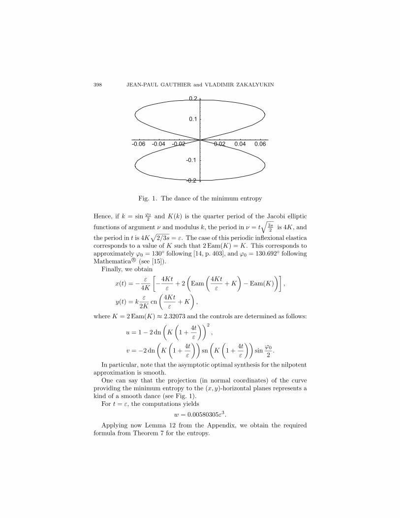
Fig. 1. The dance of the minimum entropy

Hence, if k = sin ϕ02 and K(k) is the quarter period of the Jacobi elliptic

functions of argument ν and modulus k, the period in ν = t√

3s2 is 4K, and

the period in t is 4K√

2/3s = ε. The case of this periodic inflexional elasticacorresponds to a value of K such that 2Eam(K) = K. This corresponds toapproximately ϕ0 = 130◦ following [14, p. 403], and ϕ0 = 130.692◦ followingMathematica r© (see [15]).

Finally, we obtain

x(t) = − ε

4K

[−4Kt

ε+ 2

(Eam

(4Ktε

+K

)− Eam(K)

)],

y(t) = kε

2Kcn

(4Ktε

+K

),

where K = 2Eam(K) ≈ 2.32073 and the controls are determined as follows:

u = 1 − 2 dn(K

(1 +

4tε

))2

,

v = −2 dn(K

(1 +

4tε

))sn

(K

(1 +

4tε

))sin

ϕ0

2.

In particular, note that the asymptotic optimal synthesis for the nilpotentapproximation is smooth.

One can say that the projection (in normal coordinates) of the curveproviding the minimum entropy to the (x, y)-horizontal planes represents akind of a smooth dance (see Fig. 1).

For t = ε, the computations yields

w = 0.00580305ε3.

Applying now Lemma 12 from the Appendix, we obtain the requiredformula from Theorem 7 for the entropy.


9. Appendix

9.1. Appendix 1. Estimating an entropy of a motion planning problemΣ = (Γ,Δ, g), we consider the following problem.

Problem (Qω) (ω is small). Find l∗ = inf{length(γ); γ is admissible,ω-interpolating, dom(γ) = [0, tγ ], γ(0) = Γ(0), γ(tγ) = Γ(1)}.

Problem (Qω) has a subproblem (Pw0ω ).

Problem (Pw0ω ) (ω is small). Given Γ(w0), find w∗ = sup{w; ∃γ admis-

sible, ∃a ≤ ω, γ(0) = Γ(w0), γ(a) = Γ(w0 + w)}.We state (and sketch the proof of) certain basic properties of these prob-

lems.

Lemma 9. In problem (Qω), the minimum l∗ is attained at a ω-interpolating curve γ∗, which is a (finitely) piecewise minimizing geodesic(minimizing pieces have length ≤ω).

Note that the proof of Lemma 9 contains the proof of the following knownresult.

Lemma 10. In problem (Pw0ω ), the maximum is attained at a curve

which is a minimizing geodesic, and a = ω.

Sketch of the proof of Lemma 9. In these purely local constructions (aroundΓ), we can assume that the orthonormal frame F = (F1, . . . , Fn−p) has com-pact support. Thus, we can assume that the trajectories under considerationare defined up to t = +∞. Let un be a minimizing sequence of controls,and let xn be the corresponding sequence of trajectories. Reparametriz-ing by a constant factor dt = αdτ the trajectory which was initially ar-clength parametrized, we can assume that the domain of un and xn is [0, 1]and un are uniformly bounded in L∞[0, 1] and in L2[0, 1]. Also, denotingthe L2-norm by ‖ · ‖, we obtain that the sequence ‖un‖ = length(xn) isbounded. Thus, we see that un weakly converges in L2 to some weak limitu∗, and the corresponding limit trajectory is x∗. The input-output mappingu(·) → x(·) is a continuous mapping from the space (L2[0, 1], weak) to thespace (C0[0, 1], uniform). Moreover,

length(x∗) ≤ ‖u∗‖ ≤ lim ‖un‖ = l∗.

Therefore, (u∗, x∗) is a minimizing trajectory and x∗(0) = Γ(0) andx∗(1) = Γ(1).

Let us show that x∗ is ω-interpolating; assume the contrary. ThenLemma 11 implies that x∗ contains a piece-segment P of the length l exceed-ing ω, with the corresponding control Q (defined on the same interval) suchthat P does not intersect Γ. Denote by (Pn, Qn) the segments of the trajec-tories and controls (xn, un) restricted to the same domain of the length l.


The uniform convergence of xn implies that for sufficiently large n, Pn doesnot intersect Γ. Also,

lim length(Pn) =√l lim ‖Qn‖ ≥

√l‖Q‖ ≥ length(P ) > ω.

Therefore, (un, xn) is not ω-interpolating, a contradiction.If an interpolating piece of x∗ is not a minimizing geodesic, then it is

easy to see that x∗ is not optimal.

Lemma 11. If γ(0), γ(1) ∈ Γ and each segment of γ of the length >ωcontains a point of Γ, then Γ is ω-interpolating.

This is obvious, as well as the fact (which we use extensively through-out the paper) that γ is ω-interpolated with a finite number of pieces oflength ≤ω.

Now, given a motion planning problems Σ (in the normal form, withrespect to certain normal coordinates), assume that for all sufficiently smallω, the solutions w∗

ω of Problems (Pwω ) from Lemma 10 satisfy the inequality

Aωp ≤ |w∗ω − w| ≤ Bωp (9.1)

for p = 2 or p = 3.Assume that Γ : [0,W ] → R

n (keeping in mind certain reparametriza-tions, we do not restrict ourselves to the case W = 1).

Lemma 12. Under these assumptions,

W

Bωp≤ E(ω) ≤ W

Aωp+ k, k > 0.

Proof. First, solving repeatedly problems (Pwω ) (for which the extremum is

attained) we construct an ω-interpolating curve γ∗ such that

length(γ∗) ≤ W

Aωp−1+ kω, k > 0.

The term kω is introduced to compensate the upper-boundary effect. Thiscan easily be done using Lemma 4.

Then, by definition,

E(ω) ≤ length(γ∗)ω

≤ W

Aωp+ k.

Second, let γω be any ω-interpolating curve, arclength parametrized. Lett0 = 0 < t1 < · · · < tn = tγω

be the interpolation points. We have, byassumption (applying (9.1) for ω = ti+1 − ti), the following estimates:

|wi+1 − wi| ≤ B|ti+1 − ti|p,|wi+1 − wi|

ωp≤ B(

|ti+1 − ti|ω

)p ≤ B|ti+1 − ti|

ω,


since |ti+1 − ti| ≤ ω. This implies

|ti+1 − ti| ≥ |wi+1 − wi|Bωp−1

≥ wi+1 − wi

Bωp−1,

and since l(γω) =∑ |ti+1 − ti|, we obtain

l(γω) ≥ W

Bωp−1.

Hencel(γω)ω

≥ W

Bωp,

which consequently implies that taking the infimum over all ω-interpolatingcurves γω, the required estimate holds:

E(ω) ≥ W

Bωp.

The lemma is proved.

9.2. Appendix 2. Below, ‖ · ‖ means the L2-norm.Let M , Lj , j = 1, . . . , p−1, be linearly independent skew-symmetric ma-

trices (note that this independence is due to the one-step bracket-generatingassumption). We use the abbreviated notation N(λ) = M + λN for

M +p−1∑j=1

λjLj . let λ∗ be such that

α = ‖N(λ∗)‖ = infλ

‖N(λ)‖.Such λ∗ automatically exists by the assumption of the independence, and‖N(λ∗)‖ > 0.

Assume that ‖N(λ)‖ is a smooth function in λ at least in a neighbor-hood V0 of λ∗. This holds, in particular, when the maximum moduluseigenvalue

√−1α (=√−1‖N(λ∗)‖) of N(λ∗) is simple. (In fact, in this

case, α(λ) = ‖N(λ)‖ is an analytic function in λ on V0).Under these assumptions, the following crucial property, used throughout

the paper, holds (we recall its proof from [8]).

Lemma 13. The set

B ={

(x′My, x′L1y, . . . , x′Lp−1y); ‖x‖, ‖y‖ ≤ 1

}⊂ R

p

is strictly convex in the direction (1, 0, . . . , 0).

Proof. Without loss of generality, we can assume that λ∗ = 0. Then on V0

we have

α(λ) = sup‖x‖=‖y‖=1

x′N(λ)y = sup‖x‖,‖y‖≤1

x′N(λ)y = X(λ)′N(λ)Y (λ),

‖X(λ)‖ = ‖Y (λ)‖ = 1.


Obviously, we can find smooth in λ vectors X(λ) and Y (λ) satisfying theserelations.

Hence we can write

X(λ) = X + λX +O2(λ),

Y (λ) = Y + λY +O2(λ),

α(λ) = α+ λα+O2(λ).

Then the equality 1 = 〈X(λ),X(λ)〉 implies

1 = 〈X,X〉 + 2λ〈X, X〉 +O2(λ).

This and a similar equation for Y imply

〈X, X〉 = 0, 〈Y, Y 〉 = 0. (9.2)

We also have

α(λ) = X(λ)′N(λ)Y (λ) ≥ α ∀λ ∈ V0

and

α+ λα+O2(λ) =(X + λX +O2(λ)

)′(M + λL)(Y + λY +O2(λ)

)

= X ′MY + λ(X ′MY +X ′MY +X ′LY

)+O2(λ)

= α+ λ(X ′MY +X ′MY +X ′LY

)+O2(λ) ≥ α, ∀α ∈ V0.

This implies that X ′MY + X ′MY + X ′LY = 0. Since, by definition,MX = −αY and MY = αX, we have X ′MY = αX ′X = 0 by (9.2). SinceX ′MY = −Y ′MX = αY ′Y = 0, we obtain X ′LY = 0.

This means that

(X ′MY,X ′L1Y, . . . ,X′Lp−1Y ) = (‖N(λ∗)‖, 0, . . . , 0) ∈ B,

infλ

sup(w,z)∈B

(w + λz) = ‖N(λ∗)‖ = (1, λ∗1, . . . , λ∗p−1) ·

⎛

⎜⎜⎜⎜⎝

‖N(λ∗)‖0. . .. . .0

⎞

⎟⎟⎟⎟⎠,

which is exactly condition (P2) from Definition 1. Hence, B is strictlyconvex in the direction (1, 0, . . . , 0).

Corollary 1 (in the notation of Sec. 2). If Bt is not strictly convex inthe direction of Γt mod ΔΓ(t), then Mt+ λ∗Lt has a nonsimple maximummodulus eigenvalue.

Recall another fact (see [8, Lemma 9, item 3]) used throughout the paper.


Lemma 14. For a generic one-step bracket-generating Σ, except for fi-nite subset of Γ, there exists a smooth mapping w → λ∗(w) such that∥∥∥∥∥M(w) +

p−1∑j=1

λ∗j (w)Lj(w)

∥∥∥∥∥ is the minimum of ‖N(λ)‖.

The proof uses a standard transversality argument.This lemma implies an important fact that, for nilpotent approximation

(4.4), we can (excluding a finite subset of Γ without any influence on theestimates of the entropy and complexity) make the change of variables:

w = w +p−1∑j=1

λ∗j (w)yj . This is a change of the parametrization of S, which

preserves the parametrization of Γ and yields normal coordinates (x, y, w),provided that (x, y, w) are normal. In these new coordinates,

‖M(w)‖ = infλ

∥∥∥∥∥∥M(w) +

p−1∑

j=1

λjLj(w)

∥∥∥∥∥∥.

References

1. A. A. Agrachev, H. E. A. Chakir, and J. P. Gauthier, Sub-Riemannianmetrics on R

3. In: Geometric Control and Nonholonomic Mechanics,Mexico City (1996), pp. 29–76. Proc. Can. Math. Soc. 25 (1998).

2. A. A. Agrachev and J. P. Gauthier, Sub-Riemannian metrics andisoperimetric problems in the contact case. J. Math. Sci. 103 (2001),No. 6, 639–663.

3. G. Charlot, Quasicontact SR metrics: normal form in R2n, wave front

and caustic in R4. Acta Appl. Math. 74 (2002), No. 3, 217–263.

4. H. E. A. Chakir, J. P. Gauthier, and I. A. K. Kupka, Small sub-Riemannian balls on R

3. J. Dynam. Control Systems 2 (1996), No. 3,359–421.

5. F. H. Clarke, Optimization and nonsmooth analysis. John Wiley & Sons(1983).

6. J. P. Gauthier, F. Monroy-Perez, and C. Romero-Melendez, On com-plexity and motion planning for corank one SR metrics. ESAIM ControlOptim. Calc. Var. 10 (2004), 634–655.

7. J. P. Gauthier and V. Zakalyukin, On the codimension one motionplanning problem. J. Dynam. Control Systems 11 (2005), No. 1, 73–89.

8. , On the one-step bracket-generating motion planning problem.J. Dynam. Control Systems 11 (2005), No. 2, 215–235.

9. , Robot motion planning, a wild case. To appear in Proc 2004Suszdal Conf. on Dynam. Systems (2006).

10. M. Gromov, Carnot–Caratheodory spaces seen from within. Prog. Math.144 (1996), 79–323.


11. F. Jean, Complexity of nonholonomic motion planning. Int. J. Control74 (2001), No. 8, 776–782.

12. , Entropy and complexity of a path in SR geometry. ESAIMControl Optim. Calc. Var. 9 (2003), 485–506.

13. F. Jean and E. Falbel, Measures and transverse paths in SR geometry.J. Anal. Math. 91 (2003), 231–246.

14. A. E. H. Love, A treatise on the mathematical theory of elasticity.Dover, New York (1944).

15. Mathematica r©, Reference manual. France (1997).16. L. Pontryagin, V. Boltyanski, R. Gamkelidze, and E. Michenko, The

mathematical theory of optimal processes. Wiley, New York (1962).

(Received May 30 2005)

Authors’ addresses:Jean-Paul GauthierLE2I, UMR CNRS 5158, Universite de Bourgogne,Bat. Mirande, BP 47870, 21078, Dijon CEDEX FranceE-mail: [email protected]

Vladimir ZakalyukinMoscow State University, 119993, Leninski Gori, 1, Moscow, RussiaE-mail: [email protected]

ON THE MOTION PLANNING PROBLEM, … · Journal of Dynamical and Control Systems, Vol. 12, No. 3,...

Documents

Transcript of ON THE MOTION PLANNING PROBLEM, … · Journal of Dynamical and Control Systems, Vol. 12, No. 3,...