1 © 2016 Astro Ltd Printed in the UK

Laser Physics Letters

J Dimitrijević et al

On the efficiency of 1D atom localisation via EIT in a degenerate two-level atomic system

Printed in the UK

045202

LPLABC

© 2016 Astro Ltd

2016

13

Laser Phys. Lett.

LPL

1612-2011

10.1088/1612-2011/13/4/045202

4

Laser Physics Letters

1. Introduction

During the past two decades there has been considerable atten-tion in developing various techniques for precision position measurements of an atom moving through a standing-wave field [1]. Due to the fact that the dynamics of the atomic sys-tems is position dependent within a standing-wave, by mea-suring the position-dependent quantities of the system, one can attain information on the position of the atom in the sub-wavelength domain. Interest in studying the atom localisation effect lies in potential applications for the precise measure-ment of atom position in laser cooling and trapping of atoms [2, 3], Bose–Einstein condensation [4, 5], atom nanolithogra-phy [6–8], the measurement of the centre-of-mass wave func-tion of moving atoms [9, 10] etc.

Early developed methods for atom localisation were based on measurements of the phase shifts of standing waves [11, 12], or atomic dipole [13, 14], resonance imaging methods [15, 16] entanglement between the atom position and its internal state [17], Ramsey interferometry [18] etc. Recent techniques to achieve atom localisation are mainly based on the atomic coherence of internal states and quantum-interference effects.

Considerable interest is in realising atom localisation by coher-ent population trapping [19] and electromagnetically induced transparency (EIT) [20], also phase-dependent EIT in closed-loop atomic schemes, Autler–Townes microscopy [21], STIRAP (stimulated Raman adiabatic passage) [22] etc. Studies were per-formed by utilising position-dependent quantities like probe field absorption [23, 24], atom excited state population [25–27], spon-taneously emitted photon [21, 28–31] and Raman gain [32, 33].

While early studies on atom localisation were mainly for one-dimensional localisation, recent studies also analyse real-isations of two-dimensional localisation [24, 30, 31], since they provide more information on the atom position, better spatial resolution and could potentially find more applica-tions. Moreover, recent studies [34, 35] suggest the realisation of three-dimensional atom localisation. The newly established domain of subwavelength localisation, named sub-half-wave-length localisation, analyses techniques that give informa-tion on the atom position within the half wavelength distance [29, 36, 37]. Only a few experimental realisations of the atom localisation effect have been performed [34, 38–40] so far.

In studies of atom localisation, an atom is considered to be localised if narrow structures can be observed in the

On the efficiency of 1D atom localisation via EIT in a degenerate two-level atomic system

Jelena Dimitrijević, Dušan Arsenović and Branislav M Jelenković

Institute of Physics, University of Belgrade, Pregrevica 118 11080 Belgrade

E-mail: jelenad@ipb.ac.rs

Received 4 September 2015, revised 26 November 2015Accepted for publication 26 January 2016Published 4 March 2016

AbstractWe analyse one-dimensional (1D) subwavelength atom localisation in a cold atomic medium under the action of two optical fields, the standing-wave and travelling probe fields, in the presence of a magnetic field. Optical Bloch equations are solved numerically for the hyperfine atomic transition →= =F F2 1g e of the 87Rb D1 line. All Zeeman sublevels are included in the calculations. This atomic scheme allows electromagnetically induced transparency (EIT) if the applied magnetic field is zero or small. The results for the position-dependent probe absorption are presented for two configurations, depending on the orientation of the magnetic field with respect to the optical fields’ polarisations. The efficiency of the atom localisation is analysed for a large range of field intensities and applied magnetic fields. The observed behaviour of the probe absorption is analysed through the effects of EIT induced by two fields of various strengths and its dependence on the applied magnetic fields.

Keywords: 1D atom localisation, electromagnetically induced transparency, Zeeman effect

(Some figures may appear in colour only in the online journal)Letter

Astro Ltd

JW

1612-2011/16/045202+8$33.00

doi:10.1088/1612-2011/13/4/045202Laser Phys. Lett. 13 (2016) 045202 (8pp)

J Dimitrijević et al

2

localisation pattern, i.e. a position dependence of measur-able quantity. The number of narrow structures in one sub-wavelength domain shows the detecting probability, the width shows the localisation precision, while the positions indicate where the atom is localised. Most theoretical studies on atom localisation use simple atomic schemes constituted of sev-eral atomic levels. This enables analytical expressions to be obtained from which one can read the choice of parameters (field strengths, detunings, relative phase etc) which yields the most efficient atom localisation.

We perform a numerical study and analyse the efficiency of one-dimensional (1D) atom localisation by using two orthogonal optical fields, the standing-wave and travelling probe fields. Atom localisation studies often use the detuning of the optical field from the resonance for control of localisa-tion. Here, we assume that both fields are on the resonance of

→= =F F2 1g e transition, D1 line in 87Rb, while the shift of energy levels from the resonances is done by applying a magn-etic field. This atomic scheme is known to support Zeeman EIT, a quantum phenomenon due to the coherent superposi-tion of magnetic sublevels, manifested in the reduced absorp-tion of the optical field if zero or a small magn etic field is applied. The numerical calculations are done by solving Optical Bloch equations  for a multiple-level atomic scheme with all the Zeeman sublevels taken into consideration. Two configurations, with different orientations of magn etic field, along the standing-wave or along the probe field polarisa-tion, are analysed. The advantage of numerical analysis is that we can apply arbitrary strengths of optical and magn-etic fields. The optical fields’ intensities range from 10−4 to 102 mW cm−2, the while magnetic fields range from 0 to  G5 . We analyse the behaviour of the localisation patterns obtained from the probe field absorption, investigating the effects of standing-wave and probe intensities, and also the influence of magnetic fields on the efficiency of 1D atom localisation.

2. 1D atom localisation schemes and theoretical model

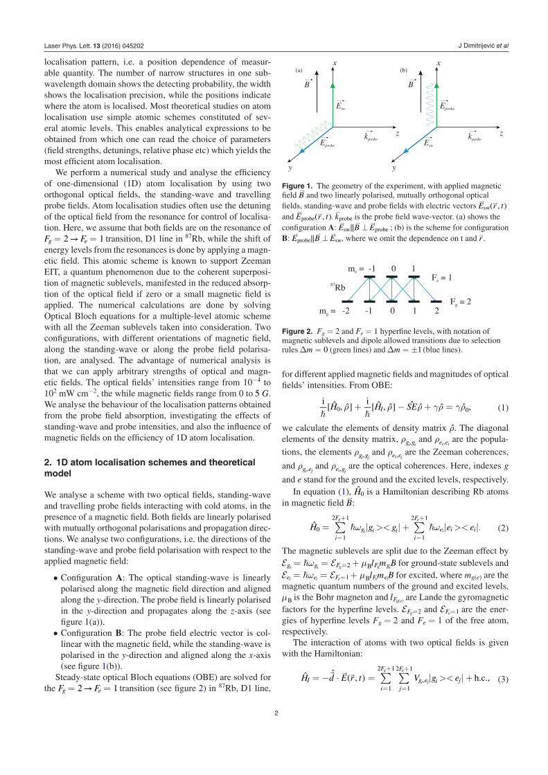
We analyse a scheme with two optical fields, standing-wave and travelling probe fields interacting with cold atoms, in the presence of a magnetic field. Both fields are linearly polarised with mutually orthogonal polarisations and propagation direc-tions. We analyse two configurations, i.e. the directions of the standing-wave and probe field polarisation with respect to the applied magnetic field:

• Configuration A: The optical standing-wave is linearly polarised along the magnetic field direction and aligned along the y-direction. The probe field is linearly polarised in the y-direction and propagates along the z-axis (see figure 1(a)).

• Configuration B: The probe field electric vector is col-linear with the magnetic field, while the standing-wave is polarised in the y-direction and aligned along the x-axis (see figure 1(b)).

Steady-state optical Bloch equations (OBE) are solved for the →= =F F2 1g e transition (see figure 2) in 87Rb, D1 line,

for different applied magnetic fields and magnitudes of optical fields’ intensities. From OBE:

[ ˆ ˆ] [ ˆ ˆ] ˆ ˆ ˆ ˆρ ρ ρ γρ γρ+ − + =� �

H H SEi

,i

, ,I0 0 (1)

we calculate the elements of density matrix ρ. The diagonal elements of the density matrix, ρg g,i i

and ρe e,i i are the popula-

tions, the elements ρg g,i j and ρe e,i j

are the Zeeman coherences,

and ρg e,i j and ρe g,i j

are the optical coherences. Here, indexes g

and e stand for the ground and the excited levels, respectively.In equation (1), H0 is a Hamiltonian describing Rb atoms

in magnetic field →B:

∑ ∑ω ω= | >< | + | >< |=

+

=

+

� �H g g e e .i

F

g i ii

F

e i i01

2 1

1

2 1g

i

e

iˆ (2)

The magnetic sublevels are split due to the Zeeman effect by ω µ= = +=E � E l m Bg g F F g2 Bi i g g i

for ground-state sublevels and ω µ= = +=E � E l m Be e F F e1 Bi i e e i for excited, where mg(e) are the

magnetic quantum numbers of the ground and excited levels, µB is the Bohr magneton and ( )lFg e are Lande the gyromagnetic factors for the hyperfine levels. =EF 2g and =EF 1e are the ener-gies of hyperfine levels Fg = 2 and Fe = 1 of the free atom, respectively.

The interaction of atoms with two optical fields is given with the Hamiltonian:

ˆ ˆ ( )→ → → ∑ ∑= − ⋅ = | >< | +

=

+

=

+

H d E r t V g e, h.c.,Ii

F

j

F

g e i j1

2 1

1

2 1

,

g e

i j (3)

Figure 1. The geometry of the experiment, with applied magnetic field

→B and two linearly polarised, mutually orthogonal optical

fields, standing-wave and probe fields with electric vectors ( )→ →E r t,sw and ( )→ →E r t,probe .

→kprobe is the probe field wave-vector. (a) shows the

configuration A: ∥ ⊥→ → →E B Esw probe ; (b) is the scheme for configuration

B: ∥ ⊥→ → →E B Eprobe sw, where we omit the dependence on t and →r .

)b()a(x

y

z

Esw

Eprobe

kprobe

B

x

y

z

Eprobe

Esw

kprobe

B

Figure 2. Fg = 2 and Fe = 1 hyperfine levels, with notation of magnetic sublevels and dipole allowed transitions due to selection rules ∆ =m 0 (green lines) and ∆ = ±m 1 (blue lines).

m = -1 0 1e

m = -2 -1 0 1 2g

F = 2g

87RbF = 1e

Laser Phys. Lett. 13 (2016) 045202

J Dimitrijević et al

3

where →d is the electric dipole operator and ( )

→ →E r t, is the total electric field oscillating with angular frequency

ω =−= =E E

�lFe Fg1 2, i.e. both fields are on the resonance of

→= =F F2 1g e transition, the D1 line in 87Rb. Vg e,i j are the

matrix elements of the electric dipole interaction. SE stands for the spontaneous emission operator with rate Γ. We assume relaxation of all the density matrix elements with small rate γ Γ� due to the mechanism like the finite time of flight or collisional decay [41]. The term ˆγρ0 describes the repopula-tion of the atomic sample at the same rate, where ρ0 describes atoms in their initial state, equal population of the ground Zeeman sublevels. As we are considering cold atomic sample, the role of Doppler broadening is not discussed.

We apply a Raman–Nath approximation [42], i.e. the centre-of-mass position of an atom along the direction of the standing-wave field is nearly constant and therefore we neglect the atom’s kinetic energy in the Hamiltonian. An electric dipole and rotating-wave approximations were applied. The quantisation axis is taken along magnetic field vector

→B, and

equations (1) are solved in the rotated coordinate system for all Zeeman sublevels of the Fg = 2 and Fe = 1 hyperfine levels.

With the quantisation axis along magnetic field vector, two configurations allow different dipole-allowed transitions between the Zeeman magnetic sublevels in the considered atomic scheme (see figure 2 and the indicated different col-ours). For the first configuration A, the standing-wave field is π-polarised and ∆ =m 0 transitions are allowed, while the lin-early polarised probe field introduces multiple Λ-schemes with σ+ and σ− light components of equal strength. Conversely, for the configuration B, for the probe field the selection rule ∆ =m 0 stands, while for the standing-wave field the selec-tion rules are ∆ = ±m 1.

We calculate the probe absorption coefficient Aprobe as an imaginary part of the complex susceptibility tensor diagonal elements. For the configuration A, with the probe field along the y-axis, the probe absorption is calculated from:

( ) [ (

)]

χε

ρ ρ

ρ ρ ρ ρ

= = +

+ + + +

− − −

−

AeRN

EIm Im

i

6 23 2 3

3 3 3 3 2

cg e g e

g e g e g e g e

probe probe0 probe

, ,

, , , ,

2 1 1 0

0 1 0 1 1 0 2 1

(4)

and for the configuration B and →Eprobe along the x-axis is given

as:

( ) [

( )]

χε

ρ ρ ρ

= =

× + +− −

AeRN

EIm Im

6

3 2 3 3 ,

c

e g e g e g

probe probe0 probe

, , ,1 1 0 0 1 1

(5)

where Nc is the atom concentration, e is the elementary charge, ε0 is the permittivity of the vacuum and ∥ ∥→=< >R J r Jg e is the transition dipole matrix element.

3. Results and discussion

We calculate the localisation patterns, that is, the probe absorp-tion versus the normalised positions (k xsw or k ysw ) within the

standing-wave range { }−λ λ,2 2

. To calculate the localisation

structures we use the same values of parameters for both con-figurations: the concentration of Rb atoms in the sample is

 =N 10c m16 1

3, the relaxation rate is  γ = Γ0.001 and the spon-

taneous emission rate is πΓ = 2 5.750 06 MHz. The results are analysed for the range of applied standing-wave and probe field intensities (Isw and Iprobe, respectively) from 10−4 to 102 mW cm−2. We vary the magnetic field between 0 and  G5 , staying in the vicinity of the EIT resonance.

Besides obtaining narrow structures in the localisation pattern, important for an experimental realisation of atom localisation is the ability to resolve the absorption levels in the localisation pattern. Therefore, we analysed the behaviour of the base-level, contrast and also full width at half maximum (FWHM) of the narrow peaks shown in the localisation pat-terns. In order to determine the structures in the localisation pattern, we calculated extrema of the Aprobe versus k xsw (or k ysw ) curve. The structure is defined by one of these extrema, as its middle point, and its two adjacent extrema. The base-level represents the minimal absorption of the structure and the contrast is taken between the central and border extrema, where we take the smaller value if the peak is asymmetric. The FWHM is calculated as the width of the peak at half of the contrast height.

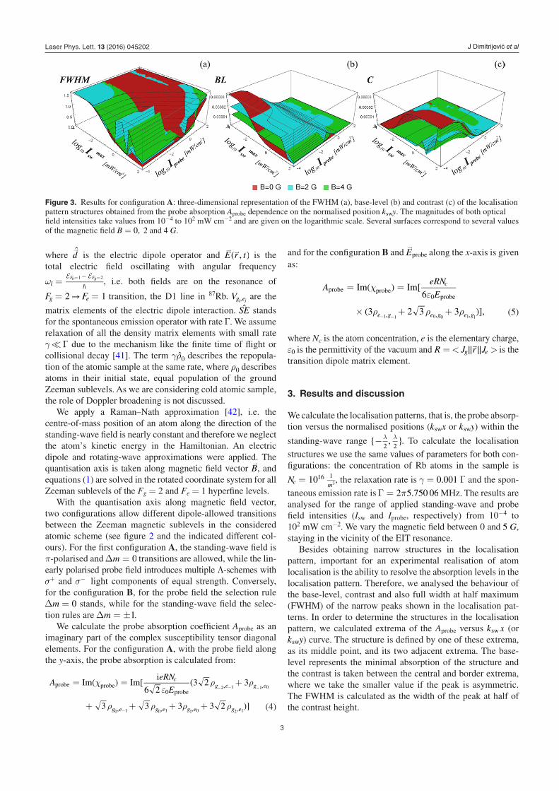
Figure 3. Results for configuration A: three-dimensional representation of the FWHM (a), base-level (b) and contrast (c) of the localisation pattern structures obtained from the probe absorption Aprobe dependence on the normalised position k ysw . The magnitudes of both optical field intensities take values from 10−4 to 102 mW cm−2 and are given on the logarithmic scale. Several surfaces correspond to several values of the magnetic field  =B 0, 2 and  G4 .

Laser Phys. Lett. 13 (2016) 045202

J Dimitrijević et al

4

3.1. Configuration A

In configuration A, as shown in figure  1(a), standing-wave electric vector

→Esw is parallel to the magnetic field

→B. In

figure 3 we present the results for the FWHM (a), base-level (b) and contrast (c) of the localisation pattern structures for intensities, Iprobe and Isw

max, from 10−4 to 102 mW cm−2 given on the logarithmic scale. The results presented here are for three values of the magnetic field,  =B 0, 2 and  G4 , while our analysis includes more values. The results for the widths of the structures show that, for < −I 10sw

max 2 mW cm−2, informa-tion on the atom position is available in a very broad region,

i.e. the localisation structures have FWHM ≈ λ4, which indi-

cates poor localisation precision. With the increase in Iswmax the

widths reduce and for <I 1probe mW cm−2 extremely narrow structures can be obtained. The base level of the structures strongly depends on the probe field intensity and is low for

>I 1probe mW cm−2. The contrast of the localisation structures is higher if Isw

max is large and Iprobe is small. In the following, we present some results from the previously discussed range of intensities, which show efficient localisation and also the effects of the magnetic field on the atom localisation.

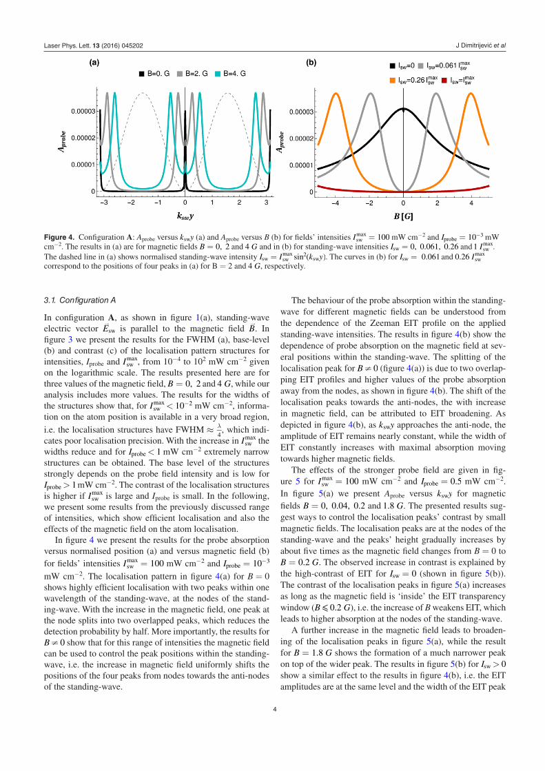
In figure 4 we present the results for the probe absorption versus normalised position (a) and versus magnetic field (b) for fields’ intensities =I 100sw

max mW cm−2 and = −I 10probe3

mW cm−2. The localisation pattern in figure 4(a) for B = 0 shows highly efficient localisation with two peaks within one wavelength of the standing-wave, at the nodes of the stand-ing-wave. With the increase in the magnetic field, one peak at the node splits into two overlapped peaks, which reduces the detection probability by half. More importantly, the results for ≠B 0 show that for this range of intensities the magnetic field

can be used to control the peak positions within the standing-wave, i.e. the increase in magnetic field uniformly shifts the positions of the four peaks from nodes towards the anti-nodes of the standing-wave.

The behaviour of the probe absorption within the standing-wave for different magnetic fields can be understood from the dependence of the Zeeman EIT profile on the applied standing-wave intensities. The results in figure 4(b) show the dependence of probe absorption on the magnetic field at sev-eral positions within the standing-wave. The splitting of the localisation peak for ≠B 0 (figure 4(a)) is due to two overlap-ping EIT profiles and higher values of the probe absorption away from the nodes, as shown in figure 4(b). The shift of the localisation peaks towards the anti-nodes, the with increase in magnetic field, can be attributed to EIT broadening. As depicted in figure 4(b), as k ysw approaches the anti-node, the amplitude of EIT remains nearly constant, while the width of EIT constantly increases with maximal absorption moving towards higher magnetic fields.

The effects of the stronger probe field are given in fig-ure  5 for =I 100sw

max mW cm−2 and =I 0.5probe mW cm−2. In figure  5(a) we present Aprobe versus k ysw for magnetic fields    =B 0, 0.04, 0.2 and  G1.8 . The presented results sug-gest ways to control the localisation peaks’ contrast by small magnetic fields. The localisation peaks are at the nodes of the standing-wave and the peaks’ height gradually increases by about five times as the magnetic field changes from B = 0 to

 =B G0.2 . The observed increase in contrast is explained by the high-contrast of EIT for =I 0sw (shown in figure  5(b)). The contrast of the localisation peaks in figure 5(a) increases as long as the magnetic field is ‘inside’ the EIT transparency window ( ⩽  B G0.2 ), i.e. the increase of B weakens EIT, which leads to higher absorption at the nodes of the standing-wave.

A further increase in the magnetic field leads to broaden-ing of the localisation peaks in figure  5(a), while the result for  =B G1.8 shows the formation of a much narrower peak on top of the wider peak. The results in figure 5(b) for >I 0sw show a similar effect to the results in figure 4(b), i.e. the EIT amplitudes are at the same level and the width of the EIT peak

Figure 4. Configuration A: Aprobe versus k ysw (a) and Aprobe versus B (b) for fields’ intensities =I 100swmax mW cm−2 and = −I 10probe

3 mW cm−2. The results in (a) are for magnetic fields  =B 0, 2 and  G4 and in (b) for standing-wave intensities    =I 0, 0.061, 0.26sw and  I1 sw

max. The dashed line in (a) shows normalised standing-wave intensity ( )=I I k ysinsw sw

max 2sw . The curves in (b) for  =I 0.061sw and  I0.26 sw

max correspond to the positions of four peaks in (a) for B = 2 and  G4 , respectively.

Laser Phys. Lett. 13 (2016) 045202

J Dimitrijević et al

5

increases with the standing-wave intensity. For a small range of standing-wave intensities, the dependence of Aprobe ver-sus B shows overlapping for values of B outside of the EIT

peaks indicating that the standing-wave intensity reached saturation intensity [43], i.e. a further increase in Isw does not lead to higher one-photon absorption. The above explains the

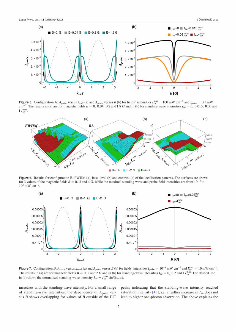
Figure 5. Configuration A: Aprobe versus k ysw (a) and Aprobe versus B (b) for fields’ intensities =I 100swmax mW cm−2 and =I 0.5probe mW

cm−2. The results in (a) are for magnetic fields    =B 0, 0.04, 0.2 and  G1.8 and in (b) for standing-wave intensities    =I 0, 0.015, 0.06sw and  I1 sw

max.

Figure 6. Results for configuration B: FWHM (a), base-level (b) and contrast (c) of the localisation patterns. The surfaces are drawn for 3 values of the magnetic fields  =B 0, 2 and 4 G, while the maximal standing wave and probe field intensities are from 10−4 to 102 mW cm−2.

Figure 7. Configuration B: Aprobe versus k xsw (a) and Aprobe versus B (b) for fields’ intensities = −I 10probe4 mW cm−2 and =I 10sw

max mW cm−2. The results in (a) are for magnetic fields  =B 0, 1 and  G2 and in (b) for standing-wave intensities  =I 0, 0.2sw and  I1 sw

max. The dashed line in (a) shows the normalised standing-wave intensity =I I k xsinsw sw

max 2sw( ).

Laser Phys. Lett. 13 (2016) 045202

J Dimitrijević et al

6

nearly constant probe absorption around the nodes for value  =B G1.8 in figure 5(a) and the formation of another narrow

peak.

3.2. Configuration B

In configuration B, as presented in figure 1(b), the probe field is oriented along the magnetic field and the quantisation axis. Figure 6 shows the results for the FWHMs (a), base-contrast (b) and contrast (c) of the localisation pattern structures. The results for the structure widths show that the precision for atom localisation increases when intensity ⩾ −I 10sw

max 2 mW cm−2. The base-level of the localisation structures is low if either the field intensity is larger than 1 mW cm−2. The results for the contrast suggest that the range <I 1probe mW cm−2 and > −I 10sw

max 2 mW cm−2 induces a higher contrast of locali-sation structures. In short, the results in figure 6 show good localisation with high precision, low base-level and high con-trast for small Iprobe and large Isw

max .

In figure  7(a) we present the localisation patterns for = −I 10probe

4 mW cm−2 and =I 10swmax mW cm−2 and for three

values of the magnetic field  =B 0, 1 and  G2 . The results show excellent atom localisation at the nodes of the standing-wave. At and around the anti-nodes positions’ absorption is completely suppressed due to high standing-wave intensities exceeding the saturation intensity. The wide absorption maxi-mum for =I 0sw in figure  7(b) corresponds to one-photon absorption since π-polarised light cannot induce EIT [41, 44]. The height of ther localisation peaks in figure 7(a) at the nodes decreases slightly with the increase in B due to the shifts of magnetic levels and lower absorption due to detuning from the resonance. The localisation peaks are broadened for small values of Isw or near the nodes, where EIT is weaker for larger B (see figure 7(b)) resulting in a slight reduction in localisa-tion efficiency.

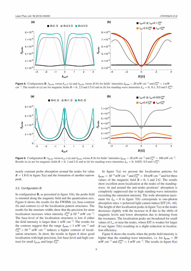
Figure 8 shows the results when the probe field intensity is higher than the standing-wave intensities, i.e. for =I 20probe mW cm−2 and =I 1sw

max mW cm−2. The results in figure 8(a)

Figure 8. Configuration B: Aprobe versus k xsw (a) and Aprobe versus B (b) for fields’ intensities =I 20probe mW cm−2 and =I 1swmax mW

cm−2. The results in (a) are for magnetic fields  =B 0, 2.5 and  G3.5 and in (b) for standing-wave intensities    =I 0, 0.1, 0.5sw and  I1 swmax.

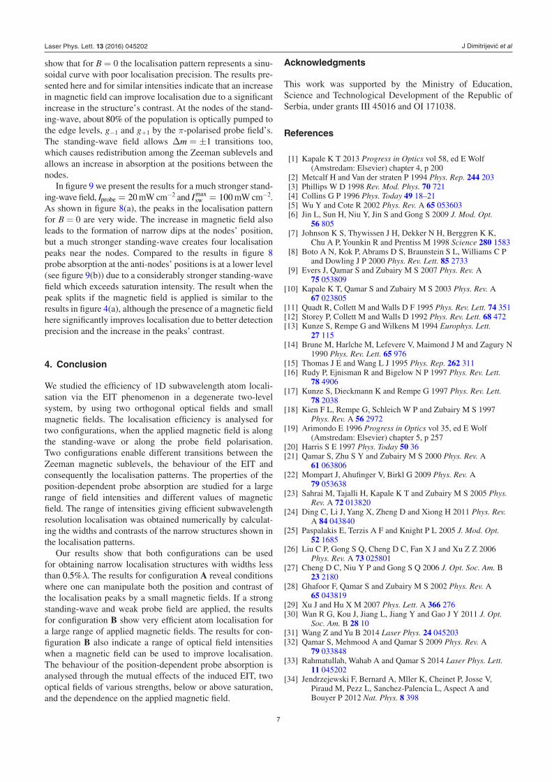
Figure 9. Configuration B: Aprobe versus k xsw (a) and Aprobe versus B (b) for fields’ intensities =I 20probe mW cm−2 and =I 100swmax mW cm−2.

Results in (a) are for magnetic fields  =B 0, 1 and  G3 and in (b) for standing-wave intensities    =I 0, 0.025, 0.5sw and  I1 swmax.

Laser Phys. Lett. 13 (2016) 045202

J Dimitrijević et al

7

show that for B = 0 the localisation pattern represents a sinu-soidal curve with poor localisation precision. The results pre-sented here and for similar intensities indicate that an increase in magnetic field can improve localisation due to a significant increase in the structure’s contrast. At the nodes of the stand-ing-wave, about 80% of the population is optically pumped to the edge levels, g−1 and g+1 by the π-polarised probe field’s. The standing-wave field allows ∆ = ±m 1 transitions too, which causes redistribution among the Zeeman sublevels and allows an increase in absorption at the positions between the nodes.

In figure 9 we present the results for a much stronger stand-ing-wave field, =I 20probe mW cm−2 and =I 100sw

max mW cm−2. As shown in figure 8(a), the peaks in the localisation pattern for B = 0 are very wide. The increase in magnetic field also leads to the formation of narrow dips at the nodes’ position, but a much stronger standing-wave creates four localisation peaks near the nodes. Compared to the results in figure  8 probe absorption at the anti-nodes’ positions is at a lower level (see figure 9(b)) due to a considerably stronger standing-wave field which exceeds saturation intensity. The result when the peak splits if the magnetic field is applied is similar to the results in figure 4(a), although the presence of a magnetic field here significantly improves localisation due to better detection precision and the increase in the peaks’ contrast.

4. Conclusion

We studied the efficiency of 1D subwavelength atom locali-sation via the EIT phenomenon in a degenerate two-level system, by using two orthogonal optical fields and small magn etic fields. The localisation efficiency is analysed for two configurations, when the applied magnetic field is along the standing-wave or along the probe field polarisation. Two configurations enable different transitions between the Zeeman magnetic sublevels, the behaviour of the EIT and consequently the localisation patterns. The properties of the position-dependent probe absorption are studied for a large range of field intensities and different values of magnetic field. The range of intensities giving efficient subwavelength resolution localisation was obtained numerically by calculat-ing the widths and contrasts of the narrow structures shown in the localisation patterns.

Our results show that both configurations can be used for obtaining narrow localisation structures with widths less than λ0.5% . The results for configuration A reveal conditions where one can manipulate both the position and contrast of the localisation peaks by a small magnetic fields. If a strong standing-wave and weak probe field are applied, the results for configuration B show very efficient atom localisation for a large range of applied magnetic fields. The results for con-figuration B also indicate a range of optical field intensities when a magnetic field can be used to improve localisation. The behaviour of the position-dependent probe absorption is analysed through the mutual effects of the induced EIT, two optical fields of various strengths, below or above saturation, and the dependence on the applied magnetic field.

Acknowledgments

This work was supported by the Ministry of Education, Science and Technological Development of the Republic of Serbia, under grants III 45016 and OI 171038.

References

[1] Kapale K T 2013 Progress in Optics vol 58, ed E Wolf (Amstredam: Elsevier) chapter 4, p 200

[2] Metcalf H and Van der straten P 1994 Phys. Rep. 244 203 [3] Phillips W D 1998 Rev. Mod. Phys. 70 721 [4] Collins G P 1996 Phys. Today 49 18–21 [5] Wu Y and Cote R 2002 Phys. Rev. A 65 053603 [6] Jin L, Sun H, Niu Y, Jin S and Gong S 2009 J. Mod. Opt.

56 805 [7] Johnson K S, Thywissen J H, Dekker N H, Berggren K K,

Chu A P, Younkin R and Prentiss M 1998 Science 280 1583 [8] Boto A N, Kok P, Abrams D S, Braunstein S L, Williams C P

and Dowling J P 2000 Phys. Rev. Lett. 85 2733 [9] Evers J, Qamar S and Zubairy M S 2007 Phys. Rev. A

75 053809 [10] Kapale K T, Qamar S and Zubairy M S 2003 Phys. Rev. A

67 023805 [11] Quadt R, Collett M and Walls D F 1995 Phys. Rev. Lett. 74 351 [12] Storey P, Collett M and Walls D 1992 Phys. Rev. Lett. 68 472 [13] Kunze S, Rempe G and Wilkens M 1994 Europhys. Lett.

27 115 [14] Brune M, Harlche M, Lefevere V, Maimond J M and Zagury N

1990 Phys. Rev. Lett. 65 976 [15] Thomas J E and Wang L J 1995 Phys. Rep. 262 311 [16] Rudy P, Ejnisman R and Bigelow N P 1997 Phys. Rev. Lett.

78 4906 [17] Kunze S, Dieckmann K and Rempe G 1997 Phys. Rev. Lett.

78 2038 [18] Kien F L, Rempe G, Schleich W P and Zubairy M S 1997

Phys. Rev. A 56 2972 [19] Arimondo E 1996 Progress in Optics vol 35, ed E Wolf

(Amstredam: Elsevier) chapter 5, p 257 [20] Harris S E 1997 Phys. Today 50 36 [21] Qamar S, Zhu S Y and Zubairy M S 2000 Phys. Rev. A

61 063806 [22] Mompart J, Ahufinger V, Birkl G 2009 Phys. Rev. A

79 053638 [23] Sahrai M, Tajalli H, Kapale K T and Zubairy M S 2005 Phys.

Rev. A 72 013820 [24] Ding C, Li J, Yang X, Zheng D and Xiong H 2011 Phys. Rev.

A 84 043840 [25] Paspalakis E, Terzis A F and Knight P L 2005 J. Mod. Opt.

52 1685 [26] Liu C P, Gong S Q, Cheng D C, Fan X J and Xu Z Z 2006

Phys. Rev. A 73 025801 [27] Cheng D C, Niu Y P and Gong S Q 2006 J. Opt. Soc. Am. B

23 2180 [28] Ghafoor F, Qamar S and Zubairy M S 2002 Phys. Rev. A

65 043819 [29] Xu J and Hu X M 2007 Phys. Lett. A 366 276 [30] Wan R G, Kou J, Jiang L, Jiang Y and Gao J Y 2011 J. Opt.

Soc. Am. B 28 10 [31] Wang Z and Yu B 2014 Laser Phys. 24 045203 [32] Qamar S, Mehmood A and Qamar S 2009 Phys. Rev. A

79 033848 [33] Rahmatullah, Wahab A and Qamar S 2014 Laser Phys. Lett.

11 045202 [34] Jendrzejewski F, Bernard A, Mller K, Cheinet P, Josse V,

Piraud M, Pezz L, Sanchez-Palencia L, Aspect A and Bouyer P 2012 Nat. Phys. 8 398

Laser Phys. Lett. 13 (2016) 045202

J Dimitrijević et al

8

[35] Qi Y, Zhou F, Huang T, Niu Y and Gong S 2012 J. Mod Opt. 59 1092

[36] Shen W B, Hu X M and Xu J 2008 J. Phys. B: At. Mol. Opt. Phys. 41 185502

[37] Shui T, Wang Z, Cao Z and Yu B 2014 Laser Phys. 24 055202

[38] Li H, Sautenkov V A, Kash M M, Sokolov A V, Welch G R, Rostovtsev Y V, Zubairy M S and Scully M O 2008 Phys. Rev. A 78 013803

[39] Proite N A, Simmons Z J and Yavuz D D 2011 Phys. Rev. A 83 041803

[40] Miles J A, Simmons Z J and Yavuz D D 2013 Phys. Rev. X 3 031014

[41] Margalit L, Rosenbluh M and Wilson-Gordon A D 2013 Phys. Rev. A 87 033808

[42] Meystre P and Sargent M III 1999 Elements of Quantum Optics 3rd edn (Berlin: Springer)

[43] Steck D A 2015 Rubidium 87 D Line Data, available online at http://steck.us/alkalidata (revision 2.1.5, 13 January 2015)

[44] Dimitrijević J, Krmpot A, Mijailović M, Arsenović D, Panić B, Grujić Z and Jelenković B M 2008 Phys. Rev. A 77 013814

Laser Phys. Lett. 13 (2016) 045202