Ωnyx User Guide

Ωnyx User Guide

Timo von Oertzen, Andreas M. Brandmaier, and Siny Tsang

Version 1.0-872; July, 1st, 2014

Contents

1 Introduction 2

2 Installing Ωnyx 4

3 Creating Models 63.1 Model Panels . . . . . . . . . . . . . . . . . . . . . . . . . . . . . 63.2 Variables . . . . . . . . . . . . . . . . . . . . . . . . . . . . . . . . 73.3 Paths . . . . . . . . . . . . . . . . . . . . . . . . . . . . . . . . . . 93.4 Editing models . . . . . . . . . . . . . . . . . . . . . . . . . . . . 113.5 Displaying Scripts, Import, and Export . . . . . . . . . . . . . 123.6 Definition Variables . . . . . . . . . . . . . . . . . . . . . . . . . 133.7 Multi Group Models . . . . . . . . . . . . . . . . . . . . . . . . . 133.8 Simulation . . . . . . . . . . . . . . . . . . . . . . . . . . . . . . . 13

4 Estimation of Model Parameters 164.1 Data Panels . . . . . . . . . . . . . . . . . . . . . . . . . . . . . . 164.2 Estimation . . . . . . . . . . . . . . . . . . . . . . . . . . . . . . . 194.3 Mean Structure . . . . . . . . . . . . . . . . . . . . . . . . . . . . 214.4 Model Comparison . . . . . . . . . . . . . . . . . . . . . . . . . . 224.5 Definition Variables . . . . . . . . . . . . . . . . . . . . . . . . . 23

5 Customization 245.1 Layout . . . . . . . . . . . . . . . . . . . . . . . . . . . . . . . . . 245.2 Formatting . . . . . . . . . . . . . . . . . . . . . . . . . . . . . . 255.3 Mathematical symbols . . . . . . . . . . . . . . . . . . . . . . . . 27

A Keyboard Shortcuts 30

1

Chapter 1

Introduction

Ωnyx is a free graphical Structural Equation Modeling (SEM) software forcreating and estimating SEMs. It provides a graphical user interface that fa-cilitates an intuitive creation of models, and a powerful backend for perform-ing maximum likelihood estimation of parameters in models. You can useΩnyx as a stand-alone software or from the statistical computing language R.Ωnyx allows you to import models from OpenMx, a free SEM package for R,and exports scripts to OpenMx, Mplus, lavaan, and sem. Also, publication-quality figures can be exported as vector representation, LATEXcode, or inbitmap representations.

Structural Equation Modeling is a frequently used multivariate analysistechnique in the behavioral and social sciences. SEM are linear models ofboth observed and latent variables and their relationships. The maximum-likelihood-framework allows estimation of structural parameters even on thelatent level by modeling the covariances and expectations of the observedvariables.

There are various text books that cover the essentials of SEM, for exam-ple, Bollen(1989). SEM can be conceived of as a unification of several mul-tivariate analysis techniques under a single framework. Particularly, linearregression, ANOVA, correlation, path analysis, factor analysis, autoregres-sion, and growth curve modeling can be considered special cases of SEM.

Ωnyx is intended to be a teaching tool for SEM. It facilitates a graphicalapproach to modeling that offers an interface to OpenMx, lavaan, sem andMplus code. That is, SE modeling can be taught in a graphical approachwithout the need to teach a specific modeling language. In the progress of acourse, a transition from the purely graphical approach to a specific modelinglanguage can be made. An interactive code view allows users to track andcompare changes to the model specification in the selected scripting languagethat are elicited by changes to the graphical representation.

2

CHAPTER 1. INTRODUCTION 3

The backend of Ωnyx allows to estimate parameters with Maximum Like-lihood or Least Squares. The possible space of solutions is systematicallysearched with multiple start values, which allows to find and weight differentpossible solution, or different local minima of similar fit value. This docu-ment provides a brief introduction to the features of Ωnyx . The creationof models and the basic mechanisms of the underlying estimation engineare explained. More details regarding Ωnyx can be found on the websitehttp://onyx.brandmaier.de.

Chapter 2

Installing Ωnyx

System Requirements

• Operating Systems

– Microsoft Windows 2000/XP/Vista/7/8

– Mac OS X 10.5 or later

– Linux (tested on Ubuntu)

• Java Runtime Environment (JRE; version 1.6 or later)

Install Java

If your system does not have Java, or has an older version of JRE (priorto version 1.6), download Java JRE here: http://java.com/en/download/index.jsp. To check your current JRE version, type (in the terminal): java-version

Java for earlier versions of Mac OS (10.5 or earlier) is supported by Apple;run the Apple updates on your computer to update to the latest version ofjava. Next, go to Applications | Java Preferences; move java SE 6 tothe top.

Run Ωnyx

Download the newest version of Ωnyx from our website: http://onyx.

brandmaier.de.

4

CHAPTER 2. INSTALLING ΩNYX 5

The download will be delivered as a .jar file. Move this file into thedirectory of your choice, or you can leave it on your desktop. Double clickthe onyx file with the suffix .jar to run Ωnyx .

Quick Start

This tutorial covers basic modeling steps in Ωnyx . We recommend exploringfurther features in Ωnyx by right-clicking1 on objects. On a right-click onany object, a context menu containing a list of all operations that can beperformed on the respective object, are listed. This includes right-clicks onthe desktop, which allows to create a new empty model or load data andmodels. Ωnyx also comes with an interactive tutorial which you can startfrom the help menu on the right side of the menu bar.

1All uses of the right mouse button can alternatively be done with the left mouse buttonwhile holding the CTRL key

Chapter 3

Creating Models

3.1 Model Panels

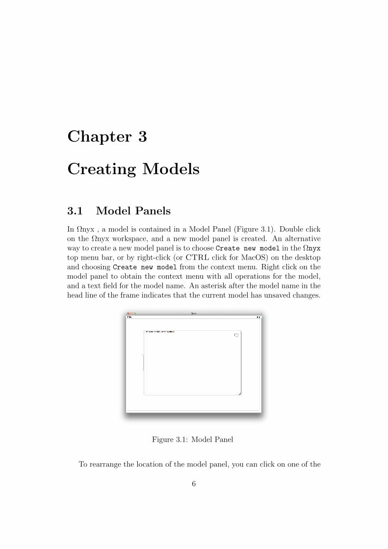
In Ωnyx , a model is contained in a Model Panel (Figure 3.1). Double clickon the Ωnyx workspace, and a new model panel is created. An alternativeway to create a new model panel is to choose Create new model in the Ωnyxtop menu bar, or by right-click (or CTRL click for MacOS) on the desktopand choosing Create new model from the context menu. Right click on themodel panel to obtain the context menu with all operations for the model,and a text field for the model name. An asterisk after the model name in thehead line of the frame indicates that the current model has unsaved changes.

Figure 3.1: Model Panel

To rearrange the location of the model panel, you can click on one of the

6

CHAPTER 3. CREATING MODELS 7

border, and drag the model panel around. To resize the model panel, leftclick and drag the anchor on the bottom right corner.

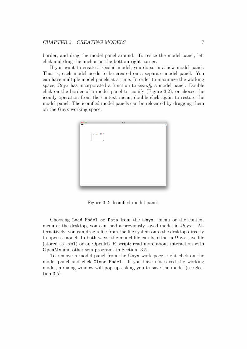
If you want to create a second model, you do so in a new model panel.That is, each model needs to be created on a separate model panel. Youcan have multiple model panels at a time. In order to maximize the workingspace, Ωnyx has incorporated a function to iconify a model panel. Doubleclick on the border of a model panel to iconify (Figure 3.2), or choose theiconify operation from the context menu; double click again to restore themodel panel. The iconified model panels can be relocated by dragging themon the Ωnyx working space.

Figure 3.2: Iconified model panel

Choosing Load Model or Data from the Ωnyx menu or the contextmenu of the desktop, you can load a previously saved model in Ωnyx . Al-ternatively, you can drag a file from the file system onto the desktop directlyto open a model. In both ways, the model file can be either a Ωnyx save file(stored as .xml) or an OpenMx R script; read more about interaction withOpenMx and other sem programs in Section 3.5.

To remove a model panel from the Ωnyx workspace, right click on themodel panel and click Close Model. If you have not saved the workingmodel, a dialog window will pop up asking you to save the model (see Sec-tion 3.5).


3.2 Variables

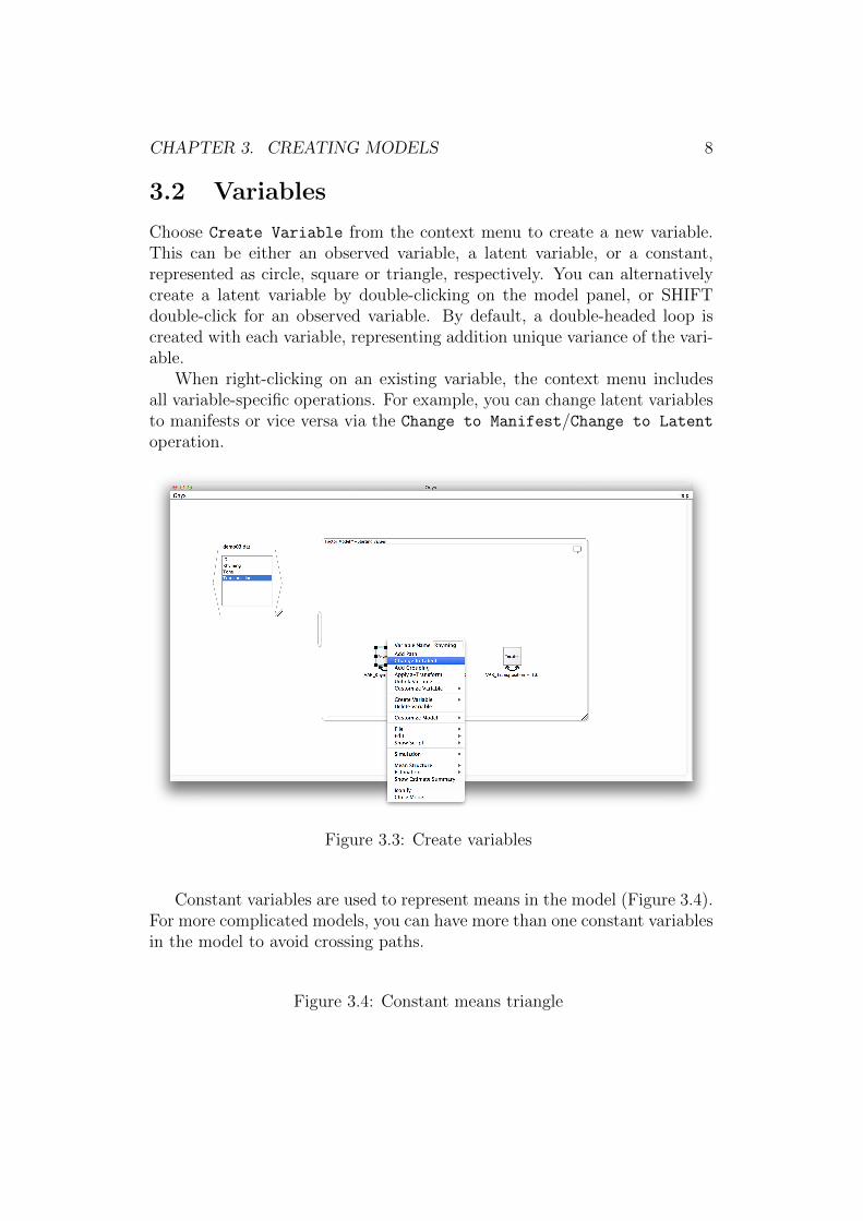
Choose Create Variable from the context menu to create a new variable.This can be either an observed variable, a latent variable, or a constant,represented as circle, square or triangle, respectively. You can alternativelycreate a latent variable by double-clicking on the model panel, or SHIFTdouble-click for an observed variable. By default, a double-headed loop iscreated with each variable, representing addition unique variance of the vari-able.

When right-clicking on an existing variable, the context menu includesall variable-specific operations. For example, you can change latent variablesto manifests or vice versa via the Change to Manifest/Change to Latent

operation.

Figure 3.3: Create variables

Constant variables are used to represent means in the model (Figure 3.4).For more complicated models, you can have more than one constant variablesin the model to avoid crossing paths.

Figure 3.4: Constant means triangle


The appearance of a variable can be changed by choosing Customize

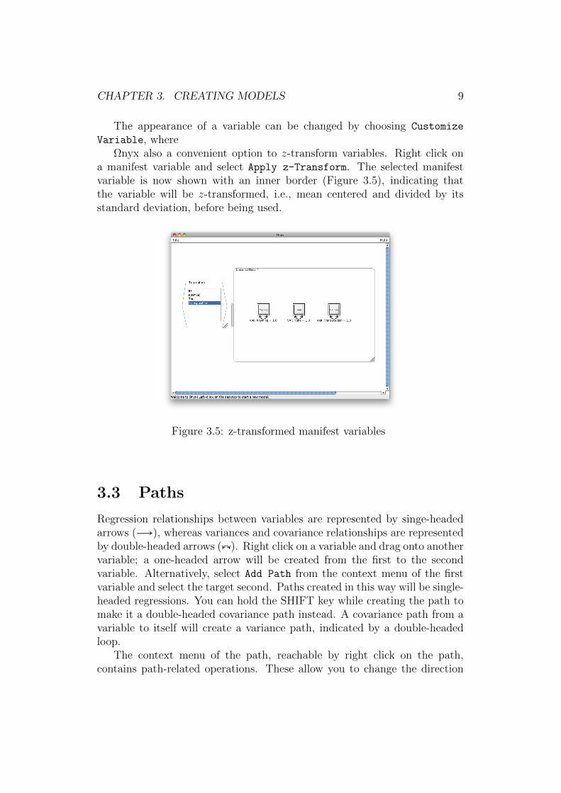
Variable, whereΩnyx also a convenient option to z-transform variables. Right click on

a manifest variable and select Apply z-Transform. The selected manifestvariable is now shown with an inner border (Figure 3.5), indicating thatthe variable will be z-transformed, i.e., mean centered and divided by itsstandard deviation, before being used.

Figure 3.5: z-transformed manifest variables

3.3 Paths

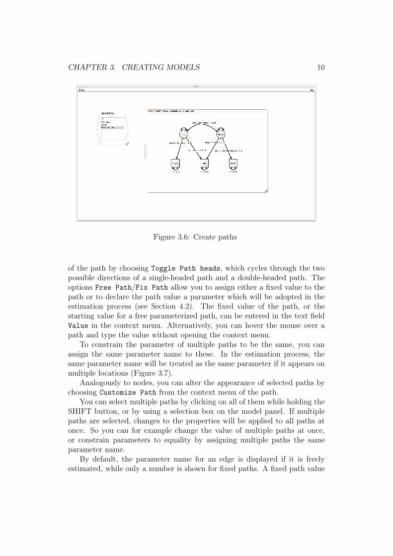
Regression relationships between variables are represented by singe-headedarrows (Ð→), whereas variances and covariance relationships are representedby double-headed arrows (È). Right click on a variable and drag onto anothervariable; a one-headed arrow will be created from the first to the secondvariable. Alternatively, select Add Path from the context menu of the firstvariable and select the target second. Paths created in this way will be single-headed regressions. You can hold the SHIFT key while creating the path tomake it a double-headed covariance path instead. A covariance path from avariable to itself will create a variance path, indicated by a double-headedloop.

The context menu of the path, reachable by right click on the path,contains path-related operations. These allow you to change the direction


Figure 3.6: Create paths

of the path by choosing Toggle Path heads, which cycles through the twopossible directions of a single-headed path and a double-headed path. Theoptions Free Path/Fix Path allow you to assign either a fixed value to thepath or to declare the path value a parameter which will be adopted in theestimation process (see Section 4.2). The fixed value of the path, or thestarting value for a free parameterized path, can be entered in the text fieldValue in the context menu. Alternatively, you can hover the mouse over apath and type the value without opening the context menu.

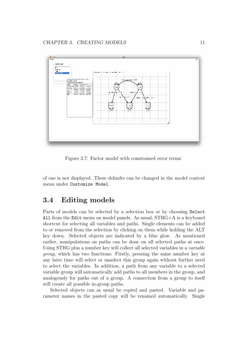
To constrain the parameter of multiple paths to be the same, you canassign the same parameter name to these. In the estimation process, thesame parameter name will be treated as the same parameter if it appears onmultiple locations (Figure 3.7).

Analogously to nodes, you can alter the appearance of selected paths bychoosing Customize Path from the context menu of the path.

You can select multiple paths by clicking on all of them while holding theSHIFT button, or by using a selection box on the model panel. If multiplepaths are selected, changes to the properties will be applied to all paths atonce. So you can for example change the value of multiple paths at once,or constrain parameters to equality by assigning multiple paths the sameparameter name.

By default, the parameter name for an edge is displayed if it is freelyestimated, while only a number is shown for fixed paths. A fixed path value


Figure 3.7: Factor model with constrained error terms

of one is not displayed. These defaults can be changed in the model contextmenu under Customize Model.

3.4 Editing models

Parts of models can be selected by a selection box or by choosing Select

All from the Edit menu on model panels. As usual, STRG+A is a keyboardshortcut for selecting all variables and paths. Single elements can be addedto or removed from the selection by clicking on them while holding the ALTkey down. Selected objects are indicated by a blue glow. As mentionedearlier, manipulations on paths can be done on all selected paths at once.Using STRG plus a number key will collect all selected variables in a variablegroup, which has two functions: Firstly, pressing the same number key atany later time will select or unselect this group again without further needto select the variables. In addition, a path from any variable to a selectedvariable group will automatically add paths to all members in the group, andanalogously for paths out of a group. A connection from a group to itselfwill create all possible in-group paths.

Selected objects can as usual be copied and pasted. Variable and pa-rameter names in the pasted copy will be renamed automatically. Single


actions can be undone or redone. All these options are available in the Edit

menu, or via the standard keyboard shortcuts STRG+C and STRG+V orSHIFT+INSERT and STRG+INSERT for copy and paste, and STRG+Xand STRG+Y for undo and redo.

Two create a new model panel with an exact copy of the whole model, theClone operation in the Edit menu on the model panel can be used. This isparticularly helpful to create a restricted version of a model for a likelihoodratio test (see Section 4.4).

3.5 Displaying Scripts, Import, and Export

The path diagram representation used to create models in Ωnyx can be dis-played as scripts for multiple other sem programs, including OpenMx (bothmatrix and ram notation), lavaan, sem, and Mplus, or in other formal SEMrepresentations, in particular RAM matrices and LISREL matrices. To ac-cess these scripts, choose Show Script in the model’s context panel. Anexternal panel will open that provides a script of the model. You may switchbetween different scripts with the context menu of the script panel. Anychanges in the model (e.g., deletion of edges or addition of new nodes) willinstantaneously be reflected in the script. Keeping both the graphical andthe textual representation next to each other opens a simple way to accessthe scripting languages for the above mentioned programs, in particular forstudents in classroom settings.

Using the File menu in the model panel, the model can be exportedinto a script file directly, which can then be used in other programs. Alsorefer to Section 4.2 to see how Ωnyx can run the scripts directly and use theestimates in the path diagram.

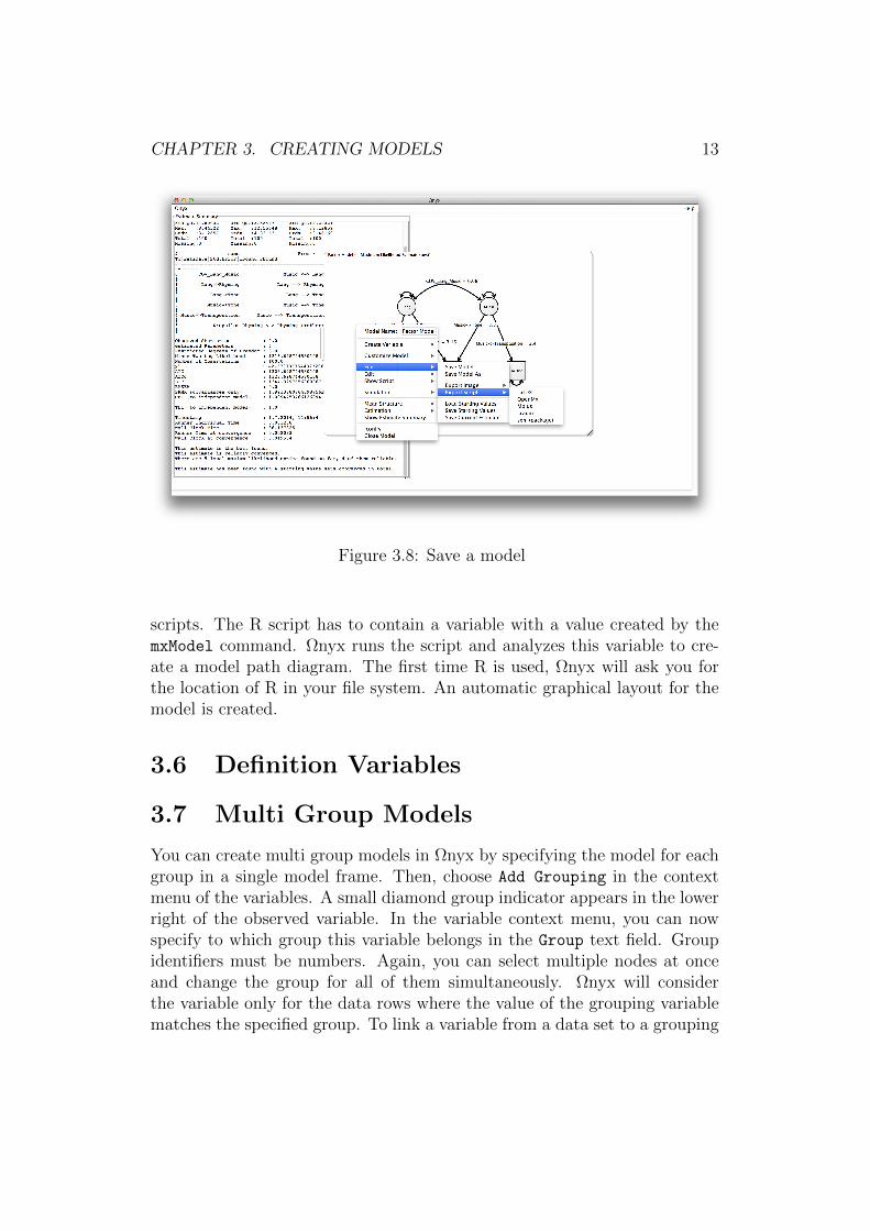
The File menu also allows to save the model in the Ωnyx native format,which is an XML format describing the model path diagram (Figure 3.8).This file can at any time be loaded again by dragging the file onto the desktopor by the Load Model or Data menu on the desktop.

For publications, the path diagram of the model can be exported in var-ious graphical formats using the Export Image operation in the File menuof the model panel. These formats include vector graphics or pixel basedgraphic formats. Alternatively, you can select some or all parts of a model,copy these parts, and paste them in an external graphic program or a slidepresentation program, as for example Microsoft Power Point; a graphical rep-resentation of the path diagram will directly be exported into those programsfor further editing or for presentations.

In addition to the native format, Ωnyx allows to import data from OpenMx


Figure 3.8: Save a model

scripts. The R script has to contain a variable with a value created by themxModel command. Ωnyx runs the script and analyzes this variable to cre-ate a model path diagram. The first time R is used, Ωnyx will ask you forthe location of R in your file system. An automatic graphical layout for themodel is created.

3.6 Definition Variables

3.7 Multi Group Models

You can create multi group models in Ωnyx by specifying the model for eachgroup in a single model frame. Then, choose Add Grouping in the contextmenu of the variables. A small diamond group indicator appears in the lowerright of the observed variable. In the variable context menu, you can nowspecify to which group this variable belongs in the Group text field. Groupidentifiers must be numbers. Again, you can select multiple nodes at onceand change the group for all of them simultaneously. Ωnyx will considerthe variable only for the data rows where the value of the grouping variablematches the specified group. To link a variable from a data set to a grouping


indicator, see Section 4.1.

3.8 Simulation

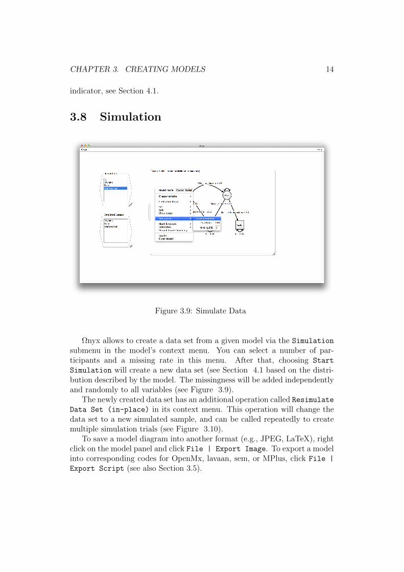
Figure 3.9: Simulate Data

Ωnyx allows to create a data set from a given model via the Simulation

submenu in the model’s context menu. You can select a number of par-ticipants and a missing rate in this menu. After that, choosing Start

Simulation will create a new data set (see Section 4.1 based on the distri-bution described by the model. The missingness will be added independentlyand randomly to all variables (see Figure 3.9).

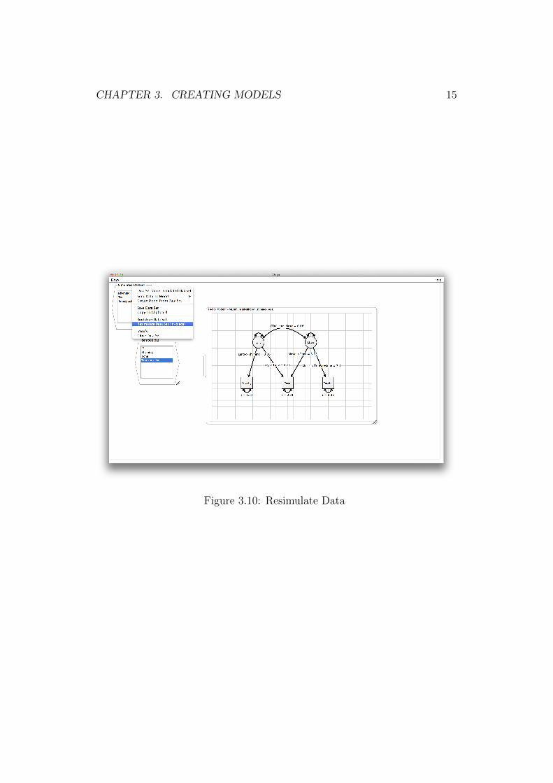
The newly created data set has an additional operation called Resimulate

Data Set (in-place) in its context menu. This operation will change thedata set to a new simulated sample, and can be called repeatedly to createmultiple simulation trials (see Figure 3.10).

To save a model diagram into another format (e.g., JPEG, LaTeX), rightclick on the model panel and click File | Export Image. To export a modelinto corresponding codes for OpenMx, lavaan, sem, or MPlus, click File |

Export Script (see also Section 3.5).


Figure 3.10: Resimulate Data

Chapter 4

Estimation of ModelParameters

4.1 Data Panels

Before Ωnyx can start the estimation process, the model needs to be con-nected to a data set. To load an existing data set, click Load Model or Data

in the Ωnyx top menu bar. You can also right click on the workspace andchoose Load Model or Data from the context menu. If you do not have anexisting data set, you can choose Load tutorial data on the Ωnyx topmenu bar to load a tutorial data set. In the following examples, the tuto-rial data set User Guide Factor Example was used. Alternatively, you canagain drag a data file from the file system on the desktop and drop it there.You can also copy a data set in a different program (e.g., Microsoft Excelor a text editor) and choose Paste in the context menu of the desktop todirectly paste an array of numbers as a data set into Ωnyx . Data files canbe tab-separated (*.dat), comma-separated (*.csv), or SPSS (*.sav) files.

Ωnyx allows raw data files and covariance (or distribution) data files. Forraw data files, the units of observations (e.g., participants) each have one row,while the columns reflect the variables. The first row can, but does not haveto, contain the variable names. Missing values in the data set can be denotedby empty cells, NA, MISS, or -999. Covariance data sets have to contain thekeyword COVARIANCE, followed by an array of K×K numbers for K variablescontaining the covariance matrix of the observed data. The covariance canbe written fully or in lower left triangular format. The covariance data setmay additionally specify means with the keyword MEAN followed by a singlerow of K mean values. If no means are given, means are assumed to bezero. The keyword SAMPLE SIZE followed by a single integer number can be

16

CHAPTER 4. ESTIMATION OF MODEL PARAMETERS 17

used to specify the number of participants. By default, this value is one ina covariance data set. Finally, the keyword OBSERVED VARIABLES followedby K tab-separated character strings can be used to specify the names ofthe variables. Only the keyword COVARIANCE is required. The keywords canappear in any order.

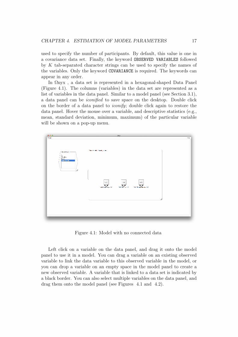
In Ωnyx , a data set is represented in a hexagonal-shaped Data Panel(Figure 4.1). The columns (variables) in the data set are represented as alist of variables in the data panel. Similar to a model panel (see Section 3.1),a data panel can be iconified to save space on the desktop. Double clickon the border of a data panel to iconify ; double click again to restore thedata panel. Hover the mouse over a variable, and descriptive statistics (e.g.,mean, standard deviation, minimum, maximum) of the particular variablewill be shown on a pop-up menu.

Figure 4.1: Model with no connected data

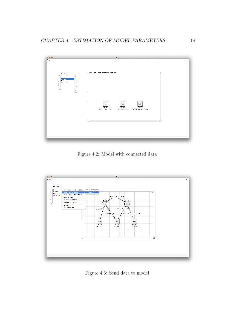
Left click on a variable on the data panel, and drag it onto the modelpanel to use it in a model. You can drag a variable on an existing observedvariable to link the data variable to this observed variable in the model, oryou can drop a variable on an empty space in the model panel to create anew observed variable. A variable that is linked to a data set is indicated bya black border. You can also select multiple variables on the data panel, anddrag them onto the model panel (see Figures 4.1 and 4.2).


Figure 4.2: Model with connected data

Figure 4.3: Send data to model


Note that you can create models without having a Data Panel; Ωnyx offersseveral options to connect models with data sets. Using the context menu ofthe data set, you can choose Create Model from Data Set to create a newdata set which starts with an observed variables for reach variable in the dataset. You can also choose Send Data to Model and select on existing modelto link all variables in the data set to the model by matching the variablenames (see Figure 4.3).

Ωnyx does not provide a in-build editor for data sets, but you can selectCopy to Clipboard on a data set to copy the content of the data file intoanother program, as for example Microsoft Excel or another spreadsheetsoftware. You can edit the data there and copy and paste the data set backinto Ωnyx . You can also choose save to save the data set as a tab separatedfile.

The context menu also allows you to draw a single bootstrap sample froman existing data set by choosing Bootstrap Data from the context menu.This will create a new data set consisting of N draws with replacement fromthe source data set. The context menu in the new data set has an optionRebootstrap Data Set (in-place) that allows to draw new samples atany time.

4.2 Estimation

Once all observed variables in a model are linked to a data set, Ωnyx imme-diately starts a maximum likelihood estimation that finds the best values forall free parameters to make the model distribution be as close to the datadistribution as possible. A tool symbol in the model panel will indicate theprocess. As soon as a converged result is available, the parameter valuesfor all free parameter will show the estimated result; for small models, thishappens mostly instantaneous.

Changes to the model are reflected by simultaneous changes (if any) tothe parameter shown in the model. So all changes are directly reflected in thevisual representation. To view the estimation result in a table, double-click onthe results handle on the left of the model panel to open the Results Drawer.It gives a quick overview over all estimated parameters, there standard error,and the z-transformed parameter estimates. You can double-click the resultsdrawer to close it again.

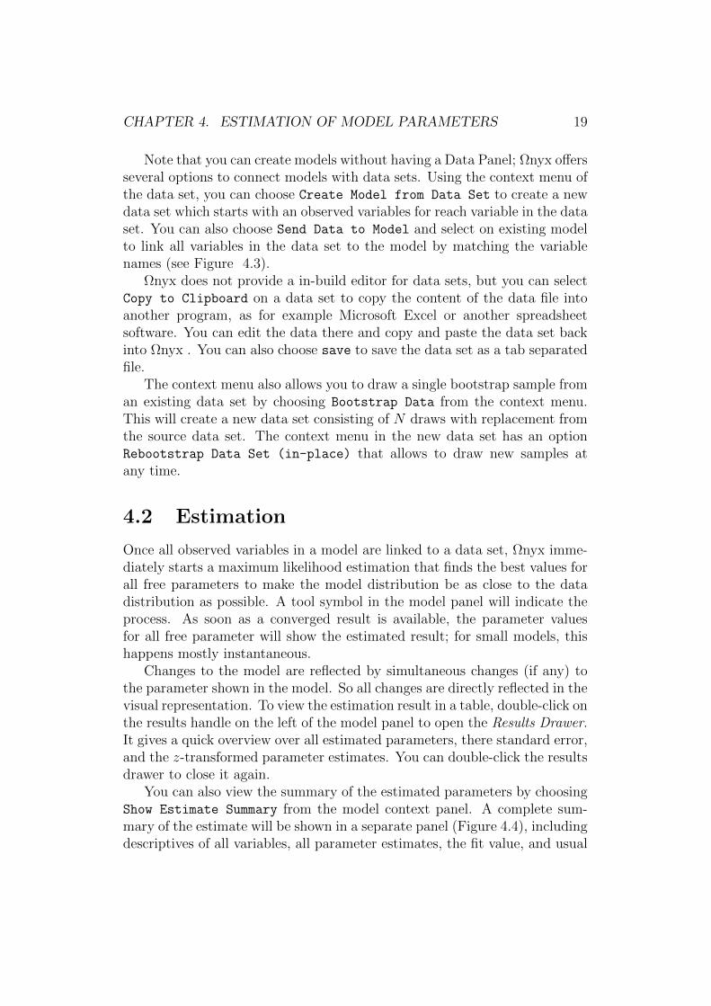
You can also view the summary of the estimated parameters by choosingShow Estimate Summary from the model context panel. A complete sum-mary of the estimate will be shown in a separate panel (Figure 4.4), includingdescriptives of all variables, all parameter estimates, the fit value, and usual


fit indices. You can copy this text, or save it as a text file using the save

operation from the context menu.

Figure 4.4: Model with estimate summary

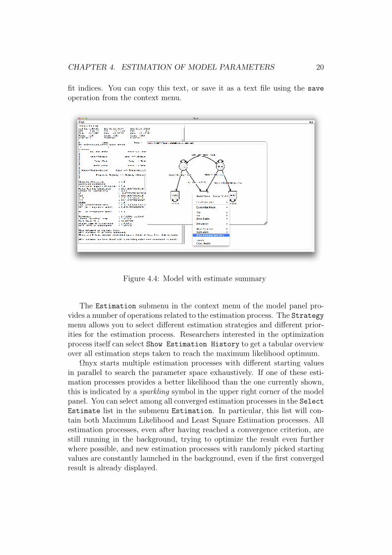
The Estimation submenu in the context menu of the model panel pro-vides a number of operations related to the estimation process. The Strategymenu allows you to select different estimation strategies and different prior-ities for the estimation process. Researchers interested in the optimizationprocess itself can select Show Estimation History to get a tabular overviewover all estimation steps taken to reach the maximum likelihood optimum.

Ωnyx starts multiple estimation processes with different starting valuesin parallel to search the parameter space exhaustively. If one of these esti-mation processes provides a better likelihood than the one currently shown,this is indicated by a sparkling symbol in the upper right corner of the modelpanel. You can select among all converged estimation processes in the SelectEstimate list in the submenu Estimation. In particular, this list will con-tain both Maximum Likelihood and Least Square Estimation processes. Allestimation processes, even after having reached a convergence criterion, arestill running in the background, trying to optimize the result even furtherwhere possible, and new estimation processes with randomly picked startingvalues are constantly launched in the background, even if the first convergedresult is already displayed.


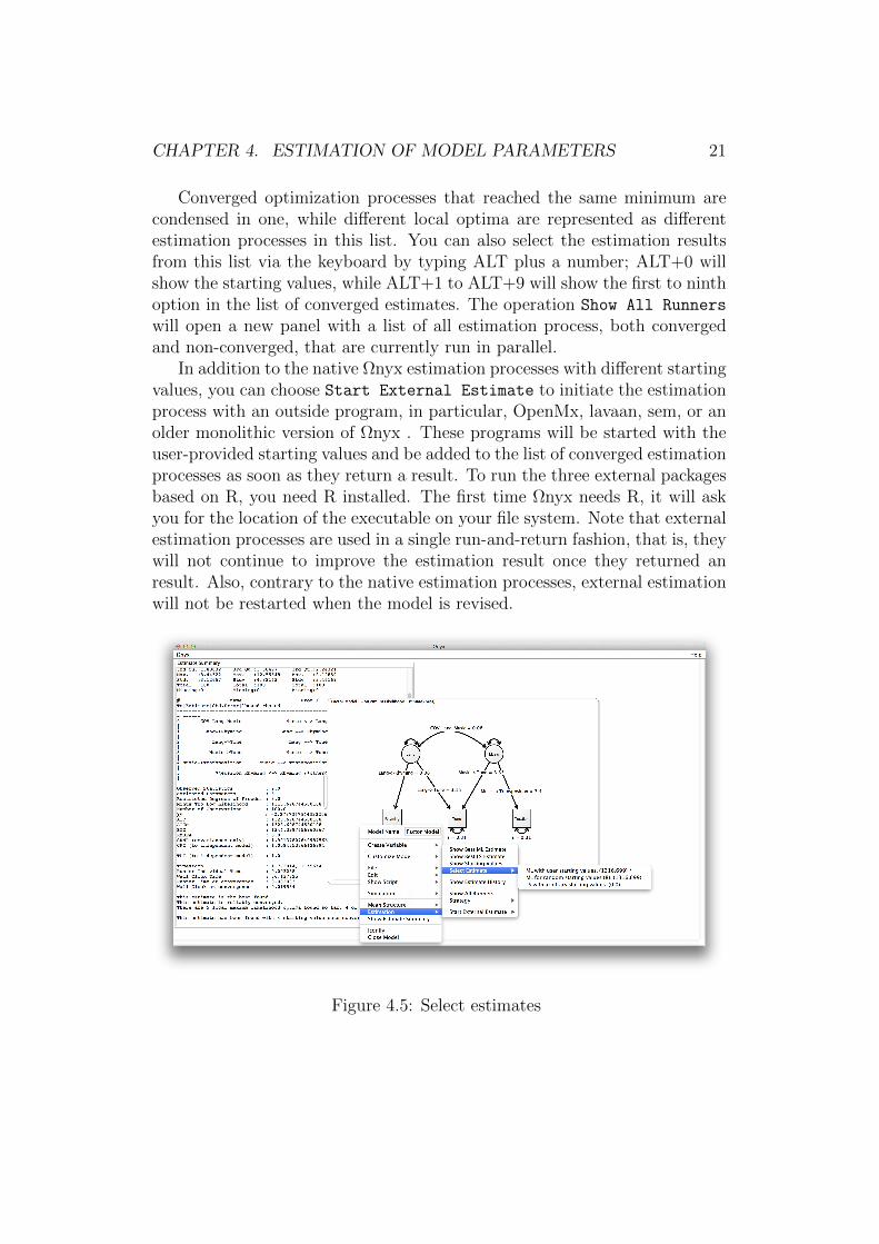
Converged optimization processes that reached the same minimum arecondensed in one, while different local optima are represented as differentestimation processes in this list. You can also select the estimation resultsfrom this list via the keyboard by typing ALT plus a number; ALT+0 willshow the starting values, while ALT+1 to ALT+9 will show the first to ninthoption in the list of converged estimates. The operation Show All Runners

will open a new panel with a list of all estimation process, both convergedand non-converged, that are currently run in parallel.

In addition to the native Ωnyx estimation processes with different startingvalues, you can choose Start External Estimate to initiate the estimationprocess with an outside program, in particular, OpenMx, lavaan, sem, or anolder monolithic version of Ωnyx . These programs will be started with theuser-provided starting values and be added to the list of converged estimationprocesses as soon as they return a result. To run the three external packagesbased on R, you need R installed. The first time Ωnyx needs R, it will askyou for the location of the executable on your file system. Note that externalestimation processes are used in a single run-and-return fashion, that is, theywill not continue to improve the estimation result once they returned anresult. Also, contrary to the native estimation processes, external estimationwill not be restarted when the model is revised.

Figure 4.5: Select estimates


4.3 Mean Structure

Ωnyx provides two options for the treatment of data means. You can choosethe desired treatment from the Mean Structure list in the context menu ofthe model panel. Explicit Means will assume that your model contains allmeans explicitly, using constant variables. Observed variables that are notconnected, directly or indirectly, to a constant variable are assumed to havea fixed mean of zero. This option is advised if your model considers bothfixed and random effects.

The Saturated Mean structure indicates that all variables will be mean-centered before fitting, which for full data sets coincides with estimating themean of every observed variable freely. This option is advised if your modelis about the covariances of the data, and non-zero means, if any, are not tobe considered for the estimation process.

By default, Ωnyx will automatically choose the more appropriate whennecessary. In particular, when you start adding variables to an empty model,a saturated model is assumed. As soon as a constant variable is added to themodel, Ωnyx will switch to an explicit mean structure. If, on the other hand,variables are connected to the model that have non-zero mean even thoughno constant variables are used in the model, Ωnyx will assume saturatedmeans. A warning symbol in the upper right corner indicates when thischange occurred.

4.4 Model Comparison

Two nested models can be compared in Ωnyx using the Likelihood Ratio(LR) test. A model is considered to be nested in another model if restrictionsare imposed on one or more parameters of the second model. The LR testcompares and tests the difference in log likelihood of the two models.

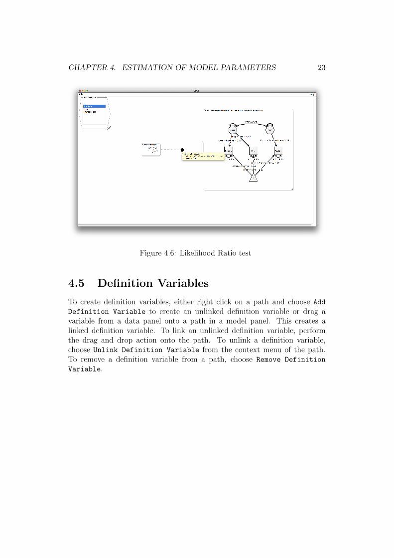
To conduct a LR test, create two nested models. For example, you couldcreate a model, clone it using the Edit submenu, and fix one or more param-eters to zero in the clone. Connect the same data sets to both models. Now,right-click on one model and drag it to the other model, as if creating a pathfrom one to the other model. A dashed line connecting the two model panelsappears indicating a LR comparison (Figure 4.6). Hover the mouse over theblack dot in the middle of the dashed line, and the results from the LR testwill be shown on a pop-up menu. You can also conduct multiple LR testssimultaneously by connecting multiple models. The LR connection betweenmodels can also be drawn when the model are iconified, which increases theoverview of the user.


Figure 4.6: Likelihood Ratio test

4.5 Definition Variables

To create definition variables, either right click on a path and choose Add

Definition Variable to create an unlinked definition variable or drag avariable from a data panel onto a path in a model panel. This creates alinked definition variable. To link an unlinked definition variable, performthe drag and drop action onto the path. To unlink a definition variable,choose Unlink Definition Variable from the context menu of the path.To remove a definition variable from a path, choose Remove Definition

Variable.

Chapter 5

Customization

5.1 Layout

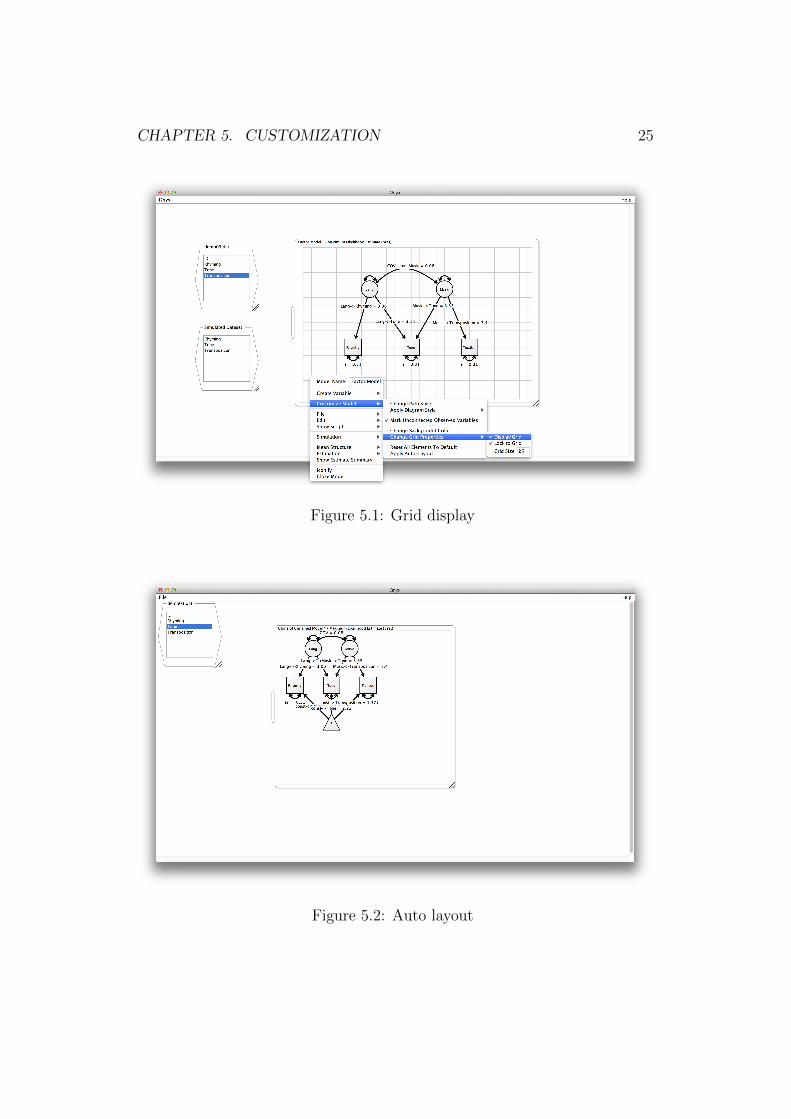
Grid A grid supports you in laying out the components of a graph. Rightclick on the model panel, click Customize Model | Change Grid Properties

| Display Grid to show grid; click Display Grid again to hide grid (Figure5.1(. Click Lock To Grid to enable snapping new variables to grid. You canalso use the keyboard shortcut CTRL/CMD + G. In the same menu, the textfield Grid Size allows you to change the width between grid lines.

Auto layout Right click on the model panel, click Customize Model |

Apply Auto Layout to allow automatic layout of the model. The Auto lay-out function aligns the variables and maximizes the space on the model panel(Figure 5.2).

Reset The visual reset function resets all variable and path properties todefault settings. Right click on the model panel, click Customize Model |

Reset All Elements To Default. Variables are aligned to the grid andvariables are resized into the same size.

5.2 Formatting

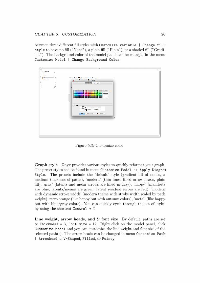
Color To customize the color of variables, right click on the selected vari-able, click Customize variable | Change Line/Fill Color. Color can beselected from a color-wheel window (Figure 5.3(. Similarly, you can customizethe color of paths. Right click on a path, click Change Path Color. If mul-tiple variables/paths are selected (shift + left click), you can customizethe color of the selected variable/path group. Furthermore, you can choose

24

CHAPTER 5. CUSTOMIZATION 25

Figure 5.1: Grid display

Figure 5.2: Auto layout


between three different fill styles with Customize variable | Change fill

style to have no fill (”None”), a plain fill (”Plain”), or a shaded fill (”Gradi-ent”). The background color of the model panel can be changed in the menuCustomize Model | Change Background Color.

Figure 5.3: Customize color

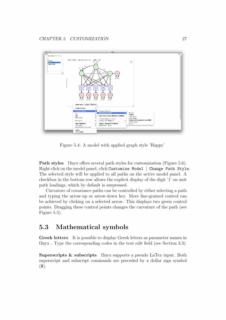
Graph style Ωnyx provides various styles to quickly reformat your graph.The preset styles can be found in menu Customize Model -> Apply Diagram

Style. The presets include the ’default’ style (gradient fill of nodes, amedium thickness of paths), ’modern’ (thin lines, filled arrow heads, plainfill), ’gray’ (latents and mean arrows are filled in gray), ’happy’ (manifestsare blue, latents/means are green, latent residual errors are red), ’modernwith dynamic stroke width’ (modern theme with stroke width scaled by pathweight), retro orange (like happy but with autumn colors), ’metal’ (like happybut with blue/gray colors). You can quickly cycle through the set of stylesby using the shortcut Control + L.

Line weight, arrow heads, and & font size By default, paths are setto Thickness = 3, Font size = 12. Right click on the model panel, clickCustomize Model and you can customize the line weight and font size of theselected path(s). The arrow heads can be changed in menu Customize Path

| Arrowhead as V-Shaped, Filled, or Pointy.


Figure 5.4: A model with applied graph style ’Happy’

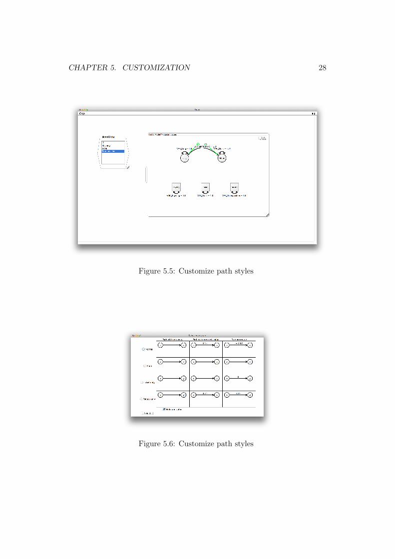
Path styles Ωnyx offers several path styles for customization (Figure 5.6).Right click on the model panel, click Customize Model ∣ Change Path Style.The selected style will be applied to all paths on the active model panel. Acheckbox in the bottom row allows the explicit display of the digit ’1’ on unitpath loadings, which by default is surpressed.

Curvature of covariance paths can be controlled by either selecting a pathand typing the arrow-up or arrow-down key. More fine-grained control canbe achieved by clicking on a selected arrow. This displays two green controlpoints. Dragging these control points changes the curvature of the path (seeFigure 5.5).

5.3 Mathematical symbols

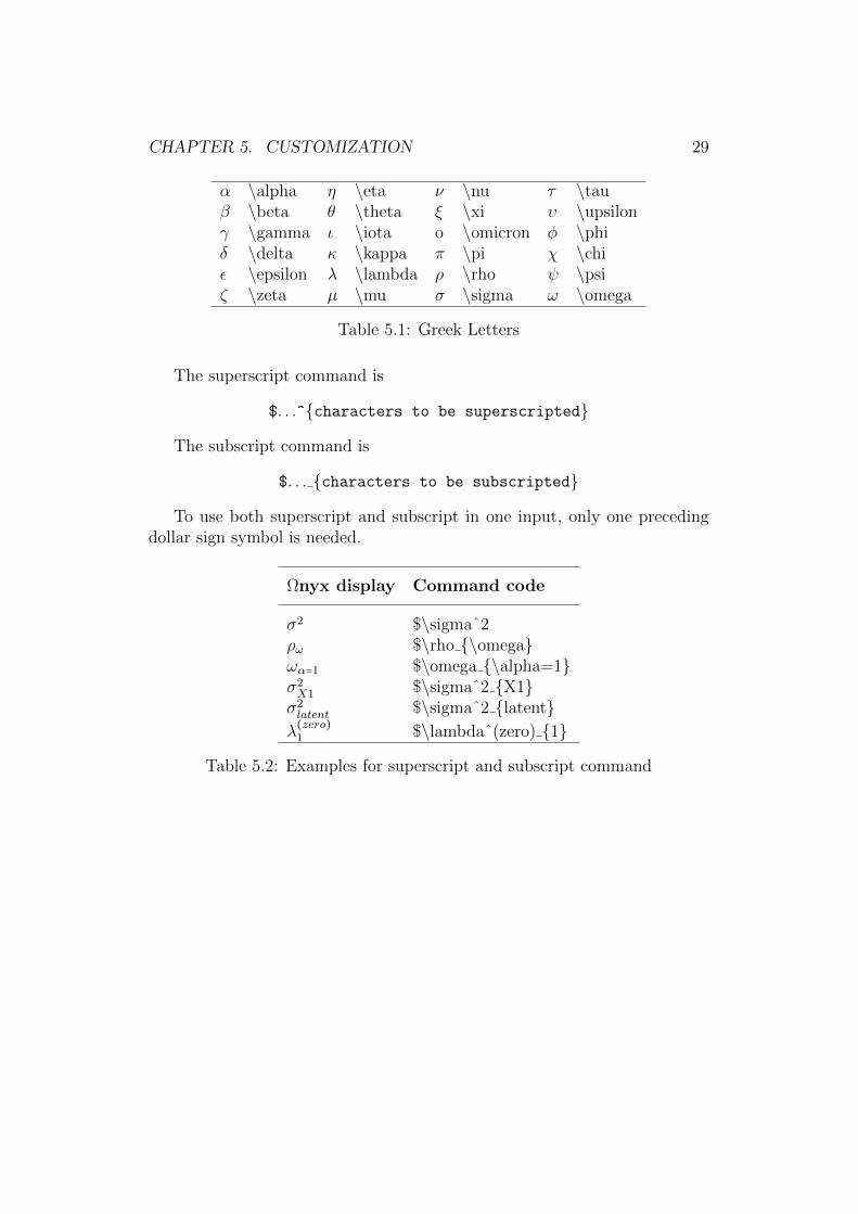
Greek letters It is possible to display Greek letters as parameter names inΩnyx . Type the corresponding codes in the text edit field (see Section 3.3).

Superscripts & subscripts Ωnyx supports a pseudo LaTex input. Bothsuperscript and subscript commands are preceded by a dollar sign symbol($).


Figure 5.5: Customize path styles

Figure 5.6: Customize path styles


α \alpha η \eta ν \nu τ \tauβ \beta θ \theta ξ \xi υ \upsilonγ \gamma ι \iota o \omicron φ \phiδ \delta κ \kappa π \pi χ \chiε \epsilon λ \lambda ρ \rho ψ \psiζ \zeta µ \mu σ \sigma ω \omega

Table 5.1: Greek Letters

The superscript command is

$. . .^characters to be superscripted

The subscript command is

$. . . characters to be subscripted

To use both superscript and subscript in one input, only one precedingdollar sign symbol is needed.

Ωnyx display Command code

σ2 $\sigmaˆ2ρω $\rho \omegaωα=1 $\omega \alpha=1σ2X1 $\sigmaˆ2 X1σ2latent $\sigmaˆ2 latentλ(zero)1 $\lambdaˆ(zero) 1

Table 5.2: Examples for superscript and subscript command

Appendix A

Keyboard Shortcuts

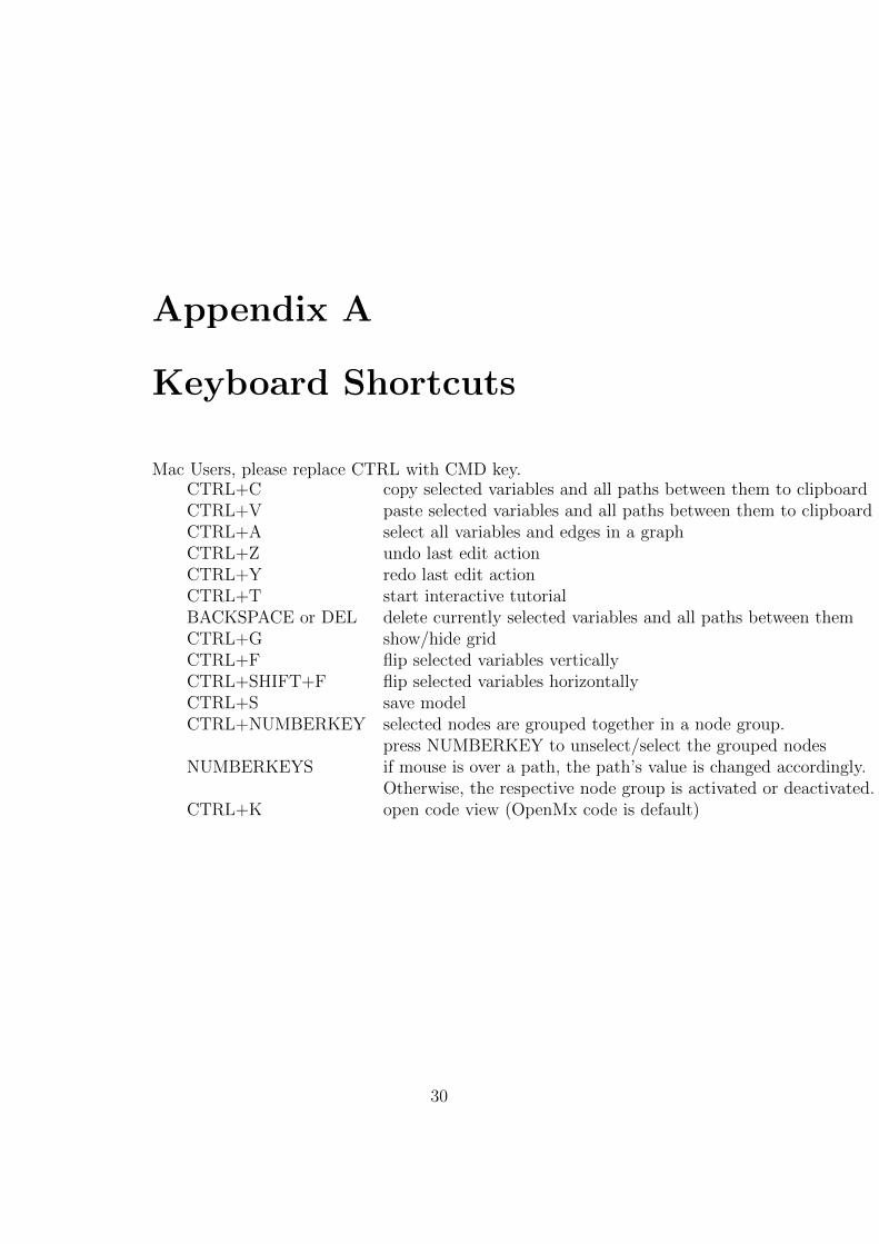
Mac Users, please replace CTRL with CMD key.CTRL+C copy selected variables and all paths between them to clipboardCTRL+V paste selected variables and all paths between them to clipboardCTRL+A select all variables and edges in a graphCTRL+Z undo last edit actionCTRL+Y redo last edit actionCTRL+T start interactive tutorialBACKSPACE or DEL delete currently selected variables and all paths between themCTRL+G show/hide gridCTRL+F flip selected variables verticallyCTRL+SHIFT+F flip selected variables horizontallyCTRL+S save modelCTRL+NUMBERKEY selected nodes are grouped together in a node group.

press NUMBERKEY to unselect/select the grouped nodesNUMBERKEYS if mouse is over a path, the path’s value is changed accordingly.

Otherwise, the respective node group is activated or deactivated.CTRL+K open code view (OpenMx code is default)

30

Ωnyx User Guide

Documents

Transcript of Ωnyx User Guide