NumericalAnalysis-FDMmathsci.kaist.ac.kr/~dykwak/Courses/Num665-09/ch1FDM.pdf ·...
47
Numerical Analysis -FDM D.Y. Kwak September 16, 2014
Transcript of NumericalAnalysis-FDMmathsci.kaist.ac.kr/~dykwak/Courses/Num665-09/ch1FDM.pdf ·...
Numerical Analysis -FDM
D.Y. Kwak
September 16, 2014

ii
Chapter 1
Finite Difference Method
1.1 2nd order linear p.d.e. in two variables
General 2nd order linear p.d.e. in two variables is given in the following form:
L[u] = Auxx + 2Buxy + Cuyy +Dux + Euy + Fu = G, in Ω
where Ω is an open set in R2. According to the relations between coefficients, the
p.d.es are classified into 3 categories, namely,
elliptic if AC −B2 > 0, A, C has the same sign and B is smallhyperbolic if AC −B2 < 0parabolic if AC −B = 0
Furthermore, if the coefficients A,B and C are constant, it can be written as
[∂
∂x,∂
∂y]
[
A BB C
] [∂u∂x∂u∂y
]
+Dux + Euy + Fu = G.
Auxiliary condition
B.C. - Dirichlet, Neumann, Robin
I.C.
Interface Cond
The condition u = g0 on Γ0 ⊂ ∂Ω is called the Dirichlet B.C., the condition∂u∂n = g1 on Γ1 ⊂ ∂Ω is called the Neumann B.C., the condition α∂u
∂n + u =g2 on Γ2 ⊂ ∂Ω is called the Robin B.C. If some of these conditions are mixed, wesay it is a mixed B.C.
1
2 CHAPTER 1. FINITE DIFFERENCE METHOD
Dirichlet Problem
In general a 2nd order linear p.d.e. in Rd can be given in the following convenient
form:
L[u] = −∑di,j=1
∂∂xi
(
aij∂u∂xj
)
+ cu = −∇ · A∇u+ cu = f in Ω
BC’s(1.1)
A = (aij)di,j=1 is the coefficient matrix. The equation will be elliptic if A is
positive definite. Here u maybe electromagnetic potential, displacement of elasticmembrane, temperature, concentration of chemical component, or pressure of afluid(in porous media), etc.
Notations
∂iu =∂u
∂xi, ∂iju =
∂2u
∂xj∂xi,∆ = (∂11 + · · · ∂dd)
so that
∇u = (∂1u, · · · , ∂du)T , ∇ · v = (∂1v1 + · · ·+ ∂dvd)
represent, and a new vector field.
∆ : Laplace operator = ∇ · ∇ = ∇2
C(Ω), C1(Ω), C(Ω), Ck(Ω), C(∂Ω)
• behavior near boundary
• Equation (1.1) holds in an open set Ω.
Definition 1.1.1 (Classical solution). Assume f ∈ C(Ω), g ∈ C(∂Ω). A functionu is called a classical solution if ∈ C2(Ω) ∩ C(Ω).
We say a pde is “well posed” if a solution exists and the solution depends con-tinuously on the data. There are basically two class of method to discretize it,
(1) Finite Difference method
(2) Finite Element method
1.2. FINITE DIFFERENCE METHOD 3
1.2 Finite Difference Method
Let u(x) be a function defined on Ω ⊂ Rn. Let Ui,j be the function defined over
discrete domain (xi, yj) (such points are grid points) that may approximateui,j = u(xi, yj). Such functions are called grid functions.
Difference operator
∂+Ui =Ui+1 − Ui
hi+1, forward difference
∂−Ui =Ui − Ui−1
hi, backward difference
∂0Ui =Ui+1 − Ui−1
hi + hi+1, central difference
∂2Ui =2(∂+ − ∂−)
hi + hi+1, central 2nd difference
Example 1.2.1. Note that
∂+Ui =Ui+1 − Ui
hi+1= ∂0Ui+1/2, central difference at xi+1/2
∂−Ui =Ui − Ui−1
hi= ∂0Ui−1/2, central difference at xi−1/2
H.W 1. We can interpret ∂2Ui as a central difference 2∂0Ui+1/2−∂0Ui−1/2
hi+hi+1. De-
rive the truncation error.
Example 1.2.2. Consider the following second order two point boundary valueproblem :
−u′′(x) = f(x), u(a) = c, u(b) = d.
Assume a mesh a = x0 < x1 < · · · < xN = b,∆xi = xi+1−xi = h. Replacing thederivative by a difference quotient, we obtain
−ui−1 − 2ui + ui+1
h2+O(h2) = f(xi), i = 1, · · ·N − 1, u0 = c, uN = d
Dropping the error term, we obtain a system of linear equations in the approxi-mate values Ui:
−Ui−1 − 2Ui + Ui+1
h2= fi = f(xi), i = 1, · · ·N − 1, U0 = c, UN = d.
4 CHAPTER 1. FINITE DIFFERENCE METHOD
This is an (N − 1)× (N − 1) matrix equations.
h−2
2 −1−1 2 −1
. . .−1 2 −1
−1 2
U1
···
UN−1
=
f1···
fN−1
+ h−2
c000d
Above equation can be written as LhUh = F h, where Uh = (U1, · · · , UN−1)
and F h = (fi) + boundary terms. It is called a difference equation for a givendifferential equation.
Exercise 1.2.3. Write down a matrix equation for the same problem with secondboundary condition changed to the normal derivative condition at b, i.e, u′(b) = d.If one uses first order difference for derivative, we lose accuracy.
We need an extra equation in this case. There are several choices:
(1) Use first order backward difference scheme
UN − UN−1
h= d
and append this to the last eq.( first order)
(2) Assume the D.E. holds at the end point and use central difference equationby using a fictitious point UN+1 :
− 1
h2(UN−1 − 2UN + UN+1) = f(1) (1.2)
1
2h(UN+1 − UN−1) = d (1.3)
Substitute the last eq. into first eq., we have
UN − UN−1
h2=
d
h+
f(1)
2. (1.4)
The matrix is still symmetric; Eq. (1.4) can be viewed as centered differ-ence approximation to u′(xn − h
2 ) and rhs as the first two terms of Taylorexpansion
u′(xn − h
2) = u′(xn)−
h
2u′′(xn) + · · ·
1.2. FINITE DIFFERENCE METHOD 5
g1
g2
x1 x2 x3 x7
x4 x5 x6 x8
b b b
b b b
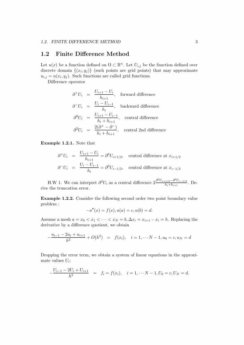
Figure 1.1: Grid for the Neumann problem
(3) Approximate u′(1) by higher order scheme such as
uN−2 − 4uN−1 + 3uN2h
= d.
In this case one has second order truncation error (Show it) but the matrixloses symmetry.
Exercise 1.2.4. (1) Solve above D.E. (Dirichlet and Neumann) with f = 2−6x so that u = x − x2 + x3 and the following BCs (with h = 1/n, n =5, 10, 20, 40). Report the error ‖u− uh‖∞ = maxi |(u− uh)(xi)|.
(a) u(0) = 0, u(1) = 1
(b) u(0) = 0, u′(1) = 2
(2) Write down the stiffness matrix of 2D problem with Neumann conditionat x = 1 on the unit square with 3 × 3 grid. Label the node x1, x2, x3lexicographically from the bottom row.(excluding the boundary) There aretwo possibilities to treat the Neumann condition: One is to use finite differ-ence (backward difference or central differece). Another is to use five pointstencil even at the boundary point with fictitious value and use central dif-ference to extrapolate the fictitious value by u7−u2
2h = g2(1,13 ). Thus from
the stencil, the third equation becomes
1
h2(−2u2 + 4u3 − u6) = (f +
2
hg2)(1,
1
3).
Write down the stiffness matrix of 2D problem with Neumann condition at x = 1on the unit square with 3 × 3 grid. Label the node x1, x2, x3 lexicographicallyfrom the bottom row.(excluding the boundary) There are two possibilities: One
6 CHAPTER 1. FINITE DIFFERENCE METHOD
is same as one dim case at the boundary. Another is to use five point stencileven at the boundary point with fictitious value and use central difference toextrapolate the fictitious value by u7−u2
2h = g2(1,13). Thus the stencil of the third
equation is 1h2 (−2u2 + 4u3 − u5) = f + 1
h2 g2(1,13 ).
Example 1.2.5 (Heat equation). We consider
ut = σuxx, for 0 < x < 1, 0 < t < Tu(t, 0) = u(t, 1) = 0u(0, x) = g(x), g(0) = g(1) = 0
Let xi = ih, i = 0, · · · , N,∆x = 1/N and tn = n∆t,∆t = TJ . Then we have the
following difference scheme
Un+1i − Un
i
∆t= σ
[
Uni−1 − 2Un
i + Uni+1
∆x2
]
,
for i = 1, 2, · · · , N − 1 and n = 1, 2, · · · ,M − 1 where Uni ≈ u(ti, xn). From the
boundary condition and initial condition we have
U0i = g(xi), U
n0 = 0, Un
N = 0.
Un+1i = Un
i +σ∆t
∆x2[
Uni−1 − 2Un
i + Uni+1
]
.
In vector notation
Un+1h = Un
h − σ∆t
∆x2AUn
h
where A is the same matrix as in example 1. If n = 0, right hand side is known.Thus
Unh = (I − σ
∆t
∆x2A)nG, G = (g(x1), · · · , g(xN−1))
T .
This is called forward Euler or explicit scheme. If we change the right handside to
Un+1i − Un
i
∆t= σ
[
Un+1i−1 − 2Un+1
i + Un+1i+1
∆x2
]
Un+1i = Un
i +σ∆t
∆x2[
Un+1i−1 − 2Un+1
i + Un+1i+1
]
.
(I + σ∆t
∆x2A)nUn
h = G, G = (g(x1), · · · , g(xN−1))T .
This is called backward Euler or implicit scheme.
1.2. FINITE DIFFERENCE METHOD 7
1.2.1 Error of difference operator
For u ∈ C2, use the Taylor expansion about xi
ui+1 = u(xi + hi) = u(xi) + hiu′(xi) +
h2i2u′′(ξ), ξ ∈ (xi, xi+1)
∴
ui+1 − uihi
− u′(xi) =hi2u′′(ξ).
Expanding u(xi) about xi+1,
u(xi) = u(xi+1)− hiu′(xi+1) +
h2i2u′′(xi+1)−
h3i6u′′′(θ).
These are first order accurate. To derive a second order scheme, expand aboutxi+1/2,
ui+1 = ui+1/2 +hi2u′(xi+1/2) +
1
2(hi2)2u′′(xi+1/2) +
1
6(hi2)3u(3)(ξ)
ui = ui+1/2 −hi2u′(xi+1/2) +
1
2(hi2)2u′′(xi+1/2)−
1
6(hi2)3u(3)(ξ).
Subtracting, we obtain
ui+1 − uihi
= u′(xi+1/2) +h2i24
u(3)xi+1/2 +O(h3i ).
Thus we obtain a second order approximation to u′(xi+1/2). By translation, wehave
ui+1 − ui−1
2hi− u′(xi) = O(h2i /6) if hi = hi+1. (1.5)
H.W. Do the same for irregular mesh.(use weighted difference)Assume hi = hi+1 and we substitute the solution of differential equation into
the difference equation. Using −u′′ = f we obtain
(−ui−1 + 2ui − ui+1)
h2− f(xi) := Lhu− F h
=1
h2(−ui + hu′i −
h2
2u′′i +
h3
6u(3) − h4
24u(4)(θ1) + 2ui)
+1
h2(−ui − hu′i −
h2
2u′′i −
h3
6u(3) − h4
24u(4)(θ2))− f(xi)
= −u′′i − f(xi)−h2
24(u(4)(θ1) + u(4)(θ2))
=h2
24max |u(4)|.
8 CHAPTER 1. FINITE DIFFERENCE METHOD
Thus we obtain a discrete equation
LhU = F h. (1.6)
We let τh = Lhu− F h and call it the truncation error.
Definition 1.2.6. We say a difference scheme is consistent if the truncationerror approaches zero as h approaches zero, in other words, if Lhu − f → 0 insome norm.
Truncation error measures how well the difference equation approximates thedifferential equation. But it does not measure the actual error in the solution.
Use of different quadrature for f . Instead of f(xi) we can use
1
12[f(xi−1) + 10f(xi) + f(xi+1)] =
5
6f(xi) +
µ0
6f(xi)
where µ0f(xi) is the average of f which is f(xi) +O(h2).H.W. Show for uniform grid, we have
−ui−1 + 2ui − ui−1
h2=
1
12[f(xi−1) + 10f(xi) + f(xi+1)] + Ch4 max |u(6)(x)|.
Nonuniform grid(irregular mesh)
We use central difference scheme at xi±1/2 to get
u′(xi+1/2) ≈ ui+1−ui
hi+1and u′(xi−1/2) ≈ ui−ui−1
hi.
Thus, it is natural to define
u′′(xi) ≈ (ui+1 − ui
hi+1− ui − ui−1
hi)/(
hi + hi+1
2).
H.W. Find truncation error for of difference scheme for −u′′(xi) − f in caseof nonuniform grid.
Lhu− f = 2[−hiui+1 + (hi + hi+1)ui − hi+1ui−1]/hihi+1(hi + hi+1)− f(xi)
= 2
[
−hi(ui + hi+1u′i +
h2i+1
2u′′i +
h3i+1
6u(3)i +O(h4)) + (hi + hi+1)ui
−hi+1(ui − hiu′i +
h2i2u′′i −
h3i6u(3)i +O(h4))
]
/hihi+1(hi + hi+1)− f(xi)
= −u(2)i − fi +
1
3(hi+1 − hi)u
(3)i +O(h2i + h2i+1).
H.W Use 13 [f(xi) + f(xi+1) + f(xi−1)] for the right hand side. What is the
truncation error?
1.3. ELLIPTIC EQUATION 9
Definition 1.2.7. Lh is said to be stable if there is a constant C independentof h such that
‖Uh‖ ≤ C‖F h‖ for all h > 0
where Uh is the solution of the difference equation, LhUh = F h. In other word,
Lh is stable if and only if L−1h is bounded.
Definition 1.2.8. A finite difference scheme is said to converge if
‖Uh − u‖ → 0 as h → 0.
eh = Uh − u is called the discretization error.
Theorem 1.2.9 (P. Lax). Given a consistent scheme, stability is equivalent toconvergence.
Proof . Assume stability. From Lhu− f = τh, LhUh − F h = 0, we have Lh(u−
Uh) = τh. Thus,
‖u− Uh‖ ≤ C‖Lh(u− Uh)‖ = C‖τh‖ → 0.
Hence the scheme converges. Obviously a convergent scheme must be stable.From the theory of p.d.e, we know ‖u‖ ≤ C‖f‖. Hence
‖Uh‖ ≤ ‖Uh − u‖+ ‖u‖ ≤ O(τh) + C‖f‖ ≤ C‖f‖ ≤ C‖F h‖.
1.3 Elliptic equation
1.3.1 Basic finite difference method for elliptic equation
In this chapter, we only consider finite difference method. First consider thefollowing elliptic problem:(Dirichlet problem by Finite Difference Method)
−∆u = f in Ωu = g on ∂Ω
(1) Approx. D.E. −(uxx+uyy) = f by a finite difference at each interior meshpt.
(2) The unknown function u is approximated by a grid function Uh
10 CHAPTER 1. FINITE DIFFERENCE METHOD
u(x+ h) = u(x) + hux(x) +h2
2 uxx(x) +h3
6 uxxx(x) +O(h4)u(x− h) = . . .
u(x+ h)− 2u(x) + u(x− h)
h2= uxx(x) +O(h2)
uxx(x, y).= [u(x+ h, y)− 2u(x, y) + u(x− h, y)]/h2
uyy(x, y).= [u(x, y + h)− 2u(x, y) + u(x, y − h)]/h2
××
×
×
(x− h, y) (x, y) (x+ h, y)
(x, y − h)
(x, y + h)
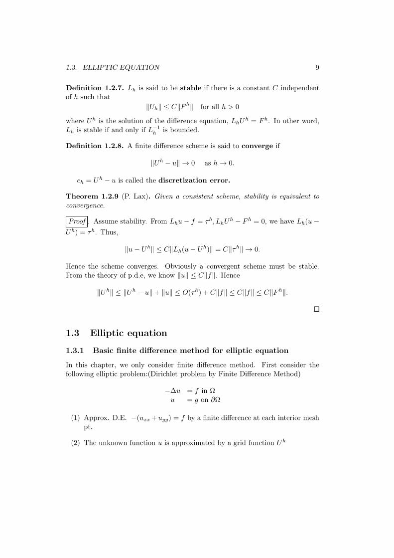
Figure 1.2: 5-point Stencil
This picture is called, Molecule, Stencil, Star, etc. For each point (interiormesh pt), approx ∇2u = ∆u by 5-point stencil. By Girshgorin disc theorem, thematrix is nonsingular. L[u] is called differential operator while Lh[u] is calledfinite difference operator, e.g.,
Lh[u](x, y) = [−4u(x, y) + u(x+ h, y) +u(x− h, y) +u(x, y+h) +u(x, y−h)]/h2
or more generally,
L[u] = −[∂
∂x,∂
∂y] Diaga11, a22
[∂u∂x∂u∂y
]
+ cu = −(a11ux)x − (a22uy)y + cu
With uniform meshes
ux(x).= u(x+h)−u(x−h)
2h
(ux)x(x).=
ux(x+h2)−ux(x−
h2)
h Central difference
Note thatux(x+ h
2 ) =u(x+h)−u(x)h
ux(x− h2 ) =u(x)−u(x−h)
h
1.3. ELLIPTIC EQUATION 11
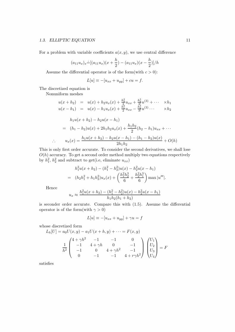
For a problem with variable coefficients a(x, y), we use central difference
(a11ux)x=[(a11ux)(x+h
2)− (a11ux)(x− h
2)]/h
Assume the differential operator is of the form(with c > 0):
L[u] ≡ −[uxx + uyy] + cu = f.
The discretized equation isNonuniform meshes
u(x+ h2) = u(x) + h2ux(x) +h222 uxx +
h323! u
(3) + · · · ×h1
u(x− h1) = u(x)− h1ux(x) +h212 uxx − h3
23! u
(3) · · · ×h2
h1u(x+ h2)− h2u(x− h1)
= (h1 − h2)u(x) + 2h1h2ux(x) +h1h22
(h2 − h1)uxx + · · ·
∴ ux(x) =h1u(x+ h2)− h2u(x− h1)− (h1 − h2)u(x)
2h1h2+O(h)
This is only first order accurate. To consider the second derivatives, we shall loseO(h) accuracy. To get a second order method multiply two equations respectivelyby h21, h
22 and subtract to get(i.e, eliminate uxx)
h21u(x+ h2)− (h21 − h22)u(x) − h22u(x− h1)
= (h2h21 + h1h
22)ux(x) +
(
h21h32
6+
h22h31
6
)
max |u′′′|.
Hence
ux ≈ h21u(x+ h2)− (h21 − h22)u(x)− h22u(x− h1)
h1h2(h1 + h2)
is seconder order accurate. Compare this with (1.5). Assume the differentialoperator is of the form(with γ > 0)
L[u] ≡ −[uxx + uyy] + γu = f
whose discretized formLh[U ] = a0U(x, y)− a1U(x+ h, y) + · · · = F (x, y)
1
h2
4 + γh2 −1 −1 0−1 4 + γh 0 −1−1 0 4 + γh2 −10 −1 −1 4 + rγh2
U1
U2
U3
U4
= F
satisfies
12 CHAPTER 1. FINITE DIFFERENCE METHOD
(1) Lh[u] = L[u] +O(h2) as h → 0. u is true solution.
(2) AU = F +Bdy, Au = [∆u− γu+O(h2)] +Bdy
With abuse of notation, we have
Lh(U − u) = O(h2) = τh
Let A be the matrix representation of Lh then with abuse of notations. thediscretization error U − u has the form A−1τh(depends on h) and satisfies
‖U − u‖ ≤ ‖A−1‖ · ‖τh‖ ≤ ‖A−1‖O(h2)
If we put D = diagA = a11, . . . , ann, then D−1A(U − u) = D−1τh. WriteD−1A = I + B, where B is off diagonal. Then we know ‖B‖∞ = 4
4+γh2 < 1 if
γ > 0. Thus (D−1A)−1 = (I +B)−1 exists and
‖(D−1A)−1‖∞ = ‖(I +B)−1‖∞ ≤ 1
1− ‖B‖∞≤ 4 + γh2
γh2.
Hence
‖U − u‖∞ ≤ ‖(D−1A)−1‖∞ · ‖D−1τh‖∞ ≤ 4 + γh2
γh2· h2
4 + γh2O(h2) = O(h2) → 0
Thus, we have proved the following result.
Theorem 1.3.1 (Convergence of FDM -special case). Let
(1) u ∈ C4(Ω)
(2) γ > 0
(3) uniform mesh
Then ‖U − u‖∞ = O(h2) as h → 0.
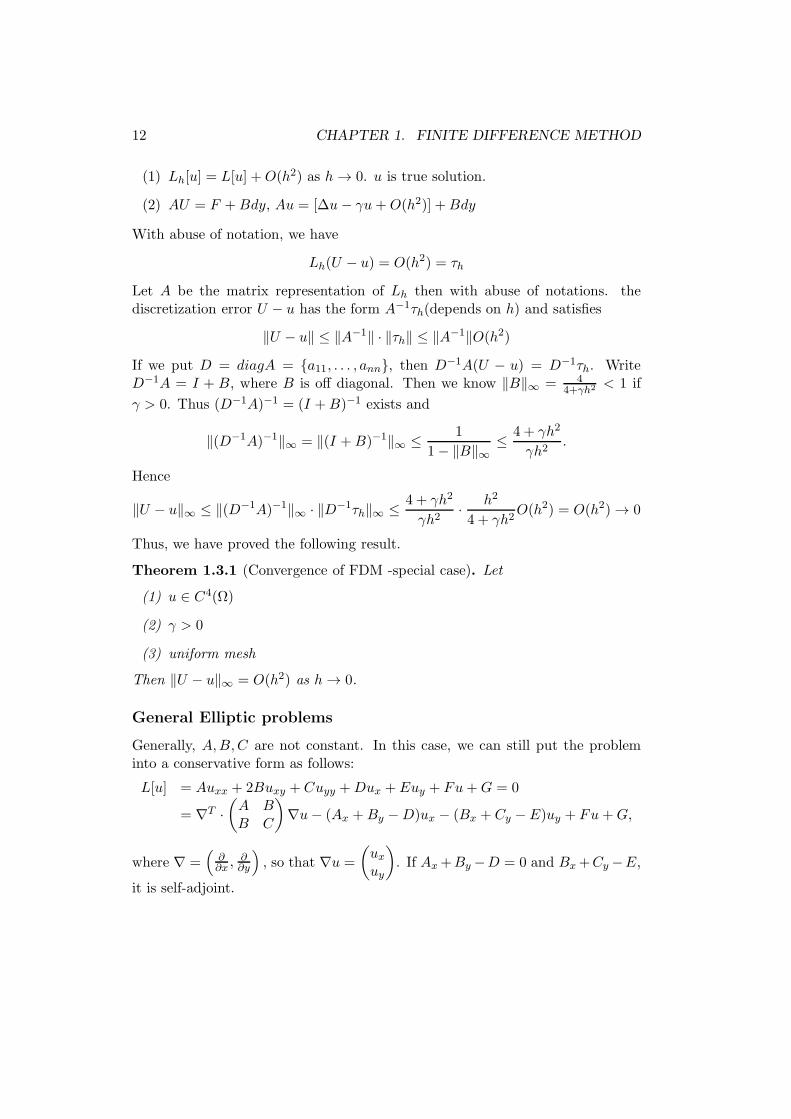
General Elliptic problems
Generally, A,B,C are not constant. In this case, we can still put the probleminto a conservative form as follows:
L[u] = Auxx + 2Buxy + Cuyy +Dux + Euy + Fu+G = 0
= ∇T ·(
A BB C
)
∇u− (Ax +By −D)ux − (Bx + Cy − E)uy + Fu+G,
where ∇ =(
∂∂x ,
∂∂y
)
, so that ∇u =
(
uxuy
)
. If Ax+By −D = 0 and Bx+Cy −E,
it is self-adjoint.
1.3. ELLIPTIC EQUATION 13
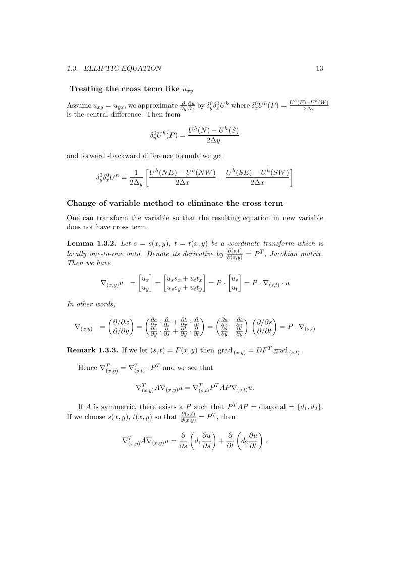
Treating the cross term like uxy
Assume uxy = uyx, we approximate ∂∂y
∂u∂x by δ0yδ
0xU
h where δ0xUh(P ) = Uh(E)−Uh(W )
2∆xis the central difference. Then from
δ0yUh(P ) =
Uh(N)− Uh(S)
2∆y
and forward -backward difference formula we get
δ0yδ0xU
h =1
2∆y
[
Uh(NE)− Uh(NW )
2∆x− Uh(SE)− Uh(SW )
2∆x
]
Change of variable method to eliminate the cross term
One can transform the variable so that the resulting equation in new variabledoes not have cross term.
Lemma 1.3.2. Let s = s(x, y), t = t(x, y) be a coordinate transform which is
locally one-to-one onto. Denote its derivative by ∂(s,t)∂(x,y) = P T , Jacobian matrix.
Then we have
∇(x,y)u =
[
uxuy
]
=
[
ussx + uttxussy + utty
]
= P ·[
usut
]
= P · ∇(s,t) · u
In other words,
∇(x,y) =
(
∂/∂x∂/∂y
)
=
( ∂s∂x · ∂
∂s +∂t∂x · ∂
∂t∂s∂y · ∂
∂s +∂t∂y · ∂
∂t
)
=
( ∂s∂x
∂t∂x
∂s∂y
∂t∂y
) (
∂/∂s∂/∂t
)
= P · ∇(s,t)
Remark 1.3.3. If we let (s, t) = F (x, y) then grad (x,y) = DF T grad (s,t).
Hence ∇T(x,y) = ∇T
(s,t) · P T and we see that
∇T(x,y)A∇(x,y)u = ∇T
(s,t)PTAP∇(s,t)u.
If A is symmetric, there exists a P such that P TAP = diagonal = d1, d2.If we choose s(x, y), t(x, y) so that ∂(s,t)
∂(x,y) = P T , then
∇T(x,y)A∇(x,y)u =
∂
∂s
(
d1∂u
∂s
)
+∂
∂t
(
d2∂u
∂t
)
.
14 CHAPTER 1. FINITE DIFFERENCE METHOD
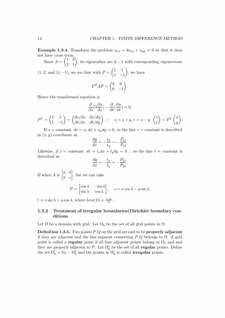
Example 1.3.4. Transform the problem uxx + 4uxy + uyy = 0 so that it doesnot have cross term.
Since A =
(
1 22 1
)
, its eigenvalues are 3,−1 with corresponding eigenvectors
(1, 1) and (1,−1), we see that with P =
(
1 11 −1
)
, we have
P TAP =
(
3 00 −1
)
.
Hence the transformed equation is
∂
∂s(3∂u
∂s)− ∂
∂t(∂u
∂t) = 0.
P T =
(
1 11 −1
)
=
(
∂s/∂x ∂s/∂y∂t/∂x ∂t/∂y
)
. ∴ s = x+ y, t = x− y.
(
st
)
= P T
(
xy
)
.
If s = constant, ds = sx dx+ sy dy = 0, so the line s = constant is describedin (x, y)-coordinate as
dy
dx= −sx
sy= −P11
P12.
Likewise, if t = constant, dt = txdx + tydy = 0 ∴ so the line t = constant isdescribed as
dy
dx= − tx
ty= −P21
P22.
If when A is
[
a bb c
]
, the we can take
P =
[
cos λ − sinλsinλ cos λ
]
, s = x cos λ− y sinλ,
t = x sinλ+ y cos λ, where b cot 2λ = c−a2 .
1.3.2 Treatment of irregular boundaries(Dirichlet boundary con-ditions
Let Ω be a domain with grid. Let Ωh be the set of all grid points in Ω.
Definition 1.3.5. Two points P,Q on the grid are said to be properly adjacent
if they are adjacent and the line segment connecting P,Q belongs to Ω. A gridpoint is called a regular point if all four adjacent points belong to Ωh and andthey are properly adjacent to P . Let Ω∗
h be the set of all regular points. Definethe set Ω′
h = Ωh − Ω∗h and the points in Ω′
h is called irregular points.
1.3. ELLIPTIC EQUATION 15
×
×
×
×
×
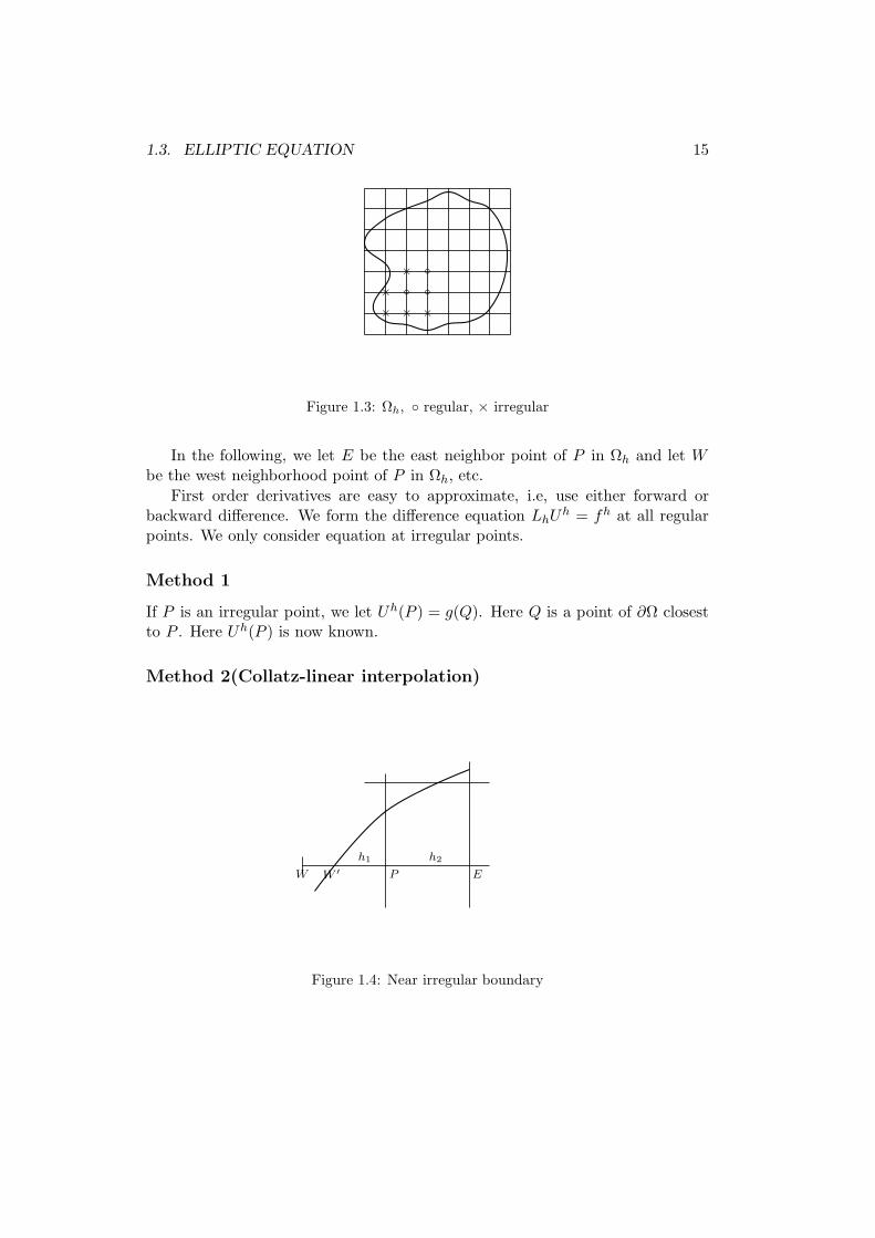
Figure 1.3: Ωh, regular, × irregular
In the following, we let E be the east neighbor point of P in Ωh and let Wbe the west neighborhood point of P in Ωh, etc.
First order derivatives are easy to approximate, i.e, use either forward orbackward difference. We form the difference equation LhU
h = fh at all regularpoints. We only consider equation at irregular points.
Method 1
If P is an irregular point, we let Uh(P ) = g(Q). Here Q is a point of ∂Ω closestto P . Here Uh(P ) is now known.
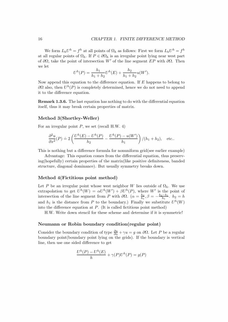
Method 2(Collatz-linear interpolation)
W W ′ P E
h1 h2
Figure 1.4: Near irregular boundary
16 CHAPTER 1. FINITE DIFFERENCE METHOD
We form LhUh = fh at all points of Ωh as follows: First we form LhU
h = fh
at all regular points of Ωh. If P ∈ ∂Ωh is an irregular point lying near west partof ∂Ω, take the point of intersection W ′ of the line segment EP with ∂Ω. Thenwe let
Uh(P ) =h1
h1 + h2Uh(E) +
h2h1 + h2
u(W ′).
Now append this equation to the difference equation. If E happens to belong to∂Ω also, then Uh(P ) is completely determined, hence we do not need to appendit to the difference equation.
Remark 1.3.6. The last equation has nothing to do with the differential equationitself, thus it may break certain properties of matrix.
Method 3(Shortley-Weller)
For an irregular point P , we set (recall H.W. 4)
∂2u
∂x2(P )
.= 2
(
Uh(E)− Uh(P )
h2− Uh(P )− u(W ′)
h1
)
/(h1 + h2), etc..
This is nothing but a difference formula for nonuniform grid(see earlier example)
Advantage: This equation comes from the differential equation, thus preserv-ing(hopefully) certain properties of the matrix(like positive definiteness, bandedstructure, diagonal dominance). But usually symmetry breaks down.
Method 4(Fictitious point method)
Let P be an irregular point whose west neighbor W lies outside of Ωh. We useextrapolation to get Uh(W ) = αUh(W ′) + βUh(P ), where W ′ is the point ofintersection of the line segment from P with ∂Ω. (α = h2
h1, β = −h2−h1
h1. h2 = h
and h1 is the distance from P to the boundary.) Finally we substitute Uh(W )into the difference equation at P . (It is called fictitious point method)
H.W. Write down stencil for these scheme and determine if it is symmetric!
Neumann or Robin boundary condition(regular point)
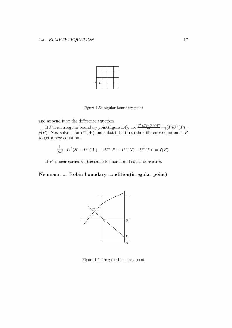
Consider the boundary condition of type ∂u∂n + γu = g on ∂Ω. Let P be a regular
boundary point(boundary point lying on the grids). If the boundary is verticalline, then use one sided difference to get
Uh(P )− Uh(E)
h+ γ(P )Uh(P ) = g(P )
1.3. ELLIPTIC EQUATION 17
P E
Figure 1.5: regular boundary point
and append it to the difference equation.
If P is an irregular boundary point(figure 1.4), use Uh(E)−Uh(W )2h +γ(P )Uh(P ) =
g(P ). Now solve it for Uh(W ) and substitute it into the difference equation at Pto get a new equation.
1
h2(−Uh(S)− Uh(W ) + 4Uh(P )− Uh(N)− Uh(E)) = f(P ).
If P is near corner do the same for north and south derivative.
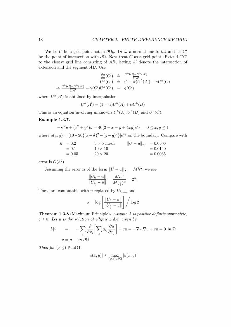
Neumann or Robin boundary condition(irregular point)
C′
C B
A
A′
Figure 1.6: irregular boundary point
18 CHAPTER 1. FINITE DIFFERENCE METHOD
We let C be a grid point not in ∂Ωh. Draw a normal line to ∂Ω and let C ′
be the point of intersection with ∂Ω. Now treat C as a grid point. Extend CC ′
to the closest grid line consisting of AB, letting A′ denote the intersection ofextension and the segment AB. Use
∂u∂n(C
′).= Uh(C)−Uh(A′)
CA′
Uh(C ′).= (1− σ)Uh(A′) + γUh(C)
⇒ Uh(C)−Uh(A′)
CA′+ γ(C ′)Uh(C ′) = g(C ′)
where Uh(A′) is obtained by interpolation.
Uh(A′) = (1− α)Uh(A) + αUh(B)
This is an equation involving unknowns Uh(A), Uh(B) and Uh(C).
Example 1.3.7.
−∇2u+ (x2 + y2)u = 40(2 − x− y + 4xy)exy, 0 ≤ x, y ≤ 1
where u(x, y) = [10−20(x− 12 )
2+(y− 12)
2]exy on the boundary. Compare with
h = 0.2 5× 5 mesh ‖U − u‖∞ = 0.0506= 0.1 10× 10 = 0.0140= 0.05 20× 20 = 0.0035
error is O(h2).
Assuming the error is of the form ‖U − u‖∞ = Mhα, we see
‖Uh − u‖‖Uh
2− u‖ =
Mhα
M(h2 )α= 2α.
These are computable with u replaced by Uhminand
α = log
[
‖Uh − u‖‖Uh
2− u‖
]
/
log 2
Theorem 1.3.8 (Maximum Principle). Assume A is positive definite symmetric,c ≥ 0. Let u is the solution of elliptic p.d.e. given by
L[u] = −∑
i
∂
∂xi
[
∑
j
aij∂u
∂xj
]
+ cu = −∇A∇u+ cu = 0 in Ω
u = g on ∂Ω
Then for (x, y) ∈ int Ω
|u(x, y)| ≤ max(x,y)∈∂Ω
|u(x, y)|
1.3. ELLIPTIC EQUATION 19
Proof . Assume c > 0. There exists orthogonal matrix P such that P TAP =
diagd1, d2 where d1, d2 > 0. If u has a positive maximum at some interior pointQ = (x∗, y∗) of Ω, then define
(
st
)
= P T (x∗, y∗)
(
xy
)
so that L[u] = −∇(s,t)PTAP∇(s,t)u + cu = 0. At Q, us(Q) = ut(Q) = 0,
uss(Q) ≤ 0 and utt(Q) ≤ 0. Hence
L[u] = −(d1us)s(Q)− (d2ut)t(Q) + c(Q)u(Q) = 0
Recall d1 > 0, d2 > 0, cu > 0, we see this is a contradiction. Thus either
0 ≤ u(x∗, y∗) ≤ max(x,y)∈∂Ω
u(x, y)
or u(x, y) ≤ u(x∗, y∗) < 0 for all (x, y). Similarly, u cannot have negative mini-mum.
Now if c ≥ 0 we consider a perturbation. Choose α so large that L[eαx] =−(d1α
2 + d2α2 − c)eαx < 0 and let v = u+ Eeαx.
L[v] = L[u] +EL[eαx] < 0 for all E > 0.
Suppose v has a pos. max. at Q, an interior point of Ω. Then L[v] = −d1vss(Q)−d2vtt(Q) + c(Q)v(Q) ≥ 0, a contradiction. Hence u(x, y) ≤ v(x, y) < max∂Ωu+Eeαx. Let E → 0. Then
u(x, y) ≤ max∂Ω
u.
Remark 1.3.9. Examining above proof we can conclude L[u] = 0 can be replacedby L[u] ≤ 0.
Applying maximum principle to u and −u, we see u cannot have negativeminimum, i.e,
u(x, y) ≥ min∂Ω
u.
Thus, we obtain the result.
Corollary 1.3.10. If
L[u] = 0 in Ω
u = 0 on ∂Ω,
then u ≡ 0.
20 CHAPTER 1. FINITE DIFFERENCE METHOD
As a consequence we have uniqueness of solution.
Corollary 1.3.11. If u1, u2 satisfy
L[ui] = f in Ω
ui = g on ∂Ω,
then u1 = u2.
Remark 1.3.12. Examining the proof, one can notice slight weaker version ofMaximum principle holds if L(u) ≤ 0. Under the same condition as previoustheorem, except L(u) ≤ 0, we see u cannot have positive maximum in the interior.
H.W. State and prove a version of minimum principle.
Theorem 1.3.13 (Discrete max. principle). Let the grid function U satisfy thefinite difference equation Lh[U ] ≡∑QA(P,Q)U(Q) = 0, i.e,
A(P,P )U(P )+A(P,E)U(E)+A(P, S)U(S)+A(P,N)U(N)+A(P,W )U(W ) = 0
for each mesh point P , where coefficient A(P,Q) are generated by finite differencemethod and A is pos. def. weakly diagonally dominant.
Then|U(P ∗)| ≤ max
P∈∂Ωh
|U(P )|, for all P∗ ∈ intΩh. (1.7)
Proof . Solving for U(P ), we have
U(P ) = 1A(P,P )
∑
Q 6=P
−A(P,Q)U(Q)
Since |A(P,P )| ≥∑
Q 6=P
|A(P,Q| we have
|U(P )| ≤∑
Q 6=P
∣
∣
∣
∣
A(P,Q)
A(P,P )
∣
∣
∣
∣
maxQ 6=P
|U(Q)| ≤ maxQ 6=P
|U(Q)|.
Repeat the same process until you hit the boundary.
Corollary 1.3.14 (Uniqueness of discrete solution).
LhU = 0 in ΩU = 0 on ∂Ω
implies U = 0.
1.3. ELLIPTIC EQUATION 21
Theorem 1.3.15 (Discrete max. principle 2nd version). Suppose Lh[U ] ≤ 0Then U cannot have a positive maximum unless U is constant. In other words,
0 < maxp∈Ωh
U(p) = max∂Ωh
U(p)
or
maxp∈Ωh
U(p) < 0
Proof . Suppose there is a point P0 ∈ Ωh such that U(P0) is positive and U(P0) ≥U(P ) for all P ∈ Ωh. Then by similar argument as above,
U(P0) ≤∑
Q 6=P0
∣
∣
∣
∣
A(P0, Q)
A(P0, P0)
∣
∣
∣
∣
maxQ 6=P0
U(Q) ≤ maxQ 6=P0
U(Q) ≤ U(P0).
Hence
U(Q) = U(P0)
for all Q in the nhd of P0. Repeating the argument for each Q in the nhd of P0
until we hit the boundary, we see U must be constant. Thus we have the desiredresult.
Note. Minimum principle is obtained when Lh[U ] ≥ 0.
Theorem 1.3.16 (Convergence of FDM - More general case). Let u be the so-lution of L[u] = −∇TA∇u + cu = 0 in Ω and u = g on ∂Ω and let U be thefinite sequence of grid functions satisfying LhU = 0, where Lh(u) = O(hα),α > 0(truncation error). If A is constant, diagonally dominant, positive definite,then ‖U − u‖∞ = O(hα) as h → 0.
Proof . Let w = U − u, then Lh[w] = Lh[U ] − Lh[u] = −Lh[u] and w = 0 on
∂Ω. Let s(x, y) ≡ r2 − (x − x0)2 − (y − y0)
2 with (x0, y0) ∈ intΩ, r chosen solarge that the circle s = 0 contains Ω. Then Lh[s] = L[s] because s is quadratic.(compute it)
L[s] = −∇TA∇s+ cs = −a11sxx − (a12 + a21)sxy − a22syy + cs= 2(a11 + a22) + cs ≥ 2(a11 + a22).
There exist M > 0 such that |Lh[u]| ≤ Mhα by the hypothesis Lh[u] = O(hα).We see that
Lh
[
Mhαs(x, y)
2(a11 + a22)
]
≥ Mhα ≥ |Lh[u]|.
22 CHAPTER 1. FINITE DIFFERENCE METHOD
Also
Lh
[
±w − Mhαs(x, y)
2(a11 + a22)
]
= ±Lh[w]− Lh[ ] ≤ ∓Lh[u]−Mhα ≤ 0
(Recall w = U − u and Lh[w] = −Lh[u] and w = 0 on ∂Ω)Now by the discrete maximum principle-2nd version (where Lh(U) = 0 is
replaced by Lh[U ] ≤ 0),
maxP∈Ωh
[
±w − Mhαs
2(a11 + a22)
]
≤ maxP∈∂Ωh
[
±w − Mhαs
2(a11 + a22)
]
= − Mhα
2(a11 + a22)min∂Ωh
s ≤ 0.
Thus |w| ≤ Mhαs2(a11+a22)
and
‖u− U‖∞ = ‖w‖∞ ≤ Mhα
2(a11 + a22)maxΩ
s ≤ Mhαr2
2(a11 + a22).
1.3.3 Convection -diffusion equation
Consider another type of differential equation, namely a special case of convectiondiffusion equation.
−ǫuxx + aux = f
u(0) = u0, u(1) = u1
or with Neumann condition u′(1) = 0 if a(1) > 0. Here, we assume 0 < ǫ << 1.If we use the central difference scheme for the first order derivative, we get
ǫ
(
−Uhi−1 + 2Uh
i − Uhi+1
h2
)
+ aUhi+1 − Uh
i−1
2h= fh
i
−( ǫ
h2+
a
2h
)
Uhi−1 +
2ǫ
h2Uhi −
( ǫ
h2− a
2h
)
Uhi+1 = fh
i
Thus the sum of off diagonal elements is∑
j 6=i
|aij | =∣
∣
∣
ǫ
h2+
a
2h
∣
∣
∣+∣
∣
∣
ǫ
h2− a
2h
∣
∣
∣ .
If a, h is fixed and ǫ → 0, it becomes a/h, while aii = 2ǫ/h2 → 0. Thus theresulting matrix is not diagonally dominant and it causes a lot of problems. Forexample, the resulting linear system is not positive definite and hence it may bemore difficult to solve. But, most importantly, the resulting discretization doesnot yield an accurate approximation to the problem. One way to fix this situationis to keep the Peclet number : ah
ǫ < 2 so that the sum of off diagonal elements isless than or equal to 2ǫ/h2 = aii. The disadvantage of this scheme is that smallh enlarges the size of discrete equation.
1.3. ELLIPTIC EQUATION 23
Numerical Difficulties
(1) The solution may exhibit oscillation which are physically unrealistic
(2) Taking small mesh size means large problem size which take more time tosolve.
(3) The iterative method may fail to converge
Upwind difference scheme
An alternative way to avoid this difficulty is to use backward difference for ux fora > 0 and forward difference for ux for a < 0. This method of choosing differencescheme is called upwind difference scheme. For a > 0
ǫ
(
−Uhi−1 + 2Uh
i − Uhi+1
h2
)
+ aUhi − Uh
i−1
h= fh
i
−( ǫ
h2+
a
h
)
Uhi−1 +
(
2ǫ
h2+
a
h
)
Uhi −
( ǫ
h2
)
Uhi+1 = fh
i
The resulting system is irreducibly diagonally dominant, thus it is an M -matrix.Error analysis can be carried out to show optimal order of convergence. Also, forthe solver part, simple Jacobi method works.
Example 1.3.17.
−ǫu′′ + u′ = 0 in (0, 1)
with u(0) = 0, u(1) = ǫ(1− e−1ǫ ) has unique solution u(x) = −ǫe−
xǫ + ǫ.
The following examples are taken from (K.W. Morton-Numerical Solution ofconvection-Diffusion problems, Chapman Hall, 1996)
Example 1.3.18.
−ǫ∆u+ b · ∇u = 0 on (0, 1) × (0, 1)
with
b = b(cos θ, sin θ)
for 0 ≤ θ < π2 and discontinuous inflow boundary condition
u(0, y) =
0, y ∈ [0, 12)1, y ∈ (12 , 1]
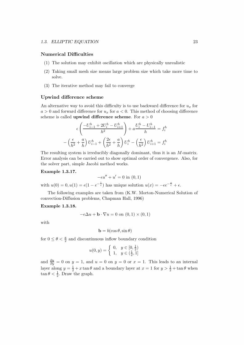
and ∂u∂y = 0 on y = 1, and u = 0 on y = 0 or x = 1. This leads to an internal
layer along y = 12 + x tan θ and a boundary layer at x = 1 for y > 1
2 +tan θ whentan θ < 1
2 . Draw the graph.
24 CHAPTER 1. FINITE DIFFERENCE METHOD
u = 0
u = 1
∂u∂n
= 0
u = 0
u = 0
y = 12+ x tan θ
Figure 1.7: internal and boundary layer
Example 1.3.19 (Heat equation).
∂u
∂t+ b · ∇u = ǫ∆u on (−1, 1) × (−1, 1) × (0, T )
u(x, y, 0) = u0(x, y)
where u0(x, y) is a circular cone type centered at (1, 0) with
b = b(wy,−wx)
with exact inflow boundary where needed.
H.W Construct a 2-D example with exact solution exhibiting some (boundary)layer.
u = (exǫ − 1)(e
yǫ − 1)
An example of exact solution of heat equation(nonseparable) is the fundamentalsolution(shifted):
u =1
√
4π(t+ 1)e− x2
4(t+1)
1.4 Parabolic p.d.e’s
Consider a heat equation on a bar.
ut = uxx, 0 ≤ x ≤ 1, 0 < t ≤ T.
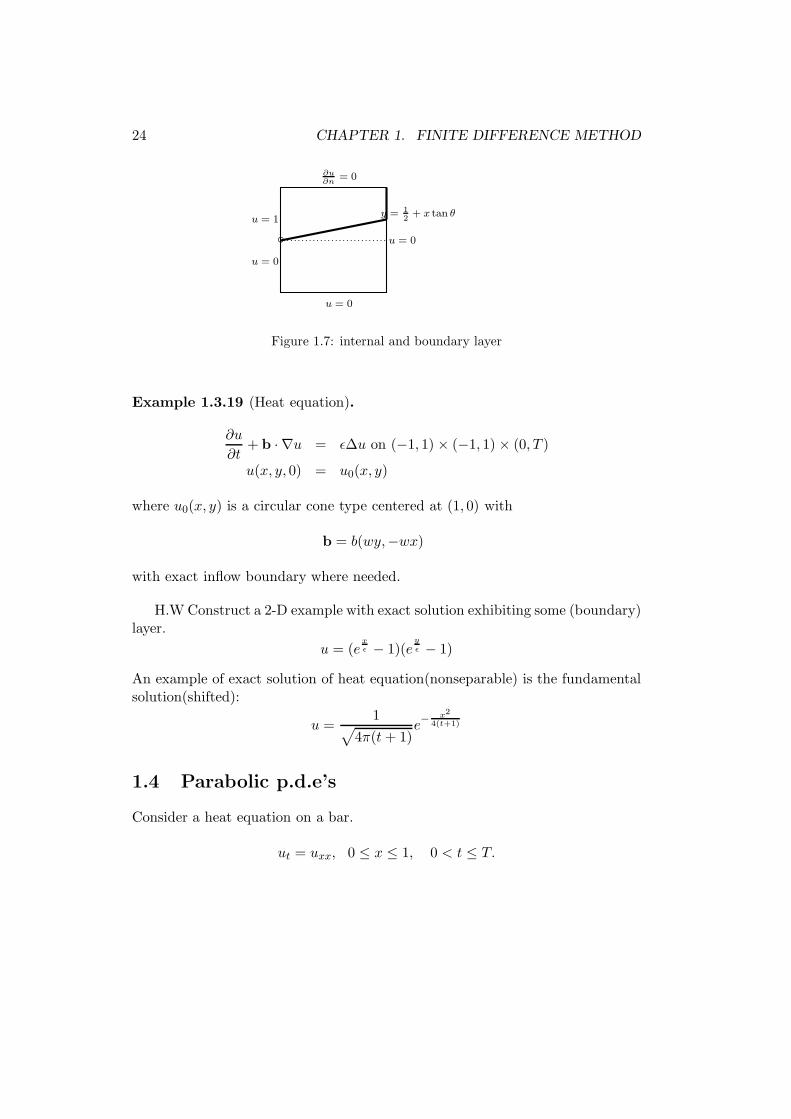
1.4. PARABOLIC P.D.E’S 25
1f(x)
g(t) h(t)
T
Ω
Figure 1.8: Domain
Theorem 1.4.1 (Maximum principle). If u satisfies the heat equation for t ≤ T ,then
minf, g, h = m ≤ min0≤x≤1,0≤t≤T
u ≤ max0≤x≤1,0≤t≤T
u ≤ M = maxf, g, h
Proof . Put v = u+Ex2, E > 0
∂v
∂t− ∂2v
∂x2= −2E < 0
If v attains a maximum at Q ∈ int Ω, then
vt(Q) = 0,vxx(Q) ≤ 0.
Thus (vt − vxx)(Q) ≥ 0, a contradiction. Hence v has maximum at a boundarypoint of Ω
u(x, t) ≤ v(x, t) ≤ max v(x, t) ≤ M + E.
Since E was arbitrary, the proof is complete. For minimum, use −E instead ofE.
More general parabolic p.d.e.
ut = Auxx +Dux + Fu+G
F.D.M
Explicit · · ·write down the values of grid function
Implicit · · · variables implicitly representing the value
Let the grid be given by
0 = x0 < x1 < x2 < · · · < xN+1 = 1, xi = ih, uniform grid
0 = t0 < t1 < · · · , tj = jk
26 CHAPTER 1. FINITE DIFFERENCE METHOD
Explicit method
Ui,j+1−Ui,j
k.= ut
Ui+1,j−2Ui,j+Ui−1,j
h2
.= uxx
∴ Ui,j+1 = λUi−1,j + (1− 2λ)Ui,j + λUi+1,j
where λ = k/h2.Recall: Stability means solution remains bounded as time goes on.
Theorem 1.4.2. If u is sufficiently smooth, then∣
∣
∣
∣
uxx −u(x+ h, t)− 2u(x, t) + u(x− h, t)
h2
∣
∣
∣
∣
= O(h2) as h → 0
and∣
∣
∣
∣
ut −u(x, t+ k)− u(x, t)
k
∣
∣
∣
∣
= O(k) as k → 0
Theorem 1.4.3. Suppose u is sufficiently smooth, and satisfies
ut = uxx 0 < x < 1, t > 0u(x, 0) = f(x)u(0, t) = g(t)u(1, t) = h(t).
If Ui,j is the solution of the explicit finite difference scheme, then for 0 < λ ≤ 12 ,
maxi, j
|ui,j − Ui,j| .= O(h2 + k) as h, k → 0,
i.e, finite difference solution converges to the true solution.
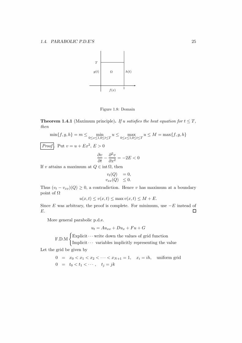
Proof . Put uij ≡ u(xi, tj). Then from
h 2h 3h 4h
u = g1(y) u = g2(y)
u = f(x)
Figure 1.9:
1.4. PARABOLIC P.D.E’S 27
(1)ui,j+1 − ui,j
k= ut +O(k)
(2)ui+1,j − 2ui,j + ui−1,j
h2= uxx +O(h2)
we get
ui,j+1 = ui,j +k
h2(ui+1,j − 2ui,j + ui−1,j) + k(O(k) +O(h2)).
Henceui,j+1 = λui−1,j + (1− 2λ)ui,j + λui+1,j + Ck(k + h2).
Let the discretization error be wi,j = uij − Uij so that
wi,j+1 = λwi−1,j + (1− 2λ)wi,j + λwi+1,j +O(k2 + kh2).
Since 0 < λ ≤ 12 , 0 ≤ 1 − 2λ < 1, three coefficient are positive and their sum is
1. (convex combination) We see
|wi,j+1| ≤ λ|wi−1,j |+(1−2λ)|wi,j |+λ|wi+1,j |+M(k2+kh2) for some M > 0.
If we define ‖wj‖ = max1≤i≤N |wi,j|, then
‖wj+1‖ ≤ ‖wj‖+M(k2 + kh2)≤ ‖wj−1‖+ 2M(k2 + kh2) ≤ · · · ≤ ‖w0‖+ (j + 1)M(k2 + kh2).
Since ‖w0‖ = 0,
‖wj+1‖ ≤ (j + 1)kM(k + h2) ≤ TM(k + h2), (j + 1)k ≤ T.
In fact,
M = max0≤x≤1, 0≤t≤T
(1
2|utt|+
1
12|uxxxx|).
Remark 1.4.4. If λ > 12 , the solution may not converge.
Exercise 1.4.5. Prove the formula is unstable for λ > 12 . Let
u(x, 0) =
ε, x = 12
0, x 6= 12
with g = h = 0
Ui,j+1 = λUi−1,j + (1− 2λ)Ui,j + λUi+1,j , λ = k/h2
|Ui,j+1| = λ|Ui−1,j|+ (2λ− 1)|Ui,j |+ λ|Ui+1, j|, 1 ≤ i ≤ N − 1.
28 CHAPTER 1. FINITE DIFFERENCE METHOD
Here the equality holds because the sign of Ui alternates, so the three terms havethe same sign. Hence
N−1∑
i=1
|Ui,j+1| = λ
N−1∑
i=1
|Ui−1,j |+ (2λ− 1)
N−1∑
i=1
|Ui,j |+ λ
N−1∑
i=1
|Ui+1,j|.
Since U(xi, t) = 0, i = 1, N , we can add them and
N−1∑
i=1
|Ui,j+1| = λ
N−2∑
i=0
|Ui,j|+ (2λ− 1)
N−1∑
i=1
|Ui,j |+ λ
N∑
i=2
|Ui,j|.
Let S(tj) =∑N
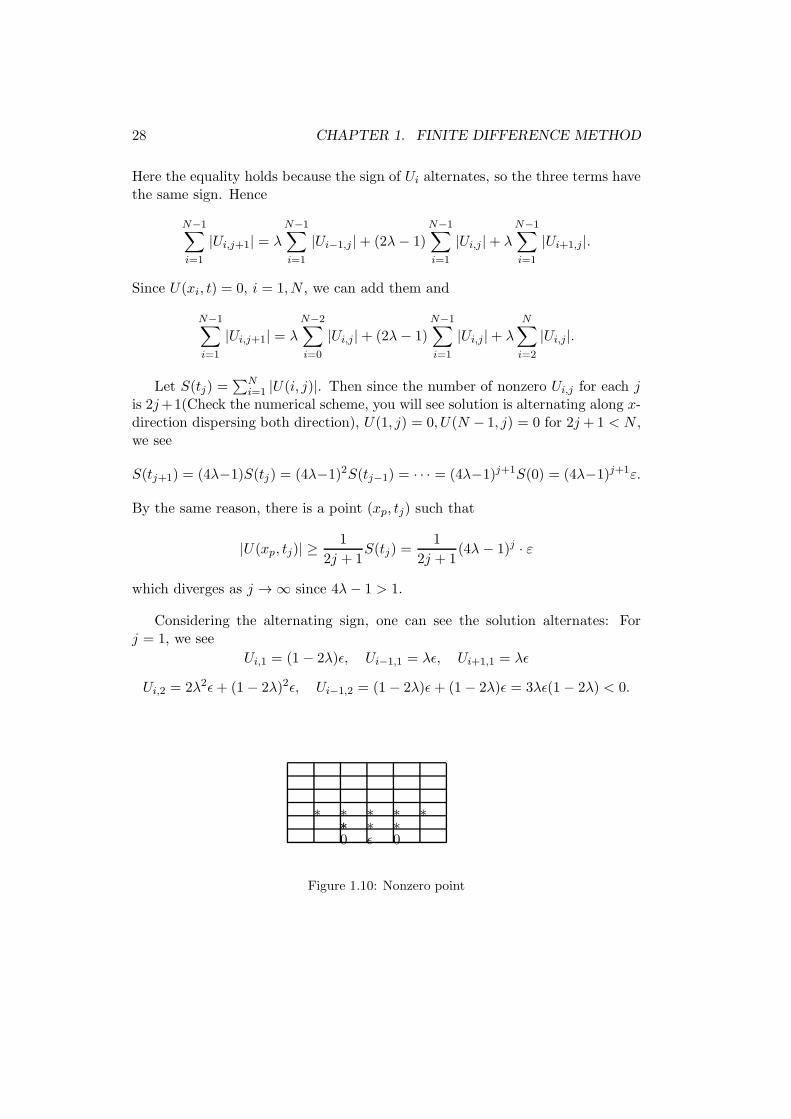
i=1 |U(i, j)|. Then since the number of nonzero Ui,j for each jis 2j+1(Check the numerical scheme, you will see solution is alternating along x-direction dispersing both direction), U(1, j) = 0, U(N − 1, j) = 0 for 2j +1 < N ,we see
S(tj+1) = (4λ−1)S(tj) = (4λ−1)2S(tj−1) = · · · = (4λ−1)j+1S(0) = (4λ−1)j+1ε.
By the same reason, there is a point (xp, tj) such that
|U(xp, tj)| ≥1
2j + 1S(tj) =
1
2j + 1(4λ− 1)j · ε
which diverges as j → ∞ since 4λ− 1 > 1.
Considering the alternating sign, one can see the solution alternates: Forj = 1, we see
Ui,1 = (1− 2λ)ǫ, Ui−1,1 = λǫ, Ui+1,1 = λǫ
Ui,2 = 2λ2ǫ+ (1− 2λ)2ǫ, Ui−1,2 = (1− 2λ)ǫ+ (1− 2λ)ǫ = 3λǫ(1− 2λ) < 0.
0 ǫ 0∗ ∗ ∗∗
∗ ∗∗ ∗ ∗
Figure 1.10: Nonzero point
1.4. PARABOLIC P.D.E’S 29
Stability of linear system
U1,j+1...
UN−1,j+1
=
1− 2λ λ . . . 0
λ 1− 2λ. . .
0. . . λλ 1− 2λ
U1,j...
UN−1,j
+
g(tj)0...0
h(tj)
In vector form, Uj+1 = AUj +Gj. Assume Gj = 0, j = 1, 2, . . . . Let µ be aneigenvalue of A. Then by G-disk theorem,
|1− 2λ− µ| ≤ 2λ
−2λ ≤ 1− 2λ− µ ≤ 2λ
−2λ ≤ −1 + 2λ+ µ ≤ 2λ
1− 4λ ≤ µ ≤ 1
If 0 < λ ≤ 12 , then −1 ≤ µ ≤ 1, hence stable. If λ > 1
2 , then |µ| > 1 is possible. Sothe scheme may be unstable. The following example show it is actually unstable.
Example 1.4.6 (Issacson, Keller). Try v(x, t) = Re(eiαx−wt) = cosαx · e−wt.
vt − vxx.=
v(x, t+∆t)− v(x, t)
∆t− v(x+∆x, t)− 2v(x, t) + v(x−∆x, t)
∆x2
= v(x, t)
(
e−w∆t − 1
∆t
)
− cos(αx+ α∆x)− 2 cosαx+ cos (αx− α∆x)
∆x2e−wt
= v(x, t)
(
e−w∆t − 1
∆t− 2 cosα∆x− 2
∆x2
)
= v(x, t)1
∆te−w∆t − [(1 − 2λ) + 2λ cosα∆x]
= v(x, t)1
∆t
[
e−w∆t −(
1− 4λ sin2α∆x
2
)]
Thus v is a solution of the difference equation provided w and α satify e−w∆t =1− 4λ sin2 α∆x
2 .With I.C. v(x, 0) = cosαx, solution becomes
v(x, t) = cosαxe−wt = cosαx
(
1− 4λ sin2α∆x
2
) t∆t
Clearly, for all λ ≤ 12 , |v(x, t)| ≤ 1. However, if λ > 1
2 , then for some ∆x, wehave
∣
∣1− 4λ sin2 α∆x2
∣
∣ > 1. So v(x, t) becomes arbitrarily large for sufficiently
30 CHAPTER 1. FINITE DIFFERENCE METHOD
large t/∆t. Since every even function has a cosine series, we may express any evenfunction f(x) in the form f(x) =
∑
n αn cos(απx) to get an unstable problem.(Seebook for details)
Implicit Finite Difference Method.
Given a heat equation
ut = uxxu(0, t) = g(t), t > 0u(1, t) = h(t)u(x, 0) = f(x), 0 ≤ x ≤ 1.
We discretize it by implicit difference method.
Ui,j+1 − Ui,j
∆t=
Ui+1,j+1 − 2Ui,j+1 + Ui−1,j+1
∆x2i = 1, . . . , N − 1.
Multiply by ∆t, then with λ = ∆t/∆x2, we have
Ui,j+1 − Ui,j = λUi+1,j+1 − 2λUi,j+1 + λUi−1,j+1
−Ui,j = λUi+1,j+1 − (1 + 2λ)Ui,j+1 + λUi−1,j+1 j = 1, . . . , N − 1.
This yields a system of N − 1 unknowns in Ui,j+1N−1i=1 .
−λU0,j+1
0...0
−λUN,j+1
+
−U1,j...
−UN−1,j
= −
(1 + 2λ) −λ 0
−λ (1 + 2λ) −λ
0. . .
. . .. . .
. . .. . . −λ
0 −λ (1 + 2λ)
×
U1,j+1...
UN−1,j+1
Theorem 1.4.7. The implicit finite difference scheme is stable for all λ =∆t/∆x2. (The solution remains bounded).
Proof . For each j, let Uk(j),j be chosen so that |Uk(j),j| ≥ |Ui,j|, i = 1, . . . , N−1.
We choose i0 = k(j + 1) in the following relation.
Ui,j+1 = Ui,j + λUi+1,j+1 − 2Ui,j+1 + Ui−1,j+1.
1.4. PARABOLIC P.D.E’S 31
Then(1 + 2λ)Ui0,j+1 = Ui0,j + λUi0+1,j+1 + Ui0−1,j+1
for 1 ≤ i ≤ N − 1. Taking absolute values,
(1 + 2λ)|Ui0,j+1| ≤ |Ui0,j|+ λ(|Ui0+1,j+1|+ |Ui0−1,j+1|) ≤ |Ui0,j|+ 2λ|Ui0,j+1|.
Thus |Ui0,j+1| ≤ |Ui0,j| ≤ |Uk(j),j| and hence |Ui,j+1| ≤ |Ui0,j+1| ≤ |Uk(j),j | for1 ≤ i ≤ N − 1. Repeat the same procedure until j = 0.
|Ui,j+1| ≤ |Uk(j),j| ≤ · · · ≤ |Uk(0),0| ≤ M = max(f, g, h), for 1 ≤ i ≤ N − 1.
Since |Ui,j+1| ≤ M = maxf, g, h, for i = 0 or N , the relation holds for all i.
Using the matrix formulation: We check the eigenvalues of the system
AUj+1 = Uj +Gj
Eigenvalue of A satisfies |µ + (1 + 2λ)| ≤ 2λ by G-disk theorem. From this, wesee |µ| ≥ 1 and hence the eigenvalues of A−1 is less than one in absolute value.Thus
Uj+1 ≤ A−1(Uj+Gj) = · · · = A−j−1U0+A−j−1G0+A−j−2G1+ · · ·+A−1Gj.
‖Uj+1‖ ≤ ‖A−j−1‖ ‖U0‖+ ‖A−1‖ · 1
1− ‖A−1‖ maxj
‖Gj‖
remain bounded. Note. A does not have−1 as eigenvalues and all the eigenvaluesare positive real.
Theorem 1.4.8. For sufficiently smooth u, we have
|uij − Uij | = O(h2 + k) as h and k → 0 (for all λ)
Proof . Let uij = u(xi, tj) be the true solution. Then we have
ui,j+1 − ui,jk
=1
h2ui+1,j+1 − 2ui,j+1 + ui−1,j+1+O(h2 + k)
Let wi,j = ui,j − Ui,j be the discretization error. Then
wi,j+1 = wi,j + λwi+1,j+1 − 2wi,j+1 + wi−1,j+1+O(kh2 + k2)(1 + 2λ)wi,j+1 = wi,j + λwi+1,j+1 + λwi−1,j+1 +O(kh2 + k2)
Let ‖wj‖ = maxi |wi,j|. Then for all i
(1 + 2λ)|wi,j+1| ≤ ‖wj‖+ 2λ‖wj+1‖+O(kh2 + k2)
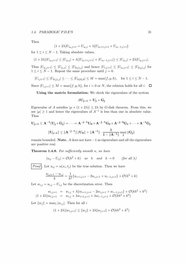
32 CHAPTER 1. FINITE DIFFERENCE METHOD
t = j
t = j + 1
ui−1,j
ui,j
ui+1,j
ui,j+1
ui−1,j+1
ui,j+1
ui+1,j+1
ui,j
Figure 1.11: Stencil for forward, backward Euler method
and so(1 + 2λ)‖wj+1‖ ≤ ‖wj‖+ 2λ‖wj+1‖+O(kh2 + k2).
Thus
‖wj+1‖ ≤ ‖wj‖+ C(kh2 + k2)
≤ · · · ≤ ‖w0‖+ C(j + 1)k(k + h2)
≤ ‖w0‖+ CT (k + h2) = CT (k + h2)
for t = (j + 1)k ≤ T .
1.4.1 Discretization of parabolic p.d.e, General Case
Consider
c∂u
∂t=
∂
∂x(p
∂u
∂x) +
∂
∂y(p
∂u
∂y)− γu+ f in Ω× [0, T ]
I.C. u(x, y, 0) = h(x, y) in Ω
B.C. u(x, y, t) = g(x, y, t) for (x, y) ∈ ∂Ω.
where c, p, γ, f are functions of x, y and t. Assume
0 < p0 ≤ p(x, y, t) ≤ p10 ≤ γ(x, y, t) ≤ γ
0 < c0 ≤ c(x, y, t) ≤ c1.
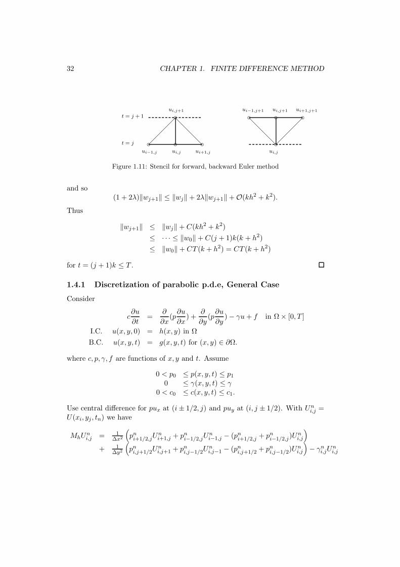
Use central difference for pux at (i± 1/2, j) and puy at (i, j ± 1/2). With Uni,j =
U(xi, yj , tn) we have
MhUni,j = 1
∆x2
(
pni+1/2,jUni+1,j + pni−1/2,jU
ni−1,j − (pni+1/2,j + pni−1/2,j)U
ni,j
)
+ 1∆y2
(
pni,j+1/2Uni,j+1 + pni,j−1/2U
ni,j−1 − (pni,j+1/2 + pni,j−1/2)U
ni,j
)
− γni,jUni,j
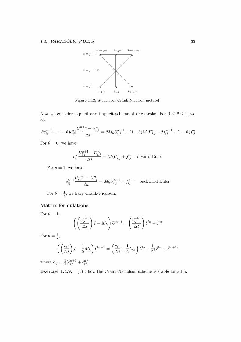
1.4. PARABOLIC P.D.E’S 33
t = j
t = j + 1/2
t = j + 1
ui−1,j
ui,j
ui+1,j
ui−1,j+1
ui,j+1
ui+1,j+1
Figure 1.12: Stencil for Crank-Nicolson method
Now we consider explicit and implicit scheme at one stroke. For 0 ≤ θ ≤ 1, welet
[θcn+1ij + (1− θ)cnij]
Un+1i,j − Un
i,j
∆t= θMhU
n+1i,j + (1− θ)MhU
ni,j + θfn+1
ij + (1− θ)fnij
For θ = 0, we have
cnijUn+1i,j − Un
i,j
∆t= MhU
ni,j + fn
ij forward Euler
For θ = 1, we have
cn+1ij
Un+1i,j − Un
i,j
∆t= MhU
n+1i,j + fn+1
ij backward Euler
For θ = 12 , we have Crank-Nicolson.
Matrix formulations
For θ = 1,((
cn+1ij
∆t
)
I −Mh
)
~Un+1 =
(
cn+1ij
∆t
)
~Un + ~Fn
For θ = 12 ,
((
cij∆t
)
I − 1
2Mh
)
~Un+1 =
(
cij∆t
+1
2Mh
)
~Un +1
2(~Fn + ~Fn+1)
where cij =12(c
n+1ij + cnij).
Exercise 1.4.9. (1) Show the Crank-Nicholson scheme is stable for all λ.
34 CHAPTER 1. FINITE DIFFERENCE METHOD
(2) With θ = 1/2, the error is O(∆t2 +∆x2).
(3) Consider a heat equation with κ = 1
ut = κuxx 0 < x < 1, t > 0u(x, 0) = f(x)u(0, t) = g(t)u(1, t) = h(t).
where κ > 0 is constant. If f(x) = cos πx, g(t) = e−π2κt, h(t) = −e−π2κt
it has solution u = e−π2κt cos πx. (For nonseparable example, just addlinear function in x or use fundamental solution of heat equation shifted)Use the following method to compute numerical solution up to T = 1.0.Check ‖u− U‖2 or ‖u− U‖∞ for time step j∆t = 0.1, 0.2, 0.3, etc.
(a) Explicit FDM with h = 110 ,
120 , for k = λh2 where λ = 0.2, 0.4 and 0.6.
(b) Implicit FDM with h = 110 ,
120 , for k = λh2 where λ = 0.2, 0.4, 0.6, 0.8
and 1.6 .
(c) Crank-Nicholson scheme
You can use either Gauss-Seidel type of iteration method or LU-decompositionto solve the system of equations arising in the implicit method.
1.4. PARABOLIC P.D.E’S 35
Using central difference at (xi, tj+ 12),
ui,j+1 − ui,jk
= ut(xi, tj+ 12) +O(k2) (1.8)
Using
Mhui,j = uxx(xi, tj) +O(h2) = uxx(xi, tj+ 12)− k
2uxxt(xi, tj+ 1
2) +O(k2 + h2)(1.9)
Mhui,j+1 = uxx(xi, tj+1) +O(h2) = uxx(xi, tj+ 12) +
k
2uxxt(xi, tj+ 1
2) +O(k2 + h2)(1.10)
we see
ui,j+1 − ui,j∆t
= θMhui,j + (1− θ)Mhui,j+1 + ut(xi, tj+ 12)− uxx(xi, tj+ 1
2)(1.11)
+k
2(1− 2θ)uxxt(xi, tj+ 1
2) +O(k2 + h2) (1.12)
Hackbusch book Chap 4. FDM. Chap. 10 singular perturbation, Ch. 11, Eigen-value
Crank-Nicholson again
[θcn+1ij + (1− θ)cnij]
Un+1i,j − Un
i,j
∆t= θMhU
n+1i,j + (1− θ)MhU
ni,j + θfn+1
ij + (1− θ)fnij
(1.13)
ui,j+1 − ui,jk
=1
k(kut(xi, tj) +
1
2k2utt +
1
6k3uttt) (1.14)
Using
Mhui,j = uxx(xi, tj) +O(h2) (1.15)
Mhui,j+1 = uxx(xi, tj+1) +O(h2) (1.16)
= uxx(xi, tj) + uxxt(xi, tj)k +O(k2 + h2) (1.17)
we see
ut(xi, tj) +1
2kutt = uxx(xi, tj) + (1− θ)kutt(xi, tj) +O(k2 + h2) (1.18)
Let τ = Uh − u. Then from (1.13), the truncation error satisfies
τ(x, t) = (1
2− θ)kutt +O(k2 + h2) (1.19)
36 CHAPTER 1. FINITE DIFFERENCE METHOD
1.5 Finite element method for parabolic problems
Let I = (0, T ).
∂u
∂t−∆u = f in Ω× I (1.20)
u = 0 in Γ× I (1.21)
u(x, 0) = u0, in Ω (1.22)
We shall study two methods: Semi-discretization(discretization in space only)and Full-discretization(discretization in time and space).
1.5.1 One dimensional model problem
∂u
∂t− α2 ∂
2u
∂x2= f, (x, t) ∈ (0, L)× I (1.23)
u(0, t) = u(π, t) = 0, t ∈ I (1.24)
u(x, 0) = u0(x), x ∈ (0, L). (1.25)
For simplicity, assume α = 1, L = π and f = 0. Using the periodic B.C., let usexpress u in terms of its Fourier sine series:
u(x, t) =
∞∑
j=1
cje−j2t sin(jx),
where cj =
√
2
π
∫ π
0u0(x) sin(jx) dx. Generally, the solution is given by
u(x, t) =∞∑
j=1
cje−j2πα2t/L sin
(
jπx
L
)
,
cj =
√
2
L
∫ L
0u0(x) sin
(
jπx
L
)
dx. We see that u is a linear combination of
sine waves with amplitude cje−j2t If j2t is large, e−j2t ≈ 0,(i.e, high frequency
component quickly damps out and u(x, t) becomes smoother) which happens ifj is large or t is large. This phenomena is consistent with the nature of diffusionprocess such as heat conduction. However, when t is close to 0, u is not smooth.It is known that
‖ ·u‖L2(0,π) = O(t−s).
1.6. SEMI DISCRETIZATION IN SPACE 37
The nature is like this: The smoother the initial function is, the more rapidly cj
decays as j → ∞. An initial phase when·u is large, is called an initial transient.
This will affect on choosing the time step size. Basic Stability.
‖u(·, t)‖ ≤ ‖u0‖, t ∈ I (1.26)
‖ ·u(·, t)‖ ≤ C
t‖u0‖, t ∈ I. (1.27)
1.6 Semi discretization in space
Let V = H10 (Ω). Multiply the equation by v
(·u(t), v) + a(u(t), v) = (f(t), v), v ∈ V (1.28)
(u(0), v) = (u0, v). (1.29)
Let Vh = Spanφ1, · · · , φN. Then the finite element formulation is
(·uh(t), v) + a(uh(t), v) = (f(t), v) (1.30)
(uh(0), v) = (u0, v), v ∈ Vh. (1.31)
With uh(x, t) =∑N
i=1 ξi(t)φi(x),∑
i
ξ′i(t)(φi, φj) +∑
i
ξi(t)a(φi, φj) = (f(t), φj)
∑
i
ξ(0)(φi, φj) = (u0, φj), j = 1, · · · , N.
In matrix form
B.ξ(t) +Aξ(t) = F (t)
Bξ(0) = U0
where B = (bij), A = (aij), F = (Fj) ξ = (ξi), U0 = (U0
j ). bij = (φj , φi) ,Aij = a(φj , φi)), etc.
Mass matrix B and stiffness matrix A is SPD. κ(B) = O(1), κ(A) = O(h−2).With Cholesky decomposition B = LTL, η = Lξ, we can reduce it as
.η + Aη(t) = g(t) (1.32)
η(0) = η0 (1.33)
where A = L−TAL−1 is also SPD. g = L−TF , η0 = L−TU0. The solution isgiven by
η(t) = e−Atη0 +
∫ t
0e−A(t−s)g(s)ds.
38 CHAPTER 1. FINITE DIFFERENCE METHOD
Stability: Take v = uh(x, t) := uh(t) in (1.30) with f = 0
(·uh(t), uh(t)) + a(uh(t), uh(t)) = 0
1
2
d
dt‖uh(t)‖2 + a(uh(t), uh(t)) = 0
‖uh(t)‖2 + 2
∫ 1
0a(uh(t), uh(t)) = ‖uh(0)‖2 ≤ ‖u0‖2.
In particular,
‖uh(t)‖ ≤ ‖uh(0)‖ ≤ ‖u0‖, t > 0.
Theorem 1.6.1. c There is a constant C such that
maxt∈I
‖u(t)− uh(t)‖ ≤ C
(
1 + lnT
h2
)
maxt∈I
h2‖u(t)‖H2 . (1.34)
1.7 Fully discrete Scheme
We shall now discretize the scheme in time also. Here, we use finite differencemethod to discretize along time while we maintain finite element discretizationalong space. First consider a related problem (1.30).
To see the behavior of η(t), we write
η(t) =
N∑
i=1
(η0, χi)e−µntχi,
where χi is an orthonormal eigenvectors of A,
µ1 ≤, · · · ,≤ µM , µ1 = O(1), µM = O(h−2).
This again has an initial transient. For accuracy, we need to take small time step,or use implicit method.
0 = t0 < t1, · · · , < tN = T, ∆tn = tn − tn−1.
Forward Euler method:
(
un+1h − unh∆tn+1
, v
)
+ a(unh, v) = (f(tn), v), v ∈ Vh, n = 1, 2, · · ·
(u0h, v) = (u0, v).
1.7. FULLY DISCRETE SCHEME 39
Backward Euler method:(
un+1h − unh∆tn+1
, v
)
+ a(un+1h , v) = (f(tn+1), v), v ∈ Vh, n = 1, 2, · · ·(1.35)
(u0h, v) = (u0, v).
Discretization error is O(∆tn). Let uh(x, t) =∑M
i=1 ξi(t)φi(x). Then takingv = φj
(∑
i
ξn+1i φj , φj) + ∆tn+1a(
∑
i
ξn+1i φj , φj) = (
∑
i
ξni φj , φj) + ∆tn+1(f(tn+1), φj)
(1.36)Or
(B +∆tn+1A)ξn+1 = Bξn +∆tn+1F (tn+1). (1.37)
For stability with f = 0, take v = un+1h in (1.35)
(un+1h , un+1
h )− (un+1h , unh) + ∆tn+1a(u
n+1h , un+1
h ) = 0.
Using arithmetic-geometric inequality (u, v) ≤ 12(ǫ‖u‖2 +
‖v‖ǫ )
1
2(‖un+1
h ‖2 − ‖unh‖2) + ∆tn+1a(un+1h , un+1
h ) ≤ 0.
Summing up
‖un+1h ‖2 + 2∆tn+1a(u
n+1h , un+1
h ) ≤ ‖u0h‖2 ≤ ‖u0‖2.
In particular‖un+1
h ‖ ≤ ‖u0h‖ ≤ ‖u0‖, n = 1, 2 · · · (1.38)
Now Crank-Nicholson. We use combination of forward and backward Eulerscheme.
(
un+1h − unh∆tn+1
, v
)
+ a
(
un+1h + unh
2, v
)
=
(
f(tn+1) + f(tn)
2, v
)
, (1.39)
(u0h, v) = (u0, v), v ∈ Vh, n = 1, 2, · · ·
Discetization error is O(∆tn2)
Taking v = (un+1h + unh)/2 we obtain the stability as before. In matrix form
(
B +∆tn+1
2A
)
ξn+1 =
(
B − ∆tn+1
2A
)
ξn +∆tn+1F (tn+1) + F (tn)
2(1.40)
40 CHAPTER 1. FINITE DIFFERENCE METHOD
As in (1.32) we use η = Lξ associated with Cholesky-decomposition, then thetransformed equation becomes
ηn+1 − ηn
∆tn+1+
1
2A(ηn+1 + ηn) =
1
2(g(tn+1) + g(tn)). (1.41)
In case g = 0, we have
(
I +1
2∆tn+1A
)
ηn+1 =
(
I − 1
2∆tn+1A
)
ηn.
and∣
∣
∣
∣
∣
∣
∣
∣
∣
∣
(
I +1
2∆tn+1A
)−1(
I − 1
2∆tn+1A
)
∣
∣
∣
∣
∣
∣
∣
∣
∣
∣
= maxj
|1− 12∆tn+1λj|
1 + 12∆tn+1λj
< 1.
Thus the scheme is stable for all time step ∆tn(unconditionally stable) However,for backward-Euler or Crank-Nicholson method, one has to solve a system oflinear equation for each time step, which is costly.
For the forward Euler method, one can compute ηn+1 directly without solvingany system, but for stability, one has to take small time step. In fact, one canshow that
ηn+1 = (I −∆tn+1A)ηn
and
‖I −∆tn+1A‖ = maxj
|1−∆tn+1λj| ≤ 1
only if ∆tn+1λM ≤ 2 or ∆tn+1 = O(h2) (conditionally stable). Hence for theforward Euler method the stability is guaranteed only when time step is verysmall even for moderate h.
1.8 Hyperbolic Equation
ut + a11ux + a12vx = b1
vt + a21ux + a22vx = b2(1.42)
where ai,j and u, v and function of (x, t).
u(x, 0) = f(x)
v(x, 0) = g(x) −∞ < x < ∞.
1.8. HYPERBOLIC EQUATION 41
Let w = [u, v]T , b = [b1, b2]T , A = aij. Then the D.E. is of the form
Wt +AWx = b.
Equation (1.42) is called hyperbolic, if there exist a P such that P−1AP =diagλ1, λ2 where λi(x, t) are real and distinct. Let Z = [z1, z2]
T be related toW by W = PZ, then
PtZ + PZt +A(PxZ + PZx) = b
PZt +APZx = b− (Pt +APx)Z
∴ Zt + P−1APZx = P−1b− (Pt +APx)Z = β(x, t, Z).
Componentwise,(Zi)t + λi(Zi)x = βi, i = 1, 2.
Let xi(t), i = 1, 2 be the solution of the o.d.e.
dxidt
= λi(xi, t) such that xi(t∗) = x∗.
Let Zi(t) ≡ Zi(xi(t), t) be defined along the curve dxidt = λi(xi, t) (called charac-
teristics). Then
dZi
dt=
∂Zi
∂x· dxidt
+∂Zi
∂t= λi(xi(t), t)
∂Zi
∂x+
∂Zi
∂t= βi(xi, t, Z)
Thus Zi(xi(t), t) solve the o.d.e (p.d.e on the characterstics) with
Zi(0) = Zi(xi(0), 0) = (P−1W )i(xi(0), 0).
The shaded part is called the “Domain of dependence” of (x∗, t∗) and its baseis called the “interval of dependence”.
A necessary condition for convergence: The numerical domain of dependencemust contain the analytic domain of dependence.
If the grid point is only in the inner region of the domain of dependence, thenchanging f by f + δ, g by d+ δ near the boundary yields the same (numerical)solution.
Example 1.8.1. Plucked string of wave
ut = cvx
vt = cux
u(x, 0) = f(x)v(x, 0) = 1
c
∫ x0 G(σ) dσ = g(x)
42 CHAPTER 1. FINITE DIFFERENCE METHOD
utt − c2uxx = 0
u(x, 0) = f(x)
ut(x, 0) = cvx(x, 0) = G(x)[
uv
]
t
+
[
0 −c−c 0
] [
uv
]
x
=
[
00
]
.
Eigenvalues of A are ±c. Corresponding to the eigenvector
(
1−1
)
,
(
11
)
Therefore,
P =
(
1 1−1 1
)
.
P−1AP =
(
c 00 −c
)
and P−1 =1
2
(
1 −11 1
)
If W = PZ, then
Zt +
(
c 00 −c
)
Zx = 0 ⇒∂z1∂t
+ c∂z1∂x
= 0
∂z2∂t
− c∂z2∂x
= 0
We check the total derivative DziDt along dx1
dt = c, dx2dt = −c. For example,
dzidt
=∂z1∂t
+dxidt
∂z1∂x
= 0.
Thus with I.C. x(t∗) = x∗, the characteristics are x1(t) = ct + x∗ − ct∗ andx2(t) = −ct+ x∗ + ct∗. Hence along x1(t) = ct+ x∗ − ct∗
Z1(x(t), t) = Z1(ct+ x∗ − ct∗, t) = Z1(x∗ − ct∗, 0) = Z1(x(0), 0) (1.43)
Similarly along x2(t) = −ct+ x∗ + ct∗
Z2(x(t), t) = Z2(−ct+ x∗ + ct∗, t) = Z2(x∗ + ct∗, 0) = Z2(x(0), 0) (1.44)
Z = P−1W =1
2
(
1 −11 1
)(
uv
)
Z1(x, t) =1
2[u(x, t) − v(x, t)] =
1
2[f(x∗ − ct∗)− g(x∗ − ct∗)]
Z2(x, t) =1
2[u(x, t) + v(x, t)] =
1
2[f(x∗ + ct∗) + g(x∗ + ct∗)]
1.8. HYPERBOLIC EQUATION 43
Here (x, t) are not independent. They lie on the characteristics passing (x∗, t∗).Hence
[
uv
]
(x∗,t∗)
= P · Z = 12
[
1 1−1 1
] [
f(x∗ − ct∗)− g(x∗ − ct∗)f(x∗ + ct∗) + g(x∗ + ct∗)
]
= 12
[
f(x∗ − ct∗)− g(x∗ − ct∗) + f(x∗ + ct∗) + g(x∗ + ct∗)−f(x∗ − ct∗) + g(x∗ − ct∗) + f(x∗ + ct∗) + g(x∗ + ct∗)
]
These are called D’Alembert solutions.
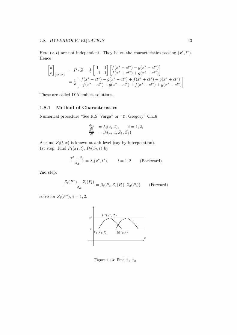
1.8.1 Method of Characteristics
Numerical procedure “See R.S. Varga” or “Y. Gregory” Ch16
dxidt = λi(xi, t), i = 1, 2,dZidt = βi(xi, t, Z1, Z2)
Assume Zi(t, x) is known at t-th level (say by interpolation).
1st step: Find P1(x1, t), P2(x2, t) by
x∗ − xi∆t
= λi(x∗, t∗), i = 1, 2 (Backward)
2nd step:
Zi(P∗)− Zi(Pi)
∆t= βi(Pi, Z1(Pi), Z2(Pi)) (Forward)
solve for Zi(P∗), i = 1, 2.
x
t
P ∗(x∗, t∗)
P1(x1, t) P2(x2, t)t
t∗
Figure 1.13: Find x1, x2
44 CHAPTER 1. FINITE DIFFERENCE METHOD
1.8.2 FDM for Hyperbolic equations
Given pure initial value problem
uxx = utt, u(x, 0) = f(x), ut(x, 0) = g(x).
For j = 0, 1, · · ·
Ui,j−1 − 2Ui,j + Ui,j+1
∆t2=
Ui−1,j − 2Ui,j + Ui+1,j
∆x2i = 1, . . . , N − 1.
Ui,j+1 = m2(Ui−1,j + Ui+1,j) + 2(1−m2)Ui,j − Ui,j−1, m =k
h=
∆t
∆x(1.45)
I.C. First condition is easy to implement, Ui,0 = f(xi). For second condition, use
g(xi) = ut|t=0 =Ui,1 − Ui,−1
2∆t+O(k2) (1.46)
ThusUi,1 − Ui,−1 = 2kgi. (1.47)
For j = 0Ui,1 = m2(Ui−1,0 + Ui+1,0) + 2(1 −m2)Ui,0 − Ui,−1.
Replacing Ui,−1 = Ui,1 − 2kgi, we have
Ui,1 =1
2m2(fi−1 + fi+1) + (1−m2)fi + kgi. (1.48)
Discussion of convergence
We first consider stability. From the consideration of characteristics, we have toassume |m| ≤ 1.(Slope of char.) Let zi,j = ui,j − Ui,j. Then
zi,j+1 = m2(zi−1,j + zi+1,j) + 2(1−m2)zi,j − zi,j−1 +O(k4) +O(k2h2). (1.49)
If we use (1.46) in the first time step,
zi,1 = O(k3). (1.50)
To investigate stability, we try to see thew effect of a single term exp(√−1βx).
I.C becomeszi,0 = exp(
√−1βih). (1.51)
Attempt a solution by separation of variables
zi,j = exp(αjk) exp(√−1βih). (1.52)
1.8. HYPERBOLIC EQUATION 45
Substituting into (1.49) and dropping the truncation error,
eαk + e−αk = 2− 4m2 sin2(1
2βh)
which is
(eαk)2 − 2(1 − 2m2 sin2(1
2βh))eαk + 1 = 0. (1.53)
To avoid increasing solution as j → ∞, it is necessary that |eαk| ≤ 1 for allreal β. But the product of two solution of the quadratic equation is 1, hence oneof the solution must exceed 1 unless both are equal to 1 in magnitude. Thusdiscriminant must be less than 0,
(1− 2m2 sin2(1
2βh))2 ≤ 1.
m2 ≤ 1
sin2(12βh)
This is always true ifm = ∆t/∆x ≤ 1. (1.54)
A more careful analysis shows(Assume m = 1)
‖zj‖ ≤ jBh3 +1
2j(j − 1)Ah4, (1.55)
where ‖zj‖ = maxi |zi,j |. Since t = jh
‖zj‖ ≤ tBh2 +1
2t2Ah2. (1.56)
where
1.8.3 Implicit method for second order hyperbolic equations
Use average of two second central differences:
Ui,j+1 − 2Ui,j + Ui,j−1 =12m
2 (Ui+1,j+1 − 2Ui,j+1 + Ui−1,j+1)+ (Ui+1,j−1 − 2Ui,j−1 + Ui−1,j−1
(1.57)
−m2Ui+1,j+1+2(1−m2)Ui,j+1−m2Ui−1,j+1 = 4Ui,j+m2Ui+1,j−1−2(1+m2)Ui,j−1+m2Ui−1,j−1
(1.58)Note that this method is applicable for problems with finite domain only.


![arXiv:math/0701123v1 [math.AP] 4 Jan 2007 · arXiv:math/0701123v1 [math.AP] 4 Jan 2007 DIFFUSION IN FLUID FLOW: ... Moreover, if the above convergence holds, it is uniform for φ0](https://static.fdocument.org/doc/165x107/5b475ad27f8b9a5e5f8c0ee2/arxivmath0701123v1-mathap-4-jan-2007-arxivmath0701123v1-mathap-4-jan.jpg)


![y φy ε ,ε ,σ2 t - UW Faculty Web Server · 2006-05-01 · Since the above result holds for any r∈[0,1],one might expect that the result holds uniformly for r∈ [0,1].In fact,](https://static.fdocument.org/doc/165x107/5e2a3a72e3fe3d09b20c3719/y-y-f2-t-uw-faculty-web-server-2006-05-01-since-the-above-result.jpg)