Nonparametric Tests for the mean of a Non-negative

Population

Weizhen Wang

Department of Mathematics and Statistics

Wright State University

Dayton, OH 45435

Linda H. Zhao

Department of Statistics

University of Pennsylvania

Philadelphia, PA 19104

Abstract

We construct level-α tests for testing the null hypothesis that the mean of a non-negative

population falls below a prespecified nominal value. These tests make no assumption about

the distribution function other than that it be supported on [0,∞). Simple tests are derived

based on either the sample mean or the sample product. The nonparametric likelihood ratio

test is also discussed in this context. We also derive the uniformly most powerful monotone

(UMP) tests for a sample of size no larger than 2.

MSC: 62G10

Keywords: Level-α test; Markov’s inequality; Non-negative random variable; Nonparametric

likelihood ratio test; UMP test.

1

1 Introduction

This article concerns the problem of constructing one-sided level-α tests for the population mean

of a non-negative random variable. Our discussion thus applies to the common problem of testing

the mean survival time based on an uncensored random sample.

Formally, let X1, . . . , Xn denote the random sample from a population with cumulative dis-

tribution F . Assume PF (X < 0) = 0. In this paper we are primarily interested in constructing

nonparametric tests for the one sided hypothesis

H(�)0 : µ(F ) � µ0 (1.1)

H(>)a : µ(F ) > µ0 or µ(F ) does not exist,

where µ(F ) = EF (X). This is the situation one might encounter for example in trying to establish

that the mean survival time with a test treatment exceeds a known baseline value, µ0.

Let us emphasize that our interest throughout is on examining tests that are valid without

any assumptions on F other than the non-negativity assumption PF (X < 0) = 0. Thus we wish

to construct level-α tests. These are tests with critical functions φ, having power πφ(F ) = EF (φ)

satisfying

sup{πφ(F ) : F ∈ H0} � α. (1.2)

We also wish our tests to be informative in the minimal sense that

sup{πφ(F ) : F ∈ Ha} > α. (1.3)

Informative level-α tests exist for the problem (1.1).

The simplest informative tests are based on the statistic X =1

n

n∑i=1

Xi and discussed in the

next section. Other simple tests are based on the product statistic Q =n∏

i=1

Xi. These tests and

some modifications are discussed in Section 3.

An appealing class of tests is those based on the nonparametric likelihood ratio (NPLR). This

class of tests is described and commented in Section 4, and we make a conjecture there as to how

the NPLR can be used to construct level-α tests. Zhao and Wang (2000) contain further details

about NPLR tests and a discussion of a useful family of NPLR tests which are not quite level α.

2

For the special cases of n ≤ 2 it is possible to derive a UMP monotone test for the problem

(1.1). This is done in Section 5. This derivation validates, for n = 2, the conjecture made in

Section 4 about the NPLR test. It also demonstrates that the level-α tests of Sections 2 - 4 can

all be improved when n = 2. We do not believe that a UMP monotone test exists when n � 3,

but we feel that the construction in Section 5 nevertheless provides convincing evidence that the

tests of Sections 2 - 4 can be improved for all values of n � 2. Section 6 includes a discussion and

comparison of the tests derived in earlier sections. It also contains a plot of the rejection regions

of these tests.

There is another important test for this problem that has occasionally been discussed in the

literature. Anderson (1967) and Breth, Maritz and Williams (BMW) (1978) describe a test whose

foundation is the one sided Kolmogorov confidence region. A similar construction for a related

problem appears in Romano and Wolf (1999). The test proposed by BMW is briefly described in

our concluding section 6.

One qualitative conclusion that can be drawn from the results in our paper is that although

tests of (1.1) satisfying (1.2) and (1.3) exist, even the best of them are not very powerful against

F ∈ H(>)a unless F is “very far” from H

(�)0 . We comment in more detail about this in Section

6. We note there that all the tests have type I error dramatically less than α over most of H(�)0 .

Overall, BMW’s test seems generally preferable to the strictly level-α tests developed in our paper

except when n is small.

Apart from their exact level α property none of the tests (including the BMW’s test) are very

appealing in terms of type I error over H(�)0 and power over H

(>)0 . This strongly motivates also

considering tests that have a nonparametric character but do not strictly satisfy (1.2). Such tests

have been considered by various authors. See Owen (1990, 1999), Romano and Wolf (1999), and

Zhao and Wang (2000) for such proposals, and other related references.

It is natural to ask why we do not also consider the two sided problem subject to PF (X < 0) = 0

of testing

H(=)0 : µ(F ) = µ0 (1.4)

H( �=)a : µ(F ) �= µ0, or µ(F ) does not exist

along with testing of (1.1). Bahadur and Savage (1956) among others have already noted that

3

there is no informative level α-test for this problem when F is not constrained to the non-negative

line.

The following proposition directly shows that there is no informative level-α test of

H(=)0 : µ(F ) = µ0

H(<)a : µ(F ) < µ0, or µ(F ) does not exist,

where F is supported on [0,∞). It also can be understood as saying that any test of (1.4) should

really be interpreted only as a test of (1.1), since tests of (1.4) can be informative only on H(>)a .

Thus we consider only tests of (1.1).

Proposition 1.1 For any critical function φ, and F ∗ supported on [0,∞) and having µ(F ∗) < µ0

sup{πφ(F ) : F ∈ H(=)0 , PF (X < 0) = 0} � πφ(F ∗). (1.5)

Consequently, if φ defines a level-α test of H(=)0 then

πφ(F ) � α whenever µ(F ) < µ0. (1.6)

Proof. Define Fγ ∈ H(=)0 by Fγ = (1 − γ)F ∗ + γI

[µ(F ∗)+µ0−µ(F∗)

γ,∞)

. Then µ(Fγ) = (1 − γ)µ +

γ(µ(F ∗) +µ0 − µ(F ∗)

γ) = µ0, as desired. Also πφ(Fγ) → πφ(F ∗) as γ → 0 for any critical function

φ. This yields (1.5). The assertion (1.6) follows logically from (1.5). �

2 Tests based on the sample mean

With no loss of generality we assume throughout the remainder of the paper that µ0 = 1. The

simplest informative level-α test for the one-sided problem (1.1) is given by

φ1/α(X1, . . . , Xn) =

1 if X � 1/α

0 if X < 1/α.(2.1)

This test has level α as a consequence of the elementary Markov inequality. That is, for F ∈ H(�)0

πφ1/α= PF (X � 1/α)

� 1

1/αEF (X) ≤ α. (2.2)

4

This test is also informative in our sense in that

sup {πφ1/α(F ) : F ∈ H(>)

a } = 1 > α. (2.3)

( Of course inf {πφ1/α(F ) : F ∈ H(>)

a } = 0 � α. This is an inevitable nondesirable property of any

reasonable level-α test of (1.1).)

For n = 1 the Markov inequality is sharp in the sense that there is a distribution F having

µ(F ) = 1 for which equality holds in (2.2). For n � 2 the inequality is not sharp. Hoeffding

and Shrikhande (1955), building on Birnbaum, Raymond and Zuckerman (1947) establish that for

c � 2, n � 2 and µ(F ) = 1

PF (X � c) �

1c− 1

4c2if n is even

1c− n2−1

n21

4c2if n is odd.

(2.4)

They also point out the lower bound

sup {PF (X � c) : µ(F ) � 1} � 1 − (1 − 1

nc)n. (2.5)

Samuels (1969) proves the lower bound above is sharp when c � max(4, n − 1). Beginning from

results in Samuels (1969) we give in the following theorem an upper bound of sup {PF (X � c) :

µ(F ) = 1} which is very close to that in (2.5).

Theorem 2.1 Let [c] denote the largest integer less than or equal to c. Let c′ = min{[c] + 1, n}and Λ(n, c) = n mod(c′), where 0 � Λ(n, c) < c′. Then when c � 4 and n � 5

sup {PF (X � c) : µ(F ) = 1} � U(n, c)

def= 1 − (1 − [n/c′]

nc)c′−Λ(1 − [n/c′] + 1

nc)Λ (2.6)

� 1

c.

See the appendix for a proof.

Remark 1: When c � n− 1, U(n, c) = 1− (1− 1

nc)n which is the lower bound given in (2.5).

The result is obtained in Samuels (1969).

Remark 2: When c < n − 1, U(n, c) is most easily interpreted when both c and n/c are

integers. In this case

U(n, c) = 1 − (1 − 1

c(c + 1))c+1 =

1

c− 1

2c2+ O(

1

c3). (2.7)

5

This can be compared to the right side of (2.4). It is evident that when c is a moderate to large

number then (2.7) improves on the bound (2.4), and is close to the best conceivable inequality

since also (1 − 1nc

)n = 1c− 1

2c2+ O( 1

c3).

The bounds (2.6) and (2.4) can be used to define a level-α test which is better than φ1/α. Let

c6 satisfy

U(n, c6) = α. (2.8)

Then φc6 has level α. For an algebraically simpler but slightly inferior test, one can instead use

(2.4) to get that φc4 has level α where c4 solves

α =

1c− 1

4c2if n is even

1c− n2−1

n21

4c2if n is odd.

(2.9)

In particular, if n is even then c4 =1 +

√1 − α

2α.

It is of interest to compare c6, c4 to c5 where

1 − (1 − 1

nc5

)n = α. (2.10)

(According to (2.5) c5 provides the lower bound for all the tests of the form φc which are α level.)

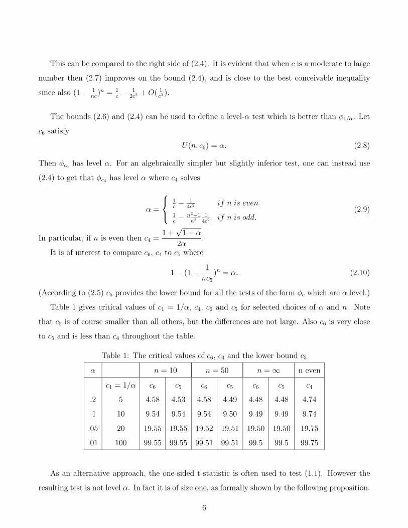
Table 1 gives critical values of c1 = 1/α, c4, c6 and c5 for selected choices of α and n. Note

that c5 is of course smaller than all others, but the differences are not large. Also c6 is very close

to c5 and is less than c4 throughout the table.

Table 1: The critical values of c6, c4 and the lower bound c5

α n = 10 n = 50 n = ∞ n even

c1 = 1/α c6 c5 c6 c5 c6 c5 c4

.2 5 4.58 4.53 4.58 4.49 4.48 4.48 4.74

.1 10 9.54 9.54 9.54 9.50 9.49 9.49 9.74

.05 20 19.55 19.55 19.52 19.51 19.50 19.50 19.75

.01 100 99.55 99.55 99.51 99.51 99.5 99.5 99.75

As an alternative approach, the one-sided t-statistic is often used to test (1.1). However the

resulting test is not level α. In fact it is of size one, as formally shown by the following proposition.

6

For this let S2 =1

n − 1

n∑i=1

(Xi − X)2.

Proposition 2.1 For the problem (1.1), the traditional t-test, which rejects the null hypothesis if

X − 1

S/√

n> tα,n−1 (2.11)

where tα,n−1 is the upper α quantile of Student-t distribution with n − 1 degrees of freedom, has

size one.

Proof. Let Pk be the probability measure on two points 0 and bk = 1 + 1/k with the prob-

abilities, 1 − b−1k and b−1

k , respectively. So the mean of Pk is one and b−nk goes to one as k goes

to infinity. It is clear that the sample point Xk = (bk, . . . , bk)1×n belongs to the rejection region

(2.11) for any k. Therefore the size of the test is at least limk→∞

P ({Xk}) = limk→∞

b−nk = 1. �

3 Tests based on the sample product

Another type of level-α tests of (1.1) is based on the sample product. Consider the critical function

ξc(X1, ..., Xn) =

1 if∏n

i=1 Xi � c

0 otherwise.(3.1)

Theorem 3.1 When c = 1/α, ξc is a size α test. That is, ξ1/α satisfies

sup {πξ1/α(F ) : µ(F ) � 1} = α. (3.2)

Proof. Notice that for a distribution F with µ(F ) � 1,

πξ1/α(F ) = P (

n∏i=1

Xi � 1/α) (3.3)

� αE(n∏

i=1

Xi) = α

n∏i=1

EXi ≤ α.

Also, if we choose

F0 = (1 − α1/n)I[0, ∞) + α1/nI[1/α1/n, ∞), (3.4)

then µ(F0) = 1 and

πξ1/α(F0) = P (

∏Xi � 1/α) = P (Xi = 1/α1/n, i = 1, · · · , n) = α. (3.5)

7

This proves (3.2). �

Because of (3.5) no test of the form ξc with c < 1/α can have level α. So ξc can not be

improved as a level-α test by reducing its critical value, as was the case with φc in the previous

section. However it is possible to describe uniformly more powerful tests than ξ1/α which have

larger rejection regions but still have level α. Here is one such test.

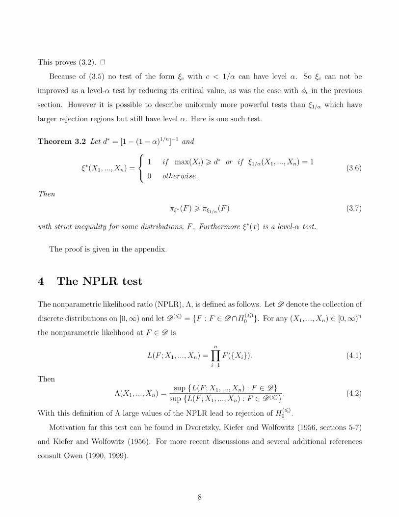
Theorem 3.2 Let d∗ = [1 − (1 − α)1/n]−1 and

ξ∗(X1, ..., Xn) =

1 if max(Xi) � d∗ or if ξ1/α(X1, ..., Xn) = 1

0 otherwise.(3.6)

Then

πξ∗(F ) � πξ1/α(F ) (3.7)

with strict inequality for some distributions, F . Furthermore ξ∗(x) is a level-α test.

The proof is given in the appendix.

4 The NPLR test

The nonparametric likelihood ratio (NPLR), Λ, is defined as follows. Let D denote the collection of

discrete distributions on [0,∞) and let D (�) = {F : F ∈ D∩H(�)0 }. For any (X1, ..., Xn) ∈ [0,∞)n

the nonparametric likelihood at F ∈ D is

L(F ; X1, ..., Xn) =n∏

i=1

F ({Xi}). (4.1)

Then

Λ(X1, ..., Xn) =sup {L(F ; X1, ..., Xn) : F ∈ D}

sup {L(F ; X1, ..., Xn) : F ∈ D (�)} . (4.2)

With this definition of Λ large values of the NPLR lead to rejection of H(�)0 .

Motivation for this test can be found in Dvoretzky, Kiefer and Wolfowitz (1956, sections 5-7)

and Kiefer and Wolfowitz (1956). For more recent discussions and several additional references

consult Owen (1990, 1999).

8

Theorem 4.1 Assume Xi �= Xj for 1 � i < j � n. Then

Λ(X1, ..., Xn) = sup0�ρ�1

n∏i=1

(1 + ρ(Xi − 1)). (4.3)

Note that when ρ = 1n∏

i=1

(1 + ρ(Xi − 1)) =n∏

i=1

Xi.

Hence

Λ(X1, ..., Xn) �n∏

i=1

Xi. (4.4)

It can also be easily checked that equality holds in (4.4) if and only if

n∑i=1

X−1i � n. (4.5)

The proof is deferred to the Appendix.

Consider the test with critical function

η1/α(X1, ..., Xn) = I{Λ(X1,...,Xn)�1/α}. (4.6)

Note that η1/α � ξ1/α because of (4.4), with strict inequality for some (X1, ..., Xn). Hence η1/α is

uniformly more powerful than ξ1/α. We conjecture that η1/α is level α nevertheless - i.e., that

sup{πη1/α(F ) : µ(F ) � 1} = α. (4.7)

When n = 2 one can check that

Λ =

1 if X � 1

X1X2 if X > 1, X−11 + X−1

2 � 2

− (X2−X1)2

4(X2−1)(X1−1)if X > 1, X−1

1 + X−12 > 2.

(4.8)

The results of Section 5 then shows that this conjecture is true (i.e. η1/α is level α) when n = 2

For n � 3 we have not been able to prove or disprove this conjecture. (We have checked that

(4.7) holds for specific choices of n � 3 and for a variety of simple discrete distributions for F .)

Zhao and Wang (2000) investigate a class of tests based on Λ which, however, are not level α over

all of H(�)0 .

9

5 The UMP test for n ≤ 2

In this section, we provide the uniformly most powerful (UMP) tests in certain test classes when

the sample size is less than or equal to two.

5.1 n = 1

When n = 1, the uniformly most powerful nonrandomized test exists. Note that the tests φ1/α in

(2.1), ξ1/α in (3.1), and η1/α in (4.6) coincide. We have the following result.

Theorem 5.1 When n = 1, φ1/α(x) = I{x≥1/α} is the UMP level-α test among all level-α non-

randomized tests.

Proof. Equation (2.2) shows that φ1/α is a level α test. For any nonrandomized level-α test

φ, it suffices to show

φ(x) ≤ φ1/α(x). (5.1)

Suppose the above is not true. Then there is a point x0 < 1/α so that φ(x0) = 1 > 0 = φ1/α(x0).

If x0 < 1, let P0 be a point probability measure on x0. Then P0 ∈ H(�)0 and φ is not a level-α

test because of EP0φ(x) = 1 > α, a contradiction; If x0 ≥ 1, let P0 be a measure having masses

1 − 1/x0 and 1/x0 at zero and x0, respectively. Again, P0 ∈ H(�)0 and EP0φ(x) = 1/x0 > α, a

contradiction. �

There exists a uniformly more powerful test than φ1/α. Let

k1(X) = min(αX, 1).

This function takes all values between 0 and 1, and then defines a randomized test. It is obvious

that k1(x) ≥ φ1/α(x) and the strict inequality holds when x ∈ (0, 1/α). Also

EP (k1(X)) � αEP (X) � α

for any probability P ∈ H(�)0 . Thus k1 is level-α and strictly more powerful than φ1/α whenever

P (0 < X < 1/α) > 0. A natural question is then raised: Does a UMP test among all tests exist?

Here is a negative answer.

10

Proposition 5.1 When n = 1 and 0 < α < 1 there is no UMP level-α test among all level-α

tests.

Proof. Suppose a UMP level-α test k2(X) exists.

First we show that

k2(x) = k1(x)

when x > 1. If this is not true, then there exists a point x0 so that i) k2(x0) > k1(x0) or ii)

k2(x0) < k1(x0). For case i), since k1(x) = 1 when x ≥ 1/α, x0 ∈ (1, 1/α). Let P2 be a measure

having two masses 1 − 1/x0 and 1/x0 at zero and x0, respectively. Then P2 ∈ H(�)0 and

EP2k2(X) ≥ k2(x0)1

x0

> k1(x0)1

x0

= α,

which implies that k2(x) is not level α, a contradiction. For case ii), let P3 be a point probability

at x0. Then P3 ∈ H(>)a and

EP3k2(X) = k2(x0) < k1(x0) = EP3k1(X).

This contradicts the fact that k2(X) is a UMP test.

Secondly, we show that k2(x) = k1(x) on [0,1] as well. For any x0 ∈ [0, 1], consider a probability

P4 having two masses (1 − α)/(1 − x0α) and (α − αx0)/(1 − x0α) at x0 and 1/α, respectively.

It is easy to check that EP4X = 1. Since a UMP test must be a similar test in this problem,

EP4k2(X) = α, which implies

k2(x0) = αx0 = k1(x0).

So far we have proved that the UMP test is equal to k1(x), provided it exists. Consider a

probability P5 having two masses 1 − α/2 and α/2 at zero and 3/α, respectively. P5 ∈ H(>)a .

However,

EP5k1(X) = α/2 < α.

This contradicts with the fact that a UMP test always has a power at least α. Therefore, no UMP

test exists. �

11

5.2 n = 2

When n = 2, for a sample X1, X2 from distribution P on [0,∞), let X(1), X(2) denote the ordered

values of X1, X2. Define P0 = {P on [0,∞) : EP (X) � 1}. Test H0 : P ∈ P0 versus Ha : P ∈{P on [0,∞), P �∈ P0}. Let φ be a test function. We say φ is strongly monotone if φ is a

symmetric function such that x < x′, y < y′ and φ(x, y) > 0 ⇒ φ(x′, y′) = 1; x < x′, y < y′ and

φ(x′, y′) < 1 ⇒ φ(x, y) = 0. We will give the UMP strongly monotone test for n = 2.

Fix α. Let T =1 +

√1 − α

α= (1 −√

1 − α)−1. Define s(t) by

s(t) =

t − √t2 − 1/α if 1√

α� t � 1

α

t − t−1√1−α

if 1α

< t � T .(5.2)

Then for s � t define

φ∗(s, t) = φ∗(t, s) =

1 if t � T

1 if s � s(t), 1√α

� t < T

0 otherwise.

(5.3)

Theorem 5.2 When n = 2, the test φ∗(X1, X2) defined by (5.3) is the UMP strongly monotone

level-α test. In fact if φ is any other strongly monotone level-α test then

φ � φ∗.

The proof is deferred to the Appendix.

6 Discussion

In Sections 2 and 3 we constructed level-α tests of H(�)0 versus H(>)

a . For n = 2 these tests are

strongly monotone and none of these tests is φ∗ defined by (5.3) which is the same to that in (7.24)

. Hence for n = 2 all of the tests defined in Sections 2 and 3 can be improved by the level-α test

φ∗.

It can also be checked that the NPLR test, η1/α, satisfies

ξ1/α(x1, x2) � η1/α(x1, x2) � ξ∗(x1, x2) � φ∗(x1, x2) (6.4)

12

5 10 15 20 25 30 35 40x1

5

10

15

20

25

30

35

40x2

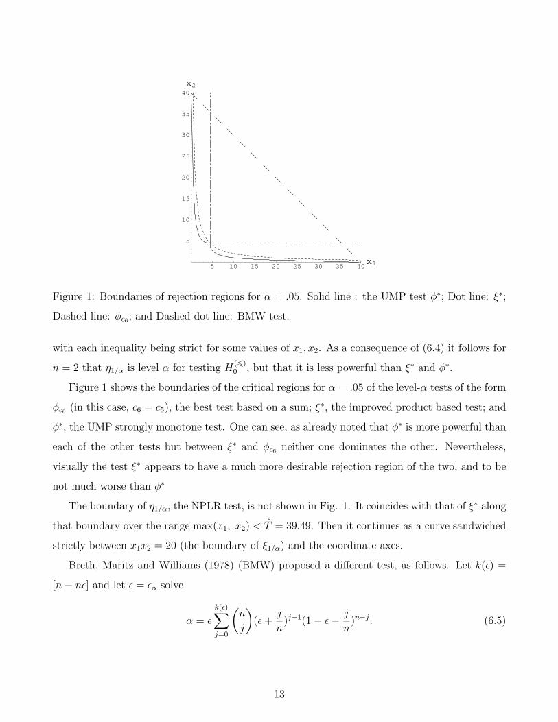
Figure 1: Boundaries of rejection regions for α = .05. Solid line : the UMP test φ∗; Dot line: ξ∗;

Dashed line: φc6 ; and Dashed-dot line: BMW test.

with each inequality being strict for some values of x1, x2. As a consequence of (6.4) it follows for

n = 2 that η1/α is level α for testing H(�)0 , but that it is less powerful than ξ∗ and φ∗.

Figure 1 shows the boundaries of the critical regions for α = .05 of the level-α tests of the form

φc6 (in this case, c6 = c5), the best test based on a sum; ξ∗, the improved product based test; and

φ∗, the UMP strongly monotone test. One can see, as already noted that φ∗ is more powerful than

each of the other tests but between ξ∗ and φc6 neither one dominates the other. Nevertheless,

visually the test ξ∗ appears to have a much more desirable rejection region of the two, and to be

not much worse than φ∗

The boundary of η1/α, the NPLR test, is not shown in Fig. 1. It coincides with that of ξ∗ along

that boundary over the range max(x1, x2) < T = 39.49. Then it continues as a curve sandwiched

strictly between x1x2 = 20 (the boundary of ξ1/α) and the coordinate axes.

Breth, Maritz and Williams (1978) (BMW) proposed a different test, as follows. Let k(ε) =

[n − nε] and let ε = εα solve

α = ε

k(ε)∑j=0

(n

j

)(ε +

j

n)j−1(1 − ε − j

n)n−j. (6.5)

13

Then let X(1) � X(2), . . . � X(n) denote the ordered X1, X2, . . . , Xn and let kα = k(εα) and

H =1

n{

kα∑i=1

X(i) + (n − kα − nεα)X(kα+1)}. (6.6)

Reject H(�)0 when H > 1. H can be most easily described when n − nε is an integer. In this case

take the average of the kα smallest order statistics and n− kα zeros; reject if this average exceeds

1. If [n − nε] < kα < [n − nε] + 1 then a portion of X(kα+1) must be included in this average.

As BMW note it is easy to see that this test has level α. Let Fn denote the sample CDF from

X1, . . . , Xn and let F ∗n,ε(t) = min{Fn(t) + ε, 1}. Then Wilks (1962, p 337) yields

1 − α � PF{F (t) � F ∗n,ε(t) for all t}.

Hence for F ∈ H(�)0

1 − α � PF{1 �∫ ∞

0

tdF (t) =

∫ ∞

0

(1 − F (t))dt ≥∫ ∞

0

(1 − F ∗n,ε(t))dt =

∫ ∞

0

tdF ∗n,ε(t) = H}.

Now we provide further discussions on tests BMW, ξ∗ and φc6 . When n = 2 then εα = 1−√α.

So for α = .05, ε.05 = .776. Consequently for n = 2 the BMW’s test rejects whenever

min(X1, X2) � 1√α

= 4.47. (6.7)

As shown in Figure 1, when n = 2 this test is dominated by ξ∗. Neither of φc6 nor BMW’s test

dominates the other, although BMW’s test might appear more generally desirable.

As n increases BMW’s test quickly appears to be generally the most favorable relative to ξ∗

and φc6 though none of the three tests dominates any other. A brief example can make this clear.

More importantly it also will show that none of the tests has appealing behavior overall, apart

from being level α.

BMW consider the case of Fexp(t) = 1 − e−t ∈ H(�)0 and n = 5 and α = .1. They calculate

that ε = .447 and the type I error of the test at Fexp is

PFexp{H > 1} = .001 < .01.

Both ξ∗ and φc6 have even less type I error at Fexp by several orders of magnitude. On the

other hand consider n = 5, α = .1 and F = G50 =49

50I[0,∞) +

1

50I[50,∞). Then F ∈ H

(�)0 and

14

.1 = PG50{φc6 rejects}, but the other two tests have smaller type I error. Finally if n = 5, α = .1

and F = G101/5 = (1 − 10−1/5)I[0,∞) + 10−1/5I[101/5,∞) ∈ H(�)0 then .1 = PG

101/5{ξ∗ rejects} but

PG101/5

{φc6 rejects} = 0 = P{BMW rejects}.The above pattern is typical for all but very small n. It can for such n be summarized that

for unimodal and similarly well-behaved F ∈ H(�)0 BMW’s test has type I error much less than α

but much larger than ξ∗ or φc6 . On the other hand no test dominates the others, and there are

some very particular distributions in H(�)0 under which either ξ∗ or φc6 has type I error = α, and

is very much better than the other two tests. It should be clear from the fact that the type I error

of these tests is so small on H(�)0 that they have useful power only when F ∈ H

(>)a is rather far

from H(�)0 .

7 Appendix

Proof of Theorem 2.1. Samuels (1969) proves that if Y1, . . . , Ym are independent non-negative

random variables with mean νi and Sm =m∑

i=1

Yi then

P (Sm � mt) � 1 −m∏

i=1

(1 − νi

mt), (7.1)

so long as mt > max[4, (m− 1)]m∑

i=1

νi. The same result for mt = max[4, (m− 1)]m∑

i=1

νi follows by

continuity in {νi}.For c > n− 1 � 4, U(n, c) = 1− (1− 1

nc)n. In this situation Samuels (1969) proves the validity

of (2.6).

For 4 � c � n − 1, define

kj =

j[ nc′ ] if j = 0, 1, . . . , c′ − Λ

j[ nc′ ] + j − (c′ − Λ) if j = c′ − Λ + 1, . . . , c′.

If Λ = 0 then kj = j[n/c′] for j = 0, . . . , c′. In particular, k0 = 0, k1 = [n/c′], and kc′ = n. Also

note that

n = c′[n/c′] + Λ.

15

Define

Yj =

kj∑i=kj−1+1

Xi j = 1, . . . , c′.

Then

E(Yj) =

[n/c′] if j � c′ − Λ

[n/c′] + 1 if c′ − Λ + 1 � j � c′.

Then from (7.1) we have

P (X � c) = P (c′∑

j=1

Yj � nc)

� 1 − (1 − [n/c′]nc

)c′−Λ(1 − [n/c′] + 1

nc)Λ

= U(n, c)

Finally note that U(n, c) < 1/c since (1 − a)b > 1 − ab for 0 < a < 1, b � 2. �.

Proof of Theorem 3.2. Let µ(F ) � 1 and let ρ1 = PF (X1 � d∗). Note that 0 � ρ1 � 1/d∗ =

1 − (1 − α)1/n. Then

πξ∗(F ) = PF (max Xi � d∗) + P (max Xi < d∗)P (∏

Xi � 1/α | max Xi < d∗). (7.2)

Now note that

PF (max Xi � d∗) = 1 − (1 − ρ1)n. (7.3)

Also

E(Xi|Xi < d∗) =

∫ ∞0

xdF (x) − ∫ ∞d∗ xdF (x)

1 − ρ1

� 1 − ρ1d∗

1 − ρ1

, (7.4)

then

P (∏

Xi � 1/α|max Xi < d∗) � (1 − ρ1d

∗

1 − ρ1

)nα. (7.5)

Combining (7.2) − (7.5) yields

πξ∗(F ) � 1 − (1 − ρ1)n + (1 − ρ1)

n(1 − ρ1d

∗

1 − ρ1

)nα

= 1 − (1 − ρ1)n + (1 − ρ1d

∗)nαdef= g(ρ1). (7.6)

Note that ρ1 � 1 − (1 − α)1/n = 1/d∗,

g(0) = α = g(1 − (1 − α)1/n). (7.7)

16

g′(ρ1) = n(1 − ρ1)n−1 − nd∗α(1 − ρ1d

∗)n−1. (7.8)

Hence

g′(0) = n − nd∗α < 0, (7.9)

and

g′(1/d∗) > 0. (7.10)

Finally, g′(ρ) is continuous and has a unique root in (0, 1/d∗). (This root is(d∗α)

1n−1 − 1

(d∗α)1

n−1 d∗ − 1.) It

follows from (7.7) − (7.10) that

g(ρ1) � α (7.11)

(with equality only for ρ1 = 0 and ρ1 = 1/d∗). Refer this fact to (7.6) to see that πξ∗(F ) � α

whenever µ(F ) � 1. �

Proof of Theorem 4.1. It is trivial that the supremum in the numerator of (4.2) occurs

when F = F1, where F1({Xi}) = 1/n, i = 1, . . . , n. It is also easy to see that the supremum in the

denominator of (4.2) must occur at some F for which F ({Xi}) > 0, i = 1, . . . , n, and F ({t}) = 0

unless t = 0 or t = Xi for some i = 1, . . . , n. Hence, let ai = F ({Xi}), i = 1, . . . , n. If min(Xi) > 0

then let a0 = F ({0}); otherwise set a0 = 0. Note that

ai ≥ 0,n∑

i=0

ai = 1 (7.12)

∑aiXi ≤ 1 (7.13)

The supremum in the denominator of (4.2) can then be rewritten

sup{L(F ; X1, . . . , Xn) : F ∈ D (�)} = sup{n∏

i=1

ai} (7.14)

where {ai} satisfies (7.12) and (7.13).

If X � 1 then F1 ∈ D (�) and Λ = 1. Otherwise, let

l(ρ) = logn∏

i=1

(1 + ρ(Xi − 1)). (7.15)

Note that l is strictly concave on [0, 1) (and l(ρ) is continuous and finite at ρ = 1 if and only if

min(Xi) > 0. Further,

l′(0) � 0 if X � 1. (7.16)

17

Hence the right side of (4.3) is 1 when X � 1, as desired.

By the method of Lagrange multipliers, if X > 1 then the supremum on the right of (7.14) is

attained when equality holds in (7.13) and

(n∏

j=1

aj)/ai = (λ1 + λ2Xi) ∀1 � i � n. (7.17)

After some manipulation this can be rewritten as

ai =λ

1 + ρ(Xi − 1), i = 1, . . . , n (7.18)

where λ, ρ are chosen so that (7.12) and (7.13), with equality, are satisfied. Now consider the two

possible cases:

Case 1:∑

X−1i > n. Then we will find a solution to the Lagrange multiplier problem having

a0 = 0. Note that∑

(Xi − 1)ai = 0 implies

l′(ρ) =n∑

i=1

Xi − 1

1 + ρ(Xi − 1)= 0. (7.19)

This equation has a unique positive solution in (0, 1) since

d

dρ(

n∑i=1

Xi − 1

1 + ρ(Xi − 1)) < 0 ,

n∑i=1

(Xi − 1) = n(X − 1) > 0 and

n∑i=1

Xi − 1

Xi

= n −n∑

i=1

Xi < 0.

Let ρ∗ denote this solution. Now note that

∑ 1

1 + ρ∗(Xi − 1)=

∑(

1

1 + ρ∗(Xi − 1)+ ρ∗ Xi − 1

1 + ρ∗(Xi − 1)) = n (7.20)

Hence the choice ρ = ρ∗ and λ = 1/n in (7.18) yields the desired supremum. (It is now easy to

check that the value a0 = 0 does in fact correspond to the desired supremum.) Hence (4.3) holds.

Case 2:∑

X−1i � n. In this case min(Xi) > 0. We find the supremum of

n∏i=1

ai subject to

ai � 0, and (7.13), with equality. This supremum occurs when

(n∏

j=1

aj)/ai = λ2Xi ∀1 � i � n. (7.21)

Since (7.13) holds with equality we have in this case

ai =1/n

Xi

(7.22)

18

and, of course, a0 = 1 − n−1

n∑i=1

X−1i � 0. Since

n∑i=1

ai � 1 in (7.22) it is clear that this solution

also yields the supremum subject to (7.12) and (7.13). Hence Λ =n∏

i=1

Xi. Furthermore, in this

case the supremum on the right of (4.3) is easily seen to be attained when ρ = 1, and hence (4.3)

again holds, as claimed. �

Proof of Theorem 5.2.

The following lemma and its corollary motivate the definition of φ∗ and are a key part of the

proof of the UMP property of φ∗. For convenience in the statement of the lemma define for s � t

ρ(t, s) = ρ(s, t) =

1 if t � 1

1s(2t−s)

if t > 1, s � t −√t2 − t

1 − (t−1)2

(t−s)2if t > 1, s < t −√

t2 − t.

(7.23)

An algebraic calculation shows that φ∗ as defined by (5.3) satisfies

φ∗(s, t) =

1 if ρ(s, t) � α

0 if ρ(s, t) > α.(7.24)

Lemma 7.1 For any 0 � s � t with t > 1 let P(s, t) denote the collection of probability distri-

butions supported on the set {0, s, t} and having mean � 1. Then

sup P∈P(s,t)P (X(1) � s,X(2) � t) = ρ(s, t). (7.25)

This supremum occurs for the distribution P ∗s,t = P ∗ given by (7.26) − (7.30) below:

When

0 � s < t −√

t2 − t (⇒ s < 1) (7.26)

then

P ∗(s) =t − 1

t − s, P ∗(t) =

1 − s

t − s, and P ∗(0) = 0 if s �= 0. (7.27)

When

t � s � t −√

t2 − t (⇒ s >1

2) (7.28)

then

P ∗(s) =t − s

s(2t − s), P ∗(t) =

1

2t − s, (7.29)

19

P ∗(0) =s(t − s) − t(1 − s)

s(2t − s)= 1 − t

s(2t − s)� 0. (7.30)

(Note that (7.28) entails s(2t − s) � t.)

Proof. For any distribution P ∈ P(s, t) let ps = P ({s}), pt = P ({t}). Then ps, pt � 0

ps + pt � 1 (7.31)

and

sps + tpt � 1. (7.32)

Conversely, if ps, pt � 0 satisfying (7.31) and (7.32) then there is a corresponding P ∈ P(s, t)

having P (0) = 1 − ps − pt. Hence it suffices to consider the problem of maximizing

P (X(1) � s,X(2) � t) = 2pspt + p2t (7.33)

subject to (7.31), (7.32) and ps, pt � 0.

When t > 1 the maximum can occur either when both (7.31) and (7.32) are equalities or when

only (7.32) is an equality. (It is easy to check that when t > 1 the maximum cannot occur when

(7.32) is an inequality.) The first case directly yields (7.27) to get ps = (1 − tpt)/s, substitute

this into the objective function 2pspt + p2t , and then maximize over pt. The values at which the

maximum occurs are given by (7.29) and these satisfy (7.31) whenever P ∗(0) given by (7.30)

satisfies p∗(0) > 0. Finally, if p∗(0) > 0 substitute (7.27) into the objective function and (7.29)

into that function and compare the resulting values. The larger of these two values is ρ as given by

(7.23). (The conditions (7.26) and (7.28) describe the regions where (7.27) and (7.29), respectively,

maximize the objective function.) �

This is a standard problem of maximization under inequality constraints. The maximum occurs

when (7.31) and (7.32) are satisfied and

2ps + 2pt = λ1 + tλ2 (7.34)

2pt = λ1 + sλ2. (7.35)

Here, λ2 =2ps

t − s> 0 and equality holds in (7.32). Also λ1 �= 0 only if ps + pt = 1. In that case

λ1 = 2s2 − 2st + t

(t − s)2� 0. Overall, the solution to these Lagrange multiplier equations is given by

(7.26) − (7.30), and yields (7.25) as the maximizing value of R(ps, pt). �

20

Corollary 7.1 If φ is a strongly monotone level-α test of H0 versus Ha then

φ � φ∗. (7.36)

Proof. Suppose (7.36) does not hold. Then there is some 0 � s′ � t′ such that

φ(s′, t′) > 0, φ∗(s′, t′) = 0. (7.37)

It follows from this, strong monotonicity, and the upper semicontinuity of φ∗ that there is some

0 � s � t for which

φ(s, t) = 1, φ∗(s, t) = 0. (7.38)

Note that (7.38) also implies 1 = φ(t, s) = φ(t, t). It then follows from the lemma and property

(7.24) of φ∗ that

sup P∈P(s,t)EP (φ(X1, X2)) � ρ(s, t) > α. (7.39)

Hence φ is not of level α. �

The following two technical lemmas are used in the proof of the main theorem. For 0 � a0 �. . . ,� ak let

P(a0, . . . , ak) = {P ∈ P0 : P supported on {a0, . . . , ak}}. (7.40)

For P supported on {a0, . . . , ak} let pi = P ({ai}), i = 0, . . . , k, so that EP (X) =k∑

i=0

aipi.

Lemma 7.2 Assume 1√α

� ak � 1+√

1−αα

= T , Let a0 = 0, a1 = s(ak). Then

sup P∈P(a0,...,ak){P ∗(ak)k∑

i=1

pi + P ∗(a1)pk} = α, (7.41)

and the supremum is uniquely obtained when p1 = P ∗(a1), pk = P ∗(ak), p(0) = P ∗(0) with

P ∗ = P ∗a1,ak

as in (7.26) − (7.29).

Proof. As in the proof of Lemma 7.1, the maximizing P ∈ P(a0, . . . , ak) must satisfy

P ∗(a1) + P ∗(ak) = λ1 + λ2ak (7.42)

and

P ∗(ak) = λ1 + λ2aj (7.43)

21

for every j = 1, . . . , k − 1 such that pj �= 0. Also, pj = 0, j = 1, . . . , k − 1 only for those

indices, j, for which the left side of (7.43) is smaller than the right side. (Also, λ1 = 0 unless

p0 = 0.) It follows that the unique solution to (7.42), (7.43) maximizing (7.41) has λ1, λ2 as

following (7.34), (7.35), with s = a1, t = ak, and P = P ∗s,t. �

Lemma 7.3 Both 0 < s(t) < 1 and P ∗s,t(0) > 0 if and only if

1 + α−1

2< t < α−1. (7.44)

Let t satisfy (7.44) and s = s(t). Let P ∈ P0(s, t). Then

(P ∗(t) − P (t))P (s) − P ∗(0)P (t) = (1

2t − s− 1 − s

t − s)(

t − 1

t − s) − (

2st − s2 − t

s(2t − s)) (

1 − s

t − s)

> 0 (7.45)

Proof. From (5.2), s(1 + α−1

2) = 1. Hence s(t) < 1 if and only if t >

1 + α−1

2. Also Ps,t(0) > 0

only when t < 1/α, This verifies the assertion at (7.44).

P0(s, t) �= φ since s < 1. In fact, then P0(s, t) contains only the distribution, P , having

p1 = P (s) =t − 1

t − s, p2 =

1 − s

t − s. (7.46)

It is then possible to directly verify the inequality in (7.45) , however the following indirect proof

may be more informative.

Let Qε = (1 − ε)P + εP ∗s,t ∈ P0(0, s, t). It can be checked directly from (5.2) that

p2 < P ∗(t), p1 > P ∗(s). (7.47)

Hence Qε is a distribution whenever

0 � ε � p1/(p1 − P ∗(s)). (7.48)

Now by Lemma 7.1

g(ε) = 2Qε(s)Qε(t) + Q2ε(t) (7.49)

is uniquely maximized at ε = 1. Furthermore, g(ε) is a quadratic in ε, and ε = 1 is in the interior

of its range of definition (since p1/(p1 − P ∗(s)) > 1). Hence g′(0) > 0. Thus

0 < g′(0) = 2p2(P∗(s) − p1) + 2p1(p

∗(t) − p2) + 2p2(P∗(t) − p2)

= 2{p2(P∗(s) + P ∗(t) − p1 − p2) + p1(P

∗(t) − p2)}= 2{−p2P

∗(0) + p1(P∗(t) − p2)}. (7.50)

22

This verifies (7.45). �

Proof of the Theorem. In view of Corollary 7.1 it remains only to show that φ∗ has level α.

So, fix α, 0 < α < 1. For this purpose it then suffices to show that for any finite set A = {a0, . . . , ak}

supP∈P0(A)

EP (φ∗(X1, X2)) � α. (7.51)

There is no loss of generality in assuming that 1/√

α ∈ A (and hence ak � 1/√

α), T ∈ A, and

that for 0 < a < 1/√

α, a ∈ A if and only if s−1(a) ∈ A. For any fixed set, A, of this form the

supremum in (7.51) is attained. Let P ∈ P0(A) be a distribution which attains this supremum.

We will show that P = P ∗s,t for some t and s = sα(t).

We can write A = {a0, a1, . . . , al, 1/√

α, am−l, . . . , am−1, am, am+1, . . . , ak} where a0 = 0, al+1 =

1/√

α, am = T , ai = s(am−i) for i = 1, . . . , l, and ai > T for i = m+1, . . . , k. (Note that m = 2l+2

by virtue of the definition of A.)

Let

λ = min{i : i � 1, pi > 0}, ξ = max{i : pi > 0}. (7.52)

We now proceed to show

ξ � m (7.53)

ξ = m ⇒ p0 > 0 (7.54)

l + 1 � ξ < m ⇔ λ = m − ξ. (7.55)

(Hence, ξ = l + 1 ⇔ λ = l + 1.)

Suppose first that ξ > m, or ξ = m and p0 = 0 , or ξ � l + 2 and 0 < m − ξ < λ. Then for

some ε > 0 define a new distribution P ∈ P0(A) by

pξ = pξ − ε

pξ−1 = pξ−1 + εaξ − aλ

aξ−1 − aλ

(7.56)

pλ = pλ − εaξ − aξ−1

aξ−1 − aλ

where λ = 0 if p0 > 0 and λ = λ otherwise. Also, let pi = pi for i �= λ, ξ − 1, ξ.

Since both pξ > 0 and pλ > 0, one can choose ε > 0 so that all pi � 0. It is then easy

to check that P ∈ P0(A). Furthermore φ∗(aξ, ai) = φ∗(aξ−1, ai) for all i having pi > 0 and

23

φ∗(aλ, ai) � φ∗(aξ−1, ai) with strict inequality for i = λ. It follows that

Ep(φ∗(X1, X2)) > Ep(φ

∗(X1, X2)) (7.57)

This contradicts the assumption that P maximizes (7.51). Hence ξ � m and pm−ξ > 0.

Similarly, if pi = 0 for i � m and pm−λ = 0 then define

pλ = 0

pλ−1 = pλ−1 + pλam − aλ

am − aλ−1

(7.58)

pm = pλaλ − aλ−1

am − aλ−1

.

Then, P ∈ P0(A) and (7.57) holds since φ∗(aλ−1, i) = φ∗(aλ, i) for all i having pi > 0, and

φ∗(aλ−1, am) = 1 with pm > 0 but pm = 0. Again, this contradicts the assumption that p

maximizes (7.51).

The assertions following (7.56) and (7.58) combine to yield (7.53) to (7.55).

Now assume p0 > 0 and either ξ = m or l � λ = m − ξ � 1. Let P ∗ = P ∗aλ,aξ

and

Pε = (1 − ε)P + εP ∗

g(ε) = EPε(φ∗(X1, X2)). (7.59)

Suppose (7.51) is false - i.e., suppose EP (φ∗(X1, X2)) > α, Then

g′(0) = −2α + 2{P ∗(aξ)

ξ∑i=λ

pi + P ∗(aλ)pξ} < 0 (7.60)

by Lemma 7.2 unless P = P ∗. Since there exist values ε < 0 such that Pε ∈ P0(A) it follows that

either P = P ∗ and hence (7.51) holds, or P does not yield the supremum in (7.51), a contradiction.

If p0 > 0 and λ = l + 1 = ξ then P is concentrated on only the two points a0, al+1 = 1/√

α. In

this case P ∗ is also concentrated on just those two points. Hence, again, (7.51) holds.

Finally, if p0 = 0 and l � λ = m − ξ � 1 then aλ = min{supp P}. Hence aλ < 1 since

aξ > 1, pξ > 0 and EP (X) = 1.

There are two possibilities, either P ∗(0) = 0 or P ∗(0) > 0. In the former case the reasoning

involving (7.60) yields that (7.51) holds. If, instead, P ∗(0) > 0 then we apply Lemma 7.3. First

define Q ∈ P0 by

Q({aξ}) = 1 − Q({aλ}) =1 − aλ

aξ − aλ

. (7.61)

24

Then let

Pε = P + ε(P ∗ − Q)

g(ε) = EPε(φ∗(X1, X2)). (7.62)

Note that Pε ∈ P0 for ε � 0 sufficiently small and that pξ � qξ since EP (X) = 1 = EQ(X) and

suppP ⊂ [aλ, aξ]. Then

g′(0+) = 2{(p∗ξ − qξ) + (p∗λ − qλ)pξ}� 2{(p∗ξ − qξ)(qλ + qξ) + (p∗λ − qλ)qξ} (7.63)

(since pξ � qξ and p∗λ − qλ < 0, and qξ + qλ = 1)

= 2{(pξ − qξ)qλ − p∗0qξ} > 0,

by Lemma 7.3. It follows that P is again not the supremum in (7.51), a contradiction.

It follows from the above arguments that P satisfies (7.53)−(7.55). It also follows that P = P ∗,

for otherwise strict inequality holds in (7.60) or (7.63) (whichever is appropriate). But then (7.51)

holds since EP ∗aξ

(φ∗(X1, X2)) = α. This completes the proof of the theorem. �

References

[1] Anderson, T., 1967. Confidence limits for the expected value of an arbitrary bounded random

variable with a continuous distribution function. Bull. ISI, 43, 249-251.

[2] Bahadur, R.R. and Savage, L.J., 1956. The nonexistence of certain statistical procedures in

nonparametric problems. Ann. Math. Statist. 27, 1115-1122.

[3] Breth, M., Maritz, J.S. and Williams, E.J., 1978. On distribution-free lower confidence limits

for the mean of a nonnegative random variable. Biometrika, 65, 529-534.

[4] Birnbaum, Z. W., Raymond, J., and Zuckerman, H.S., 1947. A generalization of Chebyshev’s

inequality to two dimensions. Ann. Math. Statist. 18, 70-79.

[5] Dvoretzky, A., Kiefer, J. and Wolfowitz, J., 1956. Asymptotic minimax character of the

sample distribution function and of the classical multinomial estimator. Ann. Math. Statist.

27, 642-669.

25

[6] Hoeffding, W. and Shrikhande, S.S., 1955. Bounds for the distribution function of a sum of

independent, identically distributed random variables. Ann. Math. Statist. 26, 439-449.

[7] Kiefer, J. and Wolfowitz, J., 1956. Consistency of the maximum likelihood estimator in the

presence of infinitely many incidental parameters. Ann. Math. Statist. 27, 887-906.

[8] Owen, A., 1990. Empirical likelihood ratio confidence regions. Ann, Statist. 18, 90-120.

[9] Owen, A., 1999. Empirical likelihood. Preprint, Stanford University.

[10] Romano, J. P. and Wolf, M., 1999. Finite sample nonparametric inference and large sample

efficiency. Technical report. Stanford University.

[11] Samuels, S. M., 1969. The Markov inequality for sums of independent random variables. Ann.

Math. Statist. 40, 1980-1984.

[12] Wilks, S.S., 1962. Mathematical Statistics. New York, Wiley.

[13] Zhao, L. and Wang, W., 2000. One sided nonparametric likelihood ratio tests for the mean

of non-negative variables. Manuscript in preparation.

26