Nonlinear Four Wave Interactions and Freak Waves Four Wave Interactions and Freak Waves small, and...
37
366 Nonlinear Four Wave Interactions and Freak Waves Peter A.E.M. Janssen Research Department 1 May 2002
Transcript of Nonlinear Four Wave Interactions and Freak Waves Four Wave Interactions and Freak Waves small, and...

366
Nonlinear Four WaveInteractions and Freak Waves
Peter A.E.M. Janssen
Research Department
1 May 2002
For additional copies please contact
The LibraryECMWFShinfield ParkReadingRG2 [email protected]
Series: ECMWF Technical Memoranda
A full list of ECMWF Publications can be found on our web site under:http://www.ecmwf.int/publications/
c©Copyright 2002
European Centre for Medium Range Weather ForecastsShinfield Park, Reading, RG2 9AX, England
Literary and scientific copyrights belong to ECMWF and are reserved in all countries. This publicationis not to be reprinted or translated in whole or in part without the written permission of the Director.Appropriate non-commercial use will normally be granted under the condition that reference is madeto ECMWF.
The information within this publication is given in good faith and considered to be true, but ECMWFaccepts no liability for error, omission and for loss or damage arising from its use.
Nonlinear Four Wave Interactions and Freak Waves
Abstract
Four-wave interactions are shown to play an important role in the evolution of the spectrum of surface gravitywaves. This follows from direct simulations of an ensemble of ocean waves using the Zakharov equation.The theory of homogeneous four-wave interactions, extended to include effects of nonresonant transfer,compares favourably with the ensemble averaged results of the Monte Carlo simulations. In particular,there is good agreement regarding spectral shape. Also, the kurtosis of the surface elevation probabilitydistribution is well-determined by theory even for waves with a narrow spectrum and large steepness. Theseextreme conditions are favourable for the occurence of freak waves.
Technical Memorandum No. 366 1
Nonlinear Four Wave Interactions and Freak Waves
1 Introduction
Presently, there is a considerable interest in understanding the occurrence of freak waves. The notion of freakwaves was first introduced by Draper (1965), and this term is applied for single waves that are extremelyunlikely as judged by the Rayleigh distribution of wave heights (Dean, 1990). In practice, a wave with waveheightH (defined as the distance from crest to trough) exceeding the significant wave heightHS by a factor 2.2 isconsidered to be a freak wave. It is difficult to collect hard evidence on such extreme wave phenomena becausethey occur so rarely. Nevertheless, observational evidence from time series collected over the past decadedoes suggest that for large surface elevations the probability distribution for the surface elevation deviatessubstantially from the one that follows from linear theory with random phase, namely the Gaussian distribution(cf. e.g. Wolfram and Linfoot, 2000).
There are a number of reasons why freak wave phenomena may occur. Often, extreme wave events can beexplained by the presence of ocean currents or bottom topography that may cause wave energy to focus in asmall area due to refraction, reflection and wave trapping. These mechanisms are well understood and may beexplained by linear wave theory (cf. e.g. Lavrenov, 1998).
Trulsen and Dysthe (1997) argue, however, that it is not well understood why exceptionally large waves mayoccur in the open ocean away from non-uniform currents or bathymetry. As an example they discuss the case ofan extreme wave event that happened on January 1, 1995 in the Norwegian sector of the North Sea. Their basicpremise is that these waves can be produced by nonlinear self modulation of a slowly varying wave train. Anexample of nonlinear modulation or focussing is the instability of a uniform narrow-band wave train to side-band perturbations. This instability, known as the side-band, modulational or Benjamin-Feir (1967) instability,will result in focusing of wave energy in space and/or time as is illustrated by the experiments of Lake et al(1977).
To a first approximation the evolution in time of the envelope of a narrow-band wave train is described by thenonlinear Schrodinger equation. This equation, which occurs in many branches of physics, was first discussedin the general context of nonlinear dispersive waves by Benney and Newell (1967). For water waves it was firstderived by Zakharov (1968) using a spectral method and by Hasimoto and Ono (1972) and Davey (1972) usingmultiple-scale methods. The nonlinear Schrodinger equation in one-space dimension may be solved by meansof the inverse scattering transform. For vanishing boundary conditions Zakharov and Shabat (1972) found thatfor large times the solution consists of a combination of envelope solitons and radiation modes, in analogywith the solution of the Korteweg-de Vries equation. However, for two-dimensional propagation, Zakharovand Rubenchik (1974) discovered that envelope solitons are unstable to transverse perturbations, while Cohen,Watson and West (1976) found that a random wave field would break up envelope solitons. This meant thatsolitons could not be used as building blocks of the nonlinear evolution of gravity waves.
For periodic boundary conditions the solution of the nonlinear Schrodinger equation is more complex. Linearstability analysis of a uniform wave train shows that close side-bands grow exponentially in time in goodqualitative agreement with the experimental results of Benjamin and Feir (1967) and Lake et al (1977). For largetimes there is a considerable energy transfer from the carrier wave to the side-bands. In one-space dimension,if there is only one unstable side-band, Fermi-Pasta-Ulam recurrence occurs (Yuen and Ferguson, 1978) inqualitative agreement with the experiments of Lake et al (1977). In the presence of many unstable side-bands,the evolution of a narrow band wave train becomes much more complex. No recurrence is then found (Caponiet al, 1982) and these authors have termed this confined chaos in a nonlinear wave system because most of theenergy resides in the unstable modes. Also, in two-space dimensions (2D) the phenomenon of recurrence is theexception rather than the rule. In addition, in 2D the instability region is unbounded in the perturbation wavevector space, resulting in energy leakage to high wave number modes, hence there is no confined chaos in 2D(Martin and Yuen, 1980). This suggests that the 2D nonlinear Schrodinger equation is inadequate to describe the
2 Technical Memorandum No. 366

Nonlinear Four Wave Interactions and Freak Waves
evolution of weakly nonlinear waves. This was pointed out already by Longuet-Higgins(1978) who performeda stability analysis on the exact equations and found that the instability region is finite in extent. More realisticevolution equations such as the fourth-order evolution equation of Dysthe (1979) or the Zakharov equation(1968) are needed to give an appropriate description of nonlinear gravity waves in two-space dimensions.
Nevertheless, studies of the properties of the nonlinear Schrodinger equation have been vital in understandingthe conditions under which freak waves may occur. This was discussed in detail by Osborne et al (2000). Forperiodic boundary conditions the one-dimensional nonlinear Schrodinger equation may be solved by the inversescattering method as well. The role of the solitons is then replaced by unstable modes. In the linear regime,these modes just describe the evolution in time according to the Benjamin-Feir instability, while by means ofthe inverse scattering transform the fate of the unstable mode may be followed right into the nonlinear regime.Using the inverse scattering transform the solution of the 1D nonlinear Schrodinger equation may be writtenas a ”linear” superposition of stable modes, unstable modes and their mutual nonlinear interactions. Here,the stable modes form a Gaussian background wave field from which the unstable modes occasionally rise upand subsequently disappear again, repeating the process quasi-periodically in time. Making use of the inversescattering transform these authors readily construct a few examples of giant waves from the one-dimensionalnonlinear Schrodinger equation. The question now is what happens in the case of two-dimensional propagation.The notion of solitons is no longer useful, because solitons are unstable in two-dimensions. Osborne et al (2000)show that unstable modes do indeed still exist and that in the nonlinear regime they can take the form of largeamplitude freak waves. Furthermore, the notion of unstable modes seems to be a generic property of deepwater wave trains, as the authors find nonlinear unstable modes in both the one and two-dimensional versionsof Dysthe’s fourth order evolution equation. To summarize this discussion, it seems that freak waves are likelyto occur as long as the wave train is subject to nonlinear focussing. In addition, we only need to study the caseof one-dimensional propagation, because it captures the essentials of the generation of freak waves.
Therefore, in the context of the deterministic approach to wave evolution there seems to be a reasonable the-oretical understanding of why in the open ocean freak waves occur. In ocean wave forecasting practice onefollows, however, a stochastic approach, i.e. one attempts to predict the ensemble average of a spectrum ofrandom waves, because knowledge on the phases is not available. The main problem then is to what extent onecan make statements regarding the occurrence of freak waves in a random wave field. Of course, in the contextof wave forecasting only statements of a probablistic nature can be made. As freak waves imply considerabledeviations from the Normal, Gaussian probability distribution function(pdf) of the surface elevation, the mainquestion therefore is whether we can determine in a reliable manner the pdf of the surface elevation. Since thewave spectrum plays a central role in the stochastic approach the question therefore is whether for given wavespectrum the probability of extreme events may be determined.
Present day wave forecasting systems are based on the energy balance equation (Komen et al, 1994), includinga parametrised version of Hasselmann’s four-wave nonlinear transfer (Hasselmann, 1962). Resonant four-waveinteractions for a random, homogeneous sea play an important role in the evolution of the spectrum of windwaves, because on the one hand they determine the high-frequency part of the spectrum, giving rise to anω−4
tail (Zakharov & Filonenko, 1968), while on the other hand the peak of the spectrum is shifted towards lowerfrequencies. The homogeneous nonlinear interactions give rise to deviations from the Gaussian pdf for thesurface elevation, because the third order nonlinearity generates fourth cumulants of the pdf, while the finitefourth cumulant results in spectral change. An important issue is, however, whether the standard homogeneoustheory can properly describe the generation of freak waves, simply because it does not seem to incorporate theBenjamin-Feir instability mechanism (Alber, 1978, Alber and Saffman, 1978, Crawford et al, 1980, Janssen,1983b). This follows from simple scaling considerations applied to the Hasselmann evolution equation forfour-wave interactions. Since the rate of change of the action densityN is proportional toN3, the nonlineartransfer occurs on the time scaleTNL = O(1/ε4ω0). Here,ε is a typical wave steepness, which is assumed to be
Technical Memorandum No. 366 3
Nonlinear Four Wave Interactions and Freak Waves
small, andω0 is a typical angular frequency of the wave field. In contrast, the Benjamin-Feir instability occurson the much faster timescale ofO(1/ε2ω0).
The Benjamin-Feir instability is an example of a nonresonant four-wave interaction where the carrier wave isphase-locked with the sidebands. This process cannot be described by a theory that assumes that the Fourieramplitudes are not correlated(i.e. a homogeneous wave field), and in which only resonant four-wave interac-tions are considered. For an inhomogeneous, Gaussian narrow-band wave train, Alber and Saffman (1978), andAlber (1978) derived an evolution equation for the Wigner distribution of the sea state. Inhomogeneities gaverise to a much faster energy transfer, comparable with the typical time scale of the modulational instability. Infact, these authors discovered the random version of the Benjamin-Feir instability: a random narrow band wavetrain is unstable to side-band perturbations provided the width of the spectrum is sufficiently narrow. Therefore,one would expect the Alber and Saffman approach to be an ideal starting point for treating freak waves in arandom wave context. However, it is emphasized that this approach has it limitations because deviations fromNormality have not yet been taken into account. In this paper it will be shown, using numerical simulations ofan ensemble of ocean waves, that non-Gaussian effects are quite important while inhomogeneities play only aminor role in the evolution of the ensemble-averaged wave spectrum.
On the other hand, nonresonant interactions appear to be relevant. We extend Hasselmann’s treatment offour-wave interactions by including the effects of nonresonant interactions. As a consequence, the resonancefunction is for short times broader than the usualδ-function and depends on the angular frequency resonanceconditionsand on time. The standard nonlinear transfer is based on the assumption that the action densityspectrum is a slowly varying function of time. It is then argued that the resonance function may be replacedby its large time limit, giving the usual delta function. However, the time span required for the resonancefunction to evolve towards a delta function is so large that considerable changes in the action density functionmay have occurred in the mean time. This will be shown for the special case of one dimensional propagationof surface gravity waves. In those circumstances the standard approach to nonlinear wave-wave interactionswould not give rise to nonlinear transfer, whereas considerable changes of the wave spectrum occur in thenew approach. In fact, there is close agreement between results on the ensemble averaged spectrum and thekurtosis of the pdf of the surface elevation, as obtained from numerical simulations of an ensemble of oceanwaves. Since timeseries from the numerical simulations indicate the occurence of freak waves when the wavesare sufficiently steep (see also Trulsen and Dysthe (1997) or Osborne et al (2000)), the implication is thatan approach to nonlinear transfer, that includes nonresonant interactions seems to capture freak wave events.However, it is strongly emphasized that such an approach can only give statements of a probablistic nature onthe occurrence of extreme wave events.
The structure of this paper is as follows. In Section 2 we review developments regarding the evolution ofa random wave field, but we discuss only the ideas needed for understanding results in the remainder of thispaper. In particular, we extend the standard theory of four wave interactions by including effects of nonresonantinteractions and derive an explicit expression for the kurtosis in terms of the action density spectrum. We alsodiscuss Alber and Saffman’s key result, that according to lowest order inhomogeneous theory there is onlyBenjamin-Feir instability when the wave spectrum is sufficiently narrow. In Section 3 we present results fromMonte Carlo simulations of the nonlinear Schrodinger equation following similar work by Onorato et al (2000).Only one-dimensional wave propagation is discussed. Apart from reasons of economy (we typically do runswith 500 member ensembles), the main reason for this choice is that for one dimension the nonlinear transferaccording to the standard homogeneous theory of four wave interactions vanishes identically. The ensembleaveraged evolution of the wave spectrum clearly shows that there is an irreversible energy transfer resulting in abroadening of the spectrum, while the pdf of the surface elevation has considerable deviations from the Gaussiandistribution. These deviations from Normality may be described, as expected from four-wave interactions, bymeans of the fourth cumulant. In case of nonlinear focussing, the correction to the pdf is such that there
4 Technical Memorandum No. 366
Nonlinear Four Wave Interactions and Freak Waves
is an enhanced probability of extreme events, while in the case of nonlinear defocusing (this was achievedby changing the sign of the nonlinear term) the opposite occurs, namely the probability of extreme events isreduced. This is in agreement with results by Tanaka (1991) who found an increase in groupiness in case ofnonlinear focussing while in the opposite case of a stable wave train groupiness reduces.
Both the spectral broadening and the fourth cumulant (or kurtosis) are found to depend on a single parametercharacterising the narrow-band wave train, namely the ratio of mean square slope to the normalised width ofthe (frequency) spectrum. It is suggested to call this ratio the Benjamin-Feir Index (BFI). If the BFI is largerthan 1 then according to Alber and Saffman (1978) the random wave field is modulationally unstable. Thisresult would suggest that if the BFI is less than 1 no changes in the spectrum occur, while in the opposite casethe unstable side-bands would give rise to a broadening of the wave spectrum. Hence,BFI = 1 is a bifurcationpoint. Our numerical simulations provide no convincing evidence of a bifurcation atBFI = 1. Rather, thereis already a considerable broadening of the wave spectrum aroundBFI = 1, while the dependence of thebroadening on the BFI appears to be smooth rather then abrupt (cf. Tanaka (1991)).
We continue in Section 3 by presenting results from Monte Carlo simulations of the Zakharov equation (Za-kharov, 1968). Results are similar in spirit to thoses obtained with the Nonlinear Schrodinger equation, exceptthat the modulational instability seems to occur for larger BFI. For the nonlinear Schrodinger equation thespectral change owing to nonlinear transfer is symmetrical with respect to the spectral maximum, but this is notthe case for Zakharov equation. In the latter case the nonlinear transfer coefficients and the angular frequencyare asymetrical with respect to the spectral peak and as a consequence there is a down-shift of the peak of thespectrum. It is emphasized that this down-shift occurs in the absence of dissipation, while quantities such asaction, wave momentum and total wave energy are conserved.
In Section 4 an interpretation of the numerical results of Section 3 is given. Firstly, it is shown that inhomo-geneities only play a minor role in the evolution of the wave spectrum, while deviations from Normality aremore relevant. Secondly, results from the numerical solution of the extended version of Hasselmann’s wave-wave interaction approach are presented and compared with the results from Monte-Carlo simulations. A goodagreement is obtained. Apart from the fact that we have given a direct validation of Hasselmann’s four-wavetheory, it also shows that even in extreme conditions such as occur during the generation of freak waves, reliableestimates of deviations from Normality can be made.
In Section 5 a summary of conclusions is given. Much to our surprise, effects of inhomogeneity only play aminor role in understanding the ensemble averaged evolution of surface gravity waves. Homogeneous four-wave interactions, albeit extended by allowing for a time dependent resonance function, seem to capture mostessential features of the averaged nonlinear wave evolution. It seems now possible to estimate the enhancedoccurrence of extreme waves and freak waves on the open ocean since the kurtosis may be estimated directlyfrom the wave spectrum.
2 Review of the theory of a random wave field
Our starting point is the Zakharov equation, which is a deterministic evolution equation for surface gravitywaves in deep water. It is obtained from the Hamiltonian for water waves, first found by Zakharov (1968).Consider the potential flow of an ideal fluid of infinite depth. Coordinates are chosen in such a way that theundisturbed surface of the fluid coincides with thex-y plane. Thez-axis is pointed upward, and the accelerationof gravityg is pointed in the negativez-direction. Letη be the shape of the surface of the fluid, and letφ be thepotential of the flow. Hence, the velocity of the flow follows from~u =−∇φ.
Technical Memorandum No. 366 5
Nonlinear Four Wave Interactions and Freak Waves
By choosing as canonical variables
η, and, ψ(~x, t) = φ(~x,z= η, t), (1)
Zakharov (1968) showed that the total energyE of the fluid may be used as a Hamiltonian. Here,
E =12
∫ ∫ η
−∞dzd~x
((∇φ)2 +(
∂φ∂z
)2)
+g2
∫d~xη2. (2)
The x-integrals extend over the total basin considered. If an infinite basin is considered the resulting totalenergy is infinite, unless the wave motion is localized within a finite region. This problem may be avoided byintroducing the energy per unit area by dividing (2) by the total surfaceL×L, whereL is the length of the basin,and taking the limit ofL→ ∞ afterwards. As a consequence, integrals over wave number~k are replaced bysummations whileδ-functions are replaced by Kroneckerδ’s. For a more complete discussion cf. Komen et al(1994). We will adopt this approach implicitely in the remainder of this paper.
The boundary conditions at the surface, namely the kinematic boundary condition and Bernoulli’s equation, arethen equivalent to Hamilton’s equations,
∂η∂t
=δEδψ
,∂ψ∂t
=−δEδη
, (3)
whereδE/δψ is the functional derivative ofE with respect toψ, etc. Inside the fluid the potentialφ satifiesLaplace’s equation,
∇2φ+∂2φ∂z2 = 0 (4)
with boundary conditionsφ(~x,z= η) = ψ (5)
and∂φ(~x,z)
∂z= 0, z→ ∞. (6)
If one is able to solve the potential problem, thenφ may be expressed in term of the canonical variablesη andψ. Then the energyE may be evaluated in terms of the canonical variables, and the evolution in time ofη andψ follows at once from Hamilton’s equations (Eq.(3)). This was done by Zakharov (1968), who obtained thedeterministic evolution equations for deep water waves by solving the potential problem (4-6)in an iterativefashion for small steepnessε. In addition, the Fourier transforms ofη andφ were introduced, while resultscould be expressed in a concise way by use of the action variableA(~k, t). For example, in terms ofA the surfaceelevationη becomes
η =∫ ∞
−∞d~k
(k
2ω
)1/2
[A(~k)+A∗(−~k)]ei~k.~x. (7)
Here,~k is the wave number vector,k its absolute value, andω =√
gk denotes the dispersion relation of deep-water, gravity waves. Substitution of the series solution forφ into the Hamiltonian(2) gives an expansion of thetotal energyE of the fluid in terms of wave steepness,
E = ε2E2 + ε3E3 + ε4E4 +O(ε5). (8)
Retaining only the second-order term ofE corresponds to the linear theory of surface gravity waves, the third-order term corresponds to three-wave interactions, and the fourth-order term corresponds to four-wave interac-tions. Since resonant three-wave interactions are absent for deep-water gravity waves, a meaningful description
6 Technical Memorandum No. 366
Nonlinear Four Wave Interactions and Freak Waves
of the wave field is only obtained by going to fourth order inε. In fact, Krasitskii (1990) has shown that inthe absence of resonant three wave interactions there is a nonsingular, canonical transformation from the ac-tion variableA to the new variablea that allows elimination of the third order contribution to the wave energy.Loosely speaking, the new variablea descibes the free wave part of the wave field. Apart from a constant factor,the energy of the free waves becomes,
E =∫
d~k1ω1a∗1a1 +12
∫d~k1,2,3,4T1,2,3,4a∗1a∗2a3a4δ1+2−3−4, (9)
wherea1 = a(~k1), etc.,δ is the Dirac delta function and the interaction matrixT is given by Krasitskii (1990).The interaction matrix enjoys a number of symmetry conditions, of which the most important one isT1,2,3,4 =T3,4,1,2 as this condition implies thatE is conserved. Hamilton’s equations now become the single equation
i∂a∂t
=δEδa∗
, (10)
and, evaluating the functional derivative ofE with respect toa∗, the evolution equation fora becomes
∂a1
∂t+ iω1a1 =−i
∫d~k2,3,4T1,2,3,4a∗2a3a4δ1+2−3−4, (11)
known as the Zakharov equation. Apart from the free wave energy (9) the Zakharov equation admits conserva-tion of action and of wave momentum as
a)ddt
∫d~k1a1a∗1 = 0,
b)ddt
∫d~k1~k1a1a∗1 = 0. (12)
2.1 Comments on the Zakharov Equation
The properties of the Zakharov equation have been studied in great detail by, for example, Crawford et al (1981)(for an overview see Yuen and Lake, 1982). Thus the nonlinear dispersion relation, first obtained by Stokes(1947), follows from Eq.(11), while also the instability of a weakly nonlinear, uniform wave train (the so-calledBenjamin-Feir instability) is well described by the Zakharov equation; the results on growth rates, for example,are qualitatively in good agreement with the results of Longuet-Higgins (1978). However, these results wereobtained with a form of the interaction matrixT that did not result in a Hamiltonian form of Eq.(11). Krasitskii(1990) found the correct canonical transformation to eliminate the cubic interactions, which resulted in aT thatsatisfied the appropriate symmetry conditions for Eq.(11) to be Hamiltonian. Krasitskii and Kalmykov (1993)studied the differences between the Hamiltonian and the non-Hamiltonian forms of the Zakharov equation butonly for large amplitude differences in the solution were found.
In this paper we initially use a narrow-band approximation to the Zakharov equation, because the main impactof the Benjamin-Feir instability is found near the spectral peak. This approximate evolution equation is obtainedby means of a Taylor expansion of angular frequencyω and the interaction matrixT around the carrier wavenumber~k0. The nonlinear Schrodinger equation is then obtained by using only the lowest order approximationto T given by k3
0, while angular frequencyω is expanded to second order in the modulation wave number~p =~k−~k0. The main advantage of the use of the nonlinear Schrodinger equation is that many properties ofthis equation are known and that it can be solved numerically in an efficient way. The drawback is, however,that it overestimates the growth rates of the Benjamin-Feir instability and that the nonlinear energy transfer
Technical Memorandum No. 366 7
Nonlinear Four Wave Interactions and Freak Waves
is symmetrical with respect to the carrier wave number. For this reason, we study solutions of the completeZakharov equation as well, using the Krasitskii (1990) expression for the interaction matrixT. Similarly, onecould study higher-order evolution equations such as the one by Dysthe (1979), but we found that spectra maybecome so broad that the narrow-band approximation becomes invalid.
Another reason for studying the nonlinear Schrodinger equation is that it allows us to introduce an importantparameter which will be used to stratify the numerical and theoretical results. From the physical point ofview we are basically studying a problem that concerns the balance between dispersion of the waves and itsnonlinearity. For the full Zakharov equation it will be difficult to introduce a unique measure of, for example,nonlinearity because the nonlinear transfer matrixT is a complicated function of wave number. However, inthe narrow-band approximation, giving the nonlinear Schrodinger equation, this is more straight-forward to do.Balancing the nonlinear term and the dispersive term in the narrow-band version of Eq.(11) therefore gives thedimensionless number
− gT0
ω0
1
k40ω′′0
s2
σ′2ω. (13)
Since our interest is in the dynamics of a continuous spectrum of waves the slope parameters and the relativewidth σ′ω of the frequency spectrum relate to spectral properties, hences = (k2
0 < η2 >)12 , with < η2 > the
average surface elevation variance, andσ′ω = σω/ω0. For positive sign of the dimensionless parameter (13)there is focussing (modulational instability) while in the opposite case there is defocussing of the weakly non-linear wave train. Based on this we introduce the Benjamin-Feir(BF) Index, which, apart from a constant, isthe square root of the dimensionless number (13). Using the dispersion relation for deep-water gravity wavesand the expression for the nonlinear interaction coefficient,T0 = k3
0, the BF Index becomes,
BFI = s√
2/σ′ω. (14)
The BF Index turns out to be very useful in ordering the theoretical and numerical results presented in thefollowing Sections. For simple initial wave spectra that only depend on the variance and on the spectral width,it can be shown that for the nonlinear Schrodinger equation the solution is completely characterized by the BFIndex. For the Zakharov equation this is not the case, but the BF Index is still expected to be a useful parameterfor narrow-band wave trains.
2.2 Stochastic approach
The Zakharov equation (11) predicts amplitude and phase of the waves. For practical applications such as waveprediction, the detailed information regarding the phase of the waves is not available. Therefore, at best onecan hope to predict average quantities such as the second moment
B1,2 =< a1a∗2 >, (15)
where the angle brackets denote an ensemble average. Here, we briefly sketch the derivation of the evolutionequation for the second moment from the Zakharov equation, assuming a zero mean value,< a1 >= 0. It isknown, however, that because of nonlinearity, the evolution of the second moment is determined by the fourthmoment, and so on, resulting in an infinite hierarchy of equations (Davidson, 1972). To obtain a meaningfultruncation of this hierachy, it is customary to assume that the probability distribution fora1 is close to a Gaussiandistribution, an assumption which is a reasonable one for small wave steepnessε. In that event, higher-ordermoments can be expressed in lower-order moments. In general, for a zero-mean stochastic variablea1, onefinds that the fourth moment becomes
< a jaka∗l a∗m > = B j,l Bk,m+B j,mBk,l +D j,k,l ,m, (16)
8 Technical Memorandum No. 366
Nonlinear Four Wave Interactions and Freak Waves
whereD is the so-called fourth cumulant, which vanishes for a Gaussian sea state. Resonant nonlinear interac-tions, however, will tend to create correlations in such a way that a finite fourth cumulant results. But for smallsteepnesD is expected to be small, so that an approximate closure of the infinite hierarchy of equations may beachieved.
Let us now sketch the derivation of the evolution equation for the second moment< aia∗j > from the Za-kharov equation (11). To that end, we multiply Eq.(11) for ai by a∗j , add the complex conjugate withi and jinterchanged, and take the ensemble average:[
∂∂t
+ i(ωi−ω j)]
Bi, j =
− i∫
d~k2,3,4[Ti,2,3,4 < a∗j a∗2a3a4 > δi+2−3−4−c.c.(i ↔ j)], (17)
wherec.c. denotes complex conjugate, andi ↔ j denotes the operation of interchanging indicesi and j inthe previous term. Because of nonlinearity the equation for the second moment involves the fourth moment.Similarly, the equation for the fourth moment involves the sixth moment. It becomes[
∂∂t
+ i(ωi +ω j −ωk−ωl )]
< aia ja∗ka∗l >=
− i∫
d~k2,3,4[Ti,2,3,4 < a∗2a∗ka∗l a3a4a j > δi+2−3−4 +(i ↔ j)]
+ i∫
d~k2,3,4[Tk,2,3,4 < a∗3a∗4a∗l a2aia j > δk+2−3−4 +(k↔ l)]. (18)
So far, no approximations have been made. In the next Section, we discuss the implications of the assumptionsof a homogeneous weakly nonlinear wave field. Homogeneity of the wave field, however, does not allow adescription of the Benjamin-Feir instability, and therefore in the following Section we discuss the consequencesfor spectral evolution when the wave field is allowed to be inhomogeneous.
2.3 Evolution of a homogeneous random wave field
A wave field is considered to be homogeneous if the two point correlation function< η(~x1)η(~x2) > dependsonly on the distance~x1−~x2. Using the expression for the surface elevation, Eq.(7), it is then straightforward toverify that a wave field is homogeneous provided that the second momentBi, j satisfies
Bi, j = Niδ(~ki−~k j), (19)
whereNi is the spectral action density, which is equivalent to a number density becauseωiNi is the spectralenergy density, while~kiNi is the spectral momentum density (apart from a factorρw).
For weakly nonlinear waves the fourth cumulantD is small compared to the product of second-order cumu-lants (this may be verified afterwards, it follows immediately from Eq.(18). Now, invoking the random-phaseapproximation (i.e. Eq.(16)) with D = 0) on Eq.(17), combined with the assumption of a homogeneous wavefield results in constancy of the second momentBi, j . Hence, the need to go to higher order; that is the fourthmoment has to be determined through Eq.(18).
Application of the random phase approximation to the sixth moment and solving Eq.(18) for the fourth cumu-lantD, subject to the initial valueD(t = 0) = 0, gives
Di, j,k,l = 2Ti, j,k,l δi+ j−k−l G(∆ω, t) [NiNj(Nk +Nl )− (Ni +Nj)NkNl ] (20)
Technical Memorandum No. 366 9
Nonlinear Four Wave Interactions and Freak Waves
where∆ω is short hand forωi +ω j −ωk−ωl , and we have made extensive use of the symmetry properties ofthe nonlinear transfer matrixT, in particular the Hamiltonian symmetry. In addition, we used the property that,according to Eq.(17) the action densityN only evolves on the slow time scale. The functionG is defined as
G(∆ω, t) = i∫ t
0dτei∆ω(τ−t) = Rr(∆ω, t)+ iRi(∆ω, t), (21)
where
Rr(∆ω, t) =1−cos(∆ωt)
∆ω, (22)
while
Ri(∆ω, t) =sin(∆ωt)
∆ω. (23)
The functionG develops for large timet into the usual generalised functionsP/∆ω, andδ(∆ω), since,
limt→∞
G(∆ω, t) =P
∆ω+πiδ(∆ω), (24)
a relation which is, strictly speaking, only meaningful inside integrals over wave number when multiplied by asmooth function.
Substitution of Eq.(20) into Eq.(17) eventually results in the following evolution equation for four-wave inter-actions,
∂∂t
N4 = 4∫
d~k1,2,3T21,2,3,4δ(~k1 +~k2−~k3−~k4)Ri(∆ω, t)
× [N1N2(N3 +N4)−N3N4(N1 +N2)] , (25)
where now∆ω = ω1 +ω2−ω3−ω4. This evolution equation is usually called the Boltzmann equation.
Two limits of the resonance functionRi(∆ω, t) are of interest to mention. For small times we have
limt→0
Ri(∆ω, t) = t (26)
while for large times we have
limt→∞
Ri(∆ω, t) = πδ(∆ω). (27)
Hence, according to Eq.(25), for short times the evolution of the action densityN is caused by both resonantand nonresonant four-wave interactions, while for large times, when the resonance functions evolves towards aδ-function, only resonant interactions contribute to spectral change.
In the standard treatment of resonant wave wave interactions (cf., for example Hasselmann (1962) and David-son (1972)) it is argued that the resonance functionRi(∆ω, t) may be replaced by its time-asymptotic value(Eq.(27)), because the action density spectrum is a slowly varying function of time. However, the time requiredfor the resonance function to evolve towards a delta function may be so large that in the mean time consider-able changes in the action density may have occurred. For this reason we will keep the full expression for theresonance function.
An important consequence of this choice concerns the estimation of a typical time scaleTNL for the nonlinearwave-wave interactions in a homogeneous wave field. Withε a typical wave steepness andω0 a typical angular
10 Technical Memorandum No. 366
Nonlinear Four Wave Interactions and Freak Waves
frequency of the wave field, one finds from the Boltzmann equation(25) that for short timesTNL = O(1/ε2ω0),while for large timesTNL = O(1/ε4ω0). Hence, although the standard nonlinear transfer, which uses as reso-nance function Eq.(27), does not capture the physics of the modulational instability (which operates on the fasttime scale 1/ε2ω0), the full resonance function does not suffer from this defect.
It is also important to note that according to the standard theory there is only nonlinear transfer for two-dimensional wave propagation. In the one-dimensional case there is no nonlinear transfer in a homogeneouswave field. The reason for this is that only those waves interact nonlinearly that satisfy the resonance conditions~k1 +~k2 =~k3 +~k4 andω1 + ω2 = ω3 + ω4. In one dimension these resonance conditions can only be met forthe combinations~k1 =~k3,~k2 =~k4 or~k1 =~k4,~k2 =~k3. Then, the rate of change of the action density, as givenby Eqns.(25 and27), vanishes identically because of the symmetry properties of the term involving the actiondensities. This contrasts with the Benjamin-Feir instability which has its largest growth rates for waves in onedimension. On the other hand, using the complete expression for the resonance function, there is always anirreversible nonlinear transfer even in the case of one-dimensional propagation.
The Boltzmann equation, Eq.(25), admits just as the deterministic Zakharov equation, conservation of totalaction, wave momentum, while the ensemble average of the Hamiltonian (Eq.(9)) is conserved as well (Thelast conservation law follows from Eqs.(25) by consistently utilizing the assumption of a slowly varying actiondensity). It is emphasized that the Hamiltonian consists of two parts, the energy according to linear wave theoryand a nonlinear interaction term. Therefore, unlike the standard theory of four-wave interactions, the linearexpression for the wave energy is not conserved. The exception occurs for large times when the resonancefunction Ri has evolved towards aδ-function, and then just as in the standard theory the linear wave energyis conserved. This follows also from the numerical simulations presented in Section 3 which show that theensemble average of the Hamilonian is conserved but, in particular for short times, not the linear wave energy.Furthermore, it should be mentioned that the Boltzmann equation(25) has the time reversal symmetry of theoriginal Zakharov equation, since the resonance function changes sign when timet changes sign. Also, asRi
vanishes fort = 0, the time derivative of the action density spectrum is continuous aroundt = 0 and does notshow a cusp. (cf. Komen et al, 1994). Nevertheless, despite the fact that there is time reversal, Eq.(25) hasthe irreversibility property: the memory of the inital conditions gets lost in the course of time owing to phasemixing.
The standard nonlinear transfer in a homogeneous wave field has been studied extensively in the past fourdecades. The JONSWAP study (Hasselmann et al, 1973) has shown the prominent role played by four-waveinteractions in shaping the wave spectrum, and in shifting the peak of the spectrum towards lower frequencies.Modern wave forecasting systems therefore use a parametrization of the nonlinear transfer (Komen et al, 1994).
Our main interest in this paper is in the statistical aspects of random, weakly nonlinear waves in the context ofthe Zakharov equation. In particular we are interested in the relation between the deviations from the Gaussiandistribution and four-wave interactions. Because of the symmetries of the Zakharov equation, the first momentof interest is then the fourth moment and the related kurtosis. The third moment and its related skewnessvanishes: information on the odd moments can only be obtained by making explicit use of Krasitskii’s (1990)canonical transformation. Now, the fourth moment< η4 > may be obtained in a straightforward manner fromEq.(16) and the expression for the fourth cumulant Eq.(20) as
< η4 >=3
4g2
∫d~k1,2,3,4(ω1ω2ω3ω4)
12 < a1a2a∗3a∗4 > +c.c (28)
Denoting the second moment< η2 > by m0, deviations from Normality are then most conveniently establishedby calculating the kurtosis
C4 =< η4 > /3m20−1,
Technical Memorandum No. 366 11
Nonlinear Four Wave Interactions and Freak Waves
since for a Gaussian pdfC4 vanishes. The result forC4 is
C4 =4
g2m20
∫d~k1,2,3,4T1,2,3,4δ1+2−3−4(ω1ω2ω3ω4)
12 ×Rr(∆ω, t)N1N2N3, (29)
whereRr is defined by Eq.(22). For large times, unlike the evolution of the action density, the kurtosis does notinvolve a Diracδ-function but rather depends onP/∆ω. Therefore, the kurtosis is determined by the resonantand nonresonant interactions. It is instructive to apply Eq.(29) to the case of a narrow band wave spectrum inone dimension. Hence, performing the usual Taylor expansions around the carrier wave numberk0 to lowestsignificant order, one finds for large times
C4 =8ω2
0
g2m20
T0
ω′′0
∫dp1,2,3,4
δ1+2−3−4
p21 + p2
2− p23− p2
4
N1N2N3, (30)
where p = k− k0 is the wave number with respect to the carrier. It is seen that the sign of the kurtosis isdetermined by the ratioT0/ω′′0, which is the same parameter that determines whether a wave train is stable ornot to side-band perturbations. Remark that numerically the integral is found to be negative, at least for bell-shaped spectra. Hence, from Eq.(30) it is immediately plausible that for an unstable wave system which hasnegativeT0/ω′′0 the kurtosis will be positive and thus will result in an increased probability of extreme events.On the other hand for a stable wave system there will a reduction in the probability of extreme events.
Finally, a further simplification of the expression for the kurtosis may be achieved if it is assumed that the wavenumber spectrumF(p) = ω0N(p)/g only depends on two parameters namely, the variancem0 and the spectralwidth σk. Introduce the scaled wave numberx = p/σk and the correspondingly scaled spectrumm0H(x)dx=F(p)dp. Then, using the deep-water dispersion relation andT0 = k3
0, Eq.(30) becomes
C4 =−8
(s
σ′ω
)2
J, (31)
wheres is the significant steepnessk0m120 while σ′ω is the relative width in angular frequency spaceσω/ω0 =
0.5σk/k0. The parameterJ is given by the expression
J =∫
dx1,2,3,4δ1+2−3−4
x21 +x2
2−x23−x2
4
H1H2H3,
and is independent of the spectral parametersm0 andσk. Therefore, Eq.(31) suggests a simple dependence ofthe kurtosis on spectral parameters. In fact, the kurtosis depends on the square of the BF index introduced inEq.(13).
2.4 Evolution of an inhomogeneous random wave field
The Benjamin-Feir instability is the result of a nonlinear interaction of waves that are phase-locked, as thecarrier wave is phase-locked with the sidebands and therefore this process cannot be described by a theorythat assumes that the Fourier amplitudes are not correlated, as expressed by the assumption of homogeneity ofthe wave field (cf. Eq.(19)). Therefore, this suggests that local nonlinear events such as freak waves could bebeyond the scope of the standard description of ocean waves.
The investigation of the effect of inhomogeneities on the nonlinear energy transfer started with the work ofAlber (1978), and Alber and Saffman (1978), while Crawford et al (1980) combined the effects of inhomo-geneity and non-Normality on the evolution of weakly nonlinear water waves. A review of this may be found
12 Technical Memorandum No. 366
Nonlinear Four Wave Interactions and Freak Waves
in Yuen and Lake (1982). We will only discuss the lowest order effects of inhomogeneity, disregarding anyeffects resulting from deviations from Normality, and we only discuss one-dimensional wave propagation.
Hence, we do not impose the condition of a homogeneous wave field (cf. Eq.(19)). Now invoking the Gaussianapproximation on the fourth moment(16 with D = 0) and substituting the result in the evolution equation forthe second moment, Eq.(17), gives[
∂∂t
+ i(ωi−ω j)]
Bi, j =−2i∫
d~k2,3,4[Ti,2,3,4δi+2−3−4B3, jB4,2−Tj,2,3,4δ j+2−3−4Bi,3B2,4] (32)
Here, we used the property that the second momentB is hermitian,Bi, j = B∗j,i , and we made use of the symmetryproperties ofT.
In principle, Eq.(32) could be used to study the (in)stability of a homogeneous wave spectra, but to our knowl-edge this has not been done so far. In stead of this, Alber (1978) and Alber and Saffman (1978) studied thestability of a narrow-band, homogeneous wave spectrum. Following Crawford et al (1980) and Yuen and Lake(1982), a considerable simplification of the evolution equation forBi, j may be achieved by expanding angularfrequencyω and interaction coefficientT around the carrier wave numberk0. At the same time one introducesthe sum and difference wave numbers
n =12(ki +k j),m= ki−k j (33)
while we introduce the relative wave numberp = n−k0. The correlation functionB is from now on regardedas a functionm andn. Realising that in the narrow band approximationn is close tok0 while m is small, oneobtains from Eq.(32) the following approximate evolution equation forB,[
∂∂t
+ im(ω′0 + pω′′0)]
Bn,m =−2iT0
∫dl [Bn− 1
2 l ,m−l −Bn+ 12 l ,m−l ]
∫dkBk,l . (34)
Here, a prime denotes differentation with respect to the carrier wave numberk0, while T0 = k30. A key role in
the work of Alber and Saffman is played by the envelope spectral functionW(p,x, t), which is in fact a Wignerdistribution (Wigner, 1932). It is related to the Fourier transform ofB(n,m, t) with respect tom,
W(p,x, t) =2ω0
g
∫dmeimxB(n,m, t). (35)
and a homogeneous sea state simply has a Wigner distribution which is independent of the spatial coordinatex, in agreement with the definition of homogeneous sea given in Eq.(19). In terms of the Wigner distributionEq.(34) becomes a transport equation inx, p andt, which bears a similarity with the Vlasov Equation fromplasma physics. This transport equation is obtained by means of a Taylor expansion of the difference term inthe right-hand side of (34) with respect tol , giving an infinite sum. The result is[
∂∂t
+(ω′0 + pω′′0)∂∂x
]W =
gT0
ω0
∂ρ∂x
∂W∂p
+ ... , (36)
whereρ(x, t) = 2 < η2 > is the mean square envelope variance, given by
ρ(x, t) =∫
dp W(p,x, t), (37)
while the dots on the right-hand side of Eq.(36) represent the remaining terms of the Taylor series expansion.Note that all terms of the series are required to properly recover the random-version of the Benjamin-Feirinstability.
Technical Memorandum No. 366 13
Nonlinear Four Wave Interactions and Freak Waves
Alber and Saffman (1978) and Alber (1978) studied the stability of a homogeneous spectrum and found thatit is unstable to long wave length perturbations if the width of the spectrum is sufficiently small. In otherwords, in case of instability inhomogeneities would be generated by what we term the random version of theBenjamin-Feir instability, therefore violating the assumption of homogeneity made in the standard theory ofwave-wave interactions.
To see whether a homogeneous spectrumW0(p) is stable or not, one proceeds in the usual fashion by perturbingW0(p) slightly according to
W = W0(p)+W1(p,x, t),W1�W0. (38)
Linearizing the evolution equation forW around the equilibriumW0 and considering normal mode perturbationsone obtains a dispersion relation between the angular frequencyω and the wave numberk of the perturbation.Instability is found forIm(ω) > 0. Alber (1978) considered as special case the Gaussian spectrum
W0(p) =< a2
0 >
σk√
2πexp(− p2
2σ2k
), (39)
where< a20 > is a constant envelope variance andσk is the width of the spectrum in wave number space.
Stability of the random wave train was found when the relative width of the spectrum,σk/k0, exceeds a measureof mean square slope. In terms of the relative widthσω/ω0 of the frequency spectrum, which is just half therelative width for the wave number spectrum, one finds stability if
σω
ω0> (k2
0 < a20 >)
12 , (40)
while in the opposite case there is instability of the random wave train. Note that in terms of the BF Index thestability condition Eq.(40) simply becomesBFI < 1.
As a consequence, one should expect to find in nature spectra with a width larger than the right hand side ofEq.(40), because for smaller width the random version of the Benjamin-Feir instability would occur, resulting ina rapid broadening of the spectral shape. For a random narrow-band wave train this broadening is an irreversibleprocess because of phase mixing (Janssen, 1983b). The broadening of the spectrum is associated with thegeneration of inhomogeneities in the wave field. To appreciate this point, we mention that the evolution equation(36) satisfies a number of conservation laws. Using the already introduced envelope surface elevation varianceρ(x) the first few conservation laws are given by
a)ddt
∫dxρ(x) = 0,
b)ddt
∫dxdp pW= 0, (41)
c)ddt
[ω′′0
∫dxdp p2W+
gT0
ω0
∫dxρ2(x)
]= 0,
assuming periodic boundary conditions inx-space and the vanishing ofW for large p. The first equationexpresses conservation of wave variance, the second one implies conservation of wave momentum while thelast one is the most interesting one in our present discussion because it relates the rate of change of spectralwidth to the inhomogeneity of the wave field. If the wave field is homogeneous thenρ(x) is independent ofx andthe second integral in Eq.(41c) is then, because of the first conservation law, independent of time. Therefore,
14 Technical Memorandum No. 366

Nonlinear Four Wave Interactions and Freak Waves
for a homogeneous wavefield there is, as expected, no change in spectral width with time; only inhomogeneitieswill give rise to spectral change according to lowest order inhomogeneous theory of wave wave interactions.
We remark that the first two conservation laws of (41) may also be obtained immediately from the ensembleaverage of Eqns.(12), while the last conservation law follows from the expression of the free wave energy givenin Eq.(9) by performing ensemble averaging and by invoking the narrow-band approximation. Let us give someof the details of this last derivation. Thus, in the first term the angular frequency is expanded around the carrierwave number~k0 up to second order, while in the second term the interaction matrix is replaced by its value at~k0. For one-dimensional propagation we therefore get,
E =∫
dp1(ω0 + p1ω′0 +12
p21ω′′0)a1a∗1 +
T0
2
∫dp1,2,3,4a∗1a∗2a3a4δ1+2−3−4.
Now, the first two terms are already conserved because of conservation of action and momentum, so we willomit them. Performing ensemble averaging while invoking the assumption of a Gaussian state, i.e. Eq.(16)with D = 0, and renaming of the integration variables gives
< E >=ω′′02
∫dp1 p2
1 < a1a∗1 > +T0
∫dp1,2,3,4 < a∗1a3 >< a∗2a4 > δ1+2−3−4.
Using the definition for the Wigner distribution, Eq.(35), one then finally arrives at the conservation law (41).
In order to summarize the present discussion we remark that the central role of the BF Index is immediatelyevident in the context of the lowest-order inhomogeneous theory of wave-wave interactions. According to thestability criterion (40) there is change of stability forBFI = 1. In other words,BFI is a bifurcation parameter:on the short time scale spectra will be stable and therefore do not change ifBFI < 1 while in the opposite caseinhomogeneities will be generated giving rise to a broadening of the spectrum. However, this prediction followsfrom an approximate theory that neglects deviations from Normality. In general, considerable deviations fromNormality are to be expected, in particular in case of Benjamin-Feir Instability. It is therefore of interest toexplore the consequences of non-Normality. This will be done in the next Section by means of a numericalsimulation of an ensemble of surface gravity waves.
3 Numerical Simulation of an Ensemble of Waves.
It is important to determine the range of validity of both the homogeneous and inhomogeneous theories of fourwave interactions. Both theories assume that the wave steepness is sufficiently small, while the homogeneoustheory ignores effects of inhomogeneity, and the inhomogeneous theory assumes that deviations from Normalityare small. In order to address these questions we simulate the evolution of an ensemble of waves by running adeterministic model with random initial conditions. Only wave propagation in one dimension will be consideredfrom now on.
For given wave number spectrumF(k), which is related to the action density spectrum throughF = ωN/g,initial conditions for the amplitude and phase of the waves are drawn from a Gaussian probability distributionof the surface elevation. The phase of the wave components is then random between 0 and 2π while theamplitude should be drawn from a probability distribution as well (cf. Komen et al, 1994). Regarding eachwave component as independent, narrow-band wave trains, a Rayleigh distribution seems to be appropriatefor the amplitude. We remark that both phase and amplitude of the waves should be regarded as randomvariables. Choosing only the phase as random variable would imply that the wave spectrum is known precisely,which is in contrast with observational experience. There is a considerable uncertainty in the wave spectrumas well, which can only be reduced by obtaining frequency spectra from very long time series or wave number
Technical Memorandum No. 366 15
Nonlinear Four Wave Interactions and Freak Waves
spectra from sufficiently large areas. It is straightforward to implement such an approach. However, sincethe surface elevation is only determined by a finite number of waves, extreme states are not well-represented.As a consequence the kurtosis of the pdf is underestimated. For example, for linear waves it was checkedthat even with 51 wave components and a wave number resolution of 0.2σk the kurtosis was underestimatedby more than 5%. The size of the ensemble was varied between 500 and 5000. On the other hand, drawingrandom phases but choosing the amplitudes of the waves in a deterministic fashion, as is common practice,gave only an underestimation of kurtosis by 0.1%. Since our main interest is in the proper representation ofextreme events, and since computer resources are limited, it was therefore decided to only take the initial phaseas random variable, hence,
a(k) =√
N(k)∆k eiθ(k), (42)
whereθ(k) is a random phase= 2πxr , xr is a random number between 0 and 1, and∆k the resolution in wavenumber space.
Each member of the ensemble is integrated for a long enough time to reach equilibrium conditions, typicallyof the order of 60 dominant wave periods. At every time step of interest the ensemble average of quantitiessuch as the correlation functionB, the pdf of the surface elevation and integral parameters such as wave height,spectral width and kurtosis is taken. Typically, the size of the ensembleNens is 500 members. This choice wasmade to ensure that quantities such as the wave spectrum were sufficiently smooth and that the statistical scatterin the spectra, which is inversely proportional to
√Nens, is small enough to give statistically significant results.
We now apply this Monte Carlo approach to the nonlinear Schrodinger equation and to the Zakharov equation.
3.1 Nonlinear transfer according to the nonlinear Schrodinger equation
As a starting point we choose the Zakharov equation (11) with transfer coefficients and dispersion relationappropriate for the nonlinear Schrodinger equation. The action variable is written as a sum ofδ-functions,
a(k) =i=N
∑i=−N
ai δ(k− i∆k), (43)
where∆k is the resolution in wave number space and 2N + 1 is the total number of modes. Substitution ofEq.(43) into Eq.(11) gives the following set of ordinary differential equations for the amplitudea1,
ddt
a1 + iω1a1 =−i ∑1+2−3−4=0
T1,2,3,4 a∗2a3a4 (44)
We have solved this set of differential equations with a Runge-Kutta 34 method with variable time step. Relativeand absolute error of the solution have been chosen in such a way that conserved quantities such as action, wavemomentum and wave energy are conserved to at least five significant digits.
In case of the nonlinear Schrodinger equation we expand the angular frequency around the carrier wave numberk0 up to second order. Again using the difference wave numberp = k−k0, we find
ω = ω0 + pω′0 +12
p2ω′′0
and we eliminate the contribution of the first two terms by transforming to a frame moving with the groupvelocity. Furthermore, the interaction matrixT is replaced by its value atk0. As a result we obtain
ddt
a1 +i2
p21ω′′0a1 =−iT0 ∑
1+2−3−4=0
a∗2a3a4 (45)
16 Technical Memorandum No. 366
Nonlinear Four Wave Interactions and Freak Waves
150�
160�
170�
180�
Time
−1
−0.5
0
0.5
1
η �
NLS with random phase�
150�
160�
170�
180�
Time
−1
−0.5
0
0.5
1
η �
Detail of surface elevation time seriesNLS with fixed initial phase
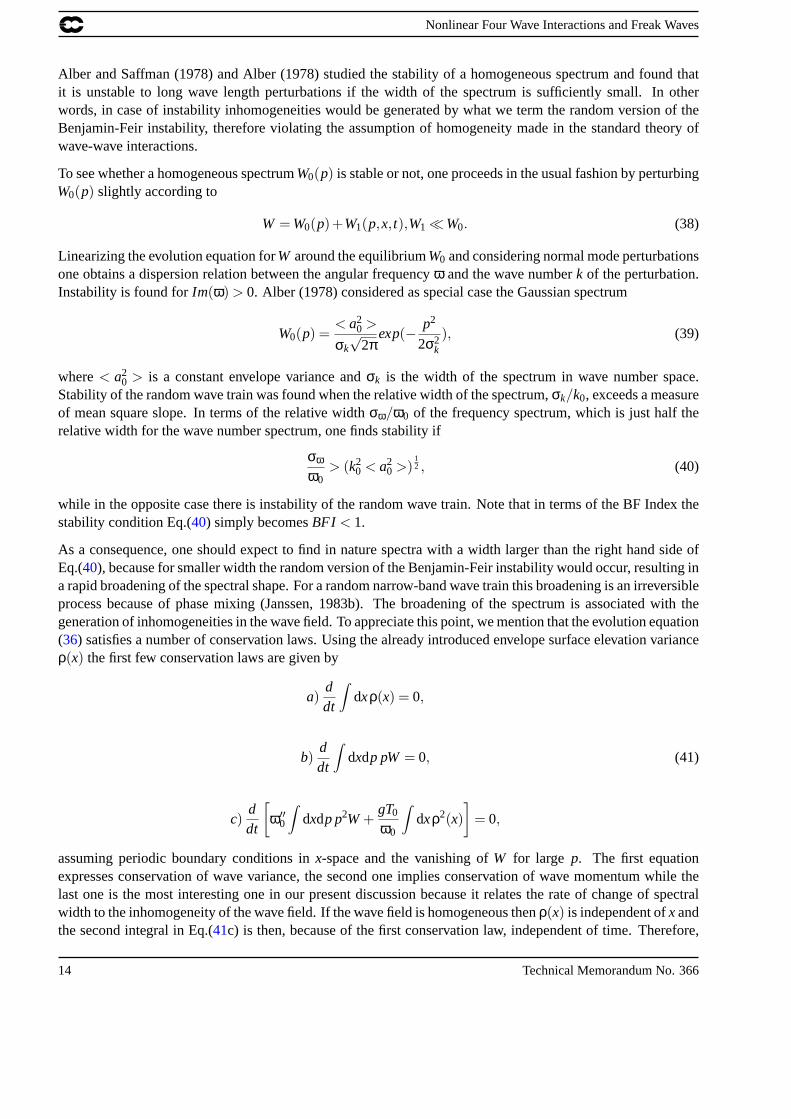
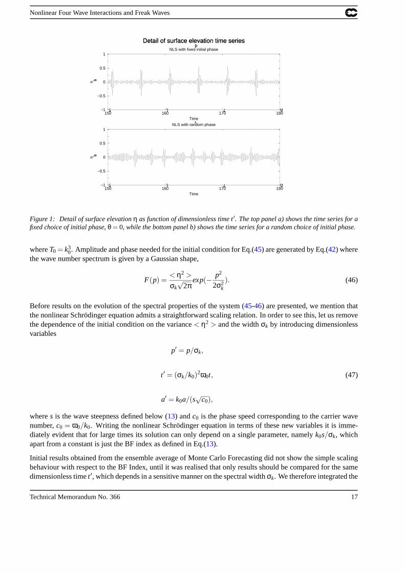
�
Figure 1: Detail of surface elevationη as function of dimensionless time t′. The top panel a) shows the time series for afixed choice of initial phase,θ = 0, while the bottom panel b) shows the time series for a random choice of initial phase.
whereT0 = k30. Amplitude and phase needed for the initial condition for Eq.(45) are generated by Eq.(42) where
the wave number spectrum is given by a Gaussian shape,
F(p) =< η2 >
σk√
2πexp(− p2
2σ2k
). (46)
Before results on the evolution of the spectral properties of the system (45-46) are presented, we mention thatthe nonlinear Schrodinger equation admits a straightforward scaling relation. In order to see this, let us removethe dependence of the initial condition on the variance< η2 > and the widthσk by introducing dimensionlessvariables
p′ = p/σk,
t ′ = (σk/k0)2ω0t, (47)
a′ = k0a/(s√
c0),
wheres is the wave steepness defined below (13) andc0 is the phase speed corresponding to the carrier wavenumber,c0 = ω0/k0. Writing the nonlinear Schrodinger equation in terms of these new variables it is imme-diately evident that for large times its solution can only depend on a single parameter, namelyk0s/σk, whichapart from a constant is just the BF index as defined in Eq.(13).
Initial results obtained from the ensemble average of Monte Carlo Forecasting did not show the simple scalingbehaviour with respect to the BF Index, until it was realised that only results should be compared for the samedimensionless timet ′, which depends in a sensitive manner on the spectral widthσk. We therefore integrated the
Technical Memorandum No. 366 17

Nonlinear Four Wave Interactions and Freak Waves
−5.0 −3.0 −1.0 1.0 3.0 5.0x/sqrt(m_0)
0.0
0.2
0.4
0.6
0.8
1.0
PD
F
PDF of surface elevationNLS
GaussianPhase=0Random Phase
Figure 2: The surface elevation probability distribution as function of normalized height,η/√
m0 (with m0 the variance),corresponding to the cases of Fig. 1. For reference the Gaussian distribution is shown as well.
system of equations (45) until a fixed dimensionless timet ′ = 15. A spectral widthσk = 0.2k0 was chosen andwithout loss of generality the carrier wave numberk0 = 1 was taken. The integration interval then correspondsto about 60 wave peak periods. Furthermore, the resolution in wave number space was taken as∆k = σk/3while the total number of wave components was 41, therefore covering a wide range in wave number space. Asalready noted this choice gave for linear waves a reasonable simulation of the pdf of the surface elevation.
We remark that the specification of a random initial phase has important consequences for the evolution of anarrow-band wave train. This is immediately evident when we compare in Fig. 1 time series for the surfaceelevation from a run with a fixed initial phaseθ(k) = 0 with results from a run with a random choice of theinitial phase. While with a deterministic choice of initial phase the nonlinear Schrodinger equation generatesin an almost periodic fashion extreme events (Fig. 1a), satisfying the criteria for freak waves, with a randomchoice of initial phase (Fig. 1b) this is much less evident. Comparing the timeseries from the two cases indetail it is clear that for fixed phase small waves and large waves occurr more frequently than in the randomphase case. This impression is confirmed by the pdf of the surface elevation shown in Fig. 2. For referencewe have also shown the Gaussian probability distribution. In both cases there are considerable deviations fromNormality, but in particular for deterministic phase the deviations are large. Similar deviations from the Normaldistribution were found by Janssen and Komen (1982). Their approach was entirely analytical and they startedfrom the assumption that for large time the solution of the nonlinear Schrodinger equation would evolve towardsa series of envelope solitons, described by an elliptic function. Although they only considered the pdf of theenvelope (which under normal conditions is given by the Rayleigh Distribution), one may obtain the pdf ofthe surface elevation as well. The resulting analytical pdf has similar characteristics as the pdf for the case ofdeterministic phase.
The Monte Carlo approach was adopted because it is not evident that for the system under discussion the ergodichypothesis applies. This hypothesis implies replacement of the ensemble average by a time average. However,if one happens to choose initial phases in a way that is favourable for the generation of envelope solitons, thenthere is a high probability that the solution stays close to the envelope soliton branch and will hardly ever visitother parts of phase space. In order to guarantee a representative picture we therefore decided to performNens
runs where for each run amplitude and phase are drawn in an independent manner. In the remainder, onlyensemble averaged results will be discussed.
18 Technical Memorandum No. 366
Nonlinear Four Wave Interactions and Freak Waves
0.0 5.0 10.0 15.0 20.0Time
0.20
0.30
0.40
Spe
ctra
l Wid
th
Time evolution of Spectral WidthNLS; n_modes = 41 (focussing)
BFI=0.4BFI=1.0BFI=1.4BFI=2.0Theory
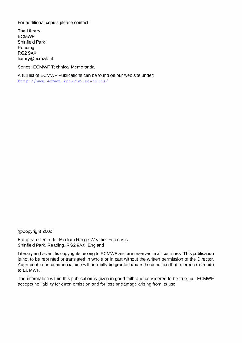
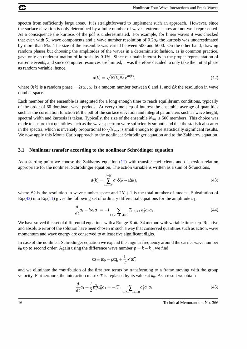
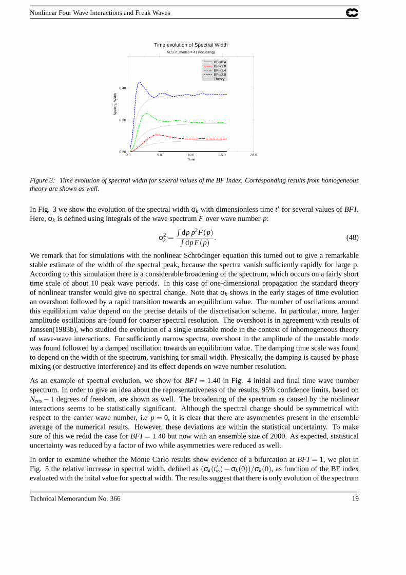
Figure 3: Time evolution of spectral width for several values of the BF Index. Corresponding results from homogeneoustheory are shown as well.
In Fig. 3 we show the evolution of the spectral widthσk with dimensionless timet ′ for several values ofBFI.Here,σk is defined using integrals of the wave spectrumF over wave numberp:
σ2k =
∫dp p2F(p)∫dp F(p)
. (48)
We remark that for simulations with the nonlinear Schrodinger equation this turned out to give a remarkablestable estimate of the width of the spectral peak, because the spectra vanish sufficiently rapidly for large p.According to this simulation there is a considerable broadening of the spectrum, which occurs on a fairly shorttime scale of about 10 peak wave periods. In this case of one-dimensional propagation the standard theoryof nonlinear transfer would give no spectral change. Note thatσk shows in the early stages of time evolutionan overshoot followed by a rapid transition towards an equilibrium value. The number of oscilations aroundthis equilibrium value depend on the precise details of the discretisation scheme. In particular, more, largeramplitude oscillations are found for coarser spectral resolution. The overshoot is in agreement with results ofJanssen(1983b), who studied the evolution of a single unstable mode in the context of inhomogeneous theoryof wave-wave interactions. For sufficiently narrow spectra, overshoot in the amplitude of the unstable modewas found followed by a damped oscillation towards an equilibrium value. The damping time scale was foundto depend on the width of the spectrum, vanishing for small width. Physically, the damping is caused by phasemixing (or destructive interference) and its effect depends on wave number resolution.
As an example of spectral evolution, we show forBFI = 1.40 in Fig. 4 initial and final time wave numberspectrum. In order to give an idea about the representativeness of the results, 95% confidence limits, based onNens−1 degrees of freedom, are shown as well. The broadening of the spectrum as caused by the nonlinearinteractions seems to be statistically significant. Although the spectral change should be symmetrical withrespect to the carrier wave number, i.ep = 0, it is clear that there are asymmetries present in the ensembleaverage of the numerical results. However, these deviations are within the statistical uncertainty. To makesure of this we redid the case forBFI = 1.40 but now with an ensemble size of 2000. As expected, statisticaluncertainty was reduced by a factor of two while asymmetries were reduced as well.
In order to examine whether the Monte Carlo results show evidence of a bifurcation atBFI = 1, we plot inFig. 5 the relative increase in spectral width, defined as(σk(t ′∞)−σk(0))/σk(0), as function of the BF indexevaluated with the inital value for spectral width. The results suggest that there is only evolution of the spectrum
Technical Memorandum No. 366 19

Nonlinear Four Wave Interactions and Freak Waves
−1.5 −0.5 0.5 1.5k
0.000
0.005
0.010
0.015
0.020
0.025
F(k
)
Wavenumber SpectrumNLS; BFI=1.4; n_modes = 41 (focussing)
Initial SpectrumFinal Spectrum(MCFW)Final Spectrum(Theory)
Figure 4: Initial and final time wave number spectrum according to the Monte Carlo Forecasting of Waves (MCFW)using the nonlinear Schrodinger Equation. Error bars give95%confidence limits. Results from theory are shown as well.
0.0 1.0 2.0 3.0 4.0BFI
0.0
0.5
1.0
1.5
2.0
∆(σ)
/σ
Relative Spectral Broadening versus BF IndexNLS; n_modes = 41
MCFW (BF)Theory (BF)MCFW (no BF)Theory (no BF)
Figure 5: Relative spectral broadening(σk(t ′∞)− σk(0))/σk(0) as function of the BF Index. Shown are results forfocussing (BF) and defocussing (no BF) from the simulations and from theory, but results from theory are identical forthese two cases.
20 Technical Memorandum No. 366
Nonlinear Four Wave Interactions and Freak Waves
0.0 1.0 2.0 3.0 4.0BFI(t=0)
0.0
0.5
1.0
1.5
2.0
BF
I(t=
15)
Final time versus Initial BF IndexNLS; n_modes = 41
MCFW (BF)Theory (BF)MCFW (no BF)Theory (no BF)
Figure 6: Final time versus initial time value of the BF Index for the same cases as displayed in Fig. 5.
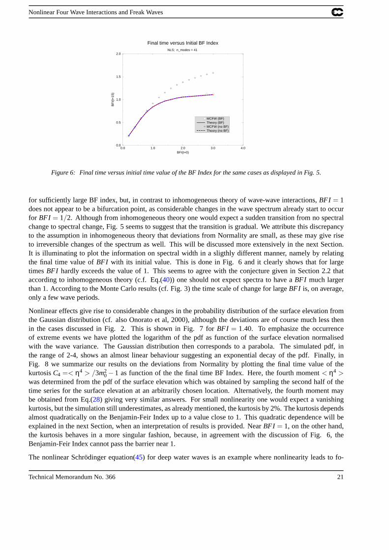
for sufficiently large BF index, but, in contrast to inhomogeneous theory of wave-wave interactions,BFI = 1does not appear to be a bifurcation point, as considerable changes in the wave spectrum already start to occurfor BFI = 1/2. Although from inhomogeneous theory one would expect a sudden transition from no spectralchange to spectral change, Fig. 5 seems to suggest that the transition is gradual. We attribute this discrepancyto the assumption in inhomogeneous theory that deviations from Normality are small, as these may give riseto irreversible changes of the spectrum as well. This will be discussed more extensively in the next Section.It is illuminating to plot the information on spectral width in a sligthly different manner, namely by relatingthe final time value ofBFI with its initial value. This is done in Fig. 6 and it clearly shows that for largetimesBFI hardly exceeds the value of 1. This seems to agree with the conjecture given in Section 2.2 thataccording to inhomogeneous theory (c.f. Eq.(40)) one should not expect spectra to have aBFI much largerthan 1. According to the Monte Carlo results (cf. Fig. 3) the time scale of change for largeBFI is, on average,only a few wave periods.
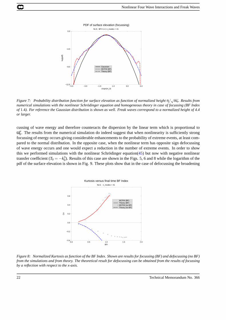
Nonlinear effects give rise to considerable changes in the probability distribution of the surface elevation fromthe Gaussian distribution (cf. also Onorato et al, 2000), although the deviations are of course much less thenin the cases discussed in Fig. 2. This is shown in Fig. 7 forBFI = 1.40. To emphasize the occurrenceof extreme events we have plotted the logarithm of the pdf as function of the surface elevation normalisedwith the wave variance. The Gaussian distribution then corresponds to a parabola. The simulated pdf, inthe range of 2-4, shows an almost linear behaviour suggesting an exponential decay of the pdf. Finally, inFig. 8 we summarize our results on the deviations from Normality by plotting the final time value of thekurtosisC4 =< η4 > /3m2
0−1 as function of the the final time BF Index. Here, the fourth moment< η4 >was determined from the pdf of the surface elevation which was obtained by sampling the second half of thetime series for the surface elevation at an arbitrarily chosen location. Alternatively, the fourth moment maybe obtained from Eq.(28) giving very similar answers. For small nonlinearity one would expect a vanishingkurtosis, but the simulation still underestimates, as already mentioned, the kurtosis by 2%. The kurtosis dependsalmost quadratically on the Benjamin-Feir Index up to a value close to 1. This quadratic dependence will beexplained in the next Section, when an interpretation of results is provided. NearBFI = 1, on the other hand,the kurtosis behaves in a more singular fashion, because, in agreement with the discussion of Fig. 6, theBenjamin-Feir Index cannot pass the barrier near 1.
The nonlinear Schrodinger equation(45) for deep water waves is an example where nonlinearity leads to fo-
Technical Memorandum No. 366 21
Nonlinear Four Wave Interactions and Freak Waves
−5.0 −3.0 −1.0 1.0 3.0 5.0x/sqrt(m_0)
−12.0
−8.0
−4.0
0.0
log(
pdf)
PDF of surface elevation (focussing)NLS; BFI=1.4; n_modes = 41
GaussianMCFW (BF)Theory (BF)
Figure 7: Probability distribution function for surface elevation as function of normalized heightη/√
m0. Results fromnumerical simulations with the nonlinear Schrodinger equation and homogeneous theory in case of focussing (BF Indexof 1.4). For reference the Gaussian distribution is shown as well. Freak waves correspond to a normalized height of 4.4or larger.
cussing of wave energy and therefore counteracts the dispersion by the linear term which is proportional toω′′0. The results from the numerical simulation do indeed suggest that when nonlinearity is sufficiently strongfocussing of energy occurs giving considerable enhancements to the probability of extreme events, at least com-pared to the normal distribution. In the opposite case, when the nonlinear term has opposite sign defocussingof wave energy occurs and one would expect a reduction in the number of extreme events. In order to showthis we performed simulations with the nonlinear Schrodinger equation(45) but now with negative nonlineartransfer coefficient (T0 =−k3
0). Results of this case are shown in the Figs. 5, 6 and 8 while the logarithm of thepdf of the surface elevation is shown in Fig. 9. These plots show that in the case of defocussing the broadening
0.0 0.5 1.0 1.5 2.0BFI
−0.4
−0.2
0.0
0.2
0.4
0.6
C4
Kurtosis versus final time BF IndexNLS; n_modes = 41
MCFW (BF)Theory (BF)MCFW (no BF)Theory (no BF)
Figure 8: Normalized Kurtosis as function of the BF Index. Shown are results for focussing (BF) and defocussing (no BF)from the simulations and from theory. The theoretical result for defocussing can be obtained from the results of focussingby a reflection with respect to the x-axis.
22 Technical Memorandum No. 366

Nonlinear Four Wave Interactions and Freak Waves
−5.0 −3.0 −1.0 1.0 3.0 5.0x/sqrt(m_0)
−12.0
−8.0
−4.0
0.0
log(
pdf)
PDF of surface elevation (defocussing)NLS; BFI=1.4; n_modes = 41
GaussianMCFW (no BF)Theory (no BF)
Figure 9: Probability distribution function for surface elevation as function of normalized heightη/√
m0. Results fromnumerical simulations with the nonlinear Schrodinger equation and homogeneous theory in case of defocussing (BF Indexof 1.4). For reference the Gaussian distribution is shown as well.
of the spectrum is less dramatic. Furthermore, the final time Benjamin-Feir Index does not have a limitingvalue of about 1. On the other hand, the kurtosis for this case is negative, resulting, as can be seen from Fig.9, in a large reduction of the probability of extreme events. The dependence of the kurtosis onBFI is differentfrom the case of focussing, because there are clear signs of saturation beyondBFI = 1, while only in the rangeBFI < 0.5 there is a quadratic dependence of kurtosisC4 onBFI.
3.2 Nonlinear transfer according to the Zakharov Equation
The nonlinear Schrodinger equation gives the lowest order effects of finite bandwidth on the evolution of aweakly nonlinear wave train. Dysthe (1979) investigated the consequences of next order in bandwidth and hefound a surprisingly large impact on the results for the growth rates of the modulational instability. Similarly,Crawford et al (1981) studied the stability of a uniform wave train using the complete Zakharov equation whichretains all the high-order dispersion effects. In general, growth rates are reduced compared to results fromthe nonlinear Schrodinger equation, therefore according to the Zakharov and the Dysthe equation a uniformwave train is less unstable. In fact, growth rates and thresholds for instability were in better agreement withexperimental results of Benjamin & Feir (1967) and Lake et al (1977) (cf. also Janssen, 1983a). The Zakharovand the Dysthe equation have, in addition, the interesting property that the nonlinear transfer coefficient and theangular frequencies are not symmetrical with respect to the carrier wave number. It will be seen that this hasimportant consequences for the spectral shape.
The Dysthe equation follows from the Zakharov equation by expanding angular frequency to third order in themodulation wave numberp while the interaction matrixT is expanded up to first order inp. For narrow-bandwave trains it gives an accurate description of the sea state. However, wave spectra may become so broad thatthe narrow-band approximation becomes invalid, and therefore we have chosen to study numerical results fromthe Zakharov equation.
The Zakharov equation we solved was given by Eq.(44), where the nonlinear transfer coefficient was fromKrasitskii (1990), while the exact dispersion relation for deep water gravity waves was taken. The initial con-dition was provided by Eq.(46). The discretisation details were identical to those of the numerical simulations
Technical Memorandum No. 366 23
Nonlinear Four Wave Interactions and Freak Waves
0.0 1.0 2.0 3.0k
0.000
0.005
0.010
0.015
0.020
F(k
)
Wavenumber SpectrumZakharov Eq.; BFI=1.4; n_modes = 41
Initial SpectrumFinal Spectrum(MCFW) Final Spectrum(Theory)
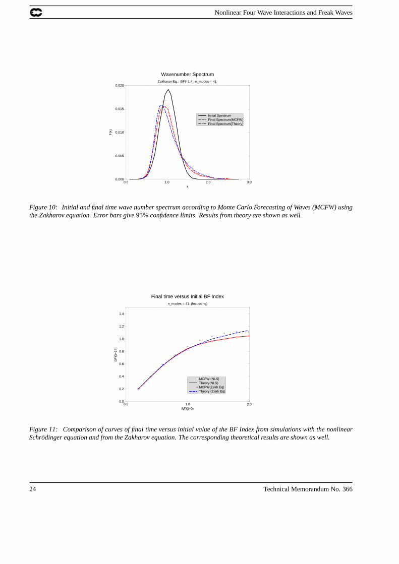
Figure 10: Initial and final time wave number spectrum according to Monte Carlo Forecasting of Waves (MCFW) usingthe Zakharov equation. Error bars give95%confidence limits. Results from theory are shown as well.
0.0 1.0 2.0BFI(t=0)
0.0
0.2
0.4
0.6
0.8
1.0
1.2
1.4
BF
I(t=
15)
Final time versus Initial BF Indexn_modes = 41 (focussing)
MCFW (NLS)Theory(NLS)MCFW(Zakh Eq)Theory (Zakh Eq)
Figure 11: Comparison of curves of final time versus initial value of the BF Index from simulations with the nonlinearSchrodinger equation and from the Zakharov equation. The corresponding theoretical results are shown as well.
24 Technical Memorandum No. 366
Nonlinear Four Wave Interactions and Freak Waves
with the nonlinear Schrodinger equation. Because the Zakharov equation contains all higher-order terms in themodulation wave number p it is not possible to prove that the large time solution of the initial value problemis determined completely by the BF Index, but in good approximation the BF Index can still be used for thispurpose as long as the spectra are narrow-banded.
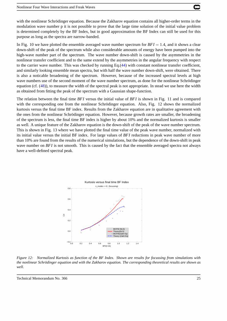
In Fig. 10 we have plotted the ensemble averaged wave number spectrum forBFI = 1.4, and it shows a cleardown-shift of the peak of the spectrum while also considerable amounts of energy have been pumped into thehigh-wave number part of the spectrum. The wave number down-shift is caused by the asymmetries in thenonlinear transfer coefficient and to the same extend by the asymmetries in the angular frequency with respectto the carrier wave number. This was checked by running Eq.(44) with constant nonlinear transfer coefficient,and similarly looking ensemble mean spectra, but with half the wave number down-shift, were obtained. Thereis also a noticable broadening of the spectrum. However, because of the increased spectral levels at highwave numbers use of the second moment of the wave number spectrum, as done for the nonlinear Schrodingerequation (cf. (48)), to measure the width of the spectral peak is not appropriate. In stead we use here the widthas obtained from fitting the peak of the spectrum with a Gaussian shape-function.
The relation between the final timeBFI versus the initial value ofBFI is shown in Fig. 11 and is comparedwith the corresponding one from the nonlinear Schrodinger equation. Also, Fig. 12 shows the normalizedkurtosis versus the final time BF index. Results from the Zakharov equation are in qualitative agreement withthe ones from the nonlinear Schrodinger equation. However, because growth rates are smaller, the broadeningof the spectrum is less, the final time BF index is higher by about 10% and the normalized kurtosis is smalleras well. A unique feature of the Zakharov equation is the down-shift of the peak of the wave number spectrum.This is shown in Fig. 13 where we have plotted the final time value of the peak wave number, normalized withits initial value versus the initial BF index. For large values ofBFI reductions in peak wave number of morethan 10% are found from the results of the numerical simulations, but the dependence of the down-shift in peakwave number onBFI is not smooth. This is caused by the fact that the ensemble averaged spectra not alwayshave a well-defined spectral peak.
0.0 0.2 0.4 0.6 0.8 1.0 1.2 1.4BFI(t=15)
−0.2
0.0
0.2
0.4
0.6
0.8
C4
Kurtosis versus final time BF Indexn_modes = 41 (focussing)
MCFW (NLS)Theory(NLS)MCFW(Zakh Eq)Theory (Zakh Eq)
Figure 12: Normalized Kurtosis as function of the BF Index. Shown are results for focussing from simulations withthe nonlinear Schrodinger equation and with the Zakharov equation. The corresponding theoretical results are shown aswell.
Technical Memorandum No. 366 25
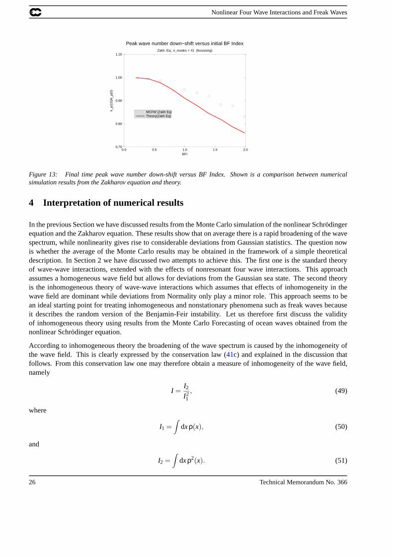
Nonlinear Four Wave Interactions and Freak Waves
0.0 0.5 1.0 1.5 2.0BFI
0.70
0.80
0.90
1.00
1.10
k_p(
15)/
k_p(
0)
Peak wave number down−shift versus initial BF IndexZakh. Eq.; n_modes = 41 (focussing)
MCFW (Zakh Eq)Theory(Zakh Eq)
Figure 13: Final time peak wave number down-shift versus BF Index. Shown is a comparison between numericalsimulation results from the Zakharov equation and theory.
4 Interpretation of numerical results
In the previous Section we have discussed results from the Monte Carlo simulation of the nonlinear Schrodingerequation and the Zakharov equation. These results show that on average there is a rapid broadening of the wavespectrum, while nonlinearity gives rise to considerable deviations from Gaussian statistics. The question nowis whether the average of the Monte Carlo results may be obtained in the framework of a simple theoreticaldescription. In Section 2 we have discussed two attempts to achieve this. The first one is the standard theoryof wave-wave interactions, extended with the effects of nonresonant four wave interactions. This approachassumes a homogeneous wave field but allows for deviations from the Gaussian sea state. The second theoryis the inhomogeneous theory of wave-wave interactions which assumes that effects of inhomogeneity in thewave field are dominant while deviations from Normality only play a minor role. This approach seems to bean ideal starting point for treating inhomogeneous and nonstationary phenomena such as freak waves becauseit describes the random version of the Benjamin-Feir instability. Let us therefore first discuss the validityof inhomogeneous theory using results from the Monte Carlo Forecasting of ocean waves obtained from thenonlinear Schrodinger equation.
According to inhomogeneous theory the broadening of the wave spectrum is caused by the inhomogeneity ofthe wave field. This is clearly expressed by the conservation law (41c) and explained in the discussion thatfollows. From this conservation law one may therefore obtain a measure of inhomogeneity of the wave field,namely
I =I2I21
, (49)
where
I1 =∫
dxρ(x), (50)
and
I2 =∫
dxρ2(x). (51)
26 Technical Memorandum No. 366
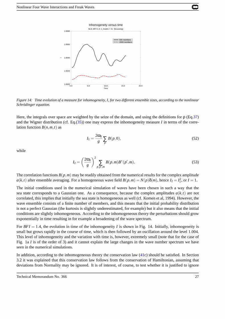
Nonlinear Four Wave Interactions and Freak Waves
0.0 5.0 10.0 15.0 20.0Time
1.0000
1.0020
1.0040
1.0060
1.0080
I
Inhomogeneity versus timeNLS; BFI=1.4; n_modes = 41 (focussing)
500 members2000 members
Figure 14: Time evolution of a measure for inhomogeneity, I, for two different ensemble sizes, according to the nonlinearSchrodinger equation.
Here, the integrals over space are weighted by the seize of the domain, and using the definitions forρ (Eq.37)and the Wigner distribution (cf. Eq.(35)) one may express the inhomogeneity measureI in terms of the corre-lation functionB(n,m, t) as
I1 =2ω0
g ∑p
B(p,0), (52)
while
I2 =(
2ω0
g
)2
∑p,p′,m
B(p,m)B∗(p′,m), (53)
The correlation functionsB(p,m) may be readily obtained from the numerical results for the complex amplitudea(k, t) after ensemble averaging. For a homogeneous wave fieldB(p,m) = N(p)δ(m), henceI2 = I2
1, or I = 1.
The initial conditions used in the numerical simulation of waves have been chosen in such a way that thesea state corresponds to a Gaussian one. As a consequence, because the complex amplitudesa(k, t) are notcorrelated, this implies that initially the sea state is homogeneous as well (cf. Komen et al, 1994). However, thewave ensemble consists of a finite number of members, and this means that the initial probability distributionis not a perfect Gaussian (the kurtosis is slightly underestimated, for example) but it also means that the initialconditions are slightly inhomogeneous. According to the inhomogeneous theory the perturbations should growexponentially in time resulting in for example a broadening of the wave spectrum.
For BFI = 1.4, the evolution in time of the inhomogeneityI is shown in Fig. 14. Initially, inhomogeneity issmall but grows rapidly in the course of time, which is then followed by an oscillation around the level 1.004.This level of inhomogeneity and the variation with time is, however, extremely small (note that for the case ofFig. 1aI is of the order of 3) and it cannot explain the large changes in the wave number spectrum we haveseen in the numerical simulations.
In addition, according to the inhomogeneous theory the conservation law (41c) should be satisfied. In Section3.2 it was explained that this conservation law follows from the conservation of Hamiltonian, assuming thatdeviations from Normality may be ignored. It is of interest, of course, to test whether it is justified to ignore
Technical Memorandum No. 366 27
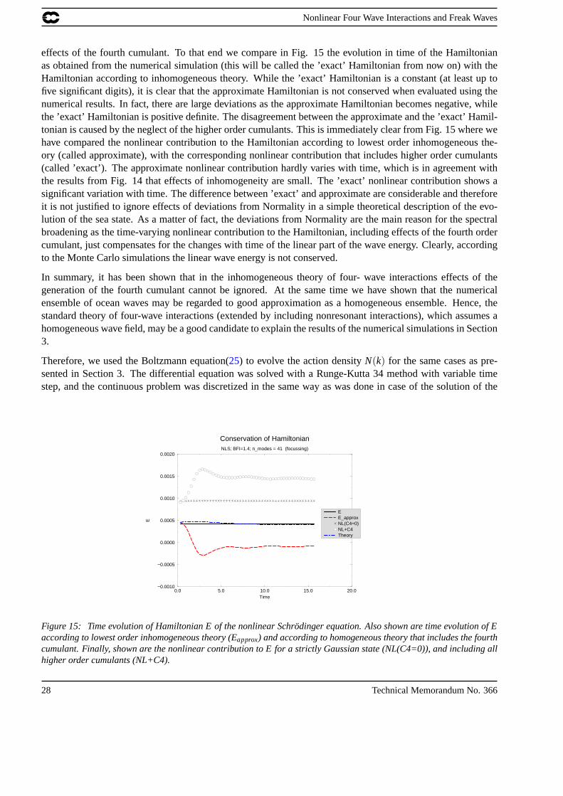
Nonlinear Four Wave Interactions and Freak Waves
effects of the fourth cumulant. To that end we compare in Fig. 15 the evolution in time of the Hamiltonianas obtained from the numerical simulation (this will be called the ’exact’ Hamiltonian from now on) with theHamiltonian according to inhomogeneous theory. While the ’exact’ Hamiltonian is a constant (at least up tofive significant digits), it is clear that the approximate Hamiltonian is not conserved when evaluated using thenumerical results. In fact, there are large deviations as the approximate Hamiltonian becomes negative, whilethe ’exact’ Hamiltonian is positive definite. The disagreement between the approximate and the ’exact’ Hamil-tonian is caused by the neglect of the higher order cumulants. This is immediately clear from Fig. 15 where wehave compared the nonlinear contribution to the Hamiltonian according to lowest order inhomogeneous the-ory (called approximate), with the corresponding nonlinear contribution that includes higher order cumulants(called ’exact’). The approximate nonlinear contribution hardly varies with time, which is in agreement withthe results from Fig. 14 that effects of inhomogeneity are small. The ’exact’ nonlinear contribution shows asignificant variation with time. The difference between ’exact’ and approximate are considerable and thereforeit is not justified to ignore effects of deviations from Normality in a simple theoretical description of the evo-lution of the sea state. As a matter of fact, the deviations from Normality are the main reason for the spectralbroadening as the time-varying nonlinear contribution to the Hamiltonian, including effects of the fourth ordercumulant, just compensates for the changes with time of the linear part of the wave energy. Clearly, accordingto the Monte Carlo simulations the linear wave energy is not conserved.
In summary, it has been shown that in the inhomogeneous theory of four- wave interactions effects of thegeneration of the fourth cumulant cannot be ignored. At the same time we have shown that the numericalensemble of ocean waves may be regarded to good approximation as a homogeneous ensemble. Hence, thestandard theory of four-wave interactions (extended by including nonresonant interactions), which assumes ahomogeneous wave field, may be a good candidate to explain the results of the numerical simulations in Section3.
Therefore, we used the Boltzmann equation(25) to evolve the action densityN(k) for the same cases as pre-sented in Section 3. The differential equation was solved with a Runge-Kutta 34 method with variable timestep, and the continuous problem was discretized in the same way as was done in case of the solution of the
0.0 5.0 10.0 15.0 20.0Time
−0.0010
−0.0005
0.0000
0.0005
0.0010
0.0015
0.0020
E
Conservation of HamiltonianNLS; BFI=1.4; n_modes = 41 (focussing)
EE_approxNL(C4=0)NL+C4Theory
Figure 15: Time evolution of Hamiltonian E of the nonlinear Schrodinger equation. Also shown are time evolution of Eaccording to lowest order inhomogeneous theory (Eapprox) and according to homogeneous theory that includes the fourthcumulant. Finally, shown are the nonlinear contribution to E for a strictly Gaussian state (NL(C4=0)), and including allhigher order cumulants (NL+C4).
28 Technical Memorandum No. 366
Nonlinear Four Wave Interactions and Freak Waves
Zakharov equation. Run times using the homogeneous theory are typically two orders of magnitudes fasterthan when following the ensemble approach.
In contrast to inhomogeneous theory, the standard theory gives a much better approximation to the ’exact’Hamiltonian as shown in Fig. 15. There are, as should be, small differences because the standard theory isan approximation as well, since both effects of inhomogeneity and the sixth cumulant have been neglected.Further results from the discretized version of the homogeneous theory are compared with the ones from thesimulations with the nonlinear Schrodinger equation in the Figs. 3-8.
From Fig. 3 which shows the evolution in time of the spectral width for several values of the Benjamin-FeirIndex it is seen that for large times there is good agreement between homogeneous theory and the ensembleaveraged results from the Monte Carlo simulations. For short times it is however evident that Eq.(25) doesnot show the overshoot found in the numerical simulations. A likely reason for the absence of overshoot inthe theoretical calculations is the assumption that the action density varies slowly compared to the time scaleimplied by the resonance functionRi(∆ω, t). Both the numerical simulations and homogeneous theory showon the one hand for short times a rapid broadening of the wave spectrum which for large times is followedby a transition towards a steady state. The evolution towards a steady state can be understood as follows:First, it should be noted that, according to Section 2.3, for one-dimensional propagation there is no nonlineartransfer due to resonant nonlinear interactions. Now, initially the resonance functionRi(∆ω, t) will be wide sothat nonresonant wave-wave interactions are allowed to modify the action density spectrum. But after about5-10 wave periods the resonance function becomes progressively narrower until it becomes approximately aδ-function, hence only resonant waves are selected. In that event there is no change of the action density spectrumpossible anymore so that for large times a steady state is achieved.
A example of the comparison between theoretical and simulated spectrum is given in Fig. 4. There is a fairagreement between the two. However, it should be mentioned that typically the simulated spectrum is slightlymore peaked than the theoretical one despite the fact that there is a close agreement in spectral width. Thisagreement in spectral width between theory and simulation is also very much evident in the Figs. 5 and 6 overthe full range of the initial value ofBFI. In particular note that there is close agreement between the upper limitof the final timeBFI from theory and the simulation. Hence, homogeneous theory also provides an explanationof why there is a lower bound to spectral width.
We therefore have the curious situation that both homogeneous and inhomogeneous theory explain why thereis a lower bound to spectral width as found in the numerical simulations. However, since it has been shown thatinhomogeneities only play a minor role in the numerical simulations it follows that only homogeneous theoryprovides a proper explanation. In-situ observations from the North Sea seem to indicate the presence of a lowerbound to spectral width as well (see for example Janssen, 1991). Although it is impossible to prove at presentthat at sea inhomogeneities do not play a role, homogeneous theory even seems to give a plausible explanationof the lower bound found at sea.
As discussed in Section 2.3 nonlinearity gives rise to deviations from the normal distribution. We determinedthe normalised kurtosis using Eq.(29), which is obtained from the fourth cumulantD. Introducing the normal-ized heightx = η/
√m0, the pdf of the normalized surface elevationx is then given by
p(x) =(
1+18
C4d4
dx4
)f0, (54)
where f0 is given by the normal distribution
f0(x) =1√2π
exp(−x2
2). (55)
Technical Memorandum No. 366 29
Nonlinear Four Wave Interactions and Freak Waves
Eq.(54) follows from an expansion of the pdfp in terms of orthogonal functions(d/dx)n f0. Here, n is evenbecause of the symmetry of the Zakharov equation. The expansion coefficients are then obtained by determiningthe first, second and fourth moment. For the range ofBFI studied in this paper it was verified that highermoments only gave a small contribution to the shape of the pdfp(x). The pdf according to theory is compared inFig. 7 with the simulated one, and a good agreement is obtained, even for extreme sea state conditions. Clearlyin the case of nonlinear focussing, the probability of extreme states is, as expected, larger when compared tothe normal distribution. Finally, in Fig. 8 theoretical and simulated final time kurtosis is plotted as function ofthe final timeBFI. A good agreement between the two results is obtained even close to the limiting value ofthe final timeBFI. ForBFI < 1 both simulated and theoretical kurtosis depend in an almost quadratic fashiononBFI, in agreement with the simple estimates ofC4 given in Section 2.3 (cf Eq.(31)).
In the case of nonlinear focussing a good agreement between the numerical simulations and the homogeneoustheory has been obtained, even for extreme values of the Benjamin-Feir Index. Here, it should be emphasizedthat at seaBFI has typical values of 0.5 or less and only occasionaly values of the order 1 are reached. We haveperformed simulations to values ofBFI of up to 3 and even for these extreme conditions, having large values ofkurtosis for example, a reasonable agreement is obtained. This is surprising because the homogeneous theorywas derived under the assumption of small deviations from Normality.
In the case of nonlinear defocussing the range of validity of homogeneous theory is much more restricted.This is made plainly clear in the Figs. 5, 6, 8 and 9, where results from the simulations and homogeneoustheory are compared for the case of nonlinear defocussing. In order to be able to interpret this comparison wenote that homogeneous theory does not distinguish between focussing and defocusing because the nonlineartransfer is independent of the sign of the interaction matrixT. Only the kurtosis depends on the sign ofT.Judging from the Figs. 5, 6 and 8 the range of validity of homogeneous theory is restricted toBFI < 0.6.In particularly, for largeBFI there are large qualitative deviations in the kurtosis of the pdf: while from thenumerical simulations there are clear signs of saturation in kurtosis, there is no indication of saturation in theresults from homogeneous theory. In addition, in case of nonlinear defocussing the kurtosis is negative sothat for large normalized elevationx the pdf given in Eq.(54) may become negative. This is clearly unrealisticand in order to correct this undesirable property of homogeneous theory one needs, for largeBFI, to take intoaccount the effects of higher then fourth order cumulants as well. It is believed this is the main reason whyhomogeneous theory has such a restricted validity in this case. In the opposite case of nonlinear focussingthe kurtosis is positive, giving for largex a positive correction to the normal distribution. The pdf of thesurface elevation is therefore positive, at least for the cases that have been studied here, and as a consequencehomogeneous theory has a much larger range of validity.
Finally, we applied homogeneous theory to the Zakharov equation. Results are compared with the numericalsimulations in the Figs. 10, 11, 12 and 13. There is a fair agreement between simulated and theoretical spectrum(cf. Fig. 10), between simulated and theoretical final timeBFI index (cf. Fig. 11) and normalized kurtosis(cf. Fig. 12). Less favourable is the agreement between simulated and theoretical peak wave number, as showin Fig. 13. The theoretical results show a smooth dependence of wave-number down-shift onBFI, givingshifts of 20% or more for large values ofBFI. However, the simulation shows more scatter while the down-shift is at most 15%. The reason for the scatter in the simulated results is probably that the peak of the wavenumber spectrum is not always well-defined. In contrast, homogeneous theory gives a smoother spectrum anda well-defined peak of the spectrum.
30 Technical Memorandum No. 366

Nonlinear Four Wave Interactions and Freak Waves
5 Conclusions
Present day wave forecasting systems are based on a description of the ensemble averaged sea state. In thisapproach the wave number spectrum plays a central role and its evolution follows from the energy balanceequation. The question discussed here is whether it is possible to make statements, necessarily of a statisticalnature, on the occurence of extreme events such as freak waves.
In order to show that this is possible the following approach has been adopted. The starting point is a deter-ministic set of equations, namely the Zakharov equation or its narrow-band limit the nonlinear Schrodingerequation. There is ample evidence that these equations admit freak wave type solutions. These freak waves oc-cur when the waves are sufficiently steep as nonlinear focussing may then overcome the spreading of energy bylinear dispersion. For the same reason the Benjamin-Feir instability occurs. As shown in Fig. 1 the occurrenceof freak waves depends in a sensitive manner on the choice of the initial phase of the waves. In addition, onthe open ocean waves propagate from different locations towards a certain point of interest, and may thereforebe regarded as independent. Hence, for open ocean applications the random phase approximation seems to beappropriate. We therefore simulated the evolution of an ensemble of ocean waves by running a determinis-tic model with random initial phase. These Monte Carlo simulations are expensive (typically, the size of theensemble is 500) so that we restrict ourselves to the case of one-dimensional propagation only.
The ensemble average of the results from the Monte Carlo simulations shows that when the Benjamin-FeirIndex is sufficiently large (as occurs for the combination of narrow spectra and steep waves) the wave spectrumbroadens while at the same time considerable deviations from the Gaussian pdf are found. In case of theZakharov equation the spectral change is even asymetrical with respect to the peak of a symmetrical spectrumgiving a down-shift of the peak wave number while as a consequence of the conservation of wave action andwave energy considerable amounts of energy are being pumped into the high-wave number part of the spectrum.These spectral changes occur on a short time scale, typically of the order of ten wave periods. This time scaleis comparable with the Benjamin-Feir time scale.
The standard homogeneous theory of resonant nonlinear transfer does not give spectral change in the case ofone-dimensional propagation. This theory was therefore extended to allow for nonresonant interactions as well,because the nonlinear focussing related with the Benjamin-Feir Instability is an example of a nonresonant four-wave interaction. This nonlinear four-wave transfer is associated with the generation of higher order cumulantssuch as the kurtosis. Deviations of the surface elevation pdf from the normal distribution can therefore beexpressed in terms of a six-dimensional integral involving the cube of the action spectrum (cf. Eq.(29)). In caseof nonlinear focussing there is, for a large range of values of theBFI, a good agreement between the ensembleaveraged results from the numerical simulations and homogeneous theory. This is in particular true for thebroadening of the spectrum, the spectral shape and the estimation of the kurtosis. Compared to the simulations,theory overestimates, however, the peak wave number down-shift.
Homogeneous theory also explains why for one-dimensional propagation the wave spectrum evolves towards asteady state. The resonance function evolves rapidly towards aδ-function, hence for large times only resonantwave-wave interactions are selected which in one dimension do not give rise to spectral change. This is in sharpcontrast with the case of two-dimensional propagation. No trend towards a steady state is expected in that casebecause resonant four-wave interactions do contribute to a change in the spectrum.
The extended version of the homogeneous four-wave theory has two time scales, a fast one on which the nonres-onant interactions take place and a long time scale on which the resonant interactions occur. The nonresonantinteractions play a similar role as transients in the solution of an initial value problem. They are simply gen-erated because initially there is a mismatch between the choice of the probability distribution of the waves, aGaussian, and between the initial choice of the wave spectrum, representing a sea state with narrow-band, steep
Technical Memorandum No. 366 31
Nonlinear Four Wave Interactions and Freak Waves
nonlinear waves. For example, if one could choose a probability distribution function which is in equilibriumwith the nonlinear sea state (theoretically one can, by the way), then nonresonant interactions would not con-tribute. Only resonant wave-wave interactions will then give rise to nonlinear transfer. In the general case forwhich there is a finite mismatch between pdf and wave spectrum, the nonresonant contribution will die out veryquickly owing to phase mixing, but will, nevertheless, as we have seen, result in considerable changes in thewave spectrum. The question therefore is whether there is a need to include effects of nonresonant interactions.This depends on the application. In wave tank experiments, where one can program a wave maker to producethe initial conditions used in this paper, it seems that effects of nonresonant transfer need to be taken accountfor. For the open ocean case this is not clear. The point is that in nature the combination of steep waves and astrictly Gaussian distribution most likely does not occur. Changes in nature are expected to be more gradual sothat the mismatch between pdf and wave spectrum is small. Only when a wind starts blowing suddenly, hencefor short fetches and duration, effects of nonresonant interactions are expected to be relevant. More research inthis direction is, however, required.
The results from Monte Carlo Simulations do not provide evidence that there are significant deviations fromhomogeneity of the ensemble of waves. Deviations from Normality are found to be much more important.Nevertheless, it cannot be concluded from the present study that the inhomogeneous approach of Alber andSaffman (1978) is not relevant for real ocean waves. For example, effects of inhomogeneity might be relevantin fetch-limited, rapidly varying circumstances. However, its effects are expected to be small and therefore onlythe lowest order approximation, as given explicitely in Eq.(36), needs to be retained.
Finally, for real ocean waves not only four-wave interactions determine the evolution of the wave spectrum.Wind input and dissipation due to white-capping are relevant, and these processes may effect the kurtosis ofthe sea surface as well. However, it has been shown in this paper that in particular the nonresonant nonlineartransfer acts on a short time scale which is much shorter then the time scales associated with wind input anddissipation source functions used in wave forecasting (Komen et al, 1994). Hence, one would expect that theexpression for kurtosis found in this paper (cf Eq.(29)) should be relevant in nature. Nevertheless, nonlinearfocussing may result in steep waves. If their steepness exceeds a certain threshold one would expect a significantamount of wave breaking, thus limiting the height of these waves, and effecting the extreme statistics. Arealistic, deterministic model of wave breaking is needed to assess the importance of wave breaking in thesecircumstances. It may be more effective, however, to try to compare results from the present approach directlywith observations of extremes collected over a long period.
AcknowledgementThe author acknowledges useful and stimulating discussions with Miguel Onorato. Hispresentation during the 2001 Wise meeting in Canada gave stimulus to have a fresh look at wave-wave in-teractions and freak waves. Furthermore, the author thanks Theo van Steyn for providing the Runge-Kuttasoftware for accurate integration of a set of ordinary differential equations. Finally, the author thanks AnthonyHollingsworth and Martin Miller for critically reading the manuscript.
6 References
Alber, I.E., 1978: The effects of Randomness on the Stability of Two-dimensional Surface Wave Trains.Proc.Roy. Soc. LondonA363, 525-546.
Alber, I.E., and P.G. Saffman, 1978: Stability of Random Nonlinear Deepwater Waves with Finite BandwidthSpectra. 31326-6035-RU-)), TRW Defense and Space System Group.
32 Technical Memorandum No. 366

Nonlinear Four Wave Interactions and Freak Waves
Benjamin, T.B., and J.E. Feir, 1967: The desintegration of wavetrains on deep water. Part 1. Theory.J. FluidMech.27, 417-430.
Benney, D., and A.C. Newell, 1967: The propagation of nonlinear wave envelopes.J. Math. Phys.46, 133-139.
Caponi, E.A., P.G. Saffman, and H.C. Yuen, 1982: Instability and confined chaos in a nonlinear dispersivewave system.Phys. Fluids25, 2159-2166.
Cohen, B.I., K.M. Watson, and B.J. West, 1976: Some properties of deep water solitons.Phys. Fluids19,345-350.
Crawford, D.R., P.G. Saffman, and H.C. Yuen, 1980: Evolution of a Random Inhomogeneous Field of Nonlinear-Deep-Water Gravity Waves.Wave Motion2, 1-16.
Crawford, D.R., B.M. Lake, P.G. Saffman, and H.C. Yuen, 1981: Stability of weakly nonlinear deep-waterwaves in two and three dimensions.J. Fluid Mech.105, 177-191.
Davidson, R.C., 1972:Methods in nonlinear plasma theory. Academic Press, New York and London, 356p.
Davey, A., 1972: The propagation of a weak nonlinear wave.J. Fluid Mech., 53, 769-781.
Dean, R.G., 1990: Freak waves: A possible explanation. In A. Torum & O.T. Gudmestad (Eds.),Water WaveKinematics (pp. 609-612), Kluwer.
Draper, L., 1965: ’Freak’ ocean waves.Marine Observer35, 193-195.
Dysthe, K.B., 1979: Note on a modification to the nonlinear Schrodinger equation for application to deep waterwaves.Proc. Roy. Soc. LondonA369, 105-114.
Hasimoto, H., and H. Ono, 1972: Nonlinear modulation of gravity waves.J. Phys. Soc. Japan, 33, 805-811.
Hasselmann, K., 1962: On the non-linear energy transfer in a gravity-wave spectrum, part 1: general theory.J.Fluid Mech.12, 481.
Hasselmann, K., T.P. Barnett, E. Bouws, H. Carlson, D.E. Cartwright, K. Enke, J.A. Ewing, H. Gienapp, D.E.Hasselmann, P. Kruseman, A. Meerburg, P. Muller, D.J. Olbers, K. Richter, W. Sell, and H. Walden, 1973:Measurements of wind-wave growth and swell decay during the Joint North Sea Wave Project (JONSWAP),Dtsch. Hydrogr. Z. Suppl. A8(12), 95p.
Janssen, P.A.E.M., 1983a: On a fourth-order envelope equation for deep-water waves.J. Fluid Mech.126, 1-11.
Janssen, P.A.E.M., 1983b: Long-time behaviour of a Random Inhomogeneous Field of Weakly NonlinearSurface Gravity Waves.J. Fluid Mech.133, 113-132.
Janssen, P.A.E.M., 1991: On nonlinear wave groups and consequences for spectral evolution, pp 46-52 inDirectional ocean wave spectraR.C. Beal (ed). The Johns Hopkins University Press, Baltimore, 218 p.
Janssen, P.A.E.M., and G.J. Komen, 1982: Modification of the Surface Elevation Probability Distribution inOcean Swell by Nonlinear Spectral Broadening.J. Geophys. Res.87, 4155-4162.
Komen, G.J., L. Cavaleri, M. Donelan, K. Hasselmann, S. Hasselmann, and P.A.E.M. Janssen, 1994:Dynamicsand Modelling of Ocean waves(Cambridge University Press, Cambridge)
Technical Memorandum No. 366 33
Nonlinear Four Wave Interactions and Freak Waves
Krasitskii, V.P., 1990: Canonical transformation in a theory of weakly nonlinear waves with a nondecay dis-persion law.Sov. Phys. JETP71, 921-927.
Krasitskii, V.P., and V.A. Kalmykov, 1993: Four-wave Reduced Equations for Surface Gravity Waves.Izvestiya,Atmospheric and Physics29, 222-228.
Lake B.M., H.C Yuen, H. Rungaldier, and W.E. Ferguson, 1977: Nonlinear deep-water waves: Theory andexperiment. Part 2. Evolution of a continuous wave train,J. Fluid Mech.83, 49-74.
Lavrenov, I., 1998: The wave energy concentration at the Agulhas current of South Africa.Nat. Hazards17,117.
Longuet-Higgins, M.S., 1978: The instabilities of gravity waves of finite amplitude in deep-water. II. Subhar-monics.Proc. Roy. Soc. LondonA360, 489-505.
Martin, D.U., and H.C. Yuen, 1980: Quasi-recurring energy leakage in the two-space-dimensional nonlinearSchrodinger equation.Phys. Fluids23, 881-883.
Onorato, M., A.R. Osborne, M. Serio, and T. Damiani, 2000: Occurrence of Freak Waves from EnvelopeEquations in Random Ocean Wave Simulations, inProceedings of Rogue Waves 2000(Ifremer, Brest 29,30november 2000), eds. M. Olagnon and G.A. Athanassoulis
Osborne, A.R., M. Onorato, and M. Serio, 2000: The nonlinear dynamics of rogue waves and holes in deepwater gravity wave trains.Phys. Lett. A275, 386-393.
Stokes, G.G., 1847: On the Theory of Oscillatory Waves.Math. Phys. Pap.1, 197-229.
Tanaka, M., 1992: The role of Modulational Instability. In the formation of Wave Groups, in M.L. Banner andR.H.J. Grimshaw(Eds.),Breaking waves(pp 237-242), Springer Verlag.
Trulsen K., and K. Dysthe, 1997: Freak Waves-A Three-dimensional Wave Simulation. inProceedings of the21st Symposium on naval Hydrodynamics(National Academy Press), pp 550-558.
Wigner, E., 1932: On the quantum correction for thermodynamic equilibrium.Phys. Rev.40, 749-759.
Wolfram J., and B. Linfoot, 2000: Some experiences in estimating long and short term statistics for extremewaves in the North Sea. Abstract for theRogue waves 2000 workshop, Ifremer, Brest.
Yuen, H.C., and W.E. Ferguson, 1978: Relationship between Benjamin-Feir Instability and recurrence in thenonlinear Schrodinger equation.Phys. Fluids21, 1275-1278.
Yuen, H.C., and B.M. Lake, 1982: Nonlinear dynamics of deep water gravity waves.Adv. Appl. Mech.22,67-229.
Zakharov, V.E., 1968: Stability of periodic waves of finite amplitude on the surface of a deep fluid.J. Appl.Mech. Techn. Phys.9, 190-194.
Zakharov, V.E., and N.N. Filonenko, 1968: The energy spectrum for random surface waves.Dokl. Acad. Sci.USSR170, 1291-1295.
Zakharov, V.E., and A.B. Shabat, 1972: Exact theory of two-dimensional self-focussing and one-dimensionalself-modulating waves in nonlinear media.Sov. Phys.-JETP (Engl. Transl.)34, 62.
34 Technical Memorandum No. 366
Nonlinear Four Wave Interactions and Freak Waves
Zakharov, V.E., and A.M. Rubenchik, 1974: Instability of waveguides and solitons in nonlinear media.Sov.Phys.-JETP (Engl. Transl.)38, 494.
Technical Memorandum No. 366 35