Newtonian Program Analysis

Javier Esparza, Stefan Kiefer, and Michael Luttenberger

Institut fur Informatik, Technische Universitat Munchen, 85748 Garching, Germany{esparza,kiefer,luttenbe}@model.in.tum.de

Abstract. This paper presents a novel generic technique for solving dataflow equations in interproce-dural dataflow analysis. The technique is obtained by generalizing Newton’s method for computing azero of a differentiable function to ω-continuous semirings. Complete semilattices, the common programanalysis framework, are a special class of ω-continuous semirings. We show that our generalized methodalways converges to the solution, and requires at most as many iterations as current methods basedon Kleene’s fixed-point theorem. We also show that, contrary to Kleene’s method, Newton’s methodalways terminates for arbitrary idempotent and commutative semirings. More precisely, in the lattersetting the number of iterations required to solve a system of n equations is at most n.

1 Introduction

This paper presents a novel generic technique for solving dataflow equations in interprocedural dataflowanalysis. It is obtained by generalizing Newton’s method, the 300-year-old technique for computing a zeroof a differentiable function.

Our approach to interprocedural analysis is very similar to Sharir and Pnueli’s functional approach[SP81,JM82,KS92,RHS95,SRH96,NNH99,RSJM05]. Sharir and Pnueli assume the following as given: a (join-)semilattice1 of values, a mapping assigning to every program instruction a value, and a concatenation operatorthat, given the values of two sequences of instructions, returns the value corresponding to their concatenation.Sharir and Pnueli assume that the concatenation operator distributes over the lattice’s join.2 Sharir andPnueli define a system of abstract data flow equations, containing one variable for each program point. Theyshow that for every procedure P of the program and for every program point p of P , the least solutionof the system is the join of the values of all valid program paths starting at the initial node of P andleading to p. Sharir and Pnueli’s result was later extended by [KS92] to programs with local variables andto non-distributive concatenation operators, which allows us to deal with certain non-distributive analyses[NNH99].

We slightly generalize Sharir and Pnueli’s setting. Loosely speaking, we allow to replace the join operatorwith any operator satisfying the same algebraic properties with the possible exception of idempotence. In al-gebraic terms, we extend the framework from lattices considered in [SP81] to ω-continuous semirings [Kui97],an algebraic structure with two operations, usually called sum and product. The interest of this otherwisesimple extension is that our framework now encompasses equations over the semiring of the nonnegativereals with addition and multiplication. This allows us to compare the efficiency of generic solution methodsfor dataflow analysis when applied to the reals with the efficiency of methods supplied by classic numericalmathematics, in particular Newton’s method.

It is well-known that Newton’s method, when it converges to a solution, usually converges much fasterthan classical fixed-point iteration (see e.g. [OR70]). Furthermore, [EY09] have recently proved that Newton’smethod is guaranteed to converge for an analysis concerning the probability of termination of recursiveprograms. These facts raise the question whether Newton’s method can be generalized to the more abstractdataflow setting, where values are arbitrary entities, while preserving the good properties of Newton’s method.

1 For reasons that will be clear later, we use join-semilattices rather than meet-semilattices, deviating from theclassical dataflow analysis literature such as [Kil73,KU77,SP81]. As a consequence, we also replace greatest fixedpoints by least fixed points, meet-over-all-paths by join-over-all-paths, etc. This change is purely notational.

2 Actually, in [SP81] the value of a program instruction is the function describing its effect on program variables, andthe extension operator is function composition. However, the extension to an arbitrary distributive concatenationoperator is unproblematic.

In the first part of the paper we show that the generalization is indeed possible. Inspired by work of [HK99]on Kleene algebras, we show that the notion of a differential of a function lying at the heart of Newton’smethod, and the method itself can be suitably generalized. This allows us to apply Newton’s method to, forinstance, language equations. We then apply the method to two small case studies: a may-alias analysis andan average runtime analysis.

In the second part of the paper we study the properties of Newton’s method on idempotent semirings,the classical domain of program analysis. Recall that the method is iterative: it constructs better and betterapproximations to the solution of the equation system. We obtain a characterization of the approximants,and apply it to the case of commutative idempotent semirings, previously studied by Hopkins and Kozen in abeautiful paper [HK99]. Hopkins and Kozen propose a generic solution method for the equations, and provethat it terminates after O(3n) iterations, where n is the number of equations. We show that their method isin fact Newton’s method, and, applying our characterization of the approximants, show that it terminatesafter at most n iterations.

Finally, in a short section we extend our framework to the non-distributive case. We show that Newton’smethod, like the classical fixed-point iteration, computes an overapproximation of the join of the values ofall valid program paths.

In the rest of this introduction we go again through the paper’s skeleton sketched above, but providingsome more details.

1.1 A Summary of Sharir and Pnueli’s Approach

[SP81] assume as given a lattice of data values with a join operator. They show how to compute for everyprogram point p of every procedure P the join of the values of all valid program paths leading from theinitial node of P to p. This is called the join-over-all-valid-paths for p, or JOP(p) for short. The computation,which works for distributive analyses, proceeds in two steps: first, the join over all same-level valid programpaths is computed, where a path is same-level if every procedure call has a matching return. We denote thisjoin by JOP0(p). The second step is usually described today in terms of summary edges (see e.g. [RHS95]).JOP0(p) is used to construct a new flowgraph without procedure calls. Edges calling P are replaced by edgeswith the same source and target nodes, but labelled with JOP0(exP ) (the effect of P ) where exP is the exitnode of P ; new edges are added leading from the source of each call to P to P ’s entry point. The result isa flowgraph without procedure calls, such that JOP(p) for the old and new graphs coincide. The JOP forflowgraphs without procedures (the intraprocedural case) is the least solution of a system of linear dataflowequations [Kil73,KU77].

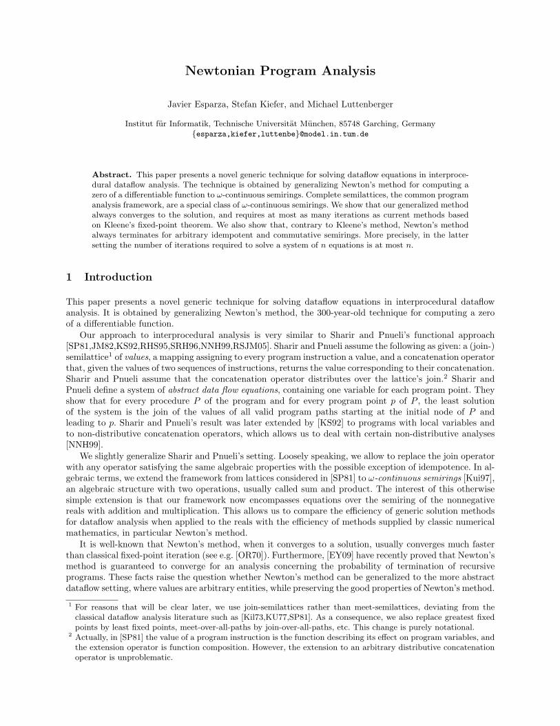
[SP81] show that JOP0 is equal to the least solution of a system of dataflow equations. We sketch how toconstruct the equations by means of an example. Consider a program with three procedures X,Y,Z, whoseflowgraphs are shown in Figure 1. Nodes correspond to program points, and edges to program instructions.For instance, procedure X can execute b and terminate, or execute a, call itself recursively, and, after thecall has terminated, call Y .

n1

n2

n3

n5

n6 n7

n8 n9

n11

n12

n13

n4 n10 n14

X Y Z

a

bcall X

call Y

cd

ecall Y call Y

call Zcall X

g

icall X

h

Fig. 1. Flowgraphs of three procedures

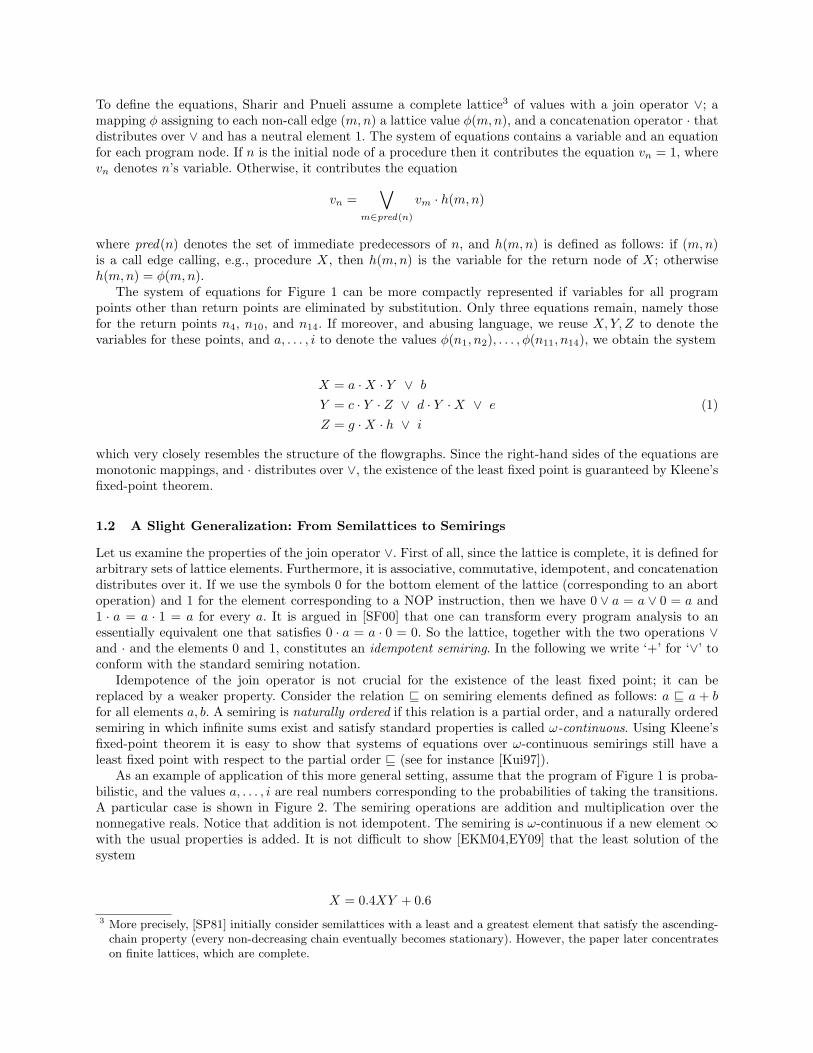
To define the equations, Sharir and Pnueli assume a complete lattice3 of values with a join operator ∨; amapping φ assigning to each non-call edge (m,n) a lattice value φ(m,n), and a concatenation operator · thatdistributes over ∨ and has a neutral element 1. The system of equations contains a variable and an equationfor each program node. If n is the initial node of a procedure then it contributes the equation vn = 1, wherevn denotes n’s variable. Otherwise, it contributes the equation

vn =∨

m∈pred(n)

vm · h(m,n)

where pred(n) denotes the set of immediate predecessors of n, and h(m,n) is defined as follows: if (m,n)is a call edge calling, e.g., procedure X, then h(m,n) is the variable for the return node of X; otherwiseh(m,n) = φ(m,n).

The system of equations for Figure 1 can be more compactly represented if variables for all programpoints other than return points are eliminated by substitution. Only three equations remain, namely thosefor the return points n4, n10, and n14. If moreover, and abusing language, we reuse X,Y,Z to denote thevariables for these points, and a, . . . , i to denote the values φ(n1, n2), . . . , φ(n11, n14), we obtain the system

X = a · X · Y ∨ b

Y = c · Y · Z ∨ d · Y · X ∨ e (1)

Z = g · X · h ∨ i

which very closely resembles the structure of the flowgraphs. Since the right-hand sides of the equations aremonotonic mappings, and · distributes over ∨, the existence of the least fixed point is guaranteed by Kleene’sfixed-point theorem.

1.2 A Slight Generalization: From Semilattices to Semirings

Let us examine the properties of the join operator ∨. First of all, since the lattice is complete, it is defined forarbitrary sets of lattice elements. Furthermore, it is associative, commutative, idempotent, and concatenationdistributes over it. If we use the symbols 0 for the bottom element of the lattice (corresponding to an abortoperation) and 1 for the element corresponding to a NOP instruction, then we have 0 ∨ a = a ∨ 0 = a and1 · a = a · 1 = a for every a. It is argued in [SF00] that one can transform every program analysis to anessentially equivalent one that satisfies 0 · a = a · 0 = 0. So the lattice, together with the two operations ∨and · and the elements 0 and 1, constitutes an idempotent semiring. In the following we write ‘+’ for ‘∨’ toconform with the standard semiring notation.

Idempotence of the join operator is not crucial for the existence of the least fixed point; it can bereplaced by a weaker property. Consider the relation ⊑ on semiring elements defined as follows: a ⊑ a + bfor all elements a, b. A semiring is naturally ordered if this relation is a partial order, and a naturally orderedsemiring in which infinite sums exist and satisfy standard properties is called ω-continuous. Using Kleene’sfixed-point theorem it is easy to show that systems of equations over ω-continuous semirings still have aleast fixed point with respect to the partial order ⊑ (see for instance [Kui97]).

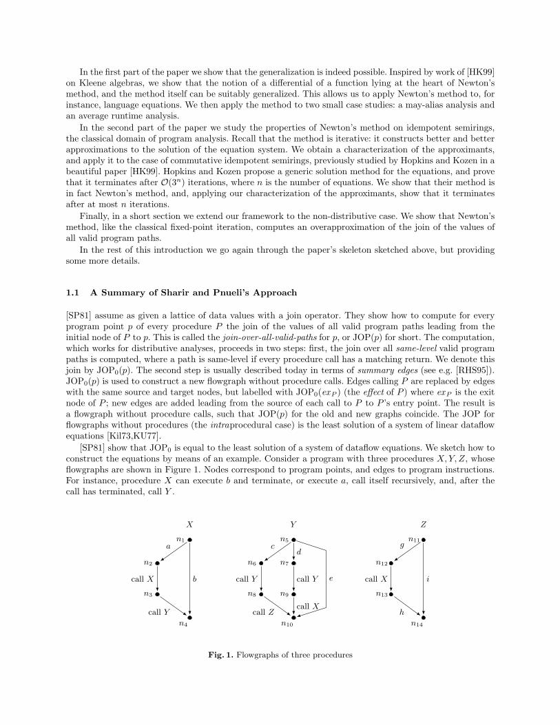
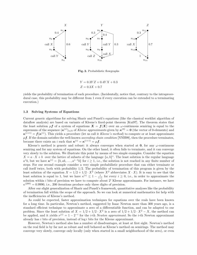
As an example of application of this more general setting, assume that the program of Figure 1 is proba-bilistic, and the values a, . . . , i are real numbers corresponding to the probabilities of taking the transitions.A particular case is shown in Figure 2. The semiring operations are addition and multiplication over thenonnegative reals. Notice that addition is not idempotent. The semiring is ω-continuous if a new element ∞with the usual properties is added. It is not difficult to show [EKM04,EY09] that the least solution of thesystem

X = 0.4XY + 0.6

3 More precisely, [SP81] initially consider semilattices with a least and a greatest element that satisfy the ascending-chain property (every non-decreasing chain eventually becomes stationary). However, the paper later concentrateson finite lattices, which are complete.

n1

n2

n3

n5

n6 n7

n8 n9

n11

n12

n13

n4 n10 n14

X Y Z

0.4

0.6call X

call Y

0.30.4

0.3call Y call Y

call Zcall X

0.3

0.7call X

1

Fig. 2. Probabilistic flowgraphs

Y = 0.3Y Z + 0.4Y X + 0.3

Z = 0.3X + 0.7

yields the probability of termination of each procedure. (Incidentally, notice that, contrary to the intraproce-dural case, this probability may be different from 1 even if every execution can be extended to a terminatingexecution.)

1.3 Solving Systems of Equations

Current generic algorithms for solving Sharir and Pnueli’s equations (like the classical worklist algorithm ofdataflow analysis) are based on variants of Kleene’s fixed-point theorem [Kui97]. The theorem states thatthe least solution µf of a system of equations X = f(X) over an ω-continuous semiring is equal to thesupremum of the sequence (κ(i))i∈N of Kleene approximants given by κ(0) = 0 (the vector of 0-elements) andκ(i+1) = f(κ(i)). This yields a procedure (let us call it Kleene’s method) to compute or at least approximateµf . If the domain satisfies the well-known ascending chain condition [NNH99], then the procedure terminates,because there exists an i such that κ(i) = κ(i+1) = µf .

Kleene’s method is generic and robust: it always converges when started at 0, for any ω-continuoussemiring and for any system of equations. On the other hand, it often fails to terminate, and it can convergevery slowly to the solution. We illustrate this point by means of two simple examples. Consider the equationX = a · X + b over the lattice of subsets of the language {a, b}∗. The least solution is the regular languagea∗b, but we have κ(i) = {b, ab, . . . , ai−1b} for i ≥ 1, i.e., the solution is not reached in any finite number ofsteps. For our second example consider a very simple probabilistic procedure that can either terminate orcall itself twice, both with probability 1/2. The probability of termination of this program is given by theleast solution of the equation X = 1/2 + 1/2 · X2 (where X2 abbreviates X · X). It is easy to see that theleast solution is equal to 1, but we have κ(i) ≤ 1 − 1

i+1 for every i ≥ 0, i.e., in order to approximate the

solution within i bits of precision we have to compute about 2i Kleene approximants. For instance, we haveκ(200) = 0.9990, i.e., 200 iterations produce only three digits of precision.

After our slight generalization of Sharir and Pnueli’s framework, quantitative analyses like the probabilityof termination fall within the scope of the approach. So we can look at numerical mathematics for help withthe inefficiencies of Kleene’s method.

As could be expected, faster approximation techniques for equations over the reals have been knownfor a long time. In particular, Newton’s method, suggested by Isaac Newton more than 300 years ago, is astandard efficient technique to approximate a zero of a differentiable function, and can be adapted to ourproblem. Since the least solution of X = 1/2 + 1/2 · X2 is a zero of 1/2 + 1/2 · X2 − X, the method canbe applied, and it yields ν(i) = 1 − 2−i for the i-th Newton approximant. So the i-th Newton approximantalready has i bits of precision, instead of log i bits for the Kleene approximant.

However, Newton’s method also has a number of disadvantages, at least at first sight. Newton’s methodon the real field is by far not as robust and well behaved as Kleene’s method on semirings. The method mayconverge very slowly, converge only locally (only when started in a small neighborhood of the zero), or even

not converge at all [OR70]. So we face the following situation. Kleene’s method, a robust and general solutiontechnique for arbitrary ω-continuous semirings, is inefficient in many cases. Newton’s method is usually veryefficient, but it is only defined for the real field, and it is not robust.

As part of their study of Recursive Markov Chains, [EY09] showed that a variant of Newton’s methodis robust for certain systems of equations over the real semiring: the method always converges when startedat zero. In other words, moving from the real field to the real semiring (only nonnegative numbers) makesthe instability problems disappear. Inspired by this work, in this paper we obtain a more general result. Weshow that Newton’s method can be generalized to arbitrary ω-continuous semirings, and prove that on thesestructures it is as robust as Kleene’s method. Since lattices, the classical domain of program analysis, arevery close to idempotent semirings, we study in detail Newton’s method in idempotent semirings. We payspecial attention to idempotent semirings with commutative multiplication. Loosely speaking, these semiringscorrespond to counting analysis, in which one is interested in how often program points are visited, but not inwhich order. These semirings do not always satisfy the ascending chain condition, and Kleene’s method maynot terminate. We show that a very elegant iterative solution method for these semirings due to [HK99], isexactly Newton’s method, and always terminates in a finite number of steps. As mentioned above, we furtheruse our characterization of Newton approximants to show that the least fixed point is reached after at mostn iterations, a tight bound, improving on the O(3n) bound of [HK99].

The paper is divided into two parts. The first part introduces our generalization of Newton’s method,and ends with two examples of application to program analysis problems: a may-alias analysis for a programtransforming a tree into a list, and an average runtime analysis for lazy evaluation of And/Or-trees. Thesecond part presents the proofs of our results, investigates Newton’s method in idempotent and commutativesemirings, and extends our approach to semi-distributive program analyses. It is well-known that in this casefixed-point iteration overapproximates the join-over-all-paths value (see e.g. [KS92,RHS95,SRH96,NNH99]).We show that the same property holds for Newton’s method.

The first part of the paper is organized as follows. Section 2 introduces ω-continuous semirings, systemsof fixed-point equations, and some semirings investigated in the rest of the paper. Section 3 recalls Newton’smethod, and generalizes it to arbitrary ω-continuous semirings. Section 4 presents the case studies. Thesecond part starts with Section 5 where we prove the fundamental properties of our generalization, mainlyconvergence to the least fixed point. Section 6 characterizes the Newton approximants in terms of derivationtrees, a generalization of the derivation trees of language theory. Section 7 uses this characterization to provethat for idempotent and commutative semirings Newton’s method always terminates in at most n iterationsfor a system of dimension n. Finally, Section 8 deals with non-distributive program analyses.

2 ω-Continuous Semirings

Definition 2.1. A semiring is a tuple 〈S,+, ·, 0, 1〉 where S is a set containing two distinguished elements0 and 1, and the binary operations +, · : S × S → S satisfy the following conditions:

(1) 〈S,+, 0〉 is a commutative monoid.(2) 〈S, ·, 1〉 is a monoid.(3) 0 · a = a · 0 = 0 for all a ∈ S.(4) a · (b + c) = a · b + a · c and (a + b) · c = a · c + b · c for all a, b, c ∈ S.

A semiring 〈S,+, ·, 0, 1〉 is ω-continuous if the following additional conditions hold:

(5) The relation ⊑ := {(a, b) ∈ S × S | ∃d ∈ S : a + d = b} is a partial order.(6) Every ω-chain (ai)i∈N (i.e. ai ⊑ ai+1 with ai ∈ S) has a supremum w.r.t. ⊑ denoted by supi∈N ai.(7) Given an arbitrary sequence (bi)i∈N, define

∑

i∈N

bi := sup{b0 + b1 + . . . + bi | i ∈ N}

(the supremum exists by condition (6)). For every sequence (ai)i∈N, for every c ∈ S, and for everypartition (Ij)j∈J of N:

c ·(∑

i∈N

ai

)=∑

i∈N

(c · ai),

(∑

i∈N

ai

)· c =

∑

i∈N

(ai · c),∑

j∈J

∑

i∈Ij

aj

=

∑

i∈N

ai .

An (ω-continuous) semiring is idempotent, if a + a = a holds for all a ∈ S. It is commutative, if a · b = b · afor all a, b ∈ S. In an ω-continuous semiring we define the Kleene-star ∗ : S → S by

a∗ :=∑

k∈N

ak = sup{1 + a + a · a + . . . + ak | k ∈ N} for a ∈ S.

For ω-continuous semirings, we have the following important property that addition and multiplication,and subsequently polynomials are ω-continuous, too.

Lemma 2.2. In any ω-continuous semiring 〈S,+, ·, 0, 1〉 addition and multiplication are ω-continuous, i.e.for any ω-chain (ai)i∈N and any c ∈ S we have

c · (supi∈N

ai) = supi∈N

(c · ai), (supi∈N

ai) · c = supi∈N

(ai · c), c + (supi∈N

ai) = supi∈N

(c + ai).

Proof. By (5) and (6) in the definition above, for any ω-chain (ai)i∈N, there exists a sequence (di)i∈N suchthat d0 = a0 and ai +di = ai+1 (i.e. di is a difference of ai+1 and ai), and so supi∈N ai =

∑i∈N

di. The resultfollows by applying (7) to this sequence.

Example 2.3. Common examples of ω-continuous semirings are the real semiring, i.e., nonnegative real num-bers extended by infinity 〈R≥0 ∪{∞},+, ·, 0, 1〉, and the language semiring over some finite alphabet Σ, i.e.,〈2Σ∗

,∪, ·, ∅, {ε}〉 where · stands for the canonical concatenation of languages, and ε for the empty word. Inboth of these instances the natural order coincides with the canonical order on the respective carrier, i.e., inthe real semiring we have ⊑ ≡ ≤, and in the language semiring ⊑ ≡ ⊆.

In the following we often write ab instead of a · b.

2.1 Vectors, Polynomials and Power Series.

Let S be an ω-continuous semiring and let X be a finite set of variables. A vector is a mapping v : X → Swhich assigns every variable X ∈ X the value v(X). We usually write vX for v(X). If there is some naturaltotal order given on X like e.g. the lexicographic order in the case X = {X,Y,Z} or the total order onthe indices in the case X = {X1,X2,X3} we will also write a vector v as a column vector of dimension|X | enumerating the values starting with the lowest variable as the topmost value. The set of all vectors isdenoted by V .

Given a countable set I and a vector vi for every i ∈ I, we denote by∑

i∈I vi the vector given by(∑i∈I vi

)X

=∑

i∈I(vi)X for every X ∈ X . Throughout the paper we use bold letters like ‘v’ or ‘a’ forvectors.

A monomial is a finite expression a1X1a2X2 · · · akXkak+1 , where k ≥ 0, a1, . . . , ak+1 ∈ S andX1, . . . ,Xk ∈ X . Note that this general definition of monomial is necessary as we do not require thatmultiplication is commutative. A polynomial is an expression of the form m1 + . . . + mk where k ≥ 0 andm1, . . . ,mk are monomials. A power series is an expression of the form

∑i∈I mi, where I is a countable set

and mi is a monomial for every i ∈ I.Given a monomial f = a1X1a2X2 . . . akXkak+1 and a vector v, we define f(v), the value of f at v, as

a1vX1a2vX2

· · · akvXkak+1. We extend this to any power series f =

∑i∈I fi by f(v) =

∑i∈I fi(v).

A vector of power series is a mapping f that assigns to each variable X ∈ X a power series f(X). Againwe write fX for f(X). Given a vector v, we define f(v) as the vector satisfying (f(v))X = fX(v) for everyX ∈ X , i.e., f(v) is the vector that assigns to X the result of evaluating the power series fX at v. So, f

naturally induces a mapping f : V → V .

2.2 Fixed-Point Equations and Kleene’s Theorem.

The partial order ⊑ on the semiring S can be lifted to a partial order on vectors, also denoted by ⊑, anddefined by v ⊑ v′ if vX ⊑ v′

X for every X ∈ X .Given a vector of power series f , we are interested in the least fixed point of f , i.e., the least vector v

w.r.t. ⊑ satisfying v = f(v). We briefly recall Kleene’s theorem, which guarantees that the least fixed pointexists.

A mapping f : S → S is monotone if a ⊑ b implies f(a) ⊑ f(b), and ω-continuous if for any infinitechain a0 ⊑ a1 ⊑ a2 ⊑ . . . we have sup{f(ai)} = f(sup{ai}). These definitions are extended to mappingsf : V → V from vectors to vectors by requiring them to hold in every component of f . The following result istaken from [Kui97] and relies on the fact that multiplication and addition are ω-continuous on ω-continuoussemirings, see Lemma 2.2.

Proposition 2.4. Let f be a vector of power series. The mapping induced by f is monotone and ω-continuous. Hence, by Kleene’s theorem, f has a unique least fixed point µf . Further, µf is the supremum(w.r.t. ⊑) of the Kleene sequence given by κ(0) = f(0), and κ(i+1) = f(κ(i)).4

2.3 Some Semiring Interpretations.

We recall that different interesting pieces of information about the program of Figure 1 correspond to the leastsolution of Equations (1) from page 3 over different semirings.5 For the rest of the section let Σ = {a, b, . . . , i}be the set of actions in the program, and let σ denote an arbitrary element of Σ.

Language interpretation Consider the following semiring. The carrier is 2Σ∗

(i.e., the set of languagesover Σ). The semiring element σ is interpreted as the singleton language {σ}. The sum and product operationsare union and concatenation of languages, respectively. We call this structure language semiring over Σ.Under this interpretation, Equations (1) are nothing but the following context-free grammar in Backus-Naurform:

X → aXY | b Y → cY Z | dY X | e Z → gXh | i

The least solution of (1) is the triple (L(X), L(Y ), L(Z)), where, for U ∈ {X,Y,Z}, L(U) denotes the setof terminating executions of the program with U as main procedure, or, in language-theoretic terms, thelanguage of the associated grammar with U as axiom.

Relational interpretation Assume that an action σ corresponds to a program instruction whose semanticsis described by means of a relation Rσ(V, V ′) over a set V of program variables (as usual, primed andunprimed variables correspond to the values before and after executing the instruction). Consider now thefollowing semiring. The carrier is the set of all relations over (V, V ′). The semiring element σ is interpretedas the relation Rσ. The sum and product operations are union and join of relations, respectively, i.e.,(R1 · R2)(V, V ′) = ∃V ′′R1(V, V ′′) ∧ R2(V

′′, V ′). Under this interpretation, the U -component of the leastsolution of (1) is the summary relation RU (V, V ′) containing the pairs V, V ′ such that if procedure U startsat valuation V , then it may terminate at valuation V ′.

Counting interpretation Assume we wish to know how many as, bs, etc. we can observe in a (terminating)execution of the program, but we are not interested in the order in which they occur. In the terminology ofabstract interpretation, we abstract an execution w ∈ Σ∗ by the vector (na, . . . , ni) ∈ N

|Σ| where na, . . . , ni

are the number of occurrences of a, . . . , i in w. We call (na, . . . , ni) the Parikh image of w. The Parikh images

of L(X), L(Y ), L(Z) are the least solution of (1) for the following semiring. The carrier is 2N|Σ|

. The j-thaction of Σ is interpreted as the singleton set {(0, . . . , 0, 1, 0 . . . , 0)} with the “1” at the j-th position. Thesum operation is set union, and the product operation is given by

S · T = {(sa + ta, . . . , si + ti) | (sa, . . . , si) ∈ S, (ta, . . . , ti) ∈ T} .

4 Defining κ(0) = 0 would be more straightforward, but less convenient for this paper.5 This will be no surprise for the reader acquainted with abstract interpretation, but the examples will be used all

throughout the paper.

Probabilistic interpretations Assume that the choices between actions are stochastic. For instance,actions a and b are chosen with probability p and (1−p), respectively. The probability of termination is givenby the least solution of (1) when interpreted over the following semiring (the real semiring) [EKM04,EY09].The carrier is the set of nonnegative real numbers, enriched with an additional element ∞. The semiringelement σ is interpreted as the probability of choosing σ among all enabled actions. Sum and product arethe standard operations on real numbers, suitably extended to ∞.

Assume now that actions are assigned not only a probability, but also a duration. Let dσ denote theduration of σ. We are interested in the expected termination time of the program, under the condition thatthe program terminates (the conditional expected time). For this we consider the following semiring. Theelements are the set of pairs (r1, r2), where r1, r2 are nonnegative reals or ∞. We interpret σ as the pair(pσ, dσ), i.e., the probability and the duration of σ. The sum operation is defined as follows (where to simplifythe notation we use +e and ·e for the operations of the semiring, and + and · for sum and product of reals):

(p1, d1) +e (p2, d2) =

(p1 + p2,

p1 · d1 + p2 · d2

p1 + p2

)

(p1, d1) ·e (p2, d2) = (p1 · p2, d1 + d2)

The reader can easily check that this definition satisfies the semiring axioms. The U -component of the leastsolution of (1) is now the pair (tU , eU ), where tU is the probability that procedure U terminates, and eU isits conditional expected time.

3 Newton’s Method for ω-Continuous Semirings

We introduce our generalization of Newton’s method for ω-continuous semirings. In Section 3.1 we considerthe univariate case, i.e. the case of one equation in a single variable, which already allows us to introduceall important ideas. Here we first recall Newton’s method as known from calculus, i.e., as a method forapproximating a zero of a differentiable function. We then take a close look at the analytical definition,and identify the obstacles for a generalization to ω-continuous semirings. Finally, we propose a definitionthat overcomes the obstacles. In Section 3.2 we turn to the multivariate case and state a fundamentaltheorem which shows that our generalization of Newton’s method is well-defined and converges to the leastfixed point. This lays the foundation to what we call Newtonian program analysis, the application of thegeneralized version of Newton’s method to program analysis. We illustrate the concepts at the end of thissection.

3.1 The Univariate Case

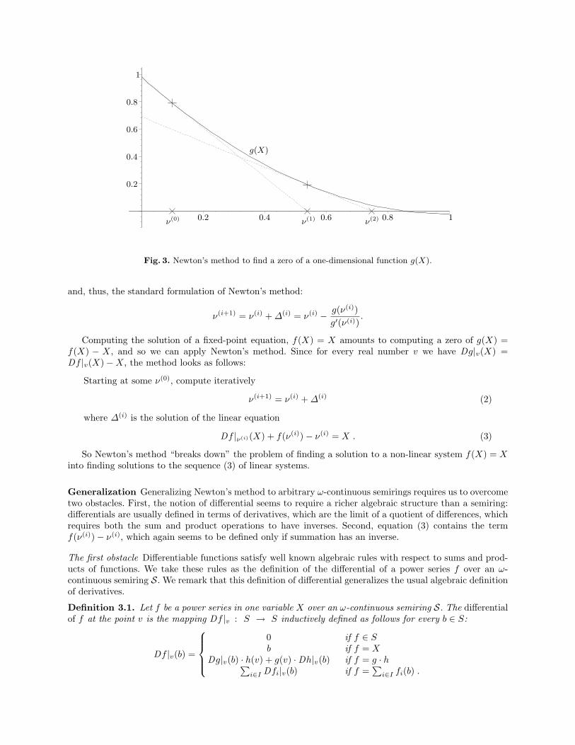
Given a differentiable function g : R → R, Newton’s method computes a zero of g, i.e., a solution of theequation g(X) = 0. The method starts at some value ν(0) “close enough” to the zero, and proceeds iteratively:given ν(i), it computes a value ν(i+1) closer to the zero than ν(i). For that, the method linearizes g at ν(i), i.e.,computes the tangent to g passing through the point (ν(i), g(ν(i))), and takes ν(i+1) as the zero of the tangent(i.e., the x-coordinate of the point at which the tangent cuts the x-axis), see Figure 3 for an illustration.

It is convenient for our purposes to formulate Newton’s method in terms of the differential of g at a givenpoint v ∈ R. Recall that the differential of g is the mapping Dg|v : R → R that assigns to each v ∈ R thelinear function describing the tangent of g at the point (v, g(v)) in the coordinate system having (v, g(v))as origin. If we denote the differential of g at v by Dg|v, then we have Dg|v(X) = g′(v) · X (for example,if g(X) = X2 + 3X + 1, then Dg|3(X) = 9X). In terms of differentials, Newton’s method is formulated asfollows. Starting at some ν(0), compute iteratively ν(i+1) = ν(i) +∆(i), where ∆(i) is the solution of the linearequation Dg|ν(i)(X) + g(ν(i)) = 0 (assume for simplicity that the solution of the linear system is unique). Inparticular for a univariate function g on the real numbers we obtain for ∆(i)

0 = Dg|ν(i)(∆(i)) + g(ν(i)) = g′(ν(i)) · ∆(i) + g(ν(i)), i.e., ∆(i),= − g(ν(i))

g′(ν(i))

0.2

0.2

0.4

0.4

0.6

0.6

0.8

0.8

1

1

ν(0) ν(1) ν(2)

g(X)

Fig. 3. Newton’s method to find a zero of a one-dimensional function g(X).

and, thus, the standard formulation of Newton’s method:

ν(i+1) = ν(i) + ∆(i) = ν(i) − g(ν(i))

g′(ν(i)).

Computing the solution of a fixed-point equation, f(X) = X amounts to computing a zero of g(X) =f(X) − X, and so we can apply Newton’s method. Since for every real number v we have Dg|v(X) =Df |v(X) − X, the method looks as follows:

Starting at some ν(0), compute iteratively

ν(i+1) = ν(i) + ∆(i) (2)

where ∆(i) is the solution of the linear equation

Df |ν(i)(X) + f(ν(i)) − ν(i) = X . (3)

So Newton’s method “breaks down” the problem of finding a solution to a non-linear system f(X) = Xinto finding solutions to the sequence (3) of linear systems.

Generalization Generalizing Newton’s method to arbitrary ω-continuous semirings requires us to overcometwo obstacles. First, the notion of differential seems to require a richer algebraic structure than a semiring:differentials are usually defined in terms of derivatives, which are the limit of a quotient of differences, whichrequires both the sum and product operations to have inverses. Second, equation (3) contains the termf(ν(i)) − ν(i), which again seems to be defined only if summation has an inverse.

The first obstacle Differentiable functions satisfy well known algebraic rules with respect to sums and prod-ucts of functions. We take these rules as the definition of the differential of a power series f over an ω-continuous semiring S. We remark that this definition of differential generalizes the usual algebraic definitionof derivatives.

Definition 3.1. Let f be a power series in one variable X over an ω-continuous semiring S. The differentialof f at the point v is the mapping Df |v : S → S inductively defined as follows for every b ∈ S:

Df |v(b) =

0 if f ∈ Sb if f = X

Dg|v(b) · h(v) + g(v) · Dh|v(b) if f = g · h∑i∈I Dfi|v(b) if f =

∑i∈I fi(b) .

Example 3.2. First consider a polynomial f over some commutative ω-continuous semiring. Because ofcommutative multiplication, we may write any monomial as a · Xk for some k ∈ N and a ∈ S, and sof =

∑nk=0 ak · Xk for suitable n ∈ N and ak ∈ S. Let f ′ denote the usual algebraic derivative of f w.r.t. X,

i.e. f ′ =∑n

k=1 k · ak · Xk−1 where k · ak is an abbreviation of∑k

i=1 ak. We then have

Df |v(b) =∑n

k=0 D(ak · Xk)|v(b)

=∑n

k=0(Dak|v(b) · (Xk)(v) +∑k−1

j=0 ak · (Xj)(v) · DX|v(b) · (Xk−1−j)(v))

=∑n

k=0

∑k−1j=0 ak · vj · DX|v(b) · vk−1−j

= (∑n

k=1 k · ak · vk−1) · b= f ′(v) · b.

So, on commutative semirings, we have Df |v(b) = f ′(v) · b for all v, b ∈ S.

Now, assume that multiplication is not commutative, and consider the simple case of a quadratic mono-mial m = a0Xa1Xa2. We then have

Dm|v(b) = a0 · DX|v(b) · a1 · v · a2 + a0 · v · a1 · DX|v(b) · a2

= a0 · b · a1 · v · a2 + a0 · v · a1 · b · a2.

The important point here is that the differential “remembers” the position of the variables, and thereforedoes not simply append the value b. ⊓⊔

Remark 3.3. Let Σ be a finite alphabet, L ⊆ Σ∗ a language and u ∈ Σ∗ a finite word. In [Brz64] the derivativeDuL of L w.r.t. u is defined to be the language {w | uw ∈ L}. One may relate this notion of derivative toour definition of differential for the special case of univariate power series on idempotent and commutativesemirings. For instance, writing the power series f(X) = a+Xb+XXc as the language Lf := {a,Xb,XXc}(with a, b, c,X ∈ Σ), its derivative w.r.t. X is DXLf = {b,Xc}. Writing this language as power seriesg(X) = b + Xc, we see that g(X) is related to the differential Df by Df |v(e) = be + vce = g(v) · e in thiscase. If multiplication is not commutative, then Df |v(e) = eb + evc + vec, so the equality Df |v(e) = g(v) · eno longer holds.

The second obstacle Profiting from the fact that 0 is the unique minimal element of S with respect to ⊑,we fix ν(0) = f(0), which guarantees ν(0) ⊑ f(ν(0)). We guess that with this choice ν(i) ⊑ f(ν(i)) will holdnot only for i = 0, but for every i ≥ 0 (the correctness of this guess is proved in Theorem 3.9). If the guessis correct, then, by the definition of ⊑, the semiring contains an element δ(i) such that f(ν(i)) = ν(i) + δ(i).We replace f(ν(i)) − ν(i) by any such δ(i). This leads to the following definition:

Definition 3.4. Let f be a power series in one variable. A Newton sequence (ν(i))i∈N is given by:

ν(0) = f(0) and ν(i+1) = ν(i) + ∆(i) (4)

where ∆(i) is the least solution of

Df |ν(i)(X) + δ(i) = X (5)

and δ(i) is any element satisfying f(ν(i)) = ν(i) + δ(i).

Theorem 3.9 below shows that Newton sequences always exist (i.e., there is always at least one possiblechoice for δ(i)), and that they all converge at least as fast as the Kleene sequence. More precisely, we showthat for every i ≥ 0

κ(i) ⊑ ν(i) ⊑ ν(i+1) ⊑ µf .

Since we have µf = supi∈N κ(i) by Kleene’s theorem, Newton sequences converge to µf .

In general, there can be more than one choice for δ(i). But Theorem 3.9 also shows that the Newtonsequence (ν(i))i≥0 itself is uniquely determined by f (and S). In other words, the choice of δ(i) does notinfluence the Newton approximants ν(i).

Let us consider some examples for Newton sequences.

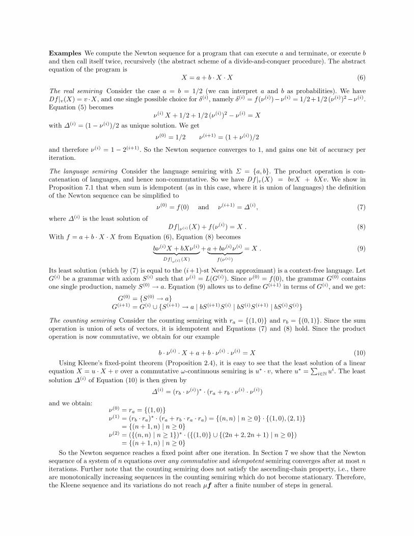
Examples We compute the Newton sequence for a program that can execute a and terminate, or execute band then call itself twice, recursively (the abstract scheme of a divide-and-conquer procedure). The abstractequation of the program is

X = a + b · X · X (6)

The real semiring Consider the case a = b = 1/2 (we can interpret a and b as probabilities). We haveDf |v(X) = v ·X, and one single possible choice for δ(i), namely δ(i) = f(ν(i))−ν(i) = 1/2+1/2 (ν(i))2−ν(i).Equation (5) becomes

ν(i) X + 1/2 + 1/2 (ν(i))2 − ν(i) = X

with ∆(i) = (1 − ν(i))/2 as unique solution. We get

ν(0) = 1/2 ν(i+1) = (1 + ν(i))/2

and therefore ν(i) = 1 − 2(i+1). So the Newton sequence converges to 1, and gains one bit of accuracy periteration.

The language semiring Consider the language semiring with Σ = {a, b}. The product operation is con-catenation of languages, and hence non-commutative. So we have Df |v(X) = bvX + bXv. We show inProposition 7.1 that when sum is idempotent (as in this case, where it is union of languages) the definitionof the Newton sequence can be simplified to

ν(0) = f(0) and ν(i+1) = ∆(i), (7)

where ∆(i) is the least solution ofDf |ν(i)(X) + f(ν(i)) = X . (8)

With f = a + b · X · X from Equation (6), Equation (8) becomes

bν(i)X + bXν(i)

︸ ︷︷ ︸Df |

ν(i) (X)

+ a + bν(i)ν(i)

︸ ︷︷ ︸f(ν(i))

= X . (9)

Its least solution (which by (7) is equal to the (i+1)-st Newton approximant) is a context-free language. LetG(i) be a grammar with axiom S(i) such that ν(i) = L(G(i)). Since ν(0) = f(0), the grammar G(0) containsone single production, namely S(0) → a. Equation (9) allows us to define G(i+1) in terms of G(i), and we get:

G(0) = {S(0) → a}G(i+1) = G(i) ∪ {S(i+1) → a | bS(i+1)S(i) | bS(i)S(i+1) | bS(i)S(i)}

The counting semiring Consider the counting semiring with ra = {(1, 0)} and rb = {(0, 1)}. Since the sumoperation is union of sets of vectors, it is idempotent and Equations (7) and (8) hold. Since the productoperation is now commutative, we obtain for our example

b · ν(i) · X + a + b · ν(i) · ν(i) = X (10)

Using Kleene’s fixed-point theorem (Proposition 2.4), it is easy to see that the least solution of a linearequation X = u · X + v over a commutative ω-continuous semiring is u∗ · v, where u∗ =

∑i∈N

ui. The least

solution ∆(i) of Equation (10) is then given by

∆(i) = (rb · ν(i))∗ · (ra + rb · ν(i) · ν(i))

and we obtain:ν(0) = ra = {(1, 0)}ν(1) = (rb · ra)∗ · (ra + rb · ra · ra) = {(n, n) | n ≥ 0} · {(1, 0), (2, 1)}

= {(n + 1, n) | n ≥ 0}ν(2) = ({(n, n) | n ≥ 1})∗ · ({(1, 0)} ∪ {(2n + 2, 2n + 1) | n ≥ 0})

= {(n + 1, n) | n ≥ 0}So the Newton sequence reaches a fixed point after one iteration. In Section 7 we show that the Newton

sequence of a system of n equations over any commutative and idempotent semiring converges after at most niterations. Further note that the counting semiring does not satisfy the ascending-chain property, i.e., thereare monotonically increasing sequences in the counting semiring which do not become stationary. Therefore,the Kleene sequence and its variations do not reach µf after a finite number of steps in general.

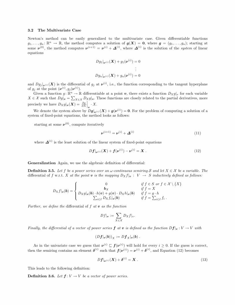
3.2 The Multivariate Case

Newton’s method can be easily generalized to the multivariate case. Given differentiable functionsg1, . . . , gn : R

n → R, the method computes a solution of g(X) = 0, where g = (g1, . . . , gn); starting at

some ν(0), the method computes ν(i+1) = ν(i) + ∆(i), where ∆(i) is the solution of the system of linearequations

Dg1|ν(i)(X) + g1(ν(i)) = 0

...

Dgn|ν(i)(X) + gn(ν(i)) = 0

and Dgj |ν(i)(X) is the differential of gj at ν(i), i.e., the function corresponding to the tangent hyperplaneof gj at the point (ν(i), gj(ν

(i)).Given a function g : R

n → R differentiable at a point v, there exists a function DXg|v for each variableX ∈ X such that Dg|v =

∑X∈X DXg|v. These functions are closely related to the partial derivatives, more

precisely we have DXg|v(X) = ∂g∂X

∣∣∣v· X.

We denote the system above by Dg|ν(i)(X) + g(ν(i)) = 0. For the problem of computing a solution of asystem of fixed-point equations, the method looks as follows:

starting at some ν(0), compute iteratively

ν(i+1) = ν(i) + ∆(i) (11)

where ∆(i) is the least solution of the linear system of fixed-point equations

Df |ν(i)(X) + f(ν(i)) − ν(i) = X . (12)

Generalization Again, we use the algebraic definition of differential:

Definition 3.5. Let f be a power series over an ω-continuous semiring S and let X ∈ X be a variable. Thedifferential of f w.r.t. X at the point v is the mapping DXf |v : V → S inductively defined as follows:

DXf |v(b) =

0 if f ∈ S or f ∈ X \ {X}bX if f = X

DXg|v(b) · h(v) + g(v) · DXh|v(b) if f = g · h∑i∈I DXfi|v(b) if f =

∑i∈I fi .

Further, we define the differential of f at v as the function

Df |v :=∑

X∈XDXf |v.

Finally, the differential of a vector of power series f at v is defined as the function Df |v : V → V with

(Df |v(b))X := DfX |v(b) .

As in the univariate case we guess that ν(i) ⊑ f(ν(i)) will hold for every i ≥ 0. If the guess is correct,

then the semiring contains an element δ(i) such that f(ν(i)) = ν(i) + δ(i), and Equation (12) becomes

Df |ν(i)(X) + δ(i) = X . (13)

This leads to the following definition:

Definition 3.6. Let f : V → V be a vector of power series.

– Let i ∈ N. An i-th Newton approximant ν(i) is inductively defined by

ν(0) = f(0) and ν(i+1) = ν(i) + ∆(i) ,

where ∆(i) is the least solution of Equation (13) and δ(i) is any vector satisfying f(ν(i)) = ν(i) + δ(i).– A sequence (ν(i))i∈N of Newton approximants is called Newton sequence.

Remark 3.7. One can easily show by induction that for any v, b, b′ ∈ V , and any vector of power series f

we haveDf |v(b + b′) = Df |v(b) + Df |v(b′) .

Remark 3.8. If the product operation of the semiring is commutative, the differential DXf |v(a) can bewritten as ∂f

∂X|v · aX , where ∂f

∂X|v denotes the usual partial derivative of the power series f w.r.t. X, taken

at v, as known from algebra:

∂f

∂X

∣∣∣∣v =

0 if f ∈ S or f ∈ X \ {X}1 if f = X

∂g∂x

|v · h(v) + g(v) · ∂h∂X

|v if f = g · h∑i∈I

∂fi

∂X|v if f =

∑i∈I fi .

So, in commutative semirings we may use the usual representation of the differential by means of the gradientof a power series f , or more generally, by the Jacobian of a vector f of power series.

The following fundamental theorem shows that there exists exactly one Newton sequence, that it convergesto the least fixed point, and that it does so at least as fast as the Kleene sequence.

Theorem 3.9. Let f : V → V be a vector of power series.

– There is exactly one Newton sequence (ν(i))i∈N.– The Newton sequence is monotonically increasing, converges to the least fixed point and does so at least

as fast as the Kleene sequence. More precisely, it satisfies

κ(i) ⊑ ν(i) ⊑ f(ν(i)) ⊑ ν(i+1) ⊑ µf = supj∈N

κ(j) for all i ∈ N.

Before giving the formal proof of Theorem 3.9 (see Section 5), we present two examples of Newtonianprogram analysis, which illustrate the use of our generalized Newton’s method to program analysis.

4 Two case studies

We apply our results to the analysis of two small programs. In the first one, a may-alias analysis wherewe use the counting semiring, Kleene iteration does not terminate, while Newton’s method terminates inone step. In the second case, an average runtime analysis where we use the real semiring, neither techniqueterminates, but Newton’s method converges substantially faster to the solution.

4.1 A May-Alias Analysis

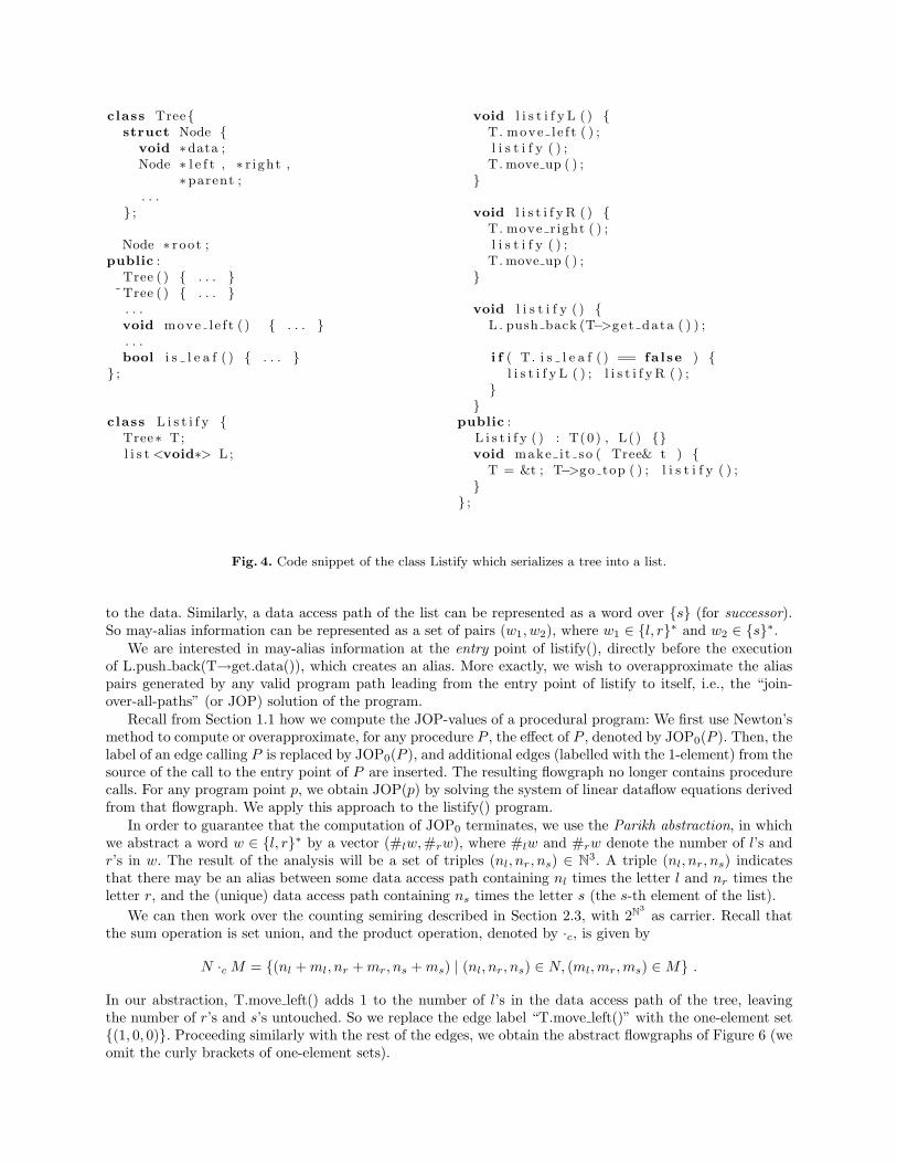
We conduct a may-alias analysis in the spirit of [Deu94]. We consider a program listify() that transforms abinary tree (all non-leaf nodes have two children) of pointers into a list of pointers by reading the nodes ofthe tree in preorder. An implementation in C++ could look as follows, where move right() follows the rightchild pointer, and similarly for move left() and move up().

The flowgraphs of listify(), listifyL(), and listifyR() are shown in Figure 5.We wish to compute may-alias information, i.e., information on which data access paths of the tree and

the list may point to the same element. A data access path of the tree can be represented as a word overthe alphabet {l, r}: for instance, the path llr corresponds to the element found as follows: start at the rootnode, follow twice the pointer to the left child, then once the pointer to the right child, and then the pointer

class Tree{struct Node {

void ∗data ;Node ∗ l e f t , ∗ r i ght ,

∗parent ;. . .

} ;

Node ∗ root ;public :

Tree ( ) { . . . }˜Tree ( ) { . . . }

. . .void move l e f t ( ) { . . . }. . .bool i s l e a f ( ) { . . . }

} ;

class L i s t i f y {Tree∗ T;l i s t <void∗> L ;

void l i s t i f y L ( ) {T. move l e f t ( ) ;l i s t i f y ( ) ;T. move up ( ) ;

}

void l i s t i f y R ( ) {T. move r ight ( ) ;l i s t i f y ( ) ;T. move up ( ) ;

}

void l i s t i f y ( ) {L . push back (T−>get data ( ) ) ;

i f ( T. i s l e a f ( ) == fa l se ) {l i s t i f y L ( ) ; l i s t i f y R ( ) ;

}}

public :L i s t i f y ( ) : T(0 ) , L( ) {}void make i t so ( Tree& t ) {

T = &t ; T−>go top ( ) ; l i s t i f y ( ) ;}

} ;

Fig. 4. Code snippet of the class Listify which serializes a tree into a list.

to the data. Similarly, a data access path of the list can be represented as a word over {s} (for successor).So may-alias information can be represented as a set of pairs (w1, w2), where w1 ∈ {l, r}∗ and w2 ∈ {s}∗.

We are interested in may-alias information at the entry point of listify(), directly before the executionof L.push back(T→get.data()), which creates an alias. More exactly, we wish to overapproximate the aliaspairs generated by any valid program path leading from the entry point of listify to itself, i.e., the “join-over-all-paths” (or JOP) solution of the program.

Recall from Section 1.1 how we compute the JOP-values of a procedural program: We first use Newton’smethod to compute or overapproximate, for any procedure P , the effect of P , denoted by JOP0(P ). Then, thelabel of an edge calling P is replaced by JOP0(P ), and additional edges (labelled with the 1-element) from thesource of the call to the entry point of P are inserted. The resulting flowgraph no longer contains procedurecalls. For any program point p, we obtain JOP(p) by solving the system of linear dataflow equations derivedfrom that flowgraph. We apply this approach to the listify() program.

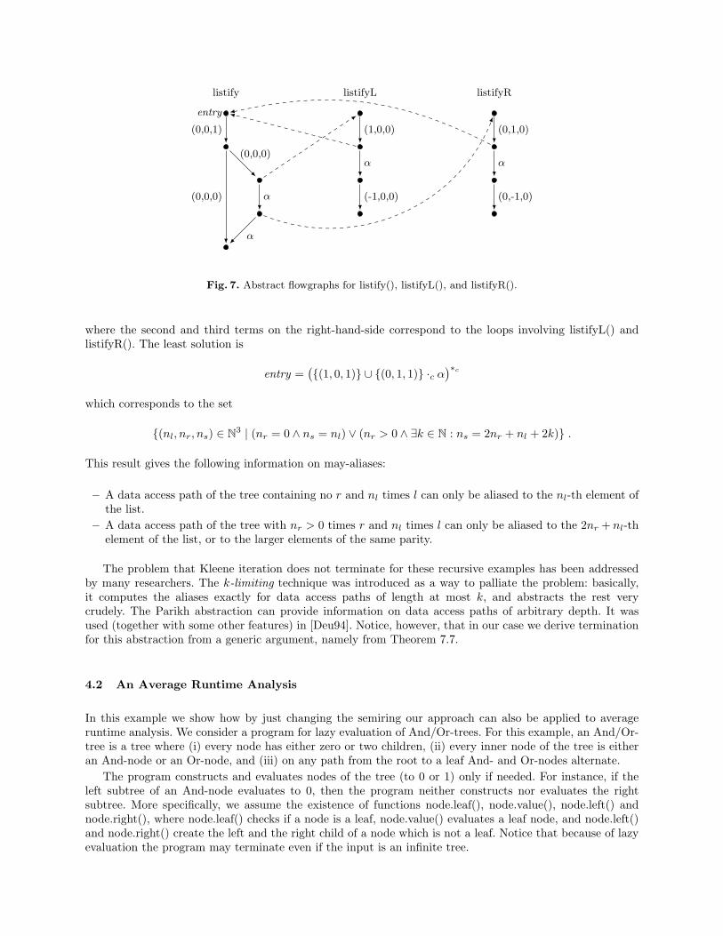
In order to guarantee that the computation of JOP0 terminates, we use the Parikh abstraction, in whichwe abstract a word w ∈ {l, r}∗ by a vector (#lw,#rw), where #lw and #rw denote the number of l’s andr’s in w. The result of the analysis will be a set of triples (nl, nr, ns) ∈ N

3. A triple (nl, nr, ns) indicatesthat there may be an alias between some data access path containing nl times the letter l and nr times theletter r, and the (unique) data access path containing ns times the letter s (the s-th element of the list).

We can then work over the counting semiring described in Section 2.3, with 2N3

as carrier. Recall thatthe sum operation is set union, and the product operation, denoted by ·c, is given by

N ·c M = {(nl + ml, nr + mr, ns + ms) | (nl, nr, ns) ∈ N, (ml,mr,ms) ∈ M} .

In our abstraction, T.move left() adds 1 to the number of l’s in the data access path of the tree, leavingthe number of r’s and s’s untouched. So we replace the edge label “T.move left()” with the one-element set{(1, 0, 0)}. Proceeding similarly with the rest of the edges, we obtain the abstract flowgraphs of Figure 6 (weomit the curly brackets of one-element sets).

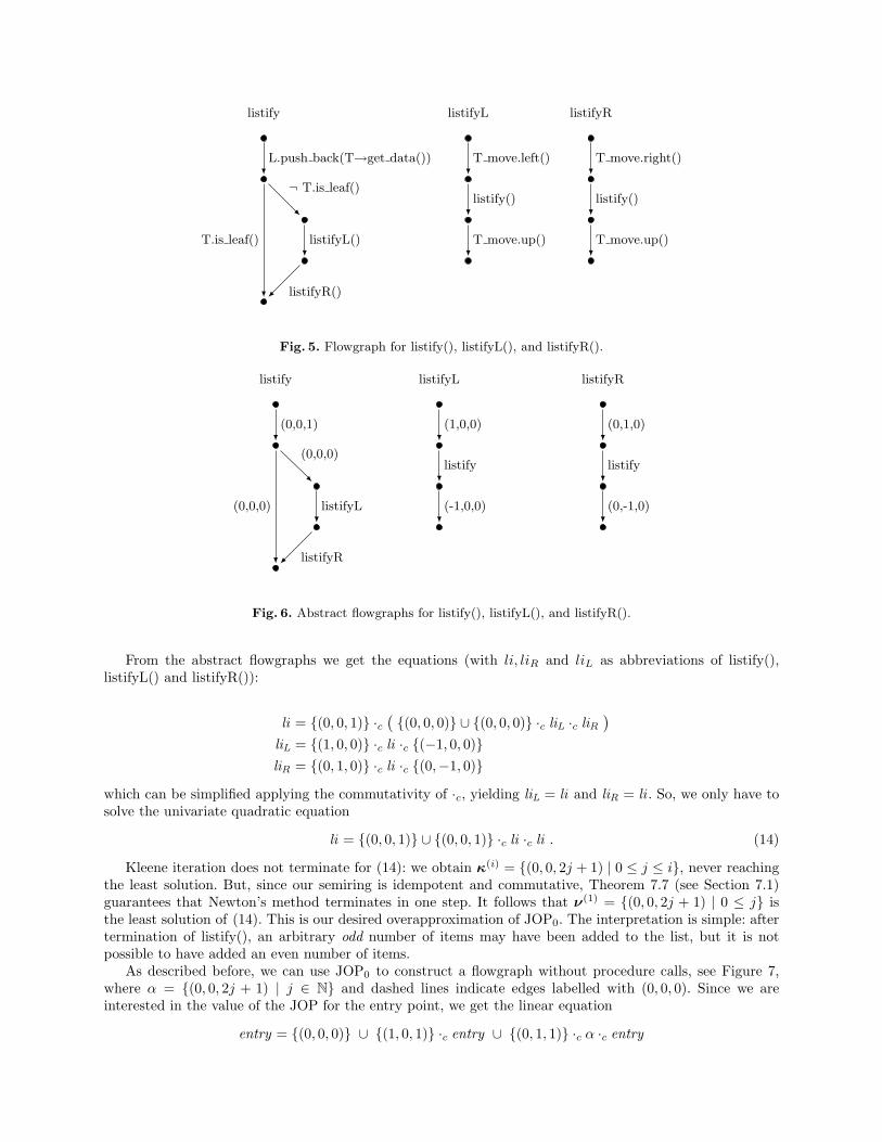
listify

L.push back(T→get data())

T.is leaf()

¬ T.is leaf()

listifyL()

listifyR()

listifyL

T move.left()

listify()

T move.up()

listifyR

T move.right()

listify()

T move.up()

Fig. 5. Flowgraph for listify(), listifyL(), and listifyR().

listify

(0,0,1)

(0,0,0)

(0,0,0)

listifyL

listifyR

listifyL

(1,0,0)

listify

(-1,0,0)

listifyR

(0,1,0)

listify

(0,-1,0)

Fig. 6. Abstract flowgraphs for listify(), listifyL(), and listifyR().

From the abstract flowgraphs we get the equations (with li, liR and liL as abbreviations of listify(),listifyL() and listifyR()):

li = {(0, 0, 1)} ·c({(0, 0, 0)} ∪ {(0, 0, 0)} ·c liL ·c liR

)

liL = {(1, 0, 0)} ·c li ·c {(−1, 0, 0)}liR = {(0, 1, 0)} ·c li ·c {(0,−1, 0)}

which can be simplified applying the commutativity of ·c, yielding liL = li and liR = li . So, we only have tosolve the univariate quadratic equation

li = {(0, 0, 1)} ∪ {(0, 0, 1)} ·c li ·c li . (14)

Kleene iteration does not terminate for (14): we obtain κ(i) = {(0, 0, 2j + 1) | 0 ≤ j ≤ i}, never reachingthe least solution. But, since our semiring is idempotent and commutative, Theorem 7.7 (see Section 7.1)guarantees that Newton’s method terminates in one step. It follows that ν(1) = {(0, 0, 2j + 1) | 0 ≤ j} isthe least solution of (14). This is our desired overapproximation of JOP0. The interpretation is simple: aftertermination of listify(), an arbitrary odd number of items may have been added to the list, but it is notpossible to have added an even number of items.

As described before, we can use JOP0 to construct a flowgraph without procedure calls, see Figure 7,where α = {(0, 0, 2j + 1) | j ∈ N} and dashed lines indicate edges labelled with (0, 0, 0). Since we areinterested in the value of the JOP for the entry point, we get the linear equation

entry = {(0, 0, 0)} ∪ {(1, 0, 1)} ·c entry ∪ {(0, 1, 1)} ·c α ·c entry

listify

entry

(0,0,1)

(0,0,0)

(0,0,0)

α

α

listifyL

(1,0,0)

α

(-1,0,0)

listifyR

(0,1,0)

α

(0,-1,0)

Fig. 7. Abstract flowgraphs for listify(), listifyL(), and listifyR().

where the second and third terms on the right-hand-side correspond to the loops involving listifyL() andlistifyR(). The least solution is

entry =({(1, 0, 1)} ∪ {(0, 1, 1)} ·c α

)∗c

which corresponds to the set

{(nl, nr, ns) ∈ N3 | (nr = 0 ∧ ns = nl) ∨ (nr > 0 ∧ ∃k ∈ N : ns = 2nr + nl + 2k)} .

This result gives the following information on may-aliases:

– A data access path of the tree containing no r and nl times l can only be aliased to the nl-th element ofthe list.

– A data access path of the tree with nr > 0 times r and nl times l can only be aliased to the 2nr + nl-thelement of the list, or to the larger elements of the same parity.

The problem that Kleene iteration does not terminate for these recursive examples has been addressedby many researchers. The k-limiting technique was introduced as a way to palliate the problem: basically,it computes the aliases exactly for data access paths of length at most k, and abstracts the rest verycrudely. The Parikh abstraction can provide information on data access paths of arbitrary depth. It wasused (together with some other features) in [Deu94]. Notice, however, that in our case we derive terminationfor this abstraction from a generic argument, namely from Theorem 7.7.

4.2 An Average Runtime Analysis

In this example we show how by just changing the semiring our approach can also be applied to averageruntime analysis. We consider a program for lazy evaluation of And/Or-trees. For this example, an And/Or-tree is a tree where (i) every node has either zero or two children, (ii) every inner node of the tree is eitheran And-node or an Or-node, and (iii) on any path from the root to a leaf And- and Or-nodes alternate.

The program constructs and evaluates nodes of the tree (to 0 or 1) only if needed. For instance, if theleft subtree of an And-node evaluates to 0, then the program neither constructs nor evaluates the rightsubtree. More specifically, we assume the existence of functions node.leaf(), node.value(), node.left() andnode.right(), where node.leaf() checks if a node is a leaf, node.value() evaluates a leaf node, and node.left()and node.right() create the left and the right child of a node which is not a leaf. Notice that because of lazyevaluation the program may terminate even if the input is an infinite tree.

function And(node)if node.leaf() then

return node.value()else

v := Or(node.left())if v = 0 then

return 0else

return Or(node.right())

function Or(node)if node.leaf() then

return node.value()else

v := And(node.left())if v = 1 then

return 1else

return And(node.right())

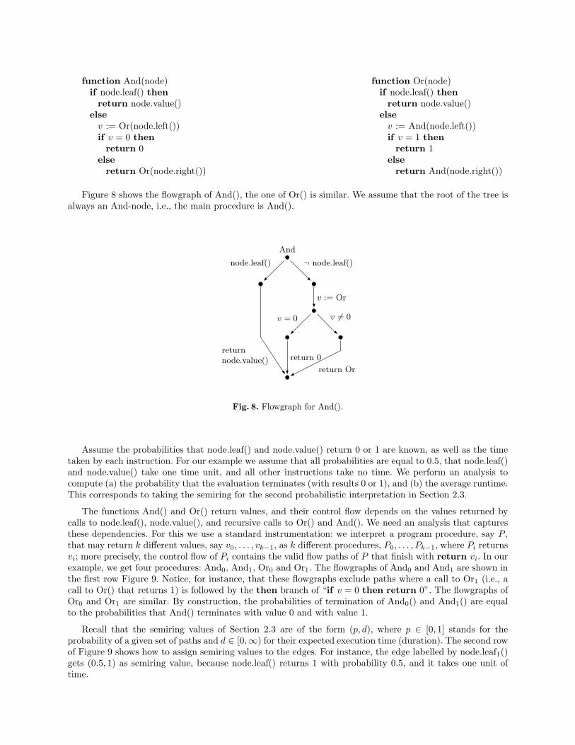
Figure 8 shows the flowgraph of And(), the one of Or() is similar. We assume that the root of the tree isalways an And-node, i.e., the main procedure is And().

And

node.leaf() ¬ node.leaf()

returnnode.value()

v := Or

v = 0 v 6= 0

return 0

return Or

Fig. 8. Flowgraph for And().

Assume the probabilities that node.leaf() and node.value() return 0 or 1 are known, as well as the timetaken by each instruction. For our example we assume that all probabilities are equal to 0.5, that node.leaf()and node.value() take one time unit, and all other instructions take no time. We perform an analysis tocompute (a) the probability that the evaluation terminates (with results 0 or 1), and (b) the average runtime.This corresponds to taking the semiring for the second probabilistic interpretation in Section 2.3.

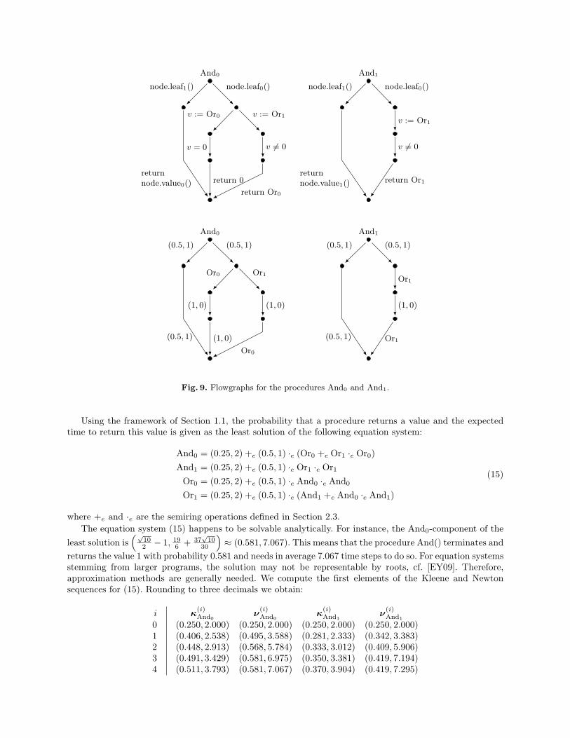
The functions And() and Or() return values, and their control flow depends on the values returned bycalls to node.leaf(), node.value(), and recursive calls to Or() and And(). We need an analysis that capturesthese dependencies. For this we use a standard instrumentation: we interpret a program procedure, say P ,that may return k different values, say v0, . . . , vk−1, as k different procedures, P0, . . . , Pk−1, where Pi returnsvi; more precisely, the control flow of Pi contains the valid flow paths of P that finish with return vi. In ourexample, we get four procedures: And0, And1, Or0 and Or1. The flowgraphs of And0 and And1 are shown inthe first row Figure 9. Notice, for instance, that these flowgraphs exclude paths where a call to Or1 (i.e., acall to Or() that returns 1) is followed by the then branch of “if v = 0 then return 0”. The flowgraphs ofOr0 and Or1 are similar. By construction, the probabilities of termination of And0() and And1() are equalto the probabilities that And() terminates with value 0 and with value 1.

Recall that the semiring values of Section 2.3 are of the form (p, d), where p ∈ [0, 1] stands for theprobability of a given set of paths and d ∈ [0,∞) for their expected execution time (duration). The second rowof Figure 9 shows how to assign semiring values to the edges. For instance, the edge labelled by node.leaf1()gets (0.5, 1) as semiring value, because node.leaf() returns 1 with probability 0.5, and it takes one unit oftime.

And0

node.leaf1() node.leaf0()

returnnode.value0()

v := Or0 v := Or1

v = 0 v 6= 0

return 0

return Or0

And1

node.leaf1() node.leaf0()

returnnode.value1()

v := Or1

v 6= 0

return Or1

And0

(0.5, 1) (0.5, 1)

(0.5, 1)

Or0 Or1

(1, 0) (1, 0)

(1, 0)

Or0

And1

(0.5, 1) (0.5, 1)

(0.5, 1)

Or1

(1, 0)

Or1

Fig. 9. Flowgraphs for the procedures And0 and And1.

Using the framework of Section 1.1, the probability that a procedure returns a value and the expectedtime to return this value is given as the least solution of the following equation system:

And0 = (0.25, 2) +e (0.5, 1) ·e (Or0 +e Or1 ·e Or0)

And1 = (0.25, 2) +e (0.5, 1) ·e Or1 ·e Or1

Or0 = (0.25, 2) +e (0.5, 1) ·e And0 ·e And0

Or1 = (0.25, 2) +e (0.5, 1) ·e (And1 +e And0 ·e And1)

(15)

where +e and ·e are the semiring operations defined in Section 2.3.

The equation system (15) happens to be solvable analytically. For instance, the And0-component of the

least solution is(√

102 − 1, 19

6 + 37√

1030

)≈ (0.581, 7.067). This means that the procedure And() terminates and

returns the value 1 with probability 0.581 and needs in average 7.067 time steps to do so. For equation systemsstemming from larger programs, the solution may not be representable by roots, cf. [EY09]. Therefore,approximation methods are generally needed. We compute the first elements of the Kleene and Newtonsequences for (15). Rounding to three decimals we obtain:

i κ(i)And0

ν(i)And0

κ(i)And1

ν(i)And1

0 (0.250, 2.000) (0.250, 2.000) (0.250, 2.000) (0.250, 2.000)1 (0.406, 2.538) (0.495, 3.588) (0.281, 2.333) (0.342, 3.383)2 (0.448, 2.913) (0.568, 5.784) (0.333, 3.012) (0.409, 5.906)3 (0.491, 3.429) (0.581, 6.975) (0.350, 3.381) (0.419, 7.194)4 (0.511, 3.793) (0.581, 7.067) (0.370, 3.904) (0.419, 7.295)

We have κ(i)Or0

= κ(i)And1

and ν(i)Or0

= ν(i)And1

and similarly for Or1. We observe that the Newton sequence

converges faster than the Kleene sequence. In particular, while the first entry of ν(4)And0

is > 0.58, further

computation shows that i = 21 is the smallest index i such that the first entry of κ(i)And0

is > 0.58.The performance gap between Kleene and Newton iteration can be widened by lowering the leaf proba-

bility from 0.5 to 0.4. In this case, the procedure And() takes, in average, a time of about 29.81 to return thevalue 0; in other words, in this case, the second entry of the And0-component of the least solution of (15) isapproximately 29.81. It takes around 222 Kleene iterations to determine that this value is greater than 29.8,whereas 6 Newton iterations suffice to establish the same fact. Actually, numerical analysis shows that whenthe leaf probability tends to (

√33−5)/2 ≈ 0.372, the average runtime tends to infinity, and the gap between

Newton and Kleene iteration grows unboundedly. However, it should be mentioned that a Newton step ismore expensive in general than a Kleene step, since a Newton step requires solving a linear equation systemof dimension 4. In [KLE07,EKL08] and [EKLBP] we have given a detailed analysis of the convergence speedof Newton’s method applied to (numerical) fixed-point equations. In general, the more precision is required,the better is the performance of Newton’s method compared to Kleene iteration.

5 Proof of Fundamental Properties of the Newton Sequences

In this section we prove Theorem 3.9 which states that there exists exactly one Newton sequence, that itconverges to the least fixed point, and that it does so at least as fast as the Kleene sequence. The proof issplit in two propositions. Proposition 5.6 in Section 5.1 states that there is only one Newton sequence. Thefollowing proposition covers the rest of Theorem 3.9:

Proposition 5.1. Let f : V → V be a vector of power series.

– For every Newton approximant ν(i) there exists a vector δ(i) such that f(ν(i)) = ν(i) + δ(i). So there isat least one Newton sequence.

– Any Newton sequence satisfies κ(i) ⊑ ν(i) ⊑ f(ν(i)) ⊑ ν(i+1) ⊑ µf = supj∈N κ(j) for all i ∈ N.

The proof of Proposition 5.1 is based on two lemmata. The first one, an easy consequence of Kleene’stheorem, provides a closed form for the least solution of a linear system of fixed-point equations in terms ofthe Kleene star operator, defined as follows:

Definition 5.2. Let g : V → V be a monotone map. The map g∗ : V → V is defined as g∗(v) :=∑

i∈Ngi(v),

where g0(v) := v, gi+1(v) := g(gi(v)) for every i ≥ 0. Similarly, we set for all j ∈ N: g≤j :=∑

0≤i≤j gi(v).

The existence of∑

i∈Ngi(v) is guaranteed by the properties of ω-continuous semirings. Observe that

v ⊑ g∗(v) and g∗(v) = v + g(g∗(v)) hold.

Lemma 5.3. Let f : V → V be a vector of power series, and u,v ∈ V . Then the least solution of Df |u(X)+v = X is Df |∗u(v). In particular, a Newton sequence from Definition 3.6 can be equivalently defined by setting

ν(0) = f(0) and ν(i+1) = ν(i) + Df |∗ν(i)(δ

(i)).

Proof. Set g(X) := Df |u(X) + v. The vector g is a power series in every component and thus a monotonemap from V to V . By Kleene’s fixed-point theorem, the least solution of g(X) = X is given by sup{gi(0) |i ∈ N} = sup{Df |≤i

u (v) | i ∈ N} = Df |∗u(v). ⊓⊔

The second lemma, which is interesting by itself, is a generalization of Taylor’s theorem to arbitraryω-continuous semirings.

Lemma 5.4. Let f : V → V be a vector of power series and let u,v be two vectors. We have

f(u) + Df |u(v) ⊑ f(u + v) ⊑ f(u) + Df |u+v(v) .

Proof. It suffices to show those inequalities for each component separately, so let w.l.o.g. f = f : V → S bea power series. We proceed by induction on the construction of f . The base case (where f is a constant)

and the case where f is a sum of polynomials are easy, and so it suffices to consider the case in which f is amonomial. So let

f = g · X · afor a monomial g, a variable X ∈ X and a constant a. We have

f(u) = g(u) · uX · a and Df |u(v) = g(u) · vX · a + Dg|u(v) · uX · a .

By induction we obtain:

f(u + v) = g(u + v) · (uX + vX) · a⊒(g(u) + Dg|u(v)

)· (uX + vX) · a

= g(u) · uX · a + g(u) · vX · a + Dg|u(v) · (uX + vX) · a⊒ f(u) + g(u) · vX · a + Dg|u(v) · uX · a= f(u) + Df |u(v)

and

f(u + v) = g(u + v) · (uX + vX) · a⊑(g(u) + Dg|u+v(v)

)· (uX + vX) · a

= g(u) · uX · a + g(u) · vX · a + Dg|u+v(v) · (uX + vX) · a⊑ f(u) + g(u + v) · vX · a + Dg|u+v(v) · (uX + vX) · a= f(u) + Df |u+v(v) ⊓⊔

We can now proceed to prove Proposition 5.1.

Proof (of Proposition 5.1). First we prove for all i ∈ N that a suitable δ(i) exists and, at the same time, thatthe inequality κ(i) ⊑ ν(i) ⊑ f(ν(i)) holds. We proceed by induction on i. The base case i = 0 is easy. Forthe induction step, let i ≥ 0.

κ(i+1) = f(κ(i)) (definition of κ(i))

⊑ f(ν(i)) (induction: κ(i) ⊑ ν(i))

= ν(i) + δ(i) for some δ(i) (induction)

⊑ ν(i) + Df |∗ν(i)(δ(i)) (v ⊑ g∗(v))

= ν(i+1) (Lemma 5.3)

= ν(i) + δ(i) + Df |ν(i)(Df |∗ν(i)(δ(i))) (g∗(v) = v + g(g∗(v)) )

= f(ν(i)) + Df |ν(i)(Df |∗ν(i)(δ(i))) (definition of δ(i))

⊑ f(ν(i) + Df |∗ν(i)(δ(i))) (Lemma 5.4)

= f(ν(i+1)) (Lemma 5.3)

Since ν(i+1) ⊑ f(ν(i+1)), there exists a δ(i+1) such that ν(i+1) +δ(i+1) ⊑ f(ν(i+1)). Next we prove f(ν(i)) ⊑ν(i+1):

f(ν(i)) = ν(i) + δ(i) (as proved above)

⊑ ν(i) + Df |∗ν(i)(δ(i)) (v ⊑ g∗(v))

= ν(i+1) (Lemma 5.3)

It remains to prove supj∈N κ(j) = µf and ν(i) ⊑ µf for all i. The equation supj∈N κ(j) = µf holds by

Kleene’s theorem (Proposition 2.4). To prove ν(i) ⊑ µf for all i we need a lemma.

Lemma 5.5. Let f(x) ⊒ x. For all d ≥ 0 there exists a vector e(d)(x) such that

fd(x) + e(d)(x) = fd+1(x) and

e(d)(x) ⊒ Df |fd−1(x)(Df |fd−2(x)(. . .Df |x(e(0)(x)) . . .))

⊒ Df |dx(e(0)(x)) .

Proof of the lemma. By induction on d. For d = 0 there is an appropriate e(0)(x) by assumption. Letd ≥ 0.

fd+2(x) = f(fd(x) + e(d)(x)) (induction)

⊒ fd+1(x) + Df |fd(x)(e(d)(x)) (Lemma 5.4)

⊒ fd+1(x) + Df |fd(x)(. . .Df |x(e(0)(x)) . . .) (induction)

Therefore, there exists an e(d+1)(x) ⊒ Df |fd(x)(. . .Df |x(e(0)(x)) . . .). Since Df |y is monotone in y and

x ⊑ f(x) ⊑ f2(x) ⊑ . . ., the second inequality also holds. This completes the proof of the lemma. ⊓⊔Notice that Lemma 5.5 holds for x = ν(i) and e(0)(ν(i)) = δ(i), because we have already shown ν(i) ⊑

f(ν(i)). Now we can prove ν(i) ⊑ µf by induction on i. The case i = 0 is trivial. Let i ≥ 0. We have:

ν(i+1) = ν(i) + Df |∗ν(i)(δ(i)) (Lemma 5.3)

= ν(i) +∑

d∈N

Df |dν(i)(δ(i)) (definition of Df |∗ν(i))

⊑ ν(i) +∑

d∈N

e(d)(ν(i)) (Lemma 5.5)

= supd∈N

fd(ν(i)) (ω-continuity)

⊑ µf (induction:

ν(i) ⊑ f(ν(i)) ⊑ f(f(ν(i))) ⊑ . . . ⊑ µf)

This completes the proof of Proposition 5.1. ⊓⊔

5.1 Uniqueness

In Definition 3.6 the Newton approximant ν(i) is defined in terms of a vector δ(i) satisfying ν(i) + δ(i) =f(ν(i)). In the previous section we have shown that such a vector always exists. However, in a semiring there

there may be multiple such δ(i)’s, and so in principle there could be multiple Newton sequences. We shownow that this is not the case, i.e., there is only one Newton sequence (ν(i))i∈N, independent of the choice of

δ(i):

Proposition 5.6. Let f : V → V be a vector of power series. There is exactly one Newton sequence(ν(i))i∈N.

Theorem 3.9 follows directly by combining Proposition 5.1 and Proposition 5.6. So for Theorem 3.9 it remainsto prove Proposition 5.6, which we do in the rest of this section.

It is convenient for this proof to introduce substitutionals, a notion related to differentials, see Defini-tion 3.5.

Definition 5.7. Let f be a power series over an ω-continuous semiring S and let s ∈ N+. The substitutionalof f w.r.t. s at the point v is the mapping $sf |v : V → S defined as follows:If f is a monomial, i.e., of the form f = a1X1 · · · akXkak+1, then

$sf |v(b) =

{a1vX1

· · · as−1vXs−1asbXs

as+1vXs+1· · · akvXk

ak+1 if 1 ≤ s ≤ k

0 otherwise.

If f is a power series, i.e., of the form f =∑

i∈I fi, then

$sf |v(b) =∑

i∈I

$sfi|v(b).

In words: if f is a monomial with at least s variables then $sf |v(b) is obtained from f by replacing the s-thvariable Xs by bXs

and all other variables by the corresponding component of v. If f is a monomial withless than s variables then $sf |v(b) = 0. If f is a power series then the substitutional of f is the sum of thesubstitutionals of f ’s monomials.

Analogously to differentials, we extend the definition of substitutionals to vectors of power series byapplying the substitution componentwise. Formally, we define the substitutional of a vector of power series f

at v as the function $sf |v : V → V with

($sf |v(b))X := $sfX |v(b) .

Observe that, like the differential (see Remark 3.7), the substitutional is “linear”, i.e., $sf |v(b + b′) =$sf |v(b) + $sf |v(b′).

Notation 1. For any j ∈ N and any sequence s = (s1, . . . sj) ∈ Nj+ we write $sf |v(b) for

$s1f |v($s2

f |v(· · · $sjf |v(b) · · · )), and $sf |v(b) = b if j = 0.

The following facts are immediate from the definitions.

Proposition 5.8. Let f be a monomial. Then

DXf |v(b) =∑

{$sf |v(b) | X is the s-th variable in f} .

Let f be a vector of power series. Then:

1. Df |v(b) =∑

s∈N+$sf |v(b).

2. Df |jv(b) =∑

s∈Nj

+$sf |v(b).

3. For all s ∈ N+ we have f(v) ⊒ $sf |v(v).

Example 5.9. Consider the polynomial f = aXY X + cY . Then

$1f |v(b) = abXvY vX + cbY

$2f |v(b) = avXbY vX

$3f |v(b) = avXvY bX

DXf |v(b) = abXvY vX + avXvY bX

DY f |v(b) = avXbY vX + cbY .

Observe that Df |v(b) = DXf |v(b)+DY f |v(b) = $1f |v(b)+$2f |v(b)+$3f |v(b) and that f(v) = avXvY vX +cvY ⊒ $sf |v(v) holds for all s ∈ N+. ⊓⊔

For the proof of Proposition 5.6 we need the following two lemmata.

Lemma 5.10. Let f be a vector of power series. Let ν + δ = f(ν). Let j ∈ N and (s1, . . . , sj+1) ∈ Nj+1+ .

Then ν + Df |≤jν (δ) ⊒ $(s1,...,sj+1)f |ν(ν).

Proof. By induction on j. For j = 0 we have ν +Df |≤0ν (δ) = ν +δ = f(ν) ⊒ $s1

f |ν(ν) by Proposition 5.8.3.Let j ≥ 0. We have:

ν + Df |≤j+1ν (δ) = ν + Df |≤j

ν (δ) + Df |j+1ν (δ)

⊒ $(s1,...,sj+1)f |ν(ν) + Df |j+1ν (δ) (induction)

⊒ $(s1,...,sj+1)f |ν(ν) + $(s1,...,sj+1)f |ν(δ) (Prop. 5.8.2.)

= $(s1,...,sj+1)f |ν(f(ν)) (ν + δ = f(ν))

⊒ $(s1,...,sj+1)f |ν($sj+2f |ν(ν)) (Prop. 5.8.3.)

= $(s1,...,sj+2)f |ν(ν) ⊓⊔

Lemma 5.11. Let f be a vector of power series. Let ν + δ = ν + δ′ = f(ν). Then ν + Df |∗ν(δ) =ν + Df |∗ν(δ′).

Proof. We show ν + Df |≤jν (δ) = ν + Df |≤j

ν (δ′) for all j ∈ N. Then the lemma follows by ω-continuity. Weproceed by induction on j. The induction base (j = 0) is clear. Let j ≥ 0. We have:

ν + Df |≤j+1ν (δ) = ν + Df |≤j

ν (δ) + Df |j+1ν (δ)

= ν + Df |≤jν (δ′) + Df |j+1

ν (δ) (induction)

= ν + Df |≤jν (δ′)︸ ︷︷ ︸

=:u

+∑

s∈Nj+1+

$sf |ν(δ) (Prop. 5.8.2.)

By Lemma 5.10, we have u ⊒ $sf |ν(ν) for all s ∈ Nj+1+ . In other words, for all s ∈ N

j+1+ there is a u′

such that u = u′ + $sf |ν(ν). Hence, for all s ∈ Nj+1+ , we have u + $sf |ν(δ) = u′ + $sf |ν(ν) + $sf |ν(δ) =

u′ + $sf |ν(f(ν)) = u + $sf |ν(δ′). Therefore, in the above equation, we can replace δ by δ′ due to the“presence” of u:

= ν + Df |≤jν (δ′) +

∑

s∈Nj+1+

$sf |ν(δ′) (as argued above)

= ν + Df |≤jν (δ′) + Df |j+1

ν (δ′) (Prop. 5.8.2.)

= ν + Df |≤j+1ν (δ′) ⊓⊔

Now Proposition 5.6 follows immediately from Lemma 5.11 by a straightforward inductive proof. ⊓⊔

6 Derivation Trees and the Newton Approximants

The proofs of the previous section were purely algebraical. For deeper and stronger results we need thenotion of derivation trees. To this end we reinterpret a system of power-series as a context-free grammar,and assign it a set of derivation trees. We then characterize the Kleene and Newton approximants of thesystem in terms of those trees. This characterization of the Newton approximants will be crucially used inthe rest of this paper.

We assume that the reader is familiar with the notion of derivation tree of a context-free grammar. Recallthat the yield of a derivation tree (obtained by reading the leaves from left to right) is a word generated bythe grammar, and every word generated by the grammar is the yield of one or more derivation trees. In ourreinterpretation the non-terminals will be the variables of the system of power series, and the terminals willbe its coefficients.

We show that the Kleene approximants κ(i) are equal to the sum of the yields of the derivation treeshaving a certain height. Similarly, we show that the Newton approximants ν(i) are equal to the sum of theyields of the trees having a certain dimension, a notion introduced in Definition 6.7 below.

For the rest of the section we fix a vector f of power series over a fixed but arbitrary ω-continuoussemiring. Without loss of generality, we assume that fX =

∑j∈J mX,j holds for every variable X ∈ X , i.e.,

we assume that for all variables the sum is over the same countable set J of indices.Consider the set of ordered trees whose nodes are labelled by pairs (X, j), where X ∈ X and j ∈ J .

Sometimes we identify a tree and its root. In particular, we say that a tree t is labelled by (X, j) if its rootis labelled by (X, j). The mappings λ, λv and λm are defined by λ(t) := (X, j), λv(t) := X, and λm(t) := j.Given a set T of trees, we denote by TX the set of trees t ∈ T such that λv(t) = X.

We define the set of derivation trees of f , and show how to assign to each tree a semiring element called theyield of the tree. For technical reasons our definition differs slightly from the straightforward generalizationof derivation trees for grammars.

Definition 6.1 ((derivation tree, yield)). The derivation trees of f and their yields are inductivelydefined as follows:

– For every monomial mX,j of fX , if no variable occurs in mX,j, then the tree t consisting of one singlenode labelled by (X, j) is a derivation tree of f . Its yield Y (t) is equal to mX,j.

– Let mX,j = a1X1a2X2 . . . akXkak+1 for some k ≥ 1, and let t1, . . . , tk be derivation trees of f such thatλv(ti) = Xi for 1 ≤ i ≤ k. Then the tree t labelled by (X, j) and having t1, . . . , tk as (ordered) childrenis also a derivation tree of f , and its yield Y (t) is equal to a1Y (t1) . . . akY (tk)ak+1.

The yield Y (T ) of a countable set T of derivation trees is defined by Y (T ) =∑

t∈T Y (t). In the following,we mean derivation tree whenever we say tree.

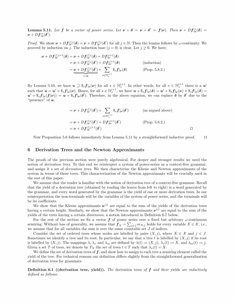
Example 6.2. Figure 10 shows a system of equations (system (1) from the introduction, on the left). Thebasic idea is to read these equations as rules of a context-free grammar, e.g., the equation X = aXY + bis interpreted as the rules X → aXY and X → b. By this reinterpretation derivation trees are naturallyassociated with the given equation system. But as addition is not assumed to be idempotent in general,we have to extend the standard definition of derivation tree in order to handle multiplicities correctly. Thederivation tree depicted in the middle of Figure 10 therefore records which monomial of which variable givesrise to the children of a given node. For instance, consider the node labelled by (Y, 1) (the right child ofthe root). Since the first monomial of the equation for Y is cY Z, the node has two children, say c1, c2 withλv(c1) = Y and λv(c2) = Z. As λm(c2) = 2, the children of c2 are determined by the second monomial ofthe equation for Z. Since this monomial is h, which contains no variables, c2 has no children. The right partof the figure shows the result of labelling each node of the tree with the yield of the subtree rooted at it.

X = aXY + bY = cY Z + dY X + eZ = gXh + i

(X, 1)

(X, 2) (Y, 1)

(Y, 2) (Z, 2)

(Y, 3) (X, 2)

abcdebi

b cdebi

deb i

e b

Fig. 10. A system of equations, a derivation tree, and its yield

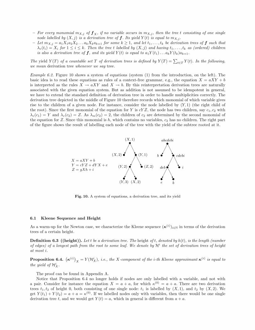
6.1 Kleene Sequence and Height

As a warm-up for the Newton case, we characterize the Kleene sequence (κ(i))i∈N in terms of the derivationtrees of a certain height.

Definition 6.3 ((height)). Let t be a derivation tree. The height of t, denoted by h(t), is the length (numberof edges) of a longest path from the root to some leaf. We denote by Hi the set of derivation trees of heightat most i.

Proposition 6.4.(κ(i)

)X

= Y (HiX), i.e., the X-component of the i-th Kleene approximant κ(i) is equal to

the yield of HiX .

The proof can be found in Appendix A.Notice that Proposition 6.4 no longer holds if nodes are only labelled with a variable, and not with

a pair. Consider for instance the equation X = a + a, for which κ(0) = a + a. There are two derivationtrees t1, t2 of height 0, both consisting of one single node: t1 is labelled by (X, 1), and t2 by (X, 2). Weget Y (t1) + Y (t2) = a + a = κ(0). If we labelled nodes only with variables, then there would be one singlederivation tree t, and we would get Y (t) = a, which in general is different from a + a.

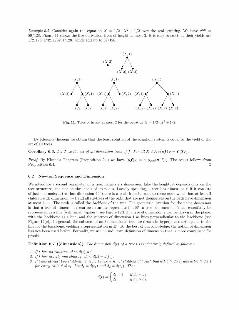
Example 6.5. Consider again the equation X = 1/2 · X2 + 1/2 over the real semiring. We have κ(2) =89/128. Figure 11 shows the five derivation trees of height at most 2. It is easy to see that their yields are1/2, 1/8, 1/32, 1/32, 1/128, which add up to 89/128.

(X, 2)

(X, 1)

(X, 2) (X, 2)

(X, 1)

(X, 2) (X, 1)

(X, 2) (X, 2)

(X, 1)

(X, 1) (X, 2)

(X, 2) (X, 2)

(X, 1)

(X, 1) (X, 1)

(X, 2) (X, 2) (X, 2) (X, 2)

Fig. 11. Trees of height at most 2 for the equation X = 1/2 · X2 + 1/2.

By Kleene’s theorem we obtain that the least solution of the equation system is equal to the yield of theset of all trees.

Corollary 6.6. Let T be the set of all derivation trees of f . For all X ∈ X : (µf)X = Y (TX).

Proof. By Kleene’s Theorem (Proposition 2.4) we have (µf)X = supi∈N(κ(i))X . The result follows fromProposition 6.4. ⊓⊔

6.2 Newton Sequence and Dimension

We introduce a second parameter of a tree, namely its dimension. Like the height, it depends only on thetree structure, and not on the labels of its nodes. Loosely speaking, a tree has dimension 0 if it consistsof just one node; a tree has dimension i if there is a path from its root to some node which has at least 2children with dimension i−1 and all subtrees of the path that are not themselves on the path have dimensionat most i − 1. The path is called the backbone of the tree. The geometric intuition for the name dimensionis that a tree of dimension i can be naturally represented in R

i: a tree of dimension 1 can essentially berepresented as a line (with small “spikes”, see Figure 12(b)); a tree of dimension 2 can be drawn in the plane,with the backbone as a line, and the subtrees of dimension 1 as lines perpendicular to the backbone (seeFigure 12(c)). In general, the subtrees of an i-dimensional tree are drawn in hyperplanes orthogonal to theline for the backbone, yielding a representation in R

i. To the best of our knowledge, the notion of dimensionhas not been used before. Formally, we use an inductive definition of dimension that is more convenient forproofs.

Definition 6.7 ((dimension)). The dimension d(t) of a tree t is inductively defined as follows:

1. If t has no children, then d(t) = 0.2. If t has exactly one child t1, then d(t) = d(t1).3. If t has at least two children, let t1, t2 be two distinct children of t such that d(t1) ≥ d(t2) and d(t2) ≥ d(t′)

for every child t′ 6= t1. Let d1 = d(t1) and d2 = d(t2). Then

d(t) =

{d1 + 1 if d1 = d2

d1 if d1 > d2.

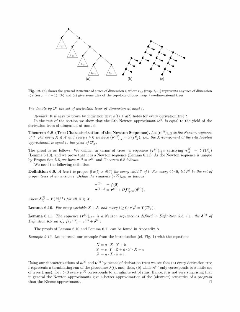
t<i

t<i

t<i

ti−1 ti−1

(a) (b) (c)

Fig. 12. (a) shows the general structure of a tree of dimension i, where t<i (resp. ti−1) represents any tree of dimension< i (resp. = i − 1). (b) and (c) give some idea of the topology of one-, resp. two-dimensional trees.

We denote by Di the set of derivation trees of dimension at most i.

Remark: It is easy to prove by induction that h(t) ≥ d(t) holds for every derivation tree t.In the rest of the section we show that the i-th Newton approximant ν(i) is equal to the yield of the

derivation trees of dimension at most i:

Theorem 6.8 (Tree Characterization of the Newton Sequence). Let (ν(i))i∈N be the Newton sequenceof f . For every X ∈ X and every i ≥ 0 we have

(ν(i)

)X

= Y (DiX), i.e., the X-component of the i-th Newton

approximant is equal to the yield of DiX .

The proof is as follows. We define, in terms of trees, a sequence (τ (i))i∈N satisfying τ(i)X = Y (Di

X)(Lemma 6.10), and we prove that it is a Newton sequence (Lemma 6.11). As the Newton sequence is uniqueby Proposition 5.6, we have τ (i) = ν(i) and Theorem 6.8 follows.

We need the following definition.

Definition 6.9. A tree t is proper if d(t) > d(t′) for every child t′ of t. For every i ≥ 0, let P i be the set ofproper trees of dimension i. Define the sequence (τ (i))i∈N as follows:

τ (0) = f(0)

τ (i+1) = τ (i) + Df |∗τ (i)(δ

(i)) ,

where δ(i)X = Y (P i+1

X ) for all X ∈ X .

Lemma 6.10. For every variable X ∈ X and every i ≥ 0: τ(i)X = Y (Di

X).

Lemma 6.11. The sequence (τ (i))i∈N is a Newton sequence as defined in Definition 3.6, i.e., the δ(i) of

Definition 6.9 satisfy f(τ (i)) = τ (i) + δ(i).

The proofs of Lemma 6.10 and Lemma 6.11 can be found in Appendix A.

Example 6.12. Let us recall our example from the introduction (cf. Fig. 1) with the equations

X = a · X · Y + bY = c · Y · Z + d · Y · X + eZ = g · X · h + i.

Using our characterizations of κ(i) and ν(i) by means of derivation trees we see that (a) every derivation treet represents a terminating run of the procedure λ(t), and, thus, (b) while κ(i) only corresponds to a finite setof trees (runs), for i > 0 every ν(i) corresponds to an infinite set of runs. Hence, it is not very surprising thatin general the Newton approximants give a better approximation of the (abstract) semantics of a programthan the Kleene approximants. ⊓⊔

7 Idempotent Semirings

Recall that in the algebraic structure underlying the framework of [SP81] the summation operator is given bythe join of a semilattice and, thus, summation is idempotent. We therefore study in this section the propertiesof our generalized Newton’s method for this special case of ω-continuous semirings satisfying the additionalaxiom of idempotent addition. We simply call such semirings idempotent ω-continuous semirings, or justidempotent semirings in the following. In idempotent semirings, the natural order can be characterized asfollows: a ⊑ b holds if and only if a + b = b. This is because a ⊑ b means by definition that there is a c suchthat a + c = b. Then we have a + b = a + a + c = a + c = b. This extends analogously to vectors.

We start by showing that in the idempotent case the definition of the Newton sequence (ν(i))i∈N can besimplified.

Proposition 7.1. Let f be a vector of power series over an idempotent semiring. Let (ν(i))i∈N denote theNewton sequence of f . It satisfies the following equations for all i ∈ N:

(a) ν(i+1) = Df |∗ν(i)(f(ν(i)))

(b) ν(i+1) = Df |∗ν(i)(ν

(i))

(c) ν(i+1) = Df |∗ν(i)(f(0))

Proof. We first show (a). By Theorem 3.9 we have ν(i) ⊑ f(ν(i)), hence with idempotence ν(i) + f(ν(i)) =

f(ν(i)). So we can choose δ(i) = f(ν(i)) and have ν(i+1) = ν(i) + Df |∗ν(i)(f(ν(i))) = Df |∗

ν(i)(f(ν(i))),

because ν(i) ⊑ f(ν(i)) ⊑ Df |∗ν(i)(f(ν(i))). So (a) is shown.

Again by Theorem 3.9 we have f(0) = ν(0) ⊑ ν(i) ⊑ f(ν(i)). So we have Df |∗ν(i)(f(0)) ⊑

Df |∗ν(i)(ν

(i)) ⊑ Df |∗ν(i)(f(ν(i))). Hence, for (b) and (c), it remains to show Df |∗

ν(i)(f(ν(i))) ⊑ Df |∗ν(i)(ν

(i))

and Df |∗ν(i)(ν

(i)) ⊑ Df |∗ν(i)(f(0)), respectively. For (b) we have:

Df |∗ν(i)(f(ν(i)))

⊑ Df |∗ν(i)(f(0) + Df |ν(i)(ν(i))) (Lemma 5.4)

= Df |∗ν(i)(f(0)) + Df |∗ν(i)(Df |ν(i)(ν(i)))

⊑ Df |∗ν(i)(ν(i)) + Df |∗ν(i)(Df |ν(i)(ν(i))) (f(0) ⊑ ν(i))

⊑ Df |∗ν(i)(ν(i)) + Df |∗ν(i)(ν

(i)) (Lemma 5.3)

= Df |∗ν(i)(ν(i)) (idempotence)

So (b) is shown.For (c) it remains to show Df |∗

ν(i)(ν(i)) ⊑ Df |∗

ν(i)(f(0)). We proceed by induction on i. The base case

i = 0 is easy because ν(0) = f(0). Let i ≥ 1. We have:

Df |∗ν(i)(ν(i))

= Df |∗ν(i)(Df |∗ν(i−1)(ν(i−1))) (by (b))

⊑ Df |∗ν(i)(Df |∗ν(i−1)(f(0))) (by induction)

⊑ Df |∗ν(i)(Df |∗ν(i)(f(0))) (Theorem 3.9: ν(i−1) ⊑ ν(i))

= Df |∗ν(i)(f(0)) (see explanation below)

For the last step we used that in the idempotent case we have g∗(g∗(x)) = g∗(x) for any linear map g :V → V . Recall that Remark 3.7 states that Df |ν(i) is linear.

g∗(g∗(x)) =∑

j∈N

gj

(∑

k∈N

gk(x)

)(Definition 5.2)

=∑

j∈N

∑

k∈N

gj(gk(x)) (linearity)

=∑

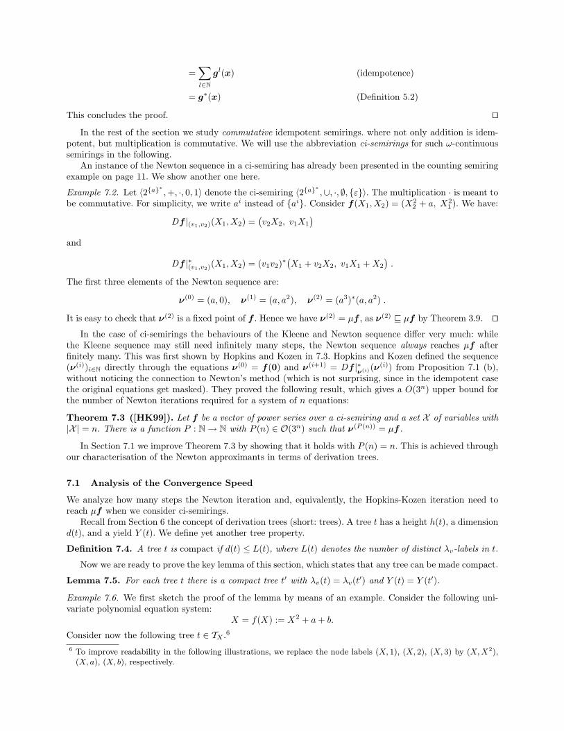
l∈N

gl(x) (idempotence)

= g∗(x) (Definition 5.2)

This concludes the proof. ⊓⊔In the rest of the section we study commutative idempotent semirings. where not only addition is idem-

potent, but multiplication is commutative. We will use the abbreviation ci-semirings for such ω-continuoussemirings in the following.

An instance of the Newton sequence in a ci-semiring has already been presented in the counting semiringexample on page 11. We show another one here.

Example 7.2. Let 〈2{a}∗

,+, ·, 0, 1〉 denote the ci-semiring 〈2{a}∗

,∪, ·, ∅, {ε}〉. The multiplication · is meant tobe commutative. For simplicity, we write ai instead of {ai}. Consider f(X1,X2) = (X2

2 + a, X21 ). We have:

Df |(v1,v2)(X1,X2) =(v2X2, v1X1

)

and

Df |∗(v1,v2)(X1,X2) = (v1v2)

∗(X1 + v2X2, v1X1 + X2

).

The first three elements of the Newton sequence are:

ν(0) = (a, 0), ν(1) = (a, a2), ν(2) = (a3)∗(a, a2) .

It is easy to check that ν(2) is a fixed point of f . Hence we have ν(2) = µf , as ν(2) ⊑ µf by Theorem 3.9. ⊓⊔In the case of ci-semirings the behaviours of the Kleene and Newton sequence differ very much: while

the Kleene sequence may still need infinitely many steps, the Newton sequence always reaches µf afterfinitely many. This was first shown by Hopkins and Kozen in 7.3. Hopkins and Kozen defined the sequence(ν(i))i∈N directly through the equations ν(0) = f(0) and ν(i+1) = Df |∗

ν(i)(ν(i)) from Proposition 7.1 (b),

without noticing the connection to Newton’s method (which is not surprising, since in the idempotent casethe original equations get masked). They proved the following result, which gives a O(3n) upper bound forthe number of Newton iterations required for a system of n equations:

Theorem 7.3 ([HK99]). Let f be a vector of power series over a ci-semiring and a set X of variables with|X | = n. There is a function P : N → N with P (n) ∈ O(3n) such that ν(P (n)) = µf .

In Section 7.1 we improve Theorem 7.3 by showing that it holds with P (n) = n. This is achieved throughour characterisation of the Newton approximants in terms of derivation trees.

7.1 Analysis of the Convergence Speed

We analyze how many steps the Newton iteration and, equivalently, the Hopkins-Kozen iteration need toreach µf when we consider ci-semirings.

Recall from Section 6 the concept of derivation trees (short: trees). A tree t has a height h(t), a dimensiond(t), and a yield Y (t). We define yet another tree property.

Definition 7.4. A tree t is compact if d(t) ≤ L(t), where L(t) denotes the number of distinct λv-labels in t.

Now we are ready to prove the key lemma of this section, which states that any tree can be made compact.

Lemma 7.5. For each tree t there is a compact tree t′ with λv(t) = λv(t′) and Y (t) = Y (t′).

Example 7.6. We first sketch the proof of the lemma by means of an example. Consider the following uni-variate polynomial equation system:

X = f(X) := X2 + a + b.

Consider now the following tree t ∈ TX .6

6 To improve readability in the following illustrations, we replace the node labels (X, 1), (X, 2), (X, 3) by (X, X2),(X, a), (X, b), respectively.

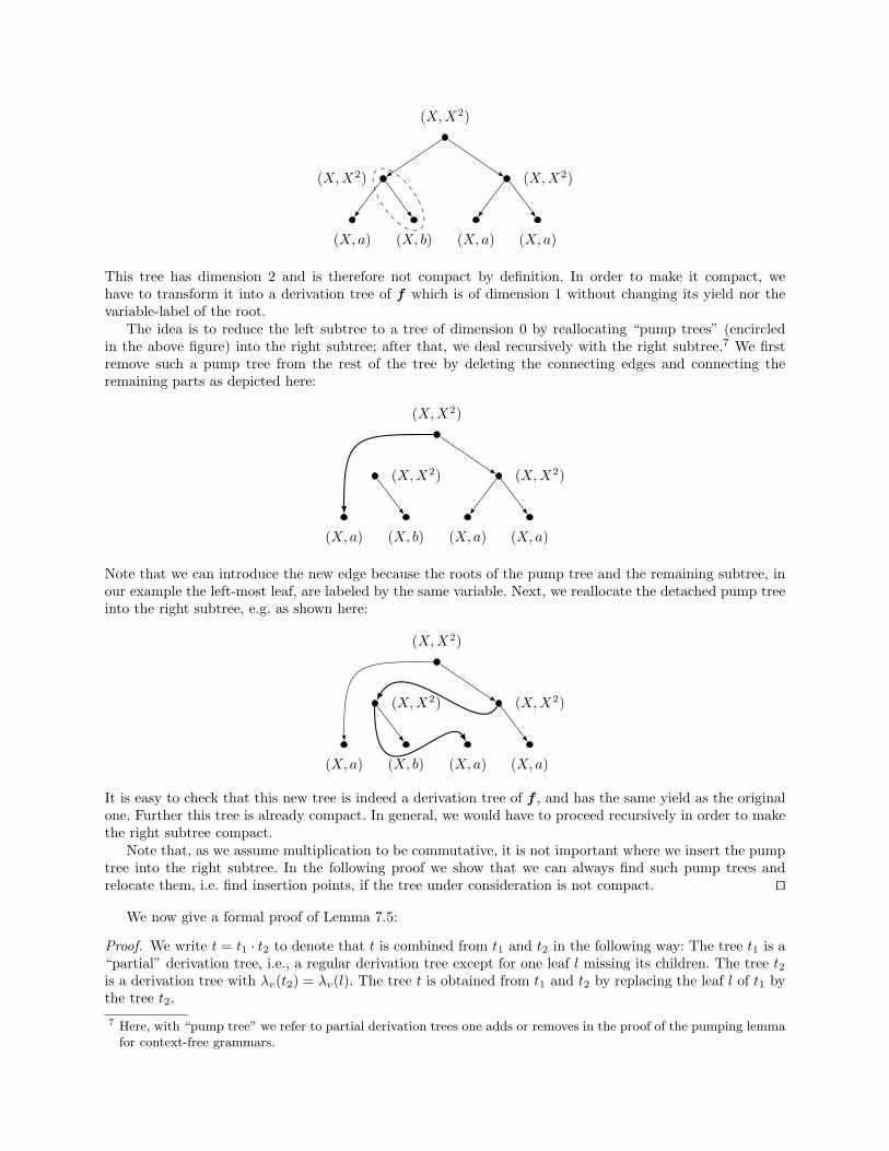
(X,X2)

(X,X2) (X,X2)

(X, a) (X, b) (X, a) (X, a)

This tree has dimension 2 and is therefore not compact by definition. In order to make it compact, wehave to transform it into a derivation tree of f which is of dimension 1 without changing its yield nor thevariable-label of the root.

The idea is to reduce the left subtree to a tree of dimension 0 by reallocating “pump trees” (encircledin the above figure) into the right subtree; after that, we deal recursively with the right subtree.7 We firstremove such a pump tree from the rest of the tree by deleting the connecting edges and connecting theremaining parts as depicted here:

(X,X2)

(X,X2) (X,X2)

(X, a) (X, b) (X, a) (X, a)

Note that we can introduce the new edge because the roots of the pump tree and the remaining subtree, inour example the left-most leaf, are labeled by the same variable. Next, we reallocate the detached pump treeinto the right subtree, e.g. as shown here:

(X,X2)

(X,X2) (X,X2)

(X, a) (X, b) (X, a) (X, a)

It is easy to check that this new tree is indeed a derivation tree of f , and has the same yield as the originalone. Further this tree is already compact. In general, we would have to proceed recursively in order to makethe right subtree compact.

Note that, as we assume multiplication to be commutative, it is not important where we insert the pumptree into the right subtree. In the following proof we show that we can always find such pump trees andrelocate them, i.e. find insertion points, if the tree under consideration is not compact. ⊓⊔

We now give a formal proof of Lemma 7.5:

Proof. We write t = t1 · t2 to denote that t is combined from t1 and t2 in the following way: The tree t1 is a“partial” derivation tree, i.e., a regular derivation tree except for one leaf l missing its children. The tree t2is a derivation tree with λv(t2) = λv(l). The tree t is obtained from t1 and t2 by replacing the leaf l of t1 bythe tree t2.

7 Here, with “pump tree” we refer to partial derivation trees one adds or removes in the proof of the pumping lemmafor context-free grammars.

We proceed by induction on the number of nodes. In the base case, t has just one node, so d(t) = 0,hence t is compact, and we are done. In the following, assume that t has more than one node and d(t) > L(t)holds. We show how to construct a compact tree from t.

Let w.l.o.g. s1, s2, . . . , sr be the children of t with d(t) ≥ d(s1) ≥ d(s2) ≥ . . . ≥ d(sr). By induction wecan make every child compact, i.e. d(si) ≤ L(si). We then have by definition of dimension

L(t) + 1 ≤ d(t) ≤ d(s1) + 1 ≤ L(s1) + 1 ≤ L(t) + 1.

Hence, we have d(t) = d(s1) + 1 which, by definition of dimension and compactness, implies d(s1) = d(s2) =L(t) = L(s1) = L(s2). As h(s2) ≥ d(s2) = L(s2) by the remark after Definition 6.7, we find a path in s2

from the root to a leaf which passes through at least two nodes with the same λv-label, say Xj . In otherwords, we may factor s2 into tb1 · (tb2 · tb3) such that λv(tb2) = λv(t

b3) = Xj . As L(t) = L(s1) = L(s2), we also

find a node of s1 labelled by Xj which allows us to write s1 = ta1 · ta2 with λv(ta2) = Xj .Now we move the middle part of s2 to s1, i.e., let s′1 = ta1 · (tb2 · ta3) and let s′2 = tb1 · tb3. We then have

L(s′1) = L(s1) = L(s2) ≥ L(s′2). By induction, s′1 and s′2 can be made compact, so d(s′1) ≤ d(s1) = d(s2) ≥d(s′2). Consider the tree t′ obtained from t by replacing s1 by s′1 and s2 by s′2. By commutativity, t and t′

have the same yield. If d(s′2) < d(s2) then d(t′) ≤ d(t) − 1 = L(t) = L(t′) and we are done. Otherwise weiterate the described procedure.

This procedure terminates, because the number of nodes of (the current) s2 strictly decreases in everyiteration, and the number of nodes is an upper bound for h(s2) and, therefore, for d(s2). ⊓⊔

Now we can prove the main theorem of this section.

Theorem 7.7. Let f be a vector of power series over a ci-semiring S given in the set X of variables with|X | = n. Then ν(n) = µf .

Proof. We have for all X ∈ X :

(µf)X =∑

trees t with λv(t)=X

Y (t) (Corollary 6.6)

=∑

trees t with λv(t)=X

and d(t)≤n

Y (t) (Lemma 7.5)

= (ν(n))X (Theorem 6.8) ⊓⊔

Remark 7.8. The bound of this theorem is tight, as shown by the following example: If f(X1, . . . ,Xn) =(X2

2 + a,X23 , . . . ,X2

n,X21 ), then (ν(k))X1

= a for k < n, but a2n ≤ (ν(n))X1= (µf)X1

.

8 Non-Distributive Program Analyses

In this paper we have focused on distributive program analyses, which allows us to use semirings as algebraicstructure. Recall that semirings are distributive, i.e., all semiring elements a, b, c satisfy a · (b+c) = a ·b+a ·cand (a + b) · c = a · c + b · c.

Distributive intraprocedural analyses (i.e., for programs without procedures) were considered first in[Kil73]. This seminal paper showed that, given a program and the distributive transfer functions of a programanalysis, one can construct a vector f of polynomials such that, for every program point p, the p-componentof the least fixed point µf coincides with the JOP0-value, i.e., the join over all valid paths where for everyprocedure call there is a matching return (as described in the introduction 1.1).

The framework of [Kil73] was generalized to non-distributive transfer functions in [KU77]. Non-distributivity means, in our terms, that only subdistributivity holds: a · (b + c) ⊒ a · b + a · c and(a + b) · c ⊒ a · c + b · c.8 There are interesting program analyses, such as constant propagation, which

8 If addition is idempotent (as for lattice joins) this condition is equivalent to the monotonicity of multiplication, or,in traditional terms, to the monotonicity of the transfer functions [KU77]. The stricter distributivity condition, onthe other hand, amounts to requiring the transfer functions to be homomorphisms.

are non-distributive, see e.g. [KU77,NNH99]. In those cases, the least fixed point does not necessarily coin-cide with the JOP0-value, but rather safely approximates (“overapproximates”) it.

[SP81] extended the work of [Kil73] to the interprocedural case. The generalization to non-distributiveanalyses was done by [KS92], who proved that, as in the intraprocedural case, the least fixed point is anoverapproximation of the JOP0-value.

We define the JOP0-value as the vector M with Mp = Y (Tp), where Tp is the set of trees labeled with p.Notice that a depth-first traversal of a tree labeled with p precisely corresponds to an interprocedural pathfrom the beginning of the procedure of p to the program point p, i.e., the JOP0-value Mp = Y (Tp) is indeedthe sum of the dataflow values of all paths to p. Corollary 6.6 states that M = µf holds in the distributivecase. Proposition 2.4 and Theorem 3.9 show that the Kleene and Newton sequences converge to this value.

For the non-distributive case, the least fixed point overapproximates the JOP0-value, i.e., M ⊑ µf , cf.[KS92].

In the following we show that Newton’s method is still well-defined in “sub-distributive semirings”, andthat the Kleene and Newton sequences both converge to overapproximations of M , more precisely, we showM ⊑ supi∈N κ(i) ⊑ supi∈N ν(i).

For this we first define subdistributive (ω-complete) semirings9:

Definition 8.1. A subdistributive semiring is a tuple 〈S,+, ·, 0, 1〉 satisfying the following properties:

1. 〈S,+, 0〉 is a commutative monoid.2. 〈S, ·, 1〉 is a monoid.3. 0 · a = a · 0 = 0 for all a ∈ S.4. a · (b + c) ⊒ a · b + a · c and (a + b) · c ⊒ a · c + b · c for all a, b, c ∈ S.5. The relation ⊑ := {(a, b) ∈ S × S | ∃d ∈ S : a + d = b} is a partial order.

6. For all ω-chains (ai)i∈N (i.e. a0 ⊑ a1 ⊑ a2 ⊑ . . . with ai ∈ S) sup⊑i∈N

ai exists. For any sequence (bi)i∈N

define∑

i∈Nbi := sup⊑{b0 + b1 + . . . + bi | i ∈ N}.

Remark 8.2. We obtain the definition of subdistributive semiring from the definition of ω-continuous semiringby removing (7), and replacing distributivity with subdistributivity (see (4)).

In the rest of the section 〈S,+, ·, 0, 1〉 denotes a subdistributive semiring. Polynomials, vectors, differential,etc. are defined as in the distributive setting.

Note that the following inequalities still hold for all sequences (ai)i∈N, c ∈ S, and partitions (Ij)j∈J of N:

c ·(∑

i∈N

ai

)⊒∑

i∈N

(c · ai),

(∑

i∈N

ai

)· c ⊒

∑

i∈N

(ai · c),∑

j∈J

∑

i∈Ij

aj

⊒

∑

i∈N

ai .

Thus, any polynomial p is still monotone, although not necessarily ω-continuous. For any sequence (vi)i∈N

(of vectors) we still have p(∑

i∈Nvi) ⊒ ∑

i∈Np(vi). Hence, the Kleene sequence of a polynomial system f

still converges, but not necessarily to the least fixed point of f :

Corollary 8.3. For any system f of polynomials, the Kleene sequence (κ(i))i∈N is an ω-chain. Moreover,if f has a least solution µf , then supi∈N κ(i) ⊑ µf .

Since the Kleene sequence is still an ω-chain, its limit exists and is a safe approximation of the JOP0-value:

Proposition 8.4. For any polynomial system f we have(κ(i)

)X

⊒ Y (HiX), and, hence,

(supi∈N κ(i)

)X

⊒Y (TX) where TX is the set of trees labeled with X.

We skip the proof of this proposition as it is almost identical to the one of Proposition 6.4. The only differenceis that when expanding the components of κ(i) into a sum of products of coefficients, subdistributivity onlyguarantees that κ(i) is an upper bound, but not equality anymore. Similarly, subdistributivity only allowsus to generalize the lower bound from Lemma 5.4, i.e. we have

f(u) + Df |u(v) ⊑ f(u + v)

for a polynomial system f and vectors u,v.We now turn to the definition of Newton sequence.

9 We drop ω-complete in the following.

Definition 8.5. For f a polynomial system in the variables X, and a, b vectors we set

Lf ;a;b(X) := b + Df |a(X).

Definition 8.6. Let f be a polynomial system.

– Let i ∈ N. An i-th Newton approximant ν(i) is inductively defined by

ν(0) = f(0) and ν(i+1) = ν(i) + ∆(i) ,

where ∆(i) has to satisfy∑

k∈NDf |k

ν(i)(δ(i)) ⊑ ∆(i) ⊑ Lf ;ν(i);δ(i)

(∆(i)

).

– Any such sequence (ν(i))i∈N of Newton approximants is called Newton sequence.

Remark 8.7. If δ(i) exists, then possible choices for ∆(i) are

∑

k∈N

Df |kν(i)(δ(i)), sup

k∈N

Lkf ;ν(i);δ(i)(0) or (if it exists) µLf ;ν(i);δ(i) .

Note that in the distributive setting all three values coincide.

Proposition 8.8. Let f : V → V be a vector of power series.

– For every Newton approximant ν(i) there exists a vector δ(i) such that f(ν(i)) = ν(i) + δ(i). So there isat least one Newton sequence.

– Every Newton sequence ν(i) satisfies κ(i) ⊑ ν(i) ⊑ f(ν(i)) ⊑ ν(i+1) for all i ∈ N.

Proof. First we prove for all i ∈ N that a suitable δ(i) exists and, at the same time, that the inequalityκ(i) ⊑ ν(i) ⊑ f(ν(i)) holds. We proceed by induction on i. For the base case i = 0 we have:

ν(0) = f(0) = κ(0) ⊑ κ(1) = f(κ(0)) = f(ν(0)).

So, there exists a δ(0) with ν(0) + δ(0) = f(ν(0)), and hence we have:

ν(1) = ν(0) + ∆(0) ⊒ ν(0) +∑

k∈N

Df |kν(0)(δ(0)) ⊒ ν(0) + δ(0) = f(ν(0)).

For the induction step, let i ≥ 0.

κ(i+1) = f(κ(i)) ⊑ f(ν(i)) = ν(i) + δ(i) ⊑ ν(i) +∑

k∈N

Df |kν(i)(δ(i)).

As we require that∑

k∈NDf |k

ν(i)(δ(i)) ⊑ ∆(i), it now immediately follows that

κ(i+1) ⊑ ν(i) + ∆(i) = ν(i+1).

By definition of ∆(i) we have ∆(i) ⊑ Lf ;ν(i);δ(i)(∆(i)), it therefore follows:

ν(i+1) = ν(i) + ∆(i) ⊑ ν(i) + δ(i) + Df |ν(i)

(∆(i)

)

= f(ν(i)) + Df |ν(i)

(∆(i)

)⊑ f

(ν(i) + ∆(i)

)= f(ν(i+1)).

We complete our proof by

f(ν(i+1)) = ν(i+1) + δ(i+1) ⊑ ν(i+1) +∑

k∈N

Df |kν(i+1)(δ(i+1))

⊑ ν(i+1) + ∆(i+1) = ν(i+2).

Proposition 8.9. Let M be the JOP0-value, i.e., the vector M with MX = Y (TX). Then M ⊑supi∈N κ(i) ⊑ supi∈N ν(i).

Proof. Follows directly from Propositions 8.4 and 8.8. ⊓⊔

Proposition 8.10. For ∆(i) =∑

k∈NDf |k

ν(i)(δ(i)) we have supi∈N ν(i) ⊑ µf , if µf exists.

Proof. The proof is almost identical to the one of Proposition 5.1. Note that the proof of Lemma 5.5 doesnot use distributivity.

Theorem 8.11 (Tree Characterization of the Newton Sequence). Let (ν(i))i∈N be a Newton sequenceof f . For every X ∈ X and every i ≥ 0 we have

(ν(i)

)X

⊒ Y (DiX), i.e., the X-component of the i-th Newton

approximant is a safe approximation of the yield of DiX .

Proof. In the distributive setting we proved this theorem via induction where we expanded the the termswe obtained using distributivity. In the subdistributive case the same proof still guarantees that

(ν(i)

)X

⊒Y (Di

X).

9 Conclusions

Since its inception, the theory of program analysis has been based on two fundamental observations:

– Analysis problems can be reduced (using abstract interpretation [CC77]) to the mathematical problemof computing the least solution of a system of equations over a semilattice.

– Such systems of equations can be solved using Kleene’s fixed-point theorem as basic algorithm scheme.

In this paper we have contributed to both of these points. On the one hand, we generalize the algebraic settingfrom semilattices to arbitrary semirings (a generalization to idempotent semirings was already present in thework of [RSJM05] on pushdown systems for program analysis). On the other hand, we obtain a new methodfor solving the dataflow equations by generalizing Newton’s method to semirings.

The conceptually simple step from semilattices to semirings leads to a common algebraic setting for“qualitative” analyses (which, loosely speaking, explore the existence of execution paths satisfying a givenproperty) and “quantitative” analyses (in which paths are assigned a numerical weight, and one is interestedin the sum of the weights of all paths satisfying the property). Classical examples of qualitative analyses arelive variables, constant propagation, or alias analysis, while examples of quantitative analysis arise in thestudy of probabilistic programs: probability of termination, expected execution time or, in the interproceduralcase, expected stack height (for the latter, see [EKM05,BEK05]). The common setting allows us to comparethe algorithmic schemes used in the qualitative and quantitative case, and examine if a transfer of techniquesis possible. We have shown that Newton’s method can be generalized to the abstract setting. In particular,it can be applied to qualitative analysis problems.

We have explored Newton’s method for idempotent semirings, i.e., for the semirings corresponding toqualitative analyses. We have shown that the beautiful algebraic algorithm of [HK99] for solving systemsof equations over commutative Kleene algebras is a particular instance of Newton’s method. Moreover, wehave proved that the algorithm requires at most n iterations for a system of n equations, a tight boundthat improves on the O(3n) bound presented in [HK99]. From a theoretical point of view, giving a purelyalgebraic proof of this fact along the lines of [HK99,AEI01] is an interesting challenge.

While this paper imports notions of calculus and numerical mathematics into program analysis, our workalso has some consequences pointing in the opposite direction. Quantitative analyses lead to systems of equa-tions over the real semiring, a particular case of the systems over the real field. Surprisingly, the performanceof Newton’s method in this special case seems not to have received much attention from numerical mathe-maticians. The method turns out to have much better properties than in the general case. A consequenceof our main result (which was already proved, in a slightly more restricted form, by [EY09]), is that on thereal semiring Newton’s method always converges to the least fixed point starting from zero. This is not so inthe real field, where it may not converge or converge only locally, i.e., when started sufficiently close to thezero (see e.g. [Ort72,OR70]). In related work we have shown that the convergence order of the method is atleast linear, meaning that the number of accurate bits of the Newton approximants grows at least linearlywith the number of iterations [KLE07,EKL08,EKLBP].

APPENDIX

A Proofs of Section 6

To avoid typographical clutter in the following proofs, we use the following notation. Given some class ofobjects (e.g. derivation trees t) and a predicate P (t), we write

∑

t

Y (t) : P (t)

instead of ∑

t such that P (t) holds

Y (t) .

Proposition 6.4.(κ(i)

)X

= Y (HiX), i.e., the X-component of the i-th Kleene approximant κ(i) is equal

to the yield of HiX .

Proof. By induction on i. The base case i = 0 is easy. Induction step (i ≥ 0):

(κ(i+1)

)X

= fX(κ(i))

=∑

j∈J

mX,j(κ(i))

=∑

j∈J

y :

{mX,j = a1X1 · · ·Xkak+1

y = a1κ(i)X1

· · ·κ(i)Xk

ak+1

by induction:

=∑

j∈J

y :

{mX,j = a1X1 · · ·Xkak+1

y = a1Y (HiX1

) · · ·Y (HiXk

)ak+1

=∑

j∈J

t1,...,tk

y :

mX,j = a1X1 · · ·Xkak+1

t1, . . . , tk trees with h(tr) ≤ i, λv(tr) = Xr (1 ≤ r ≤ k)y = a1Y (t1) · · ·Y (tk)ak+1

=∑

j∈J,t

Y (t) : t is a tree with h(t) ≤ i + 1, λ(t) = (X, j)

= Y (HiX) ⊓⊔

The following definition of fine dimension is analogous to Definition 6.7, but adds a second component,which measures the length of the path from the root to the lowest node with the same dimension as the root:

Definition A.1 ((fine dimension)). The fine dimension dl(t) = (d(t), l(t)) of a tree t is inductively definedas follows:

1. If t has no children, then dl(t) = (0, 0).2. If t has exactly one child t1, then dl(t) = (d(t1), l(t1) + 1).3. If t has at least two children, let t1, t2 be two distinct children of t such that d(t1) ≥ d(t2) and d(t2) ≥ d(t′)

for every child t′ 6= t1. Let d1 = d(t1) and d2 = d(t2). Then

dl(t) =

{(d1 + 1, 0) if d1 = d2

(d1, l(t1) + 1) if d1 > d2.

Remark A.2. Notice that, by Definition 6.9, a tree t is proper if and only if l(t) = 0. So we have:

Y (P iX) =

∑

t

Y (t) : t tree with λv(t) = X, dl(t) = (i, 0)

Now we can prove the remaining lemmata from Section 6.

Lemma 6.10. For every variable X ∈ X and every i ≥ 0: τ(i)X = Y (Di

X).

Proof. By induction on i. Induction base (i = 0):

τ(0)X = fX(0) =

∑

t

Y (t) : λv(t) = X,h(t) = 0

=∑

t

Y (t) : λv(t) = X, d(t) = 0

= Y (D0X)

Induction step (i + 1 > 0):

We need to show that Df |∗τ (i)(δ

(i)) equals exactly the yield of all trees of dimension i + 1, i.e., that for allX ∈ X (

Df |∗τ (i)(δ(i)))

X=∑

t

Y (t) : λv(t) = X, d(t) = i + 1 .

We prove the following stronger claim by induction on p:

(Df |p

τ (i)(δ(i)))

X=∑

t

Y (t) : λv(t) = X, dl(t) = (i + 1, p)

The claim holds for p = 0 by Remark A.2. For the induction step, let p ≥ 0. Then we have for all X ∈ X :

(Df |p+1

τ (i) (δ(i)))

X

=(Df |τ (i) ◦ Df |p

τ (i)(δ(i)))

X

= DfX |τ (i) ◦ Df |pτ (i)(δ

(i))

Define the vector Y by Y X0=∑

t Y (t) : λv(t) = X0, dl(t) = (i + 1, p). Then, by induction hypothesis (onp), above expression equals

= DfX |τ (i)(Y )

=∑

j∈J

DmX,j |τ (i)(Y ) : mX,j = a1X1 · · · akXkak+1

=∑

j∈J,r

y :

mX,j = a1X1 · · · akXkak+1

1 ≤ r ≤ k

y = a1τ(i)X1

· · · arY Xrar+1τ

(i)Xr+1

· · · akτ(i)Xk

ak+1

by induction on i:

=∑

j∈J,r,

t1,...,tk

y :

mX,j = a1X1 · · · akXkak+1

1 ≤ r ≤ kt1, . . . , tk trees with λv(ts) = Xs (1 ≤ s ≤ k)

dl(tr) = (i + 1, p),d(ts) ≤ i (1 ≤ s ≤ k, s 6= r)

y = a1Y (t1) · · · arY (tr) · · · akY (tk)ak+1

=∑

j∈J,t

Y (t) : t tree with λ(t) = (X, j), dl(t) = (i + 1, p + 1)

=∑

t

Y (t) : t tree with λv(t) = X, dl(t) = (i + 1, p + 1) ⊓⊔

Lemma 6.11. The sequence (τ (i))i∈N is a Newton sequence as defined in Definition 3.6, i.e., the δ(i) of

Definition 6.9 satisfy f(τ (i)) = τ (i) + δ(i).

Proof.

fX(τ (i)) =∑

j∈J

mX,j(τ(i))

=∑

j∈J

y :

{mX,j = a1X1 · · · akXkak+1

y = a1τ(i)X1

· · · akτ(i)Xk

ak+1

by Lemma 6.10:

=∑

j∈J

t1,...,tk

y :

mX,j = a1X1 · · · akXkak+1

t1, . . . , tk trees with λv(tr) = Xr, d(tr) ≤ i, (1 ≤ r ≤ k)y = a1Y (t1) · · · akY (tk)ak+1

=∑

j∈J

t1,...,tk

y :

mX,j = a1X1 · · · akXkak+1

t1, . . . , tk trees with λv(tr) = Xr, d(tr) ≤ i, (1 ≤ r ≤ k)such that at most one of the tr with d(tr) = i

y = a1Y (t1) · · · akY (tk)ak+1

+∑

j∈J

t1,...,tk

y :

mX,j = a1X1 · · · akXkak+1

t1, . . . , tk trees with λv(tr) = Xr, d(tr) ≤ i, (1 ≤ r ≤ k)such that at least two of the tr with d(tr) = i

y = a1Y (t1) · · · akY (tk)ak+1

=∑

t

Y (t) : t tree with λv(t) = X, d(t) ≤ i

+∑

t

Y (t) : t tree with λv(t) = X, dl(t) = (i + 1, 0)

by Lemma 6.10 resp. Remark A.2:

= τ(i)X + Y (P i+1

X )

= τ(i)X + δ

(i)X ⊓⊔

Acknowledgment

We thank Helmut Seidl and the anonymous referees for helpful suggestions and remarks.

References

[AEI01] Luca Aceto, Zoltan Esik, and Anna Ingolfsdottir. A fully equational proof of Parikh’s theorem. RAIRO,Theoretical Informatics and Applications, 36:200–2, 2001.

[BEK05] Tomas Brazdil, Javier Esparza, and Antonın Kucera. Analysis and prediction of the long-run behavior ofprobabilistic sequential programs with recursion. In Proceedings of FOCS, pages 521–530. IEEE, 2005.

[Brz64] Janusz A. Brzozowski. Derivatives of regular expressions. Journal of the ACM, 11(4):481–494, 1964.

[CC77] P. Cousot and R. Cousot. Abstract interpretation: a unified lattice model for static analysis of programsby construction or approximation of fixpoints. In Proceedings of POPL, pages 238–252. ACM, 1977.

[Deu94] Alain Deutsch. Interprocedural may-alias analysis for pointers: Beyond k-limiting. In Proceedings of PLDI,pages 230–241, 1994.

[EKL08] Javier Esparza, Stefan Kiefer, and Michael Luttenberger. Convergence thresholds of Newton’s method formonotone polynomial equations. In Proceedings of STACS, pages 289–300, 2008.

[EKLBP] J. Esparza, S. Kiefer, and M. Luttenberger. Computing the least fixed point of positive polynomial systems.SIAM Journal on Computing, TBP. To appear.

[EKM04] J. Esparza, A. Kucera, and R. Mayr. Model checking probabilistic pushdown automata. In Proceedings ofLICS, pages 12–21. IEEE, 2004.

[EKM05] J. Esparza, A. Kucera, and R. Mayr. Quantitative analysis of probabilistic pushdown automata: Expecta-tions and variances. In Proceedings of LICS, pages 117–126. IEEE, 2005.

[EY09] K. Etessami and M. Yannakakis. Recursive markov chains, stochastic grammars, and monotone systemsof nonlinear equations. Journal of the ACM, 56(1):1–66, 2009.

[HK99] M. W. Hopkins and D. Kozen. Parikh’s theorem in commutative Kleene algebra. In Proceedings of LICS,pages 394–401, 1999.

[JM82] N. Jones and S. Muchnick. A flexible approach to interprocedural data flow analysis and programs withrecursive data structures. In Proceedings of POPL, pages 66–74. ACM, 1982.

[Kil73] G. A. Kildall. A unified approach to global program optimization. In Proceedings of POPL, pages 194–206.ACM, 1973.

[KLE07] S. Kiefer, M. Luttenberger, and J. Esparza. On the convergence of Newton’s method for monotone systemsof polynomial equations. In Proceedings of STOC, pages 217–226. ACM, 2007.

[KS92] J. Knoop and B. Steffen. The interprocedural coincidence theorem. In International Conference on Com-piler Construction, volume 641 of LNCS, pages 125–140. Springer-Verlag, 1992.

[KU77] J. B. Kam and J. D. Ullman. Monotone data flow analysis frameworks. Acta Inf., 7:305–317, 1977.[Kui97] W. Kuich. Handbook of Formal Languages, volume 1, chapter 9: Semirings and Formal Power Series: Their

Relevance to Formal Languages and Automata, pages 609 – 677. Springer, 1997.[NNH99] F. Nielson, H.R. Nielson, and C. Hankin. Principles of Program Analysis. Springer, 1999.[OR70] J.M. Ortega and W.C. Rheinboldt. Iterative solution of nonlinear equations in several variables. Academic

Press, 1970.[Ort72] J.M. Ortega. Numerical Analysis: A Second Course. Academic Press, New York, 1972.[RHS95] T. Reps, S. Horwitz, and M. Sagiv. Precise interprocedural dataflow analysis via graph reachability. In

Proceedings of POPL, pages 49–61. ACM, 1995.[RSJM05] T. Reps, S. Schwoon, S. Jha, and D. Melski. Weighted pushdown systems and their application to inter-

procedural dataflow analysis. Science of Computer Programming, 58(1–2):206–263, October 2005. SpecialIssue on the Static Analysis Symposium 2003.

[SF00] H. Seidl and C. Fecht. Interprocedural analyses: A comparison. Journal of Logic Programming (JLP,43:123–156, 2000.

[SP81] M. Sharir and A. Pnueli. Program Flow Analysis: Theory and Applications, chapter 7: Two Approaches toInterprocedural Data Flow Analysis, pages 189–233. Prentice-Hall, 1981.

[SRH96] S. Sagiv, T. W. Reps, and S. Horwitz. Precise interprocedural dataflow analysis with applications toconstant propagation. Theoretical Computer Science, 167(1&2):131–170, 1996.