New York Journal of MathematicsNew York J. Math. 22 (2016) 469–500.

A criterion for the existence of nonrealeigenvalues for a Dirac operator

Diomba Sambou

Abstract. The aim of this work is to explore the discrete spectrumgenerated by complex perturbations in L2(R3,C4) of the 3d Dirac oper-ator

α · (−i∇−A) +mβ

with variable magnetic field. Here, α := (α1, α2, α3) and β are 4 × 4Dirac matrices, and m > 0 is the mass of a particle. We give a simplecriterion for the potentials to generate discrete spectrum near ±m. Incase of creation of nonreal eigenvalues, this criterion gives also theirlocation.

Contents

1. Introduction 470

2. Formulation of the main results 473

3. Characterisation of the discrete eigenvalues 478

3.1. Local properties of the (weighted) free resolvent 478

3.2. Reduction of the problem 484

4. Study of the (weighted) free resolvent 485

5. Proof of the main results 489

5.1. Proof of Theorem 2.2 489

5.2. Proof of Theorem 2.5 492

5.3. Proof of Theorem 2.8 493

Appendix A. Reminder on Schatten–von Neumann ideals andregularized determinants 495

Appendix B. On the index of a finite meromorphic operator-valuedfunction 496

References 496

Received March 12, 2015.2010 Mathematics Subject Classification. Primary 35P20; Secondary 81Q12, 35J10.Key words and phrases. Dirac operators, complex perturbations, discrete spectrum,

nonreal eigenvalues.This work is partially supported by the Chilean Program Nucleo Milenio de Fısica

Matematica RC120002.

ISSN 1076-9803/2016

469

470 DIOMBA SAMBOU

1. Introduction

In this paper, we consider a Dirac operator Dm(b, V ) defined as follows.Denoting x = (x1, x2, x3) the usual variables of R3, let

(1.1) B = (0, 0, b)

be a nice scalar magnetic field with constant direction such that b = b(x1, x2)is an admissible magnetic field. That is, there exists a constant b0 > 0satisfying

(1.2) b(x1, x2) = b0 + b(x1, x2),

where b is a function such that the Poisson equation ∆ϕ = b admits asolution ϕ ∈ C2(R2) verifying sup(x1,x2)∈R2 |Dαϕ(x1, x2)| < ∞, α ∈ N2,

|α| ≤ 2. Define on R2 the function ϕ0 by ϕ0(x1, x2) := 14b0(x2

1 + x22) and set

(1.3) ϕ(x1, x2) := ϕ0(x1, x2) + ϕ(x1, x2).

We obtain a magnetic potential A : R3 −→ R3 generating the magnetic fieldB (i.e., B = curlA) by setting

A1(x1, x2, x3) = A1(x1, x2) = −∂x2ϕ(x1, x2),(1.4)

A2(x1, x2, x3) = A2(x1, x2) = ∂x1ϕ(x1, x2),

A3(x1, x2, x3) = 0.

Then, for a 4 × 4 complex matrix V =V`k(x)

4

`,k=1, the Dirac operator

Dm(b, V ) acting on L2(R3) := L2(R3,C4) is defined by

(1.5) Dm(b, V ) := α · (−i∇−A) +mβ + V,

where m > 0 is the mass of a particle. Here, α = (α1, α2, α3) and β are theDirac matrices defined by the following relations:

(1.6) αjαk + αkαj = 2δjk1, αjβ + βαj = 0, β2 = 1, j, k ∈ 1, 2, 3,

δjk being the Kronecker symbol defined by δjk = 1 if j = k and δjk = 0otherwise, (see, e.g., the book [Tha92, Appendix of Chapter 1] for otherpossible representations).

For V = 0, it is known that the spectrum of Dm(b, 0) is (−∞,−m] ∪[m,+∞) (see for instance [TidA11, Sam13]). Throughout this paper, weassume that V satisfies:

Assumption 1.1. V`k(x) ∈ C for 1 ≤ `, k ≤ 4 with:

• 0 6≡ V ∈ L∞(R3), |V`k(x)| . F⊥(x1, x2)G(x3),

• F⊥ ∈(Lq2 ∩ L∞

)(R2,R∗+

)for some q ≥ 4,

• 0 < G(x3) . 〈x3〉−β, β > 3, where〈y〉 :=√

1 + |y|2 for y ∈ Rd.

(1.7)

A CRITERION FOR THE EXISTENCE OF NONREAL EIGENVALUES 471

Remark 1.2. Assumption 1.1 is naturally satisfied by matrix-valued per-turbations V : R3 → C4 (not necessarily Hermitian) such that

(1.8) |V`k(x)| . 〈(x1, x2)〉−β⊥〈x3〉−β, β⊥ > 0, β > 3, 1 ≤ `, k ≤ 4.

We also have the matrix-valued perturbations V : R3 → C4 (not necessarilyHermitian) such that

(1.9) |V`k(x)| . 〈x〉−γ , γ > 3, 1 ≤ `, k ≤ 4.

Indeed, it follows from (1.9) that (1.8) holds with any β ∈ (3, γ) and β⊥ =γ − β > 0.

Since we will deal with non-self-adjoint operators, it is useful to makeprecise the notion used of discrete and essential spectrum of an operatoracting on a separable Hilbert space H . Consider S a closed such operator.Let µ be an isolated point of sp(S), and C be a small positively orientedcircle centred at µ, containing µ as the only point of sp(S). The point µ issaid to be a discrete eigenvalue of S if it’s algebraic multiplicity

(1.10) mult(µ) := rank

(1

2iπ

∫C

(S − z)−1dz

)is finite. The discrete spectrum of S is then defined by

(1.11) spdisc(S) :=µ ∈ sp(S) : µ is a discrete eigenvalue of S

.

Notice that the geometric multiplicity dim(Ker(S − µ)

)of µ is such that

dim(Ker(S−µ)

)≤ mult(µ). Equality holds if S is self-adjoint. The essential

spectrum of S is defined by

(1.12) spess(S) :=µ ∈ C : S − µ is not a Fredholm operator

.

It’s a closed subset of sp(S).Under Assumption 1.1, we show (see Subsection 3.1) that V is relatively

compact with respect toDm(b, 0). Therefore, according to the Weyl criterionon the invariance of the essential spectrum, we have

spess

(Dm(b, V )

)= spess(Dm(b, 0)) = sp(Dm(b, 0))(1.13)

= (−∞,−m] ∪ [m,+∞).

However, V may generate complex eigenvalues (or discrete spectrum) thatcan only accumulate on (−∞,−m]∪ [m,+∞) (see [GohGK90, Theorem 2.1,p. 373]). The situation near ±m is the most interesting since they play therole of spectral thresholds of this spectrum. For the quantum Hamiltonians,many studies on the distribution of the discrete spectrum near the essentialspectrum have been done for self-adjoint perturbations, see for instance[Ivr98, Chap. 11-12], [PRV12, Sob86, Tam88, RoS09, Sam13, TidA11] andthe references therein. Recently, there has been an increasing interest inthe spectral theory of non-self-adjoint differential operators. We quote forinstance the papers [Wan11, FLLS06, BO08, BGK09, DeHK09, DeHK13,Han13, GolK11, Sam14], see also the references therein. In most of these

472 DIOMBA SAMBOU

papers, (complex) eigenvalues estimates or Lieb–Thirring type inequalitiesare established. However, the problem of the existence and the localisationof the complex eigenvalues near the essential spectrum of the operators is notaddressed. We can think that this is probably due to the technical difficultiescaused by the non-self-adjoint aspect of the perturbation. By the same time,there are few results concerning non-self-adjoint Dirac operators, [Syr83,Syr87, CLT15, Dub14, Cue]. In this article, we will examine the problem ofthe existence, the distribution and the localisation of the nonreal eigenvaluesof the Dirac operator Dm(b, V ) near ±m. The case of the non-self-adjointLaplacian −∆ +V (x) in L2(Rn), n ≥ 2, near the origin, is studied by Wangin [Wan11]. In particular, he proves that for slowly decaying potentials, 0 isthe only possible accumulation point of de complex eigenvalues and if V (x)decays more rapidly than |x|−2, then there are no clusters of eigenvaluesnear the points of [0,+∞). Actually, in Assumption 1.1, the condition

(1.14) 0 < G(x3) . 〈x3〉−β, β > 3, x3 ∈ R,is required in such a way we include perturbations decaying polynomially (as|x3| −→ +∞) along the direction of the magnetic field. In more restrictivesetting, if we replace (1.14) by perturbations decaying exponentially alongthe direction of the magnetic field, i.e., satisfying

(1.15) 0 < G(x3) . e−β〈x3〉, β > 0, x3 ∈ R,then our third main result (Theorem 2.8) can be improved to get nonrealeigenvalues asymptotic behaviours near ±m. However, this topic is beyondthese notes in the sense that it requires the use of resonance approach, bydefining in Riemann surfaces the resonances of the non-self-adjoint operatorDm(b, V ) near ±m, and it will be considered elsewhere. Here, we extend andgeneralize to non-self-adjoint matrix case the methods of [Sam13, BBR07].And, the problem studied is different. Moreover, due to the structure ofthe essential spectrum of the Dirac operator considered here (symmetricwith respect to the origin), technical difficulties appear. In particular, thesedifficulties are underlying to the choice of the complex square root and theparametrization of the discrete eigenvalues in a neighbourhood of ±m (see(2.5), Remarks 2.1 and 4.1). To prove our main results, we reduce thestudy of the complex eigenvalues to the investigation of zeros of holomorphicfunctions. This allows us to essentially use complex analysis methods tosolve our problem. Firstly, we obtain sharp upper bounds on the number ofcomplex eigenvalues in small annulus near ±m (see Theorem 2.2). Secondly,under appropriate hypothesis, we prove the absence of nonreal eigenvalues incertain sectors adjoining ±m (see Theorem 2.5). By this way, we derive fromTheorem 2.5 a relation between the properties of the perturbation V andthe finiteness of the number of nonreal eigenvalues of Dm(b, V ) near ±m(see Corollary 2.6). Under additional conditions, we prove lower boundsimplying the existence of nonreal eigenvalues near ±m (see Theorem 2.8).In more general setting, we conjecture a criterion of nonaccumulation of

A CRITERION FOR THE EXISTENCE OF NONREAL EIGENVALUES 473

the discrete spectrum of Dm(b, V ) near ±m (see Conjecture 2.9). Thisconjecture is in the spirit of the Behrndt conjecture [Beh13, Open problem]on Sturm–Liouville operators. More precisely, he says the following: thereexists nonreal eigenvalues of singular indefinite Sturm–Liouville operatorsaccumulate to the real axis whenever the eigenvalues of the correspondingdefinite Sturm–Liouville operator accumulate to the bottom of the essentialspectrum from below.

The paper is organized as follows. We present our main results in Sec-tion 2. In Section 3, we estimate the Schatten–von Neumann norms (definedin Appendix A) of the (weighted) resolvent of Dm(b, 0). We also reduce thestudy of the discrete spectrum to that of zeros of holomorphic functions. InSection 4, we give a suitable decomposition of the (weighted) resolvent ofDm(b, 0). Section 5 is devoted to the proofs of the main results. Appendix Ais a summary on basic properties of the Schatten–von Neumann classes. InAppendix B, we briefly recall the notion of the index of a finite meromorphicoperator-valued function along a positive oriented contour.

Acknowledgements. The author wishes to express his thanks to R. Tiedrade Aldecoa for several helpful comments during the preparation of the paper,and to R. L. Frank for bringing to his attention the reference [Cue].

2. Formulation of the main results

In order to state our results, some additional notations are needed. Letp = p(b) be the spectral projection of L2(R2) onto the (infinite-dimensional)kernel of

(2.1) H−⊥ := (−i∂x1 −A1)2 + (−i∂x1 −A2)2 − b,

(see [Rai10, Subsection 2.2]). For a complex 4 × 4 matrix M = M(x),x ∈ R3, |M | defines the multiplication operator in L2(R3) by the matrix√M∗M . Let V±m be the multiplication operators by the functions

Vm(x1, x2) =1

2

∫Rv11(x1, x2, x3)dx3,(2.2)

V−m(x1, x2) =1

2

∫Rv33(x1, x2, x3)dx3,

where v`k, 1 ≤ `, k ≤ 4, are the coefficients of the matrix |V |. Clearly,Assumption 1.1 implies that

(2.3) 0 ≤ V±m(x1, x2) .√F⊥(x1, x2),

since F⊥ is bounded. This together with [Rai10, Lemma 2.4] give that theself-adjoint Toeplitz operators pV±mp are compacts. Defining

(2.4) C± :=z ∈ C : ± Im(z) > 0

,

474 DIOMBA SAMBOU

we will adopt the following choice of the complex square root

(2.5) C \ (−∞, 0]√·−→ C+.

Let η be a fixed constant such that 0 < η < m. For m ∈ ±m, we set

(2.6) D±m(η) :=z ∈ C± : 0 < |z − m| < η

.

If 0 < γ < 1 and 0 < ε < min(γ, η(1−γ)

2

), we define the domains

(2.7) D∗±(ε) :=k ∈ C± : 0 < |k| < ε : Re(k) > 0

.

Note that 0 < ε < η. Actually, the singularities of the resolvent of Dm(b, 0)at ±m are induced by those of the resolvent of the one-dimensionnal Lapla-cian −∂2

x3 at zero (see (3.2)–(3.3)). Therefore, the complex eigenvalues z ofDm(b, V ) near ±m are naturally parametrized by

(2.8) C \ sp(Dm(b, 0)

)3 z = z±m(k) :=

±m(1 + k2)

1− k2

⇔ k2 =z ∓mz ±m

∈ C \ [0,+∞).

Remark 2.1.

(i) Observe that

(2.9) C \ sp(Dm(b, 0)

)3 z 7−→ Ψ±(z) =

z ∓mz ±m

∈ C \ [0,+∞)

are Mobius transformations with inverses Ψ−1± (λ) = ±m(1+λ)

1−λ .

(ii) For any k ∈ C \ ±1, we have

(2.10) z±m(k) = ±m± 2mk2

1− k2and Im

(z±m(k)

)= ±2m Im(k2)

|1− k2|2.

(iii) According to (2.10), ± Im(zm(k)

)> 0 if and only if ± Im(k2) >

0. Then, it is easy to check that any zm(k) ∈ C± is respectivelyassociated to a unique k ∈ C± ∩

k ∈ C : Re(k) > 0

. Moreover,

(2.11) zm(k) ∈ D±m(η) whenever k ∈ D∗±(ε).

(iv) Similarly, according to (2.10), we have ± Im(z−m(k)

)> 0 if and

only if ∓ Im(k2) > 0. Then, any z−m(k) ∈ C± is respectivelyassociated to a unique k ∈ C∓∩

k ∈ C : Re(k) > 0

. Furthermore,

(2.12) z−m(k) ∈ D±−m(η) whenever k ∈ D∗∓(ε).

In the sequel, to simplify the notations, we set

sp+disc

(Dm(b, V )

):= spdisc

(Dm(b, V )

)∩ D+

±m(η),(2.13)

sp−disc

(Dm(b, V )

):= spdisc

(Dm(b, V )

)∩ D−±m(η).

We can now state our first main result.

A CRITERION FOR THE EXISTENCE OF NONREAL EIGENVALUES 475

Theorem 2.2 (Upper bound). Assume that Assumption 1.1 holds. Then,we have

(2.14) ∑z±m(k)∈ sp+

disc

(Dm(b,V )

)k∈∆±

mult(z±m(k)

)+

∑z±m(k)∈ sp−disc

(Dm(b,V )

)k∈∆∓

mult(z±m(k)

)

= O(

Tr1(r,∞)

(pV±mp

)| ln r|

)+O(1),

for some r0 > 0 small enough and any 0 < r < r0, where mult(z±m(k)

)is

defined by (1.10) and

∆± :=r < |k| < 2r : |Re(k)| >

√ν : |Im(k)| >

√ν : ν > 0

∩ D∗±(ε).

In order to state the rest of the results, we put some restrictions on V .

Assumption 2.3. V satisfies Assumption 1.1 with

(2.15) V = ΦW, Φ ∈ C \ R, and W =W`k(x)

4

`,k=1is Hermitian.

The potential W will be said to be of definite sign if ±W (x) ≥ 0 for anyx ∈ R3. Let J := sign(W ) denote the matrix sign of W . Without loss ofgenerality, we will say that W is of definite sign J = ±. For any δ > 0, weset

(2.16) Cδ(J) :=k ∈ C : −δJ Im(k) ≤ |Re(k)|

, J = ±.

Remark 2.4. For W ≥ 0 and ± sin(Arg Φ) > 0, the nonreal eigenvalues zof Dm(b, V ) verify ± Im(z) > 0. Then, according to Remark 2.1(iii)–(iv),they satisfy near ±m:

(i) z = z±m(k) = ±m(1+k2)1−k2 ∈ D+

±m(η), k ∈ D∗±(ε) if sin(Arg Φ) > 0,

(ii) z = z±m(k) = ±m(1+k2)1−k2 ∈ D−±m(η), k ∈ D∗∓(ε) if sin(Arg Φ) < 0.

Theorem 2.5 (Absence of nonreal eigenvalues). Assume that V satisfiesAssumptions 1.1 and 2.3 with W ≥ 0. Then, for any δ > 0 small enough,there exists ε0 > 0 such that for any 0 < ε ≤ ε0, Dm(b, εV ) has no nonrealeigenvalues in

(2.17)z = z±m(k) ∈

D+±m(η) : k ∈ ΦCδ(J) ∩ D∗±(ε) for Arg Φ ∈ (0, π),

D−±m(η) : k ∈ −ΦCδ(J) ∩ D∗∓(ε) for Arg Φ ∈ −(0, π)

: 0 < |k| 1

.

For Ω a small pointed neighbourhood of m ∈ ±m, let us introduce thecounting function of complex eigenvalues of the operator Dm(b, V ) lying in

476 DIOMBA SAMBOU

Ω, taking into account the multiplicity:

(2.18) Nm((Dm(b, V )

),Ω)

:= #z = zm(k) ∈ spdisc

(Dm(b, V )

)∩ C± ∩ Ω : 0 < |k| 1

.

As an immediate consequence of Theorem 2.5, we have the following:

Corollary 2.6 (Nonaccumulation of nonreal eigenvalues). Let the assump-tions of Theorem 2.5 hold. Then, for any 0 < ε ≤ ε0 and any domain Ω asabove, we have

(2.19)

Nm((Dm(b, εV )

),Ω)<∞ for Arg Φ ∈ ±

(0, π2

),

N−m((Dm(b, εV )

),Ω)<∞ for Arg Φ ∈ ±

(π2 , π

).

Indeed, near m, for Arg Φ ∈ ±(0, π2

)and δ small enough, we have respec-

tively ±ΦCδ(J) ∩ D∗±(ε) = D∗±(ε). Near −m, for Arg Φ ∈ ±(π2 , π

)and δ

small enough, we have respectively ±ΦCδ(J) ∩ D∗∓(ε) = D∗∓(ε). Therefore,Corollary 2.6 follows according to (2.11) and (2.12).

Similarly to (2.2), let W±m define the multiplication operators by thefunctions W±m : R2 −→ R with respect to the matrix |W |. Hence, let usconsider the following:

Assumption 2.7. The functions W±m satisfy

0 <W±m(x1, x2) ≤ e−C〈(x1,x2)〉2

for some positive constant C.

For r0 > 0, δ > 0 two fixed constants, and r > 0 which tends to zero, wedefine

(2.20) Γδ(r, r0) :=x+ iy ∈ C : r < x < r0,−δx < y < δx

.

Theorem 2.8 (Lower bounds). Assume that V satisfies Assumptions 1.1,2.3 and 2.7 with W ≥ 0. Then, for any δ > 0 small enough, there existsε0 > 0 such that for any 0 < ε ≤ ε0, there is an accumulation of nonrealeigenvalues z±m(k) of Dm(b, εV ) near ±m in a sector around the semi-axis1

(2.21)

z = ±m± ei(2Arg Φ−π)]0,+∞) for Arg Φ ∈

(π2

)± +

(0, π2

),

z = ±m± ei(2Arg Φ+π)]0,+∞) for Arg Φ ∈ −(π2

)± −

(0, π2

).

More precisely, for

(2.22) Arg Φ ∈(π

2

)±

+(

0,π

2

),

1For r ∈ R, we set r± := max(0,±r).

A CRITERION FOR THE EXISTENCE OF NONREAL EIGENVALUES 477

there exists a decreasing sequence of positive numbers (r±m` ), r±m` 0, suchthat

(2.23)∑

z±m(k)∈ sp+disc

(Dm(b,εV )

)k∈−iJΦΓδ(r±m`+1,r

±m` )∩D∗±(ε)

mult(z±m(k)

)≥ Tr1(r±m`+1,r

±m` )

(pW±mp

).

For

(2.24) Arg Φ ∈ −(π

2

)±−(

0,π

2

),

(2.23) holds again with sp+disc

(Dm(b, εV )

)replaced by sp−disc

(Dm(b, εV )

), k

by −k, and D∗±(ε) by D∗∓(ε).

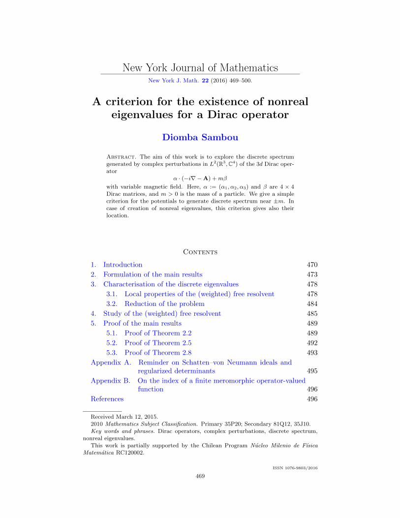
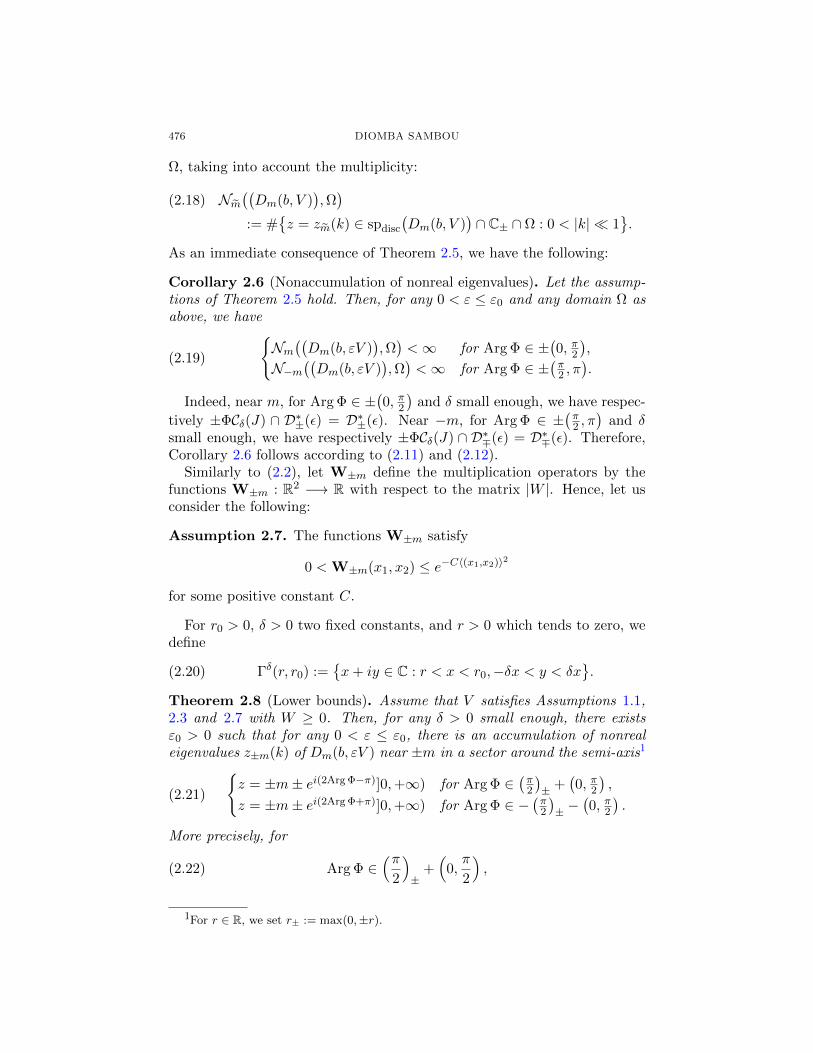
A graphic illustration of Theorems 2.5 and 2.8 near m with V = ΦW ,W ≥ 0, is given in Figure 2.

m η1 η2

eiArg ΦR+

π − Arg Φ

Re(z)

Im(z)y = tan(2Arg Φ− π) (x−m)

2θ

2θ

Sθ××××××××××

×××××

×××

××

V = ΦW

Arg Φ ∈ (π2 , π), W ≥ 0

Figure 2.1. Localisation of the nonreal eigenvalues near mwith 0 < η1 < η2 < η small enough: For θ small enough and0 < ε ≤ ε0, Dm(b, εV ) := Dm(b, 0)+εV has no eigenvalues inSθ (Theorem 2.5). They are concentrated around the semi-

axis z = m+ ei(2Arg Φ−π)]0,+∞) (Theorem 2.8).

Here, the accumulation of the nonreal eigenvalues of Dm(b, εV ) near ±mholds for any 0 < ε ≤ ε0. We expect this to be a general phenomenon inthe sense of the following conjecture:

Conjecture 2.9. Let V = ΦW satisfy Assumption 1.1 with

Arg Φ ∈ C \ Reikπ2 ,

k ∈ Z, and W Hermitian of definite sign. Then, for any domain Ω as in(2.18), we have

(2.25) N±m(Dm(b, V ),Ω

)<∞

if and only if ±Re(V ) > 0.

478 DIOMBA SAMBOU

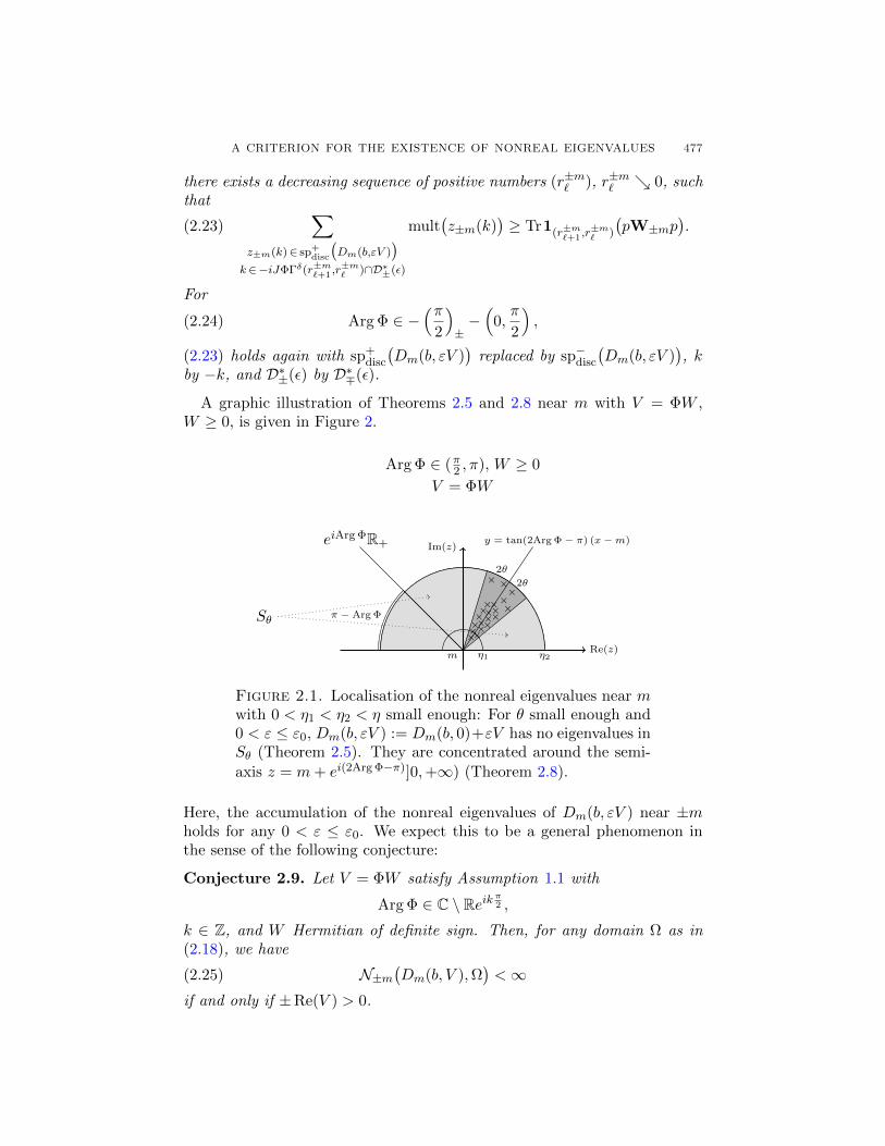
Figure 2.2. Summary of results.

3. Characterisation of the discrete eigenvalues

From now on, for m ∈ ±m, D±m(η) and D∗±(ε) are the domains givenby (2.6) and (2.7) respectively.

3.1. Local properties of the (weighted) free resolvent. In this sub-section, we show in particular that under Assumption 1.1, V is relativelycompact with respect to Dm(b, 0).

Let P := p ⊗ 1 define the orthogonal projection onto KerH−⊥ ⊗ L2(R),

where H−⊥ is the two-dimensional magnetic Schrdinger operator defined by(2.1). Denote P the orthogonal projection onto the union of the eigenspacesof Dm(b, 0) corresponding to ±m. Then, we have

(3.1) P =

(P 0 0 00 0 0 00 0 P 00 0 0 0

)and Q := I−P =

(I−P 0 0 0

0 I 0 00 0 I−P 00 0 0 I

),

(see [Sam13, Section 3]). Moreover, if z ∈ C \ (−∞,−m] ∪ [m,+∞), then

(3.2)(Dm(b, 0)− z

)−1=(Dm(b, 0)− z

)−1P +

(Dm(b, 0)− z

)−1Q

with

(Dm(b, 0)− z

)−1P =

[p⊗R(z2−m2)

]( z+m 0 0 00 0 0 00 0 z−m 00 0 0 0

)+[p⊗ (−i∂x3)R(z2 −m2)

]( 0 0 1 00 0 0 01 0 0 00 0 0 0

).

(3.3)

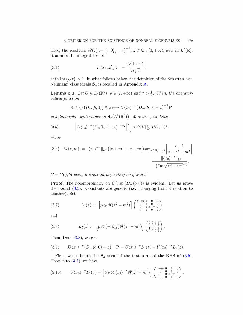
A CRITERION FOR THE EXISTENCE OF NONREAL EIGENVALUES 479

Here, the resolvent R(z) :=(−∂2

x3 − z)−1

, z ∈ C \ [0,+∞), acts in L2(R).It admits the integral kernel

(3.4) Iz(x3, x′3) := −e

i√z|x3−x′3|

2i√z

,

with Im(√z)> 0. In what follows below, the definition of the Schatten–von

Neumann class ideals Sq is recalled in Appendix A.

Lemma 3.1. Let U ∈ Lq(R2), q ∈ [2,+∞) and τ > 12 . Then, the operator-

valued function

C \ sp(Dm(b, 0)

)3 z 7−→ U〈x3〉−τ

(Dm(b, 0)− z

)−1P

is holomorphic with values in Sq(L2(R3)

). Moreover, we have

(3.5)

∥∥∥U〈x3〉−τ(Dm(b, 0)− z

)−1P

∥∥∥qSq≤ C‖U‖qLqM(z,m)q,

where

(3.6) M(z,m) := ‖〈x3〉−τ‖Lq(|z +m|+ |z −m|

)sups∈[0,+∞)

∣∣∣∣ s+ 1

s− z2 +m2

∣∣∣∣+

‖〈x3〉−τ‖L2(Im√z2 −m2

) 12

,

C = C(q, b) being a constant depending on q and b.

Proof. The holomorphicity on C \ sp(Dm(b, 0)

)is evident. Let us prove

the bound (3.5). Constants are generic (i.e., changing from a relation toanother). Set

(3.7) L1(z) :=[p⊗R(z2 −m2)

]( z+m 0 0 00 0 0 00 0 z−m 00 0 0 0

)and

(3.8) L2(z) :=[p⊗ (−i∂x3)R(z2 −m2)

]( 0 0 1 00 0 0 01 0 0 00 0 0 0

).

Then, from (3.3), we get

(3.9) U〈x3〉−τ(Dm(b, 0)− z

)−1P = U〈x3〉−τL1(z) + U〈x3〉−τL2(z).

First, we estimate the Sq-norm of the first term of the RHS of (3.9).Thanks to (3.7), we have

(3.10) U〈x3〉−τL1(z) =[Up⊗ 〈x3〉−τR(z2 −m2)

]( z+m 0 0 00 0 0 00 0 z−m 00 0 0 0

).

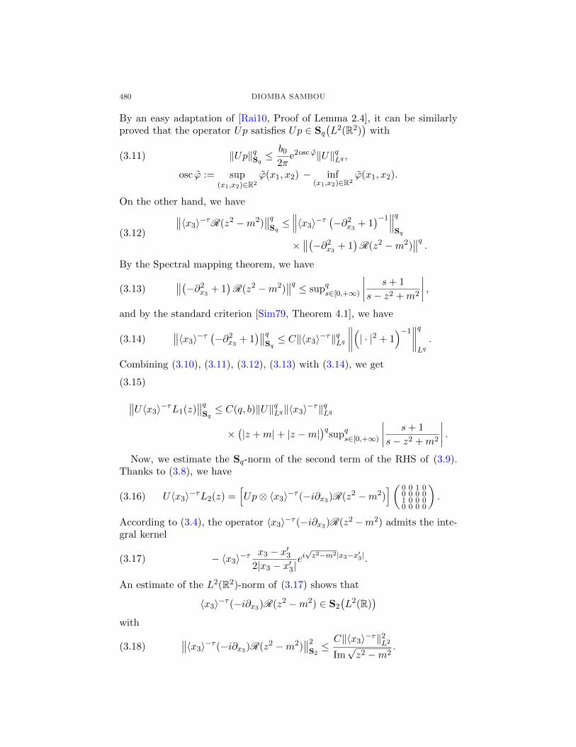
480 DIOMBA SAMBOU

By an easy adaptation of [Rai10, Proof of Lemma 2.4], it can be similarlyproved that the operator Up satisfies Up ∈ Sq

(L2(R2)

)with

‖Up‖qSq ≤b02π

e2osc ϕ‖U‖qLq ,(3.11)

osc ϕ := sup(x1,x2)∈R2

ϕ(x1, x2) − inf(x1,x2)∈R2

ϕ(x1, x2).

On the other hand, we have∥∥〈x3〉−τR(z2 −m2)∥∥qSq≤∥∥∥〈x3〉−τ

(−∂2

x3 + 1)−1∥∥∥qSq

×∥∥(−∂2

x3 + 1)R(z2 −m2)

∥∥q .(3.12)

By the Spectral mapping theorem, we have

(3.13)∥∥(−∂2

x3 + 1)R(z2 −m2)

∥∥q ≤ supqs∈[0,+∞)

∣∣∣∣ s+ 1

s− z2 +m2

∣∣∣∣ ,and by the standard criterion [Sim79, Theorem 4.1], we have

(3.14)∥∥〈x3〉−τ

(−∂2

x3 + 1)∥∥q

Sq≤ C‖〈x3〉−τ‖qLq

∥∥∥∥(| · |2 + 1)−1

∥∥∥∥qLq.

Combining (3.10), (3.11), (3.12), (3.13) with (3.14), we get

∥∥U〈x3〉−τL1(z)∥∥qSq≤ C(q, b)‖U‖qLq‖〈x3〉−τ‖qLq

(3.15)

×(|z +m|+ |z −m|

)qsupqs∈[0,+∞)

∣∣∣∣ s+ 1

s− z2 +m2

∣∣∣∣ .Now, we estimate the Sq-norm of the second term of the RHS of (3.9).

Thanks to (3.8), we have

(3.16) U〈x3〉−τL2(z) =[Up⊗ 〈x3〉−τ (−i∂x3)R(z2 −m2)

]( 0 0 1 00 0 0 01 0 0 00 0 0 0

).

According to (3.4), the operator 〈x3〉−τ (−i∂x3)R(z2 −m2) admits the inte-gral kernel

(3.17) − 〈x3〉−τx3 − x′3

2|x3 − x′3|ei√z2−m2|x3−x′3|.

An estimate of the L2(R2)-norm of (3.17) shows that

〈x3〉−τ (−i∂x3)R(z2 −m2) ∈ S2

(L2(R)

)with

(3.18)∥∥〈x3〉−τ (−i∂x3)R(z2 −m2)

∥∥2

S2≤C‖〈x3〉−τ‖2L2

Im√z2 −m2

.

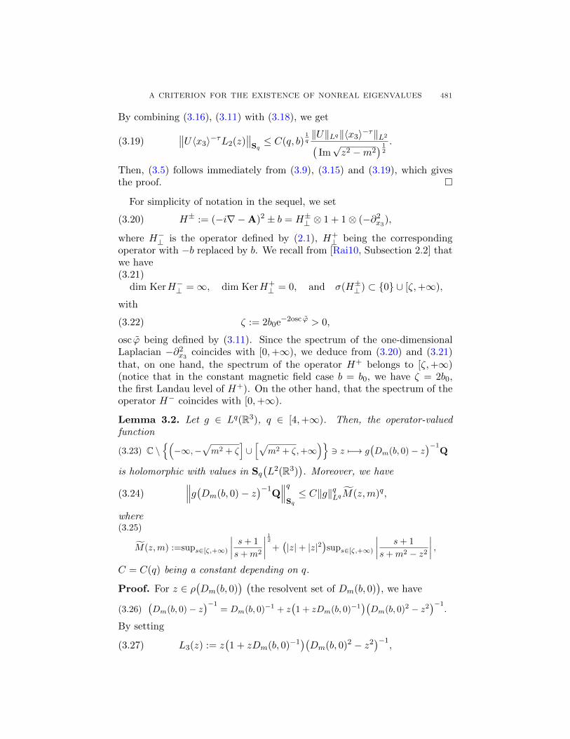
A CRITERION FOR THE EXISTENCE OF NONREAL EIGENVALUES 481

By combining (3.16), (3.11) with (3.18), we get

(3.19)∥∥U〈x3〉−τL2(z)

∥∥Sq≤ C(q, b)

1q‖U‖Lq‖〈x3〉−τ‖L2(

Im√z2 −m2

) 12

.

Then, (3.5) follows immediately from (3.9), (3.15) and (3.19), which givesthe proof.

For simplicity of notation in the sequel, we set

(3.20) H± := (−i∇−A)2 ± b = H±⊥ ⊗ 1 + 1⊗ (−∂2x3),

where H−⊥ is the operator defined by (2.1), H+⊥ being the corresponding

operator with −b replaced by b. We recall from [Rai10, Subsection 2.2] thatwe have(3.21)

dim KerH−⊥ =∞, dim KerH+⊥ = 0, and σ(H±⊥ ) ⊂ 0 ∪ [ζ,+∞),

with

(3.22) ζ := 2b0e−2osc ϕ > 0,

osc ϕ being defined by (3.11). Since the spectrum of the one-dimensionalLaplacian −∂2

x3 coincides with [0,+∞), we deduce from (3.20) and (3.21)that, on one hand, the spectrum of the operator H+ belongs to [ζ,+∞)(notice that in the constant magnetic field case b = b0, we have ζ = 2b0,the first Landau level of H+). On the other hand, that the spectrum of theoperator H− coincides with [0,+∞).

Lemma 3.2. Let g ∈ Lq(R3), q ∈ [4,+∞). Then, the operator-valuedfunction

(3.23) C \(−∞,−

√m2 + ζ

]∪[√

m2 + ζ,+∞)3 z 7−→ g

(Dm(b, 0)− z

)−1Q

is holomorphic with values in Sq(L2(R3)

). Moreover, we have

(3.24)∥∥∥g(Dm(b, 0)− z

)−1Q∥∥∥qSq≤ C‖g‖qLqM(z,m)q,

where(3.25)

M(z,m) :=sups∈[ζ,+∞)

∣∣∣∣ s+ 1

s+m2

∣∣∣∣ 12 +(|z|+ |z|2

)sups∈[ζ,+∞)

∣∣∣∣ s+ 1

s+m2 − z2

∣∣∣∣ ,C = C(q) being a constant depending on q.

Proof. For z ∈ ρ(Dm(b, 0)

) (the resolvent set of Dm(b, 0)

), we have

(3.26)(Dm(b, 0)− z

)−1= Dm(b, 0)−1 + z

(1 + zDm(b, 0)−1

)(Dm(b, 0)2 − z2

)−1.

By setting

(3.27) L3(z) := z(1 + zDm(b, 0)−1

)(Dm(b, 0)2 − z2

)−1,

482 DIOMBA SAMBOU

we get from (3.26)

(3.28) g(Dm(b, 0)− z

)−1Q = gDm(b, 0)−1Q + gL3(z)Q.

It can be proved that(Dm(b, 0)2 − z2

)−1Q(3.29)

=

(H−+m2−z2

)−1(I−P ) 0 0 0

0(H++m2−z2

)−10 0

0 0(H−+m2−z2

)−1(I−P ) 0

0 0 0(H++m2−z2

)−1

,(see for instance [TidA11, Identity (2.2)]). The set C \ [ζ,+∞) is includedin the resolvent set of H− defined on (I − P ) Dom(H−). Similarly, it isincluded in the resolvent set of H+ defined on Dom(H+). Then,(3.30)

C \(−∞,−

√m2 + ζ

]∪[√

m2 + ζ,+∞)3 z 7−→

(Dm(b, 0)2 − z2

)−1Q

is well defined and holomorphic. Therefore, so is the operator-valued func-tion (3.23) thanks to (3.27) and (3.28).

It remains to prove the bound (3.24). As in the proof of the previouslemma, the constants change from a relation to another. First, we provethat (3.24) is true for q even.

Let us focus on the second term of the RHS of (3.28). According to (3.27)and (3.29), we have

‖gL3(z)Q‖qSq

(3.31)

≤ C(|z|+ |z|2

)q×(∥∥∥g(H− +m2 − z2

)−1(I − P )

∥∥∥qSq

+∥∥∥g(H+ +m2 − z2

)−1∥∥∥qSq

).

One has ∥∥∥g(H− +m2 − z2)−1

(I − P )∥∥∥qSq

(3.32)

≤∥∥g(H− + 1)−1

∥∥qSq

∥∥∥(H− + 1)(H− +m2 − z2

)−1(I − P )

∥∥∥q .The Spectral mapping theorem implies that

(3.33)∥∥∥(H− + 1)

(H− +m2 − z2

)−1(I − P )

∥∥∥q ≤ supqs∈[ζ,+∞)

∣∣∣∣ s+ 1

s+m2 − z2

∣∣∣∣ .Exploiting the resolvent equation, the boundedness of b, and the diamagneticinequality (see [AHS78, Theorem 2.3] and [Sim79, Theorem 2.13], which is

A CRITERION FOR THE EXISTENCE OF NONREAL EIGENVALUES 483

only valid when q is even), we obtain

∥∥∥g(H− + 1)−1∥∥∥qSq≤∥∥I + (H− + 1)−1b

∥∥q ∥∥∥g((−i∇−A)2 + 1)−1∥∥∥qSq

≤ C∥∥g(−∆ + 1)−1

∥∥qSq.

(3.34)

The standard criterion [Sim79, Theorem 4.1] implies that

(3.35)∥∥g(−∆ + 1|)−1

∥∥qSq≤ C‖g‖qLq

∥∥∥∥(| · |2 + 1)−1

∥∥∥∥qLq.

The bound (3.32) together with (3.33), (3.34) and (3.35) give

(3.36)∥∥∥g(H− +m2 − z2

)−1(I − P )

∥∥∥qSq≤ C‖g‖qLqsupqs∈[ζ,+∞)

∣∣∣∣ s+ 1

s+m2 − z2

∣∣∣∣ .Similarly, it can be shown that

(3.37)∥∥∥g(H+ +m2 − z2

)−1∥∥∥qSq≤ C‖g‖qLqsupqs∈[ζ,+∞)

∣∣∣∣ s+ 1

s+m2 − z2

∣∣∣∣ .This together with (3.31) and (3.36) give

(3.38) ‖gL3(z)Q‖qSq ≤ C‖g‖qLq

(|z|+ |z|2

)qsupqs∈[ζ,+∞)

∣∣∣∣ s+ 1

s+m2 − z2

∣∣∣∣ .Now, we focus on the first term gDm(b, 0)−1Q of the RHS of (3.28). For

γ > 0, as in (3.29), we have

Dm(b, 0)−γQ(3.39)

=

(H−+m2

)− γ2 (I−P ) 0 0 0

0(H++m2

)− γ2 0 0

0 0(H−+m2

)− γ2 (I−P ) 0

0 0 0(H++m2

)− γ2

.

Therefore, arguing as above((3.31)–(3.37)

), it can be proved that

(3.40)∥∥gDm(b, 0)−γQ∥∥qSq≤ C(q, γ)‖g‖qLqsupqs∈[ζ,+∞)

∣∣∣∣ s+ 1

s+m2

∣∣∣∣ γ2 , γq > 3.

Then, for q even, (3.24) follows by putting together (3.28), (3.38), and (3.40)with γ = 1.

We get the general case q ≥ 4 with the help of interpolation methods.If q satisfies q > 4, then, there exists even integers q0 < q1 such that

q ∈ (q0, q1) with q0 ≥ 4. Let β ∈ (0, 1) satisfy 1q = 1−β

q0+ β

q1and consider

the operator

Lqi(R3)3 g T7−→ g

(Dm(b, 0)− z

)−1Q ∈ Sqi

(L2(R3)

), i = 0, 1.

Let Ci = C(qi), i = 0, 1, denote the constant appearing in (3.24) and set

C(z, qi) := C1qii M(z,m).

484 DIOMBA SAMBOU

From (3.24), we know that ‖T‖ ≤ C(z, qi), i = 0, 1. Now, we use the Riesz–Thorin Theorem (see for instance [Fol84, Sub. 5 of Chap. 6], [Rie26, Tho39],[Lun09, Chap. 2]) to interpolate between q0 and q1. We obtain the extensionT : Lq(R2) −→ Sq

(L2(R3)

)with

‖T‖ ≤ C(z, q0)1−βC(γ, q1)β ≤ C(q)1q M(z,m).

In particular, for any g ∈ Lq(R3), we have

‖T (g)‖Sq ≤ C(q)1q M(z,m)‖g‖Lq ,

which is equivalent to (3.24). This completes the proof.

Assumption 1.1 ensures the existence of V ∈ L(L2(R3)

)such that for

any x ∈ R3,

(3.41) |V |12 (x) = V F

12⊥ (x1, x2)G

12 (x3).

Therefore, the boundedness of V together with Lemmas 3.1–3.2, (3.2), and(3.41), imply that V is relatively compact with respect to Dm(b, 0).

Since for k ∈ D∗±(ε) we have

zm(k) =m(1 + k2)

1− k2∈ C \

(−∞,−m] ∪ [m,+∞)

,

where m ∈ ±m, then this together with Lemmas 3.1–3.2, (3.2) and (3.41)give the following:

Lemma 3.3. For m ∈ ±m and zm(k) = m(1+k2)1−k2 , the operator-valued

functions

D∗±(ε) 3 k 7−→ TV(zm(k)

):= J |V |

12(Dm(b, 0)− zm(k)

)−1|V |12

are holomorphic with values in Sq(L2(R3)

), J being defined by the polar

decomposition V = J |V |.

3.2. Reduction of the problem. We show how we can reduce the inves-tigation of the discrete spectrum of Dm(b, V ) to that of zeros of holomorphicfunctions.

In the sequel, the definition of the q-regularized determinant detdqe(·) isrecalled in Appendix A by (A.2). As in Lemma 3.3, the operator-valued

function V(Dm(b, 0)−·

)−1is analytic on D±m(η) with values in Sq

(L2(R3)

).

Hence, the following characterisation(3.42)

z ∈ spdisc

(Dm(b, V )

)⇔ f(z) := detdqe

(I + V

(Dm(b, 0)− z

)−1)

= 0

holds; see for instance [Sim79, Chap. 9] for more details. The fact that theoperator-valued function V

(Dm(b, 0) − ·

)is holomorphic on D±m(η) implies

that the same happens for the function f(·) by Property (d) of Appen-dix A. Furthermore, the algebraic multiplicity of z as discrete eigenvalue of

A CRITERION FOR THE EXISTENCE OF NONREAL EIGENVALUES 485

Dm(b, V ) is equal to its order as zero of f(·) (this claim is a well known fact,see for instance [Han15, Proof of Theorem 4.10 (v)] for an idea of proof).

In the next proposition, the quantity IndC (·) in the RHS of (3.43) isrecalled in Appendix B by (B.2).

Proposition 3.4. The following assertions are equivalent:

(i) zm(k0) =m(1+k20)

1−k20∈ D±m(η) is a discrete eigenvalue of Dm(b, V ).

(ii) detdqe(I + TV

(zm(k0)

) )= 0.

(iii) −1 is an eigenvalue of TV(zm(k0)

).

Moreover,

(3.43) mult(zm(k0)

)= IndC

(I + TV

(zm(·)

)),

C being a small contour positively oriented, containing k0 as the unique pointk ∈ D∗±(ε) verifying zm(k) ∈ D±m(η) is a discrete eigenvalue of Dm(b, V ).

Proof. The equivalence (i)⇔(ii) follows obviously from (3.42) and the equal-ity

detdqe

(I + V

(Dm(b, 0)− z

)−1)

= detdqe

(I + J |V |

12(Dm(b, 0)− z

)−1|V |12

),

see Property (b) of Appendix A.The equivalence (ii)⇔(iii) is a direct consequence of Property (c) of Ap-

pendix A.It only remains to prove (3.43). According to the discussion just after

(3.42), for C ′ a small contour positively oriented containing zm(k0) as theunique discrete eigenvalue of Dm(b, V ), we have

(3.44) mult(zm(k0)

)= IndC ′ f,

f being the function defined by (3.42). The RHS of (3.44) is the indexdefined by (B.1), of the holomorphic function f with respect to C ′. Now,(3.43) follows directly from the equality

IndC ′ f = IndC

(I + TV

(zm(·)

)),

see for instance [BBR14, (2.6)] for more details.

4. Study of the (weighted) free resolvent

We split TV(zm(k)

)into a singular part at k = 0, and an analytic part in

D∗±(ε) which is continuous on D∗±(ε), with values in Sq(L2(R3)

).

486 DIOMBA SAMBOU

For z := z±m(k), set

T V1(z±m(k)

):= J |V |1/2

[p⊗R

(k2(z ±m)2

)]( z+m 0 0 00 0 0 00 0 z−m 00 0 0 0

)|V |1/2,

(4.1)

T V2(z±m(k)

):= J |V |1/2

[p⊗ (−i∂x3)R

(k2(z ±m)2

)]( 0 0 1 00 0 0 01 0 0 00 0 0 0

)|V |1/2

(4.2)

+ J |V |1/2(Dm(b, 0)− z

)−1Q|V |1/2.

Then, (3.2) combined with (3.3) imply that

(4.3) TV(z±m(k)

)= T V1

(z±m(k)

)+ T V2

(z±m(k)

).

Remark 4.1.

(i) For z = zm(k), we have

(4.4) Im(k(z +m)

)=

2m(1 + |k|2) Im(k)

|1 + k2|2.

Therefore, according to the choice (2.5) of the complex square root,we have respectively

(4.5)√k2(z +m)2 = ±k(z +m) for k ∈ D∗±(ε).

(ii) In the case z = z−m(k), we have

(4.6) Im(k(z −m)

)= −2m(1 + |k|2) Im(k)

|1 + k2|2,

so that

(4.7)√k2(z −m)2 = ∓k(z −m) for k ∈ D∗±(ε).

In what follows below, we focus on the study of the operator TV(zm(k)

),

i.e., near m. The same arguments yield that of the operator TV(z−m(k)

)associated to −m (see Remark 4.3).

Defining G± as the multiplication operators by the functions

G± : R 3 x3 7→ G±12 (x3),

we have

(4.8) T V1(zm(k)

)=

J |V |1/2G−[p⊗G+R

(k2(z +m)2

)G+

]( z+m 0 0 00 0 0 00 0 z−m 00 0 0 0

)G−|V |1/2.

Remark 4.1(i) together with (3.4) imply that G+R(k2(z +m)2

)G+ admits

the integral kernel

(4.9) ±G12 (x3)

ie±ik(z+m)|x3−x′3|

2k(z +m)G

12 (x′3), k ∈ D∗±(ε).

A CRITERION FOR THE EXISTENCE OF NONREAL EIGENVALUES 487

Then, from (4.9) we deduce that

(4.10) G+R(k2(z +m)2

)G+ = ± 1

k(z +m)a+ bm(k), k ∈ D∗±(ε),

where a : L2(R) −→ L2(R) is the rank-one operator given by

(4.11) a(u) :=i

2

⟨u,G+

⟩G+,

and bm(k) is the operator with integral kernel

(4.12) ±G12 (x3)i

e±ik(z+m)|x3−x′3| − 1

2k(z +m)G

12 (x′3).

Note that −2ia = c∗c, where c : L2(R) −→ C satisfies c(u) := 〈u,G+〉 andc∗ : C −→ L2(R) verifies c∗(λ) = λG+. Therefore, by combining (4.10),(4.11) with (4.12), we get for k ∈ D∗±(ε)

(4.13) p⊗G+R(k2(z +m)2

)G+ = ± i

2k(z +m)p⊗ c∗c+ p⊗ sm(k),

where sm(k) is the operator acting from G12 (x3)L2(R) to G−

12 (x3)L2(R)

with integral kernel

(4.14) ± 1− e±ik(z+m)|x3−x′3|

2ik(z +m).

In Remark 4.3, s−m(k) is the corresponding operator with m replaced by−m and ± replaced by ∓ in (4.14). Now, putting together (4.8) and (4.13),we get for k ∈ D∗±(ε)

T V1(zm(k)

)= ± iJ

2k(z +m)|V |

12G−(p⊗ c∗c)

(z+m 0 0 0

0 0 0 00 0 z−m 00 0 0 0

)G−|V |

12

(4.15)

+ J |V |12G−p⊗ sm(k)

(z+m 0 0 0

0 0 0 00 0 z−m 00 0 0 0

)G−|V |

12 .

Introduce the operator

(4.16) K±m :=1√2

(p⊗ c)

(1−1∓ 0 0 0

0 0 0 00 0 1−1± 00 0 0 0

)G−|V |

12 , 1− = 0, 1+ = 1.

It is well known from [Hal98, Theorem 2.3] that p admits a continuousintegral kernel P(x⊥, x

′⊥), x⊥, x′⊥ ∈ R2. Then, we have

K±m : L2(R3) −→ L2(R2)

488 DIOMBA SAMBOU

with

(K±mψ)(x⊥)

=1√2

∫R3

P(x⊥, x′⊥)

(1−1∓ 0 0 0

0 0 0 00 0 1−1± 00 0 0 0

)|V |

12 (x′⊥, x

′3)ψ(x′⊥, x

′3)dx′⊥dx

′3.

Obviously, the operator K∗±m : L2(R2) −→ L2(R3) satisfies

(K∗±mϕ)(x⊥, x3) =1√2|V |

12 (x⊥, x3)

(1−1∓ 0 0 0

0 0 0 00 0 1−1± 00 0 0 0

)(pϕ)(x⊥).

Noting that K±mK∗±m : L2(R2) −→ L2(R2) verifies

(4.17) K±mK∗±m =

(1−1∓ 0 0 0

0 0 0 00 0 1−1± 00 0 0 0

)pV±mp,

V±m being the multiplication operators by the functions (also noted) V±mdefined by (2.2). Thus, by combining (4.15) and (4.16) we obtain for k ∈D∗±(ε)

T V1(zm(k)

)= ± iJ

kK∗mKm + iJkK∗−mK−m(4.18)

+ J |V |12G−p⊗ sm(k)

(z+m 0 0 0

0 0 0 00 0 z−m 00 0 0 0

)G−|V |

12 .

Now, for λ ∈ R∗+, we define(− ∂2

x3 − λ)−1

as the operator with integralkernel

(4.19) Iλ(x3, x′3) := lim

δ↓0Iλ+iδ(x3, x

′3) =

iei√λ|x3−x′3|

2√λ

.

Here Iz(·) is given by (3.4). Therefore, it can be proved, using a limitingabsorption principle, that the operator-valued functions

D∗±(ε) 3 k 7→ G+sm(k)G+ ∈ S2

(L2(R)

)are well defined and continuous similarly to [Rai10, Proposition 4.2]. Wethus arrive to the following:

Proposition 4.2. Let k ∈ D∗±(ε). Then,

(4.20) TV(zm(k)

)= ± iJ

kBm + Am(k), Bm := K∗mKm,

where Am(k) ∈ Sq(L2(R3)

)given by

Am(k) := iJkK∗−mK−m+J |V |12G−p⊗ sm(k)

×(z+m 0 0 0

0 0 0 00 0 z−m 00 0 0 0

)G−|V |

12 + T V2

(zm(k)

)is holomorphic in D∗±(ε) and continuous on D∗±(ε).

A CRITERION FOR THE EXISTENCE OF NONREAL EIGENVALUES 489

Remark 4.3.

(i) Identity (4.17) implies that for any r > 0, we have

(4.21) Tr1(r,∞)

(K∗±mK±m

)= Tr1(r,∞)

(K±mK

∗±m)

= Tr1(r,∞)

(pV±mp

).

(ii) For V verifying Assumption 2.3, Proposition 4.2 holds with J re-placed by JΦ, J := sign(W ), and in (4.21) V±m replaced by W±m.

(iii) Near −m, taking into account Remark 4.1(ii), Proposition 4.2 holdswith

(4.22) TV(z−m(k)

)= ∓ iJ

kB−m + A−m(k), B−m := K∗−mK−m,

and

A−m(k) := iJkK∗mKm+J |V |12G−p⊗ s−m(k)

×(z+m 0 0 0

0 0 0 00 0 z−m 00 0 0 0

)G−|V |

12 + T V2

(z−m(k)

).

5. Proof of the main results

5.1. Proof of Theorem 2.2. It suffices to prove that both sums in theLHS of (2.14) are bounded by the RHS. We only give the proof for the firstsum. For the second one, the estimate follows similarly by using Remark2.1(iii),(iv), Proposition 4.2, and Remark 4.3(i),(iii).

In what follows below,

N(Dm(b, V )

):=〈Dm(b, V )f, f〉 : f ∈ Dom

(Dm(b, V )

), ‖f‖L2 = 1

denotes the numerical range of the operator Dm(b, V ). It satisfies the inclu-

sion sp(Dm(b, V )

)⊆ N

(Dm(b, V )

), see, e.g., [Dav07, Lemma 9.3.14].

The proof of the theorem uses the following:

Proposition 5.1. Let 0 < s0 < ε be small enough. Then, for any

k ∈ 0 < s < |k| < s0 ∩ D∗±(ε),

the following properties hold:

(i) z±m(k) ∈ sp+disc

(Dm(b, V )

)near ±m if and only if k is a zero of the

determinants

(5.1) D±m(k, s) := det(I + K±m(k, s)

),

where K±m(k, s) are finite-rank operators analytic with respect to ksuch that

(5.2) rank K±m(k, s) = O(

Tr1(s,∞)

(pV±mp

)+ 1), ‖K±m(k, s)‖ = O

(s−1),

uniformly with respect to s < |k| < s0.

490 DIOMBA SAMBOU

(ii) Moreover, if z±m(k0) ∈ sp+disc

(Dm(b, V )

)near ±m, then

(5.3) mult(z±m(k0)

)= IndC

(I + K±m(·, s)

)= mult(k0),

where C is chosen as in (3.43), and mult(k0) is the multiplicity ofk0 as zero of D±m(·, s).

(iii) If z±m(k) satisfies

dist(z±m(k), N

(Dm(b, V )

))> ς > 0,

then I + K±m(k, s) are invertible and satisfy∥∥∥(I + K±m(k, s))−1∥∥∥ = O

(ς−1)

uniformly with respect to s < |k| < s0.

Proof. (i)–(ii) By Proposition 4.2 and Remark 4.3(iii), the operator-valuedfunctions

(5.4) k 7→ A±m(k) ∈ Sq(L2(R3)

)are continuous near zero. Then, for s0 small enough, there exists A0,±m

finite-rank operators which do not depend on k, and A±m(k) ∈ Sq(L2(R3)

)continuous near zero satisfying ‖A±m(k)‖ < 1

4 for |k| ≤ s0, such that

(5.5) A±m(k) = A0,±m + A±m(k).

Let B±m be the operators defined respectively by (4.20) and (4.22). Then,with the help of the decomposition

(5.6) B±m = B±m1[0, 12s](B±m) + B±m1] 1

2s,∞[(B±m),

and using that∥∥∥± iJ

k B±m1[0, 12s](B±m) + A±m(k)

∥∥∥ < 34 for 0 < s < |k| < s0,

we obtain

(5.7)(I + TV

(z±m(k)

))=(I + K±m(k, s)

)(I ± iJ

kB±m1[0, 1

2s](B±m) + A±m(k)

),

where

K±m(k, s) :=

(± iJk

B±m1] 12s,∞[(B±m) + A0,±m

)(5.8)

×

(I ± iJ

kB±m1[0, 1

2s](B±m) + A±m(k)

)−1

.

Observe that K±m(k, s) are finite-rank operators with ranks of order

(5.9) O(

Tr1( 12 s,∞)(B±m) + 1

)= O

(Tr1(s,∞)

(pV±mp

)+ 1),

A CRITERION FOR THE EXISTENCE OF NONREAL EIGENVALUES 491

according to (4.21). Moreover, their norms are of order O(|k|−1

)= O

(s−1).

From above we know that for 0 < s < |k| < s0 we have∥∥∥∥∥± iJk B±m1[0, 12s](B±m) + A±m(k)

∥∥∥∥∥ < 3

4< 1.

Then, we obtain

(5.10) IndC

(I ± iJ

kB±m1[0, 12 s]

(B±m) + A (k)

)= 0

from [GohGK90, Theorem 4.4.3]. Therefore, equalities (5.3) follow by ap-plying to (5.7) the properties of the index of a finite meromorphic operator-valued function recalled in the Appendix B. Proposition 3.4 together with(5.7) imply that z±m(k) belongs to sp+

disc

(Dm(b, V )

)near ±m if and only if

k is a zero of the determinants D±m(k, s) defined by (5.1).

(iii) From (5.7), we deduce that

(5.11) I + K±m(k, s)

=(I + TV

(z±m(k)

))(I +

J

kB±m1[0, 1

2s](B±m) + A±m(k)

)−1

,

for 0 < s < |k| < s0. With the help of the resolvent equation, it can beshown that

(5.12) I =(I+ J |V |1/2

(Dm(b, 0)−z

)−1|V |1/2)(I− J |V |1/2

(Dm(b, V )−z

)−1|V |1/2).

Then, for z±m(k) ∈ ρ(Dm(b, V )

), obviously we have

(5.13)(I + TV

(z±m(k)

))−1= I − J |V |1/2

(Dm(b, V )− z±m(k)

)−1|V |1/2.

This together with (5.11) imply the invertibility of I + K±m(k, s) for 0 <s < |k| < s0, and according to [Dav07, Lemma 9.3.14] it satisfies∥∥∥(I + K±m(k, s)

)−1∥∥∥ = O

(1 +

∥∥∥|V |1/2(Dm(b, V )− z±m(k))−1|W |1/2

∥∥∥)= O

(1 + dist

(z±m(k), N

(Dm(b, V )

))−1)

= O(ς−1),

for dist(z±m(k), N

(Dm(b, V )

))> ς > 0. This completes the proof.

492 DIOMBA SAMBOU

End of the proof of Theorem 2.2. Now, from Proposition 5.1(i), we ob-tain for 0 < s < |k| < s0

D±m(k, s) =

O(

Tr1(s,∞)(pV±mp)+1)∏

j=1

(1 + λj,±m(k, s)

)(5.14)

= O(1) exp(O(Tr1(s,∞)

(pV±mp

)+ 1)| ln s|

),

where the λj,±m(k, s) are the eigenvalues of K±m := K±m(k, s) which satisfy|λj,±m(k, s)| = O

(s−1)

so that ln∣∣1 + λj,±m(k, s)

∣∣ = O(| ln s|

)(for s small

enough). Otherwise, we have for 0 < s < |k| < s0

D±m(k, s)−1 = det(I + K±m

)−1= det

(I −K±m(I + K±m)−1

)if dist

(z±m(k), N

(Dm(b, V )

))> ς > 0. Then, as in (5.14), it can be shown

that

(5.15) |D±m(k, s)| ≥ C exp(− C

(Tr1(s,∞)

(pV±mp

)+ 1)(|ln ς|+ |ln s|

)).

To conclude, we need the following Jensen lemma (see for instance [BBR07,Lemma 6] for a simple proof).

Lemma 5.2. Let ∆ be a simply connected sub-domain of C and let g beholomorphic in ∆ with continuous extension to ∆. Assume that there existsλ0 ∈ ∆ such that g(λ0) 6= 0 and g(λ) 6= 0 for λ ∈ ∂∆ (the boundaryof ∆). Let λ1, λ2, . . . , λN ∈ ∆ be the zeros of g repeated according to theirmultiplicity. For any domain ∆′ b ∆, there exists C ′ > 0 such that N(∆′, g),the number of zeros λj of g contained in ∆′ satisfies

(5.16) N(∆′, g) ≤ C ′(∫

∂∆ln|g(λ)|dλ− ln|g(λ0)|

).

Consider the domains

∆± :=r < |k| < 2r : |Re(k)| >

√ν : |Im(k)| >

√ν : ν > 0

∩ D∗±(ε)

with 0 < r < ε/2, and some k0 ∈ ∆± satisfying

dist(z±m(k0), N

(Dm(b, V )

))> ς > 0.

Then, we get that the first sum in the LHS of (2.14) is bounded by the RHSby using Lemma 5.2 with the functions g = g±m(k) := D±m(k, r), togetherwith (5.14) and (5.15). This concludes the proof of Theorem 2.2.

5.2. Proof of Theorem 2.5. It will only be given for the case Arg Φ ∈(0, π). To prove the case Arg Φ ∈ −(0, π), it suffices to argue similarly byreplacing k by −k.

Remark 2.4(i), together with Proposition 4.2 and Remark 4.3(ii),(iii),imply that

(5.17) TεV(z±m(k)

)=iJεΦ

kB±m + εA±m(k), k ∈ D∗±(ε),

A CRITERION FOR THE EXISTENCE OF NONREAL EIGENVALUES 493

where B±m are positive self-adjoint operators which do not depend on k,and A±m(k) ∈ Sq

(L2(R3)

)are holomorphic in D∗±(ε) and continuous on

D∗±(ε). Noting that

(5.18) I +iJεΦ

kB±m =

iJΦ

k(εB±m − iJkΦ−1),

it is easy to see that I + iJεΦk B±m are invertible whenever iJkΦ−1 /∈

sp (εB±m). Moreover, we have

(5.19)

∥∥∥∥∥(I +

iJεΦ

kB±m

)−1∥∥∥∥∥ ≤ |k|√(

J Im(kΦ−1))2

++ |Re(kΦ−1)|2

.

Therefore,

(5.20)

∥∥∥∥∥(I +

iJεΦ

kB±m

)−1∥∥∥∥∥ ≤√1 + δ−2

for k ∈ ΦCδ(J), uniformly with respect to 0 < |k| < r0. Then, we deducefrom (5.17) that

(5.21) I + TεV(z±m(k)

)=(I +A±m(k)

)(I +

iJεΦ

kB±m

),

where

(5.22) A±m(k) := εA±m(k)

(I +

iJεΦ

kB±m

)−1

∈ Sq(L2(R3)

).

Now, by exploiting the continuity of A±m(k) ∈ Sq(L2(R3)

)near k = 0, it

can be proved that ‖A±m(k)‖ ≤ C for some C > 0 constant (not dependingon k). This together with (5.20) and (5.22) imply clearly the invertibility of

I + TεV(z±m(k)

)for k ∈ ΦCδ(J) and ε <

(C√

1 + δ−2)−1

. Thus, z±m(k) isnot a discrete eigenvalue near ±m.

5.3. Proof of Theorem 2.8. Denote (µ±mj )j the sequences of the decreas-ing nonzero eigenvalues of pW±mp taking into account the multiplicity. IfAssumption 2.3 holds, it can be proved that there exists a constant ν±m > 0such that

(5.23) #j : µ±mj − µ±mj+1 > ν±mµ

±mj

=∞.

Since B±m and pW±mp have the same nonzero eigenvalues, then, thereexist decreasing sequences (r±m` )`, r

±m` 0 with r±m` > 0, such that

(5.24) dist(r±m` , sp (B±m)

)≥νr±m`

2, ` ∈ N.

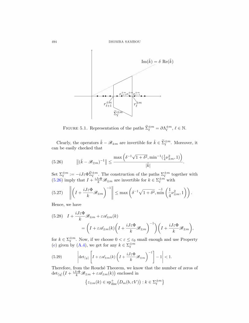
Furthermore, there exists paths Σ±m` := ∂Λ±m` with

(5.25) Λ±m` :=k ∈ C : 0 < |k| < r0 : | Im(k)| ≤ δRe(k) : r±m`+1 ≤ Re(k) ≤ r±m`

,

(see Figure 5.1) enclosing the eigenvalues of B±m lying in [r±m`+1, r±m` ].

494 DIOMBA SAMBOU

Im(k) = δ Re(k)

Σ±m`

r±m`+1 r±m`

•µ±mj •

µ±mj−1• • •

µ±mj+1••• • •

Figure 5.1. Representation of the paths Σ±m` = ∂Λ±m` , ` ∈ N.

Clearly, the operators k −B±m are invertible for k ∈ Σ±m` . Moreover, itcan be easily checked that

(5.26)∥∥(k −B±m)−1

∥∥ ≤ max(δ−1√

1 + δ2,min−1(14ν

2±m, 1)

)|k|

.

Set Σ±m` := −iJεΦΣ±m` . The construction of the paths Σ±m` together with

(5.26) imply that I + iJεΦk B±m are invertible for k ∈ Σ±m` with

(5.27)

∥∥∥∥∥(I +

iJεΦ

kB±m

)−1∥∥∥∥∥ ≤ max

(δ−1√

1 + δ2,−1

min

(1

4ν2±m, 1

)).

Hence, we have

(5.28) I +iJεΦ

kB±m + εA±m(k)

=

(I + εA±m(k)

(I +

iJεΦ

kB±m

)−1)(I +

iJεΦ

kB±m

),

for k ∈ Σ±m` . Now, if we choose 0 < ε ≤ ε0 small enough and use Property

(e) given by (A.4), we get for any k ∈ Σ±m`

(5.29)

∣∣∣∣∣detdqe

[I + εA±m(k)

(I +

iJεΦ

kB±m

)−1]− 1

∣∣∣∣∣ < 1.

Therefore, from the Rouche Theorem, we know that the number of zeros ofdetdqe

(I + iJεΦ

k B±m + εA±m(k))

enclosed inz±m(k) ∈ sp+

disc

(Dm(b, εV )

): k ∈ Σ±m`

A CRITERION FOR THE EXISTENCE OF NONREAL EIGENVALUES 495

taking into account the multiplicity, coincides with that of

detdqe

(I +

iJεΦ

kB±m

)enclosed in

z±m(k) ∈ sp+

disc

(Dm(b, εV )

): k ∈ Σ±m`

taking into account

the multiplicity. The number of zeros of detdqe(I + iJεΦ

k B±m)

enclosed inz±m(k) ∈ sp+

disc

(Dm(b, εV )

): k ∈ Σ±m`

taking into account the multiplic-

ity is equal to Tr1[r±m`+1,r±m` ]

(pW±mp

). The zeros of

detdqe

(I +

iJεΦ

kB±m + εA±m(k)

)are the discrete eigenvalues of Dm(b, εV ) near ±m taking into account themultiplicity. Then, this together with Proposition 3.4 and Property (B.3)applied to (5.28) give estimate (2.23). Since the sequences (r±m` )` are in-finite tending to zero, then the infiniteness of the number of the discreteeigenvalues claimed follows, which completes the proof of Theorem 2.8.

Appendix A. Reminder on Schatten–von Neumann idealsand regularized determinants

Consider a separable Hilbert space H . Let S∞(H ) denote the set ofcompact linear operators on H , and sk(T ) be the k-th singular value ofT ∈ S∞(H ). For q ∈ [1,+∞), the Schatten–von Neumann classes aredefined by

(A.1) Sq(H ) :=T ∈ S∞(H ) : ‖T‖qSq :=

∑k

sk(T )q < +∞.

When no confusion can arise, we write Sq for simplicity. If T ∈ Sq withdqe := min

n ∈ N : n ≥ q

, the q-regularized determinant is defined by

(A.2) detdqe(I − T ) :=∏

µ ∈ σ(T )

(1− µ) exp

dqe−1∑k=1

µk

k

.In particular, when q = 1, to simplify the notation we set

(A.3) det(I − T ) := detd1e(I − T ).

Let us give (see for instance [Sim77]) some elementary useful properties onthis determinant.

(a) We have detdqe(I) = 1.(b) If A, B ∈ L (H ) with AB and BA lying in Sq, then detdqe(I −

AB) = detdqe(I − BA). Here, L (H ) is the set of bounded linearoperators on H .

(c) I − T is an invertible operator if and only if detdqe(I − T ) 6= 0.(d) If T : Ω −→ Sq is a holomorphic operator-valued function on a

domain Ω, then so is detdqe(I − T (·)

)on Ω.

496 DIOMBA SAMBOU

(e) As function on Sq, detdqe(I − T ) is Lipschitz uniformly on balls.This means that

(A.4)∣∣detdqe(I − T1)− detdqe(I − T2)

∣∣≤ ‖T1 − T2‖Sq exp

(Γq(‖T1‖Sq + ‖T2‖Sq + 1

)dqe),

[Sim77, Theorem 6.5].

Appendix B. On the index of a finite meromorphicoperator-valued function

We refer for instance to [GohL09] for the definition of a finite meromorphicoperator-valued function.

Let f : Ω → C be a holomorphic function in a vicinity of a contour Cpositively oriented. Then, it index with respect to C is given by

(B.1) IndC f :=1

2iπ

∫C

f ′(z)

f(z)dz.

Observe that if ∂Ω = C , then indC f is equal to the number of zeros of flying in Ω taking into account their multiplicity (by the residues theorem).

If D ⊆ C is a connected domain, Z ⊂ D a closed pure point subset,A : D\Z −→ GL(H ) a finite meromorphic operator-valued function whichis Fredholm at each point of Z, the index of A with respect to the contour∂Ω is given by

(B.2) Ind∂Ω A :=1

2iπTr

∫∂Ω

A′(z)A(z)−1dz =1

2iπTr

∫∂Ω

A(z)−1A′(z)dz.

We have the following well known properties:

(B.3) Ind∂Ω A1A2 = Ind∂Ω A1 + Ind∂Ω A2;

if K(z) is of trace-class, then

(B.4) Ind∂Ω (I +K) = Ind∂Ω det (I +K),

see for instance to [GohGK90, Chap. 4] for more details.

References

[AHS78] Avron, J.; Herbst, I.; Simon, B. Schrodinger operators with magnetic fields.I. General interactions. Duke Math. J. 45 (1978), no. 4, 847–883. MR0518109,Zbl 0399.35029, doi: 10.1215/S0012-7094-78-04540-4.

[Beh13] Behrndt, Jussi. An open problem: accumulation of nonreal eigenvalues ofindefinite Sturm–Liouville operators. Integral Equations Operator Theory 77(2013), no. 3, 299–301. MR3116661, Zbl 1283.47052, doi: 10.1007/s00020-013-2065-1.

[BBR07] Bony, Jean-Francois; Bruneau, Vincent; Raikov, Georgi. Resonancesand spectral shift function near the Landau levels. Ann. Inst. Fourier (Grenoble)57 (2007), no. 2, 629–671. MR2310953, Zbl 1129.35053, arXiv:math/0603731,doi: 10.5802/aif.2270.

A CRITERION FOR THE EXISTENCE OF NONREAL EIGENVALUES 497

[BBR14] Bony, Jean-Francois; Bruneau, Vincent; Raikov, Georgi. Countingfunction of characteristic values and magnetic resonances. Comm. Partial Dif-ferential Equations 39 (2014), no. 2, 274–305. MR3169786, Zbl 1288.35057,arXiv:1109.3985, doi: 10.1080/03605302.2013.777453.

[BGK09] Borichev, A.; Golinskii, L.; Kupin, S. A Blaschke-type conditionand its application to complex Jacobi matrices. Bull. London Math. Soc.41 (2009), no. 1, 117–123. MR2481997, Zbl 1175.30007, arXiv:0712.0407,doi: 10.1112/blms/bdn109.

[BO08] Bruneau, Vincent; Ouhabaz, El Maati. Lieb–Thirring estimates for non-self-adjoint Schrodinger operators. J. Math. Phys. 49 (2008), no. 9, 093504, 10pp. MR2455843, Zbl 1152.81353, arXiv:0806.1393, doi: 10.1063/1.2969028.

[Cue] Cuenin Jean-Claude. Eigenvalue bounds for Dirac and fractional Schrodingeroperators with complex potentials. Preprint, 2015. arXiv:1506.07193.

[CLT15] Cuenin, Jean-Claude; Laptev, Ari; Tretter, Christiane. Eigenvalue es-timates for non-selfadjoint Dirac operators on the real line. Ann. Hen. Poincare15 (2014), no. 4, 707–736. MR3177918, Zbl 1287.81050, arXiv:1207.6584,doi: 10.1007/s00023-013-0259-3.

[Dav07] Davies, E. Brian. Linear operators and their spectra. Cambridge Stud-ies in Advanced Mathematics, 106. Cambridge University Press, Cambridge,2007. xii+451 pp. ISBN: 978-0-521-86629-3; 0-521-86629-4. MR2359869, Zbl1138.47001, doi: 10.1007/s00283-009-9058-6.

[DeHK09] Demuth, Michael; Hansmann, Marcel; Katriel, Guy. On thediscrete spectrum of non-seladjoint operators. J. Funct. Anal. 257(2009), no. 9, 2742–2759. MR2559715, Zbl 1183.47016, arXiv:0908.2188,doi: 10.1016/j.jfa.2009.07.018.

[DeHK13] Demuth, Michael; Hansmann, Marcel; Katriel, Guy. Eigenvalues ofnon-selfadjoint operators: a comparison of two approaches. Mathematicalphysics, spectral theory and stochastic analysis, 107–163, Oper. Theory Adv.Appl., 232. Birkhauser/Springer Basel AG, Basel, 2013. MR3077277, Zbl1280.47005, arXiv:1209.0266, doi: 10.1007/978-3-0348-0591-9 2.

[Dub14] Dubuisson, Clement. On quantitative bounds on eigenvalues of a com-plex perturbation of a Dirac operator. Integral Equations Operator Theory78 (2014), no. 2, 249–269. MR3157981, Zbl 1302.35274, arXiv:1305.5214,doi: 10.1007/s00020-013-2112-y.

[Fol84] Folland, Gerald B. Real analysis. Modern techniques and their applications.Pure and Applied Mathematics (New York). A Wiley-Interscience Publication.John Wiley & Sons, Inc., New York, 1984. xiv+350 pp. ISBN: 0-471-80958-6.MR0767633, Zbl 0549.28001.

[FLLS06] Frank, Rupert L.; Laptev, Ari; Lieb, Elliott H.; Seiringer, Robert.Lieb–Thirring inequalities for Schrodinger operators with complex-valued po-tentials. Lett. Math. Phys. 77 (2006), no. 3, 309–316. MR2260376, Zbl1160.81382, arXiv:math-ph/0605017, doi: 10.1007/s11005-006-0095-1.

[GohGK90] Gohberg, Israel; Goldberg, Seymour; Kaashoek, Marinus A. Classesof linear operators. Vol. I. Operator Theory: Advances and Applications, 49.Birkhauser Verlag, Basel, 1990. MR1130394, Zbl 0745.47002, doi: 10.1007/978-3-0348-7509-7.

[GohGKr00] Gohberg, Israel; Goldberg, Seymour; Krupnik, Nahum. Traces anddeterminants of linear operators. Operator Theory, Advances and Applica-tions, 116. Birkhauser Verlag, Basel, 2000. x+258 pp. ISBN: 3-7643-6177-8.MR1744872, Zbl 0946.47013, doi: 10.1007/BF01191855.

498 DIOMBA SAMBOU

[GohL09] Gohberg, Israel; Leiterer, Jurgen. Holomorphic operator functions ofone variable and applications. Methods from complex analysis in several vari-ables. Operator Theory: Advances and Applications, 192. Birkhauser Verlag,Basel, 2009. xx+422 pp. ISBN: 978-3-0346-0125-2. MR2527384, Zbl 1182.47014,doi: 10.1007/978-3-0346-0126-9.

[GohS71] Gohberg, I. C.; Sigal, E. I. An operator generalization of the logarithmicresidue theorem and Rouche’s theorem. Mat. Sb. (N.S.) 84(126) (1971), 607–629. MR0313856, Zbl 0254.47046, doi: 10.1070/SM1971v013n04ABEH003702.

[GolK11] Golinskii, Leonid; Kupin, Stanislas. On discrete spectrum of complex per-turbations of finite band Schrodinger operators. Recent trends in analysis, 113–121, Theta Ser. Adv. Math., Theta Foundation, Bucharest, 2013. MR3411047,Zbl 1299.35221.

[Hal98] Hall, Brian C. Holomorphic methods in analysis and mathematical physics.First Summer School in Analysis and Mathematical Physics, (Cuernavaca More-los, 1998), 1–59, Contemp. Math., 260. Amer. Math. Soc., Providence, RI, 2000.MR1770752, Zbl 0977.46011, arXiv:quant-ph/9912054, doi: 10.1090/conm/260.

[Han13] Hansmann, Marcel. Variation of discrete spectra for non-selfadjoint perturba-tions of selfadjoint operators, Integral Equations Operator Theory 76 (2013), no.2, 163–178. MR3054310, Zbl 1286.47012, arXiv:1202.1118, doi: 10.1007/s00020-013-2057-1.

[Han15] Hansmann Marcel. Perturbation determinants in Banach spaces - with anapplication to eigenvalue estimates for perturbed operators. To appear in Math.Nachr., 2015. arXiv:1507.06816.

[Ivr98] Ivrii, Victor. Microlocal analysis and precise spectral asymptotics. SpringerMonographs in Mathematics. Springer-Verlag, Berlin, 1998. xvi+731 pp. ISBN:3-540-62780-4. MR1631419, Zbl 0906.35003.

[LiL97] Lieb, Elliott H.; Loss, Michael. Analysis. Graduate Studies in Mathemat-ics, 14. American Mathematical Society, Providence, RI, 1997. xviii+278 pp.ISBN: 0-8218-0632-7. MR1415616. Zbl 0873.26002.

[LiT75] Lieb Elliott H.; Thirring Walter E. Bound for the kinetic en-ergy of fermions which proves the stability of matter. Phys. Rev.Lett. 35 (1975), 687-689. Erratum: Phys. Rev. Lett. 35 (1975), 1116.doi: 10.1103/PhysRevLett.35.687.

[Lun09] Lunardi, Alessandra. Interpolation Theory. Second edition. Appunti. ScuolaNormale Superiore di Pisa (Nuova Serie). Edizioni della Normale, Pisa,2009. xiv+191 pp. ISBN: 978-88-7642-342-0; 88-7642-342-0. MR2523200, Zbl1171.41001.

[MR03] Melgaard, M.; Rozenblum, G. Eigenvalue asymptotics for weakly perturbedDirac and Schrodinger operators with constant magnetic fields of full rank.Comm. Partial Differential Equations 28 (2003), no. 3–4, 697–736. MR1978311,Zbl 1044.35038, doi: 10.1081/PDE-120020493.

[PRV12] Pushnitski, Alexander; Raikov, Georgi; Villegas-Blas, Carlos. As-ymptotic density of eigenvalue clusters for the perturbed Landau Hamiltonian.Comm. Math. Phys. 320 (2013), no. 2, 425–453. MR3053767, Zbl 1277.47059,arXiv:1110.3098, doi: 10.1007/s00220-012-1643-4.

[Rai10] Raikov, Georgi D. Low energy asymptotics of the spectral shift functionfor Pauli operators with nonconstant magnetic fields. Publ. Res. Inst. Math.Sci. 46 (2010), no. 3, 565–590. MR2760738, Zbl 1200.35069, arXiv:0908.3704,doi: 10.2977/PRIMS/18.

[ReS79] Reed, Michael; Simon, Barry. Methods of modern mathematical physics.III. Scattering theory. Academic Press [Harcourt Brace Jovanovich, Publishers],

A CRITERION FOR THE EXISTENCE OF NONREAL EIGENVALUES 499

New York-London, 1979. xv+463 pp. ISBN: 0-12-585003-4. MR0529429, Zbl0405.47007.

[Rie26] Riesz, Marcel. Sur les maxima des formes bilineaires et sur les fonctionnelleslineaires. Acta Math. 49 (1927), no. 3–4, 465–497. MR1555250, JFM 53.0259.03,doi: 10.1007/BF02564121.

[RoS09] Rozenblum, Grigori; Solomyak, Michael. Counting Schrodinger bound-states: semiclassics and beyond. Sobolev spaces in mathematics. II, 329–353, Int.Math. Ser. (N. Y.), 9. Springer, New York, (2009). MR2484631, Zbl 1172.35046,arXiv:0803.3138, doi: 10.1007/978-0-387-85650-6 14.

[Sam13] Sambou, Diomba. Resonances pres de seuils d’operateurs magnetiques de Pauliet de Dirac. Canad. J. Math. 65 (2013), no. 5, 1095–1124. MR3095008, Zbl1310.35034, arXiv:1201.6552, doi: 10.4153/CJM-2012-057-7.

[Sam14] Sambou, Diomba. Lieb–Thirring type inequalities for non-self-adjointperturbations of magnetic Schrodinger operators. J. Funct. Anal. 266(2014), no. 8, 5016–5044. MR3177329, Zbl 1300.81031, arXiv:1301.5169,doi: 10.1016/j.jfa.2014.02.020.

[Sim77] Simon, Barry. Notes on infinite determinants of Hilbert space operators.Advances in Math. 24 (1977), no. 3, 244–273. MR0482328, Zbl 0353.47008,doi: 10.1016/S0001-8708(77)80044-3.

[Sim79] Simon, Barry. Trace ideals and their applications. London Mathematical Soci-ety Lecture Note Series, 35. Cambridge University Press, Cambridge-New York,1979. viii+134 pp. ISBN: 0-521-22286-9. MR0541149, Zbl 0423.47001.

[Sob86] Sobolev, A. V. Asymptotic behavior of energy levels of a quantum particlein a homogeneous magnetic field perturbed by an attenuating electric field.I. Linear and nonlinear partial differential equations. Spectral asymptotic be-havior, 67–84, Probl. Mat. Anal., 9. Leningrad. Univ., Leningrad, 1984; trans-lation in J. Sov. Math. 35 (1986), 2201–2212. MR0772044, Zbl 0643.35028,doi: 10.1007/BF01104868.

[Syr83] Syroid I.-P. P. Nonselfadjoint perturbation of the continuous spectrum of theDirac operator. Ukrain. Mat. Zh. 35 (1983), no. 1, 115–119, 137. MR0691667,Zbl 0522.47013, doi: 10.1007/BF01093177.

[Syr87] Syroid I.-P. P. The nonselfadjoint one-dimensional Dirac operator on thewhole axis. Mat. Metody i Fiz.-Mekh. Polya, 25 (1987), 3–7, 101; translation inJ. Soviet Math 65 (1993), no. 6, 1917–1921. MR0915694, Zbl 0673.34030.

[Tam88] Tamura, Hideo. Asymptotic distribution of eigenvalues for Schrodinger op-erators with homogeneous magnetic fields. Osaka J. Math. 25 (1988) no. 3,633–647. MR0969024, Zbl 0731.35073.

[Tha92] Thaller, Bernd. The Dirac equation. Texts and Monographs in Physics.Springer-Verlag, Berlin, 1992. xviii+357 pp. ISBN: 3-540-54883-1. MR1219537,Zbl 0765.47023, doi: 10.1007/978-3-662-02753-0.

[Tho39] Thorin G. O. An extension of a convexity theorem due to M. Riesz. Fysiogr.Sallsk. Lund Forh. 8 (1939), 166–170. Zbl 0021.14404.

[TidA11] Tiedra de Aldecoa, Rafael. Asymptotics near ±m of the spectral shiftfunction for Dirac operators with non-constant magnetic fields. Comm. PartialDifferential Equations 36 (2011), no. 1, 10–41. MR2763346, Zbl 1216.35104,arXiv:0911.2616, doi: 10.1080/03605301003758369.

[Wan11] Wang, Xue Ping. Number of eigenvalues for dissipative Schrodinger opera-tors under perturbation. J. Math. Pures Appl. (9) 96 (2011), no. 5, 409–422.MR2843219, Zbl 1232.35040, doi: 10.1016/j.matpur.2011.06.004.

500 DIOMBA SAMBOU

(Diomba Sambou) Departamento de Matematicas, Facultad de Matematicas,Pontificia Universidad Catolica de Chile, Vicuna Mackenna 4860, Santiagode Chiledisambou@mat.uc.cl

This paper is available via http://nyjm.albany.edu/j/2016/22-22.html.