Network Traffic Measurement for the Next Generation Internet · have been used to carry both the...

Network Traffic Measurement for

the Next Generation Internet

Dimitrios P. Pezaros, B.Sc. (Hons.), MIEEE

Computing Department

Lancaster University

England

SUBMITTED FOR THE DEGREE OF DOCTOR OF PHILOSOPHY

August 2005

ii

Στη µνήµη των νεκρών της εξέγερσης του Πολυτεχνείου, τον Νοέµβρη 1973:

Σπύρος Κοντοµάρης (57) Αλέξανδρος Σπαρτίδης (16)

∆ιοµήδης Κοµνηνός (17) ∆ηµήτρης Παπαϊωάννου (60)

Σωκράτης Μιχαήλ (57) Γιώργος Γεριτσίδης (47)

Toril Margrethe Engeland (22) Βασιλική Μπεκιάρη (17)

Βασίλης Φάµελλος (26) ∆ηµήτρης Θεοδωράς (5)

Γιώργος Σαµούρης (22) Αλέξανδρος Βασίλης (Μπασρί) Καράκας (43)

∆ηµήτρης Κυριακόπουλος (35) Αλέξανδρος Παπαθανασίου (59)

Σπύρος Μαρίνος (31) Ανδρέας Κούµπος (63)

Νίκος Μαρκούλης (24) Μιχάλης Μυρογιάννης (20)

Αικατερίνη Αργυροπούλου (76) Κυριάκος Παντελεάκης (44)

Στέλιος Καραγεώργης (19) Στάθης Κολινιάτης (47)

Μάρκος Καραµανής (23) Γιάννης Μικρώνης (22)

Στη µνήµη του Νίκου Τεµπονέρα

iii

To the memory of the students and the civilians murdered during the tragic events that

followed the public uprising at the National Technical University of Athens (NTUA) in

November 1973:

Spyros Kontomaris (57) Alexandros Spartidis (16)

Diomidis Komninos (17) Dimitris Papaioannou (60)

Socrates Mihail (57) Giorgos Geritsidis (47)

Toril Margrethe Engeland (22) Vasiliki Mpekiari (17)

Vasilis Famellos (26) Dimitris Theodoras (5)

Giorgos Samouris (22) Alexandros Vasilis (Bashri) Karakas (43)

Dimitris Kyriakopoulos (35) Alexandros Papathanasiou (59)

Spyros Marinos (31) Andreas Koumpos (63)

Nikos Markoulis (24) Michalis Myrogiannis (20)

Ekaterini Argyropoulou (76) Kyriakos Panteleakis (44)

Stelios Karageorgis (19) Stathis Koliniatis (47)

Markos Karamanis (23) Giannis Mikronis (22)

To the memory of Nikos Temponeras

iv

Abstract Measurement-based performance evaluation of network traffic is a fundamental prerequisite

for the provisioning of managed and controlled services in short timescales, as well as for

enabling the accountability of network resources. The steady introduction and deployment of

the Internet Protocol Next Generation (IPNG-IPv6) promises a network address space that can

accommodate any device capable of generating a digital heart-beat. Under such a ubiquitous

communication environment, Internet traffic measurement becomes of particular importance,

especially for the assured provisioning of differentiated levels of service quality to the

different application flows. The non-identical response of flows to the different types of

network-imposed performance degradation and the foreseeable expansion of networked

devices raise the need for ubiquitous measurement mechanisms that can be equally applicable

to different applications and transports.

This thesis introduces a new measurement technique that exploits native features of IPv6 to

become an integral part of the Internet's operation, and to provide intrinsic support for

performance measurements at the universally-present network layer. IPv6 Extension Headers

have been used to carry both the triggers that invoke the measurement activity and the

instantaneous measurement indicators in-line with the payload data itself, providing a high

level of confidence that the behaviour of the real user traffic flows is observed. The in-line

measurements mechanism has been critically compared and contrasted to existing

measurement techniques, and its design and a software-based prototype implementation have

been documented. The developed system has been used to provisionally evaluate numerous

performance properties of a diverse set of application flows, over different-capacity IPv6

experimental configurations. Through experimentation and theoretical argumentation, it has

been shown that IPv6-based, in-line measurements can form the basis for accurate and low-

overhead performance assessment of network traffic flows in short time-scales, by being

dynamically deployed where and when required in a multi-service Internet environment.

v

Acknowledgments There has been such a long list of people with whom interaction has enriched my life during

the last five years that I could not possibly include all of them in these lines. I will always

remember their invaluable contributions through the sharing of wonderful experiences, which

influenced not only the evolution of this work, but also my overall personal blossoming. I am

particularly indebted to the following people for their prompt and supportive encouragement,

their guidance, and the selfless sharing of their knowledge and experience, without which this

thesis would have not been possible as it stands.

I would like to express my very special gratitude to my academic supervisor, Professor David

Hutchison, for his endless support, his professional guidance, his friendship, and the highly

positive impact of his personality on my first steps in the international research community.

By being my advisor throughout all my studies and my work at Lancaster University, David

has taught me how to set high professional standards and conduct quality research in a self-

confident and always optimistic manner.

Throughout my doctoral studies, I have been privileged to been offered an industrial

fellowship from Agilent Laboratories, Scotland. I could not find the appropriate words to

express my special gratitude to Agilent Technologies in general, and to individual members of

the Telecommunications Solutions Department of Agilent Laboratories in particular, for their

financial and practical support of this research. I wish this thesis stands up to their high

standards. I would like to thank Professor Joe Sventek, who initiated this industrial

fellowship, not only for his trust, but also for his highly-competent views and comments on

numerous aspects of this work. This thesis would have not been possible as it stands, without

the invaluable contributions of Dr. Francisco Garcia and Dr. Robert Gardner, with whom I

had the privilege to work closely throughout my doctoral studies. I wish to sincerely thank

them for always considering me as part of their extended team, for teaching me many aspects

of systems and network research, and also for their friendship.

I would like to thank my colleagues in the Computing Department, Lancaster University, for

their long-lasting support and encouragement. I am particularly grateful to Dr. Andrew Scott

for being an excellent networking instructor, and also for practically supporting my work

through the generous provision of equipment and infrastructural access that facilitated the

real-world experimentation presented in this thesis. My very special thanks also go to Dr.

Stefan Schmid for his invaluable support with the configuration of numerous experimental

network topologies, and to Dr. Laurent Mathy for his patience and his continuous

vi

encouragement during the last stages of my studies. I would like to thank Dr. Steven Simpson,

Dr. Christopher Edwards, Dr. Paul Smith, Dr. Michael Mackay, and Dr. John Cushnie, for

sharing their knowledge, but mostly for their friendship.

My very special thanks are also due to some very good friends who, over the years, offered

their selfless emotional and also practical support. Panos Gotsis has generously shared his

deep system administration knowledge, and provided invaluable systems support. Theodore

Kypraios offered tremendous help during the descriptive statistical analysis of the

experimental results documented in this thesis. Manolis Sifalakis has been a great friend and

colleague whose axiomatic optimism taught me that modesty can perfectly match with self-

confidence. Kostas Georgopoulos and Erasmia Kastanidi stood by me and offered great

emotional support, especially during the last stages of this work, when suddenly everything

seemed to be getting more difficult. I will never forget the Lancaster's good-old Greek Ph.D.

gang and the great experiences I shared with Dr. Christos Efstratiou, Dr. Andrianos

Tsekrekos, and Dr. Anthony Sapountzis.

My beloved Lena Gogorosi offered me an unquantifiable amount of love and support without

which my life would have been very different. I feel that I could not thank her enough for the

moments we shared together.

I wish to sincerely thank Deborah J. Noble for teaching me how to speak, read and write the

English language during my childhood, and for remaining a good friend thereafter.

Finally but not least, my parents Pavlos Pezaros and Dorina Tsotsorou, and my grandparents

Stelios and Soula Tsotsorou, have always been my main sources of encouragement and

emotional strength. I could not thank them enough nor could I adequately express how much I

owe them, for always being the wind beneath my wings throughout my entire life.

vii

Declaration This thesis has been written by myself, and the work reported herein is my own. The

documented research has been carried out at Lancaster University, and was fully funded by

Agilent Technologies Laboratories, Scotland, through an industrial fellowship.

The work reported in this thesis has not been previously submitted for a degree in this, or any

other form.

Dimitrios Pezaros, August 2005.

viii

Table of Contents Chapter 1................................................................................................................................................. 1

Introduction ............................................................................................................................................ 1

1.1 Overview ............................................................................................................................... 1 1.1.1 Aims ................................................................................................................................. 2

1.2 Motivation (Multi-service networks, QoS provisioning, and Internet traffic dynamics) ...... 3 1.3 Internet Measurements .......................................................................................................... 4 1.4 Thesis outline ........................................................................................................................ 7

Chapter 2................................................................................................................................................. 9

Internet Measurements: Techniques, Metrics, Infrastructures, and Network Operations ............. 9

2.1 Overview ............................................................................................................................... 9 2.2 Active Measurements and Performance Metrics ................................................................. 10

2.2.1 Different Levels of Performance Metrics ....................................................................... 12 2.2.2 The IETF IP Performance Metrics (IPPM) Working Group .......................................... 13 2.2.3 ICMP-based Active Measurements ................................................................................ 19

2.2.3.1 The Ping End-to-end Reporting (PingER) Project ................................................ 21 2.2.3.2 The Skitter Project ................................................................................................ 24 2.2.3.3 Measuring Unidirectional Latencies Using Variations of Ping........................... 26

2.2.4 UDP and TCP-based Active Measurements ................................................................... 27 2.2.4.1 RIPE NCC TTM Project ....................................................................................... 28 2.2.4.2 Surveyor................................................................................................................ 30 2.2.4.3 AT&T Tier 1 Active Measurements ..................................................................... 32 2.2.4.4 End-to-end Internet Traffic Analysis .................................................................... 33

2.2.5 The Active Measurement Project (AMP) and the Internet Performance Measurement

Protocol (IPMP)............................................................................................................................. 35 2.2.6 Bandwidth Estimation .................................................................................................... 39

2.3 Passive Measurements and Network Operations................................................................. 44 2.3.1 Simple Network Management Protocol (SNMP) ........................................................... 45

2.3.1.1 Standardised SNMP-based Network Monitoring: RMON and RMON2 .............. 48 2.3.1.2 Open-source, SNMP-based Monitoring Tools...................................................... 52

2.3.2 Flow Measurements........................................................................................................ 53 2.3.2.1 The IETF Real-time Traffic Flow Measurement (RTFM) Working Group.......... 54 2.3.2.2 Cisco IOS® Netflow .............................................................................................. 57 2.3.2.3 The Internet Protocol Flow Information eXport (IPFIX) Working Group............ 60

2.3.3 Packet Monitoring .......................................................................................................... 61 2.3.3.1 Shared Media Vs. Point-to-point Links................................................................. 62 2.3.3.2 Data-Link Layer Access........................................................................................ 64 2.3.3.3 Hardware-Assisted Packet Capturing: DAG Cards (example).............................. 65 2.3.3.4 Customised Hardware and Software Packet Monitoring Architectures ................ 67

ix

2.3.4 Network Operations........................................................................................................ 72 2.3.5 Need for Sampling.......................................................................................................... 75

2.3.5.1 Trajectory Sampling.............................................................................................. 77 2.3.5.2 The IETF Packet SAMPling (PSAMP) Working Group ...................................... 78

2.4 Summary ............................................................................................................................. 78 Chapter 3............................................................................................................................................... 80

In-Line Service Measurements and IPv6 ........................................................................................... 80

3.1 Overview ............................................................................................................................. 80 3.2 Limitations of Active Measurement Techniques................................................................. 81 3.3 Limitations of Passive Measurement Techniques ............................................................... 85 3.4 In-Line Measurements: A New (Hybrid) Measurement Technique .................................... 88

3.4.1 On the Scope of the In-line Measurement Technique..................................................... 93 3.5 Internet Protocol: How It Was Not Designed For Measurement......................................... 94 3.6 The Internet Protocol version 6 (IPv6) ................................................................................ 98

3.6.1 IPv6 Extension Headers and Optional Functionality.................................................... 100 3.6.2 The Destination Options Extension Header.................................................................. 103

3.7 The Measurement Plane for IPng: A Native Measurement Technique ............................. 106 3.7.1 Multi-point Measurement ............................................................................................. 108 3.7.2 Ubiquitous Applicability .............................................................................................. 110

3.8 In-Line Measurement Headers and Options ...................................................................... 110 3.8.1 One-Way Delay (OWD) TLV-encoded Option............................................................ 114 3.8.2 One-Way Loss (OWL) TLV-encoded Option .............................................................. 117

3.9 Flexibility: The Different Notions of end-to-end .............................................................. 120 3.10 Measurement Instrumentation for Next Generation, all-IP Networks: Applications and

Implications...................................................................................................................................... 123 3.11 Summary ........................................................................................................................... 126

Chapter 4............................................................................................................................................. 128

Implementing In-Line Measurement in Systems’ Protocol Stacks ................................................ 128

4.1 Overview ........................................................................................................................... 128 4.2 Decouple the Measurement Technique from Particular Measurement Applications ........ 129 4.3 Measurement Instrumentation within Network Nodes and End-Systems ......................... 133 4.4 In-Line Measurement Technique: The Prototype.............................................................. 136

4.4.1 The Linux Kernel Network Model ............................................................................... 140 4.4.2 Extending the Linux IPv6 Implementation................................................................... 143

4.4.2.1 The Netfilter Hooks in the Linux Kernel ............................................................ 145 4.4.2.2 The In-line Measurement Hooks in the Linux Kernel......................................... 147

4.4.3 Measurement modules as Linux Dynamically Loadable Kernel Modules (LKM)....... 149 4.4.3.1 Generic Functionality of a Source Measurement Module................................... 153 4.4.3.2 General Functionality of a Destination Measurement Module ........................... 155 4.4.3.3 The One-Way Delay (OWD) Measurement Modules......................................... 157

x

4.4.3.4 The One-Way Loss (OWL) Measurement Modules ........................................... 159 4.4.3.5 Communicating Data between Measurement LKMs and User Processes........... 161 4.4.3.6 Measurement Scope, Granularity and Cost Reduction: Partial Byte Capture,

Filtering and Sampling ............................................................................................................ 163 4.4.3.7 Dealing with Interface and Path Maximum Transfer Unit (MTU) Issues........... 167

4.4.4 Complementary Higher-Level Processes...................................................................... 171 4.4.4.1 Re-Constructing Bi-directional flows from unidirectional packet traces ............ 174

4.5 Summary ........................................................................................................................... 176 Chapter 5............................................................................................................................................. 177

Instrumenting IPv6 Application Flows............................................................................................. 177

5.1 Overview ........................................................................................................................... 177 5.2 Mobile-IPv6 Systems Research Laboratory (MSRL)........................................................ 178

5.2.1 Measurement testbeds within the IPv6 Testbed............................................................ 180 5.3 Implementing Representative Performance Metrics ......................................................... 183 5.4 TCP Measurements ........................................................................................................... 188

5.4.1 Time-Related Measurements ........................................................................................ 190 5.4.2 Packet Loss Measurements........................................................................................... 199

5.5 UDP Measurements........................................................................................................... 203 5.5.1 Time-Related Measurements ........................................................................................ 204 5.5.2 Packet Loss Measurements........................................................................................... 210

5.6 Time Synchronisation Issues............................................................................................. 213 5.7 Overhead ........................................................................................................................... 215

5.7.1 TCP Maximum Segment Size (MSS) and Performance............................................... 222 5.7.2 System Processing Overhead and Scalability ............................................................... 223

5.8 Comparative Analysis ....................................................................................................... 224 5.8.1 Quantitative Comparison.............................................................................................. 224 5.8.2 Qualitative Comparison................................................................................................ 231

5.9 Summary ........................................................................................................................... 234 Chapter 6............................................................................................................................................. 235

Conclusions and Future Work .......................................................................................................... 235

6.1 Overview ........................................................................................................................... 235 6.2 Thesis Summary................................................................................................................ 236 6.3 Main Contributions............................................................................................................ 238

6.3.1 Ubiquity........................................................................................................................ 238 6.3.2 Relevance to Operational Traffic Service Quality........................................................ 238 6.3.3 Minimal Impact on the Network................................................................................... 239 6.3.4 Direct (Targeted) Service Measurement....................................................................... 240 6.3.5 Transparency ................................................................................................................ 240 6.3.6 Incremental Deployment .............................................................................................. 240 6.3.7 Additional Contributions .............................................................................................. 241

xi

6.3.7.1 Internet Measurement Techniques Taxonomy .................................................... 241 6.3.7.2 Modular In-line Measurement System Prototype ............................................... 241 6.3.7.3 Per-Packet Measurement Experimental Findings ............................................... 241

6.4 Future Directions............................................................................................................... 242 6.5 Concluding Remarks ......................................................................................................... 244

References ........................................................................................................................................... 246

List of Publications............................................................................................................................. 264

xii

List of Figures Figure 2-1: ICMP Echo Request or Reply Message Format .................................................................. 20 Figure 2-2: Graphical Representation of the PingER Architecture ........................................................ 22 Figure 2-3: Skitter Output Packets ......................................................................................................... 25 Figure 2-4: ICMP Timestamp Request or Reply Message Format......................................................... 26 Figure 2-5: Overview of the RIPE NCC TTM Measurement Setup ...................................................... 30 Figure 2-6: The IPMP Echo Packet........................................................................................................ 37 Figure 2-7: Path Record Format ............................................................................................................. 37 Figure 2-8: Pipe Model with Fluid Traffic of a Network Path ............................................................... 40 Figure 2-9: Graphical Illustration of the packet pair technique.............................................................. 42 Figure 2-10: Internet Architecture Model............................................................................................... 46 Figure 2-11: Partial Organisation of the Internet Registration Tree ....................................................... 47 Figure 2-12: The RTFM Architecture .................................................................................................... 54 Figure 2-13: Different NeTraMet Configurations .................................................................................. 56 Figure 2-14: Netflow Export (v5) Datagram Format.............................................................................. 58 Figure 2-15: Tapping into (a) shared media and (b) point-to-point network link.................................. 63 Figure 2-16: Packet Capture using BPF ................................................................................................. 64 Figure 2-17: DAG Series Architecture................................................................................................... 66 Figure 2-18: CoralReef Software Components ...................................................................................... 71 Figure 2-19: Path, Traffic, and Demand Matrices for Network Operations ........................................... 73 Figure 3-1: In-line Measurement Technique .......................................................................................... 90 Figure 3-2: The Alternative Places within the TCP/IP Stack where a Measurement Protocol Could be

Defined .......................................................................................................................................... 95 Figure 3-3: The IP(v4) Header ............................................................................................................... 96 Figure 3-4: The IP Timestamp Option ................................................................................................... 97 Figure 3-5: The Latest Internet Domain Survey (January 2005) ............................................................ 99 Figure 3-6: The IPv6 Main Header....................................................................................................... 100 Figure 3-7: IPv6 Extension Headers’ Encoding ................................................................................... 101 Figure 3-8: The IPv6 Destination Options Header ............................................................................... 103 Figure 3-9: IPv6 TLV-encoded Option format..................................................................................... 104 Figure 3-10: The Two Padding Options Defined for IPv6 ................................................................... 105 Figure 3-11: In-Line IPv6 Measurements Operation............................................................................ 107 Figure 3-12: Encapsulation of TLV-encoded Measurement Options within IPv6 Data Packets.......... 111 Figure 3-13: OWD Option Encapsulated in a Destination Options header .......................................... 114 Figure 3-14: One-Way Loss Option Encapsulated in a Destination Options header............................ 117 Figure 3-15: OWD and OWL Options simultaneously encoded in a single IPv6 Destination Options

header .......................................................................................................................................... 119 Figure 3-16: Different scopes of two-point measurement .................................................................... 120 Figure 3-17: End-To-End and Intermediate Path IPv6 Measurement Option Processing .................... 121

xiii

Figure 3-18: Edge-to-Edge Inline Measurement Instrumentation ........................................................ 122 Figure 3-19: In-line measurement within ISP network boundaries ...................................................... 125 Figure 4-1: A Distributed, In-line Measurement Framework............................................................... 130 Figure 4-2: Abstract Model of a Network Element .............................................................................. 134 Figure 4-3: In-line Measurement Prototype ......................................................................................... 137 Figure 4-4: Structure of a Socket Buffer (struct sk_buff).......................................................... 141 Figure 4-5: Operations on the Packet Data Area of a Socket Buffer.................................................... 142 Figure 4-6: Linux Kernel IPv6 Implementation with In-line Measurements Extensions (Hooks) ....... 144 Figure 4-7: Generic Operation of a Source Measurement Module (LKM) .......................................... 153 Figure 4-8: Generic Operation of a Destination Measurement Module (LKM)................................... 156 Figure 4-9: Systematic Sampling Schemes .......................................................................................... 166 Figure 4-10: Sequence of Messages in TCP three-way Handshake ..................................................... 170 Figure 4-11: Prototype Architecture and Software Components.......................................................... 171 Figure 4-12: Bi-directional In-line Measurement Instrumentation....................................................... 174 Figure 4-13: TCP Connection Dictionary............................................................................................. 175 Figure 5-1: Mobile IPv6 Testbed.......................................................................................................... 178 Figure 5-2: IPv6 Testbed Layer 3 Infrastructure .................................................................................. 180 Figure 5-3: Measurement Testbeds within the MSRL Infrastructure ................................................... 181 Figure 5-4: Histograms of the Per-Packet Transfer Rate - Data and Reverse Paths............................. 191 Figure 5-5: Packet Inter-Departure vs. Inter-Arrival Times - Data Path ............................................. 194 Figure 5-6: Per-Packet Transfer Rate vs. Packet Size - Reverse (ACK) Path ...................................... 195 Figure 5-7: Density Plots of the TCP Per-Packet Transfer Rate – Data Path ....................................... 197 Figure 5-8: Per-Packet Transfer Rate vs. Packet Size - Reverse (ACK) Path ...................................... 198 Figure 5-9: Instantaneous Packet Loss of a TCP Data Transfer over the 11Mb/s wireless topology... 200 Figure 5-10: Out-Of-Order Datagram Delivery ................................................................................... 201 Figure 5-11: Instantaneous Packet Loss of a TCP Data Transfer over the 512 kb/s ADSL Downlink 201 Figure 5-12: Instantaneous Packet Loss of a TCP Data Transfer over the 256 kb/s ADSL Uplink ..... 202 Figure 5-13: End-to-end One-Way Delay and Jitter of UDP Video Streaming over an 11Mb/s Path . 204 Figure 5-14: Packet Inter-Departure vs. Packet Inter-Arrival Times - UDP Streaming over the 11 Mb/s

Path .............................................................................................................................................. 205 Figure 5-15: End-to-end One-Way Delay and Jitter of UDP Video Streaming over a 512 Kb/s Path . 207 Figure 5-16: Packet Inter-Departure vs. Packet Inter-Arrival Times - UDP Streaming over 512 Kb/s 208 Figure 5-17: End-to-end One-Way Delay and Jitter of UDP Video Streaming over a 256 Kb/s Path . 209 Figure 5-18: Packet Inter-Departure vs. Packet Inter-Arrival Times - UDP Streaming over 256 Kb/s 210 Figure 5-19: Instantaneous Packet Loss over the wireless 11 Mb/s Topology..................................... 211 Figure 5-20: Instantaneous Packet Loss over the Asymmetric DSL (512/256 Kb/s) Topology........... 212 Figure 5-21: Different Synchronisation (red, dashed) and Measurement (blue, long-dashed) Paths for

the 11 Mb/s Experiments ............................................................................................................. 214 Figure 5-22: One-Way-Delay boxplot and pdf for Systematic One-in-N Sampling Scheme – TCP Data

Path .............................................................................................................................................. 218

xiv

Figure 5-23: One-Way-Delay boxplot and pdf for Systematic Once-every-M seconds Sampling Scheme

– TCP Data Path .......................................................................................................................... 218 Figure 5-24: One-Way-Delay boxplot and pdf for Systematic One-in-N Sampling Scheme – TCP

Reverse (ACK) Path .................................................................................................................... 219 Figure 5-25: One-Way-Delay boxplot and pdf for Systematic Once-every-M seconds Sampling Scheme

– TCP Reverse (ACK) Path ......................................................................................................... 219 Figure 5-26: One-Way-Delay boxplot and pdf for Systematic One-in-N Sampling Scheme – UDP

Streaming Flow............................................................................................................................ 220 Figure 5-27: One-Way-Delay boxplot and pdf for Systematic Once-every-M seconds Sampling Scheme

– UDP Streaming Flow................................................................................................................ 220 Figure 5-28: Boxplots of the One-way Delay experienced by TCP Data, Acknowledgment and ICMP

Traffic .......................................................................................................................................... 225 Figure 5-29: Boxplots of the One-way Delay experienced by UDP and ICMP Traffic ....................... 226 Figure 5-30: Inter-arrival Jitter for Iperf UDP flows over 10-Second Intervals ................................... 228 Figure 5-31: Packet Loss for Iperf UDP flows over 10-Second Intervals ............................................ 230

xv

List of Tables Table 1: The five metrics defined for the PingER analysis .................................................................... 22 Table 2: Option Type Identifier Internal Encoding .............................................................................. 104 Table 3: The Different Levels of Measurement Information................................................................ 109 Table 4: OWD Option fields ................................................................................................................ 115 Table 5: One-Way Loss Option fields.................................................................................................. 118 Table 6: Details of two FTP Sessions Measured over the Wireless (11 Mb/s) Topology .................... 190 Table 7: TCP Goodput Measured by the In-line Measurement Modules and Pure-FTPd Respectively192 Table 8: Average Arrival Time and Mean One-Way Delay for the two File Transfers ....................... 194 Table 9: Details of a FTP Session Measured over the ADSL (512 kb/s) Topology............................. 196 Table 10: Details of a FTP Session Measured over the ADSL (256 kb/s) Topology........................... 196 Table 11: Mean Per-Packet Transfer Rate and TCP Goodput over the Assymetric DSL Topology .... 198 Table 12: Details of the Data Path of Two File Transfers Measured over the ADSL Topology.......... 203 Table 13: Summaries of the Distributions of the Measured Phenomena over the 11 Mb/s Topology . 206 Table 14: Summaries of the Distributions of the Measured Phenomena over the 512 Kb/s Topology 208 Table 15: Summaries of the Distributions of the Measured Phenomena over the 256 Kb/s Topology 210 Table 16: Summary of Loss-Related Phenomena over the Wireless and ADSL Topologies............... 212 Table 17: Measurement Data Overhead Details for TCP Data, Reverse and UDP flows' Paths .......... 217 Table 18: Measurement Data Overhead Details for the OWD Instrumentation of Bulk TCP Data and

UDP flows using the One-in-100 Packet Sampling Scheme ....................................................... 222 Table 19: Details of the Inter-Arrival Jitter Computed by Iperf and the In-Line Measurement Modules

..................................................................................................................................................... 228 Table 20: Details of the Packet Loss Computed by Iperf and the In-Line Measurement Modules ...... 231 Table 21: Benefits and Shortcomings of Active, Passive, and Inline Measurement Techniques ......... 232

1

Chapter 1

1Introduction 1.1 Overview

he Internet is persistently expanding and evolving into a global communications

medium, consisting of heterogeneously inter-connected systems and carrying an

increasing mix of traffic flows with diverse characteristics and performance requirements.

Consequently, network operators and service providers are faced with the major challenge of

being able to provide a stable service with consistently predictable performance

characteristics, as these can be defined by a combination of metrics and associated thresholds

to include low and invariable latency, highly reliable datagram delivery, and high network

availability [FeHu98]. In doing so, and especially when considering introducing preferential

treatment to some arbitrary amount of network traffic, as opposed to all traffic being treated as

best-effort, then the necessary mechanisms need to be in place to provide feedback over the

different service quality characteristics experienced by the different traffic flows.

Provision of predictable and dynamically managed services in the context of

telecommunications networks can be achieved by employing the triptych of Measurement,

Monitoring and Control (MMC), whose principal activities are concerned with assessing and

assuring the infrastructural behaviour and the operational traffic dynamics in relatively short

timescales. Quantitative measures of such temporal performance properties can be then used

to provide the necessary input to control and adaptation algorithms, which ultimately facilitate

a managed and optimised operation of the networked environment. Measurement and

monitoring need to be always-on mechanisms to continuously report infrastructural and

network components status, and most importantly, to assess the perceived performance of the

operational traffic flows (at a local, network-wide, or even end-to-end level) a combinational

and highly fluctuant attribute at potentially very short timescales.

However, network and inter-network performance measurements have traditional been seen as

being part of a distinct control plane of the Internet, rather than an integrated component of

T

2

the main store-and-forward data plane mechanism which is the core of the Internet operation.

The top level architectural goal of the Internet has been to provide an effective and highly

decentralised technique to multiplex utilisation of existing inter-connected networks,

assuming a combination of simple, transparent core (network) with rich end-system

functionality, and an overall multi-administrative structure [Clar88]. Although the Internet

owes much of its success to this design philosophy, at the same time, performance

measurement and resource optimisation have consequently been mostly considered as an

afterthought, and in many cases have been deployed in an ad-hoc manner. Hence, in the event

of (partial) failure, much manual, static configuration, diagnosis and design is required

[ClPR03].

1.1.1 Aims

This thesis focuses on the investigation of measurement techniques adequate to assess the

Internet’s traffic perceived performance, by seeking minimal cooperation of the network’s

edge-nodes and/or end-systems (where intelligence and rich functionality exist), and by being

seamlessly and inexpensively integrated with the Internet’s main forwarding mechanism.

The definition, design, prototype system implementation and experimental validation of in-

line measurement, a new measurement technique for the next generation Internet, comprise

the core of this thesis. Instead of incrementally improving certain aspects of the existing

measurement approaches in order to overcome some of their well-known limitations, this

thesis aims at raising the importance of extending the fundamental classification of active and

passive measurements by establishing a new paradigm to address the issue of directly

revealing the service quality experienced by the actual user traffic.

It is envisaged that in-line measurement can potentially provide for an always-on operation,

and form an integral part of broader MMC frameworks, capable of timely communicating the

operational traffic’s performance characteristics with network operations and control systems.

The remainder of this chapter includes a motivating discussion that places performance

measurements within the context of next generation, multi-service IP networks, and also a

biographical outline on the evolution of Internet measurements to one of today’s most active

research areas. The chapter concludes with the structural description of the remainder of this

thesis.

3

1.2 Motivation (Multi-service networks, QoS provisioning,

and Internet traffic dynamics) The Internet Protocol (IP) is emerging as the ubiquitous, universal convergence layer in the

gradual marriage of telephony networks with data communications networks. The result is the

increasing aggregation of multi-service traffic onto IP networks that carry various equivalence

classes of network flows, but operate largely, by nature, according to the best-effort paradigm.

In addition, it has been a long time since the Internet was (simply) a large research project; it

has now evolved to comprise a large and complicated full-fledged business interest for most

organizations connected to the global Internet, since it provides services that complement and

sometimes even substitute traditional business model processes, such as, for example, e-

commerce and IP telephony. It becomes evident that the current best-effort datagram delivery

service as it stands cannot provide an adequate mechanism for a future global communication

medium that will potentially carry critical services, substituting today’s traditional and diverse

networks1. Performance guarantees will need to be provided, and mechanisms to enable pro-

active as well as re-active optimisation and control based on the actual traffic perceived

performance will need to be in place to enhance the Internet operation. Consequently, the

different service quality requirements, and non-identical sensitivities and responses to

potential service degradation of the different equivalence traffic classes make timely and

accurate measurement of actual network flow performance essential.

Service quality in the Internet can be expressed as the combination of network-imposed delay,

jitter (variation in end-to-end transit delay), maximal sustained data transfer rate (bandwidth),

and reliability2 (average error rate of the transmission medium). Consistent service quality

provisioning has been researched under the broad area of Quality of Service (QoS).

Practically, the main focus of QoS-related activities has been to provide preferential treatment

to some arbitrary amounts of traffic, as opposed to all traffic being treated as best-effort, by

increasing the quality level of one or more of the aforementioned metrics for particular

categories of traffic. Supplementary architectures have been researched and defined, in an

attempt to enhance the Internet environment with the ability to provide differentiated levels of

service and consequently quantitative and/or statistical guarantees to certain portions of the

1 For example, if telephony is migrated from the traditional Public Switched Telephone Network

(PSTN) to be carried over the Internet infrastructure, then high system availability guarantees must be

provided, since it is a critical system. Another example of a safety critical communication system is the

railway signalling system. 2 Reliability can be expressed in terms of out-of-order datagram delivery, loss, and erroneous

retransmission.

4

Internet workload, at different granularity levels [BrCS94, BlBC98, RoVC01]. However, the

fluctuating traffic dynamics and the unpredictable multiplexing of different traffic flows, as

well as the gradual (if not rapid) introduction of new services and traffic types, makes the

accurate and timely measurement of flows’ perceived performance a key to the success of

continuously delivering good service quality and predictably sustainable QoS levels.

Operators have largely relied on statically engineered over-provisioning of networks to avoid

congestion and saturation of resources, especially at the core of the Internet. Indeed, advances

in transmission capacities allowed over-provisioning to facilitate a non-congested core

however, especially when moving to the edges of the Internet congestion is implicitly opposed

by TCP’s congestion control and by bandwidth rate limiting enforced by Internet Service

Providers (ISP)s. Nevertheless, the number of always-on Internet users is expanding,

broadband home connectivity is becoming a commodity, and soon users will have gigabit

ethernet on their (corporate) desktops. Hence, causing congestion, especially at the edges, can

be a matter of an appropriate new killer application development. As an example, recent

studies have reported that peer-to-peer (p2p) file sharing systems have been increasingly

popular, and in some cases p2p traffic wins the lion’s share from the previously dominant

World-Wide Web (WWW) workloads [AzGu03]. The potential of any arbitrary end-system to

become a highly-loaded p2p server for an arbitrary amount of time constitutes the presence of

largely unpredictable and variable traffic dynamics more than simply possible. Indeed, long-

lasting flash-crowd events have already been reported in certain p2p topologies [PoGE05].

All these factors constitute measurement-based performance evaluation and re-active network

engineering and optimisation a necessity for multi-service, next generation networks.

Measurements revealing the real service experienced by user traffic can prove valuable for

long and short term network design decisions, dynamic traffic engineering, as well as for

Service Level Agreement (SLA) negotiation and dynamic policing, and advanced network and

service management.

1.3 Internet Measurements As it has already been stated in this chapter, the Internet did not initially employ any native

comprehensive measurement mechanism, mainly due to its own decentralised and layered

design which facilitated transmission of data between end-points without needing any

visibility into the details of the underlying network. This lack of detailed measurement

capabilities was also reinforced by the Internet best-effort service model that offers no hard

performance guarantees to which conformance needs to be measured [Duff04]. However, the

need to gain visibility into the Internet’s internal behaviour has become increasingly

imperative for a number of different beneficiaries, including network operators and

5

administrators, researchers, and service providers. The people who actually run the network

initially needed to be able to detect traffic anomalies and infrastructure failures hence some

inspired diagnostic tools started being developed as the Internet was growing larger. Ping

and traceroute are some well-known examples that are still being widely used to reveal

some link-level detail for ad hoc network diagnostic tasks. Researchers started investigating

the behaviour and usage patterns of computer networks in order to create realistic models of

the traffic sources, and these efforts have lead to the emergence of new research themes

dealing with measurement methodologies, inferences, and statistical analyses of the Internet

traffic characteristics. More recently, service providers started considering the provision of

services beyond best-effort, and are therefore interested in characterising traffic demands to

match available resources, in order to provide certain service levels and increase revenue by

implementing non-flat-rate usage pricing.

Within the research community, Vern Paxson’s seminal work [Paxs97b] in the mid 1990’s

played a crucial role, not only to the empirical characterisation of end-to-end Internet routing

behaviour and packet dynamics, but also to the actual birth and subsequent tremendous

popularity of inter-network measurements as distinct research area, involving an ever

increasing amount of manpower. Paxson recruited a large number of Internet sites and used

TCP and route information to assess the traffic dynamics of the dominant transport protocol as

well as the routing behaviour across a representative number of geographically-spread end-to-

end Internet paths. Using a significant number of traces, he then empirically examined among

others routing pathologies, packet delay and loss, as well as bandwidth bottlenecks across the

Internet.

Paxson’s work has been in many ways pioneering, yet it was not among the first encounters of

documented research on Internet measurement. Sporadic studies on local and wide area

network traffic measurements can be traced back to the beginning of 1980’s, yet it was the

second half of the same decade when a considerable number of highly-cited studies focused

on monitoring operational network traffic and characterising several aspects of its aggregate

behaviour. Paul Amer et al. carried out an eight-week LAN traffic monitoring and concluded

that packet arrivals on the ethernet are not adequately described by the often-assumed Poisson

model [AmKK87]. They also commented on the low bit error rate experienced, the bursty

nature of the network load, and the strong locality properties of the LAN traffic. At

approximately the same time, Raj Jain and Shawn Routhier proposed a new model for packet

arrival processes based on the concept of packet trains, due to the observation that packet

inter-arrival times on a ring LAN topology were not exponentially distributed [JaRo86].

Ramón Cáceres conducted a wide-area traffic monitoring study on the 56 Kb/s link that

connected the Bell Labs corporate network to the Internet, at the time, and presented packet

and byte count statistics, protocol decomposition, and length frequencies for TCP and UDP

6

wide-area traffic [Cace89]. A later more comprehensive yet similar study by Cáceres et al.

characterised bulk transfer and interactive wide-area network traffic and reported the

dominance of the former [CaDJ91]. Jon Crowcroft and Ian Wakeman analysed the

characteristics of operational traffic captured during a 5-hour interval on the UK-US academic

network 384 Kb/s link, and calculated among others statistics of packet size and connection

duration distributions, inter-packet latencies, as well as sizes of packet bursts [CrWa91]. At a

later seminal study, Leland at al. used long traces of captured ethernet LAN traffic to

characterise its nature as statistically self-similar, and hence very different from conventional

telephone traffic and from commonly considered formal models for packet traffic, such as

Poisson-related, packet train, and fluid flow models [LeTW93].

In contrast to measurement in other research disciplines, Internet measurements are

technically easy to do. However, the uniqueness and heterogeneity of the Internet constitute

every measurement also unique, non-reproducible and non-typical [SaDD05]. Hence, a major

concern is how to generalise unique measurements to the overall network, and how to deploy

measurement mechanisms to provide more meaningful and valuable insight to the different

properties of traffic across the Internet. This has led to an explosion on Internet measurement

research. Initial simple diagnostic tools inspired researchers to derive active methodologies to

probe the network in order to elicit some special response that can somehow characterise its

behaviour. Traffic monitoring has been extensively used to provide insight to the operational

usage patterns of network administrative domains, and numerous passive measurement

techniques and infrastructures have been developed to capture microscopic and macroscopic

level traffic properties. Control and management plane measurements – which are usually

considered as part of passive techniques – are also used for gathering routing (e.g. OSPF, IS-

IS, BGP) and network element (SNMP) information, and to produce more aggregate

topology-centric views of the traffic.

A common theme for the majority of Internet measurement and subsequent analysis work is

that the measurement processes and/or architectures are mostly decoupled from the Internet’s

main forwarding mechanism3, and are mostly deployed ad hoc over well-known and mainly

statically provisioned network topologies. However, the heterogeneity of inter-connected

systems and networks is ever increasing, and advances in mobile and wireless

communications facilitate the emergence of networks where end-system processing resources

3 Active measurement techniques probe the network’s forwarding mechanism, but concentrate on

response elicited by special-purpose synthetic traffic. Passive measurement techniques operate in

parallel and independently from the forwarding mechanism by un-intrusively observing the operational

traffic at a single point of presence, and hence it is challenging to be employed for inferring service-

centric traffic properties.

7

are limited, charging is performed based on fine-grained bandwidth consumption,

infrastructural access cannot be assumed and the overall environment is highly dynamic. A

major challenge for Internet measurement research is therefore to provide the necessary

generic mechanisms that can ubiquitously and pervasively provide insight to the actual

performance experienced by all-IP next generation networks traffic.

1.4 Thesis outline This thesis researches the challenges involved in assessing the network response elicited by

the diverse set of traffic flows, with the aim of providing an adequate mechanism to directly

measure the actual traffic-perceived performance while this is routed over the next generation

Internet. In particular, it describes the rationale, design and definition of a novel measurement

technique, as well as the implementation of a prototype measurement system and its

validation through experimentation over operational network topologies.

The remainder of this thesis is decomposed into five chapters. Chapter 2 provides a thorough

survey of the major deployments and advances in network traffic measurement techniques and

methodologies. Major measurement infrastructures and tools, widely-implemented

performance metrics, as well as standardised measurement cost-reduction techniques are

documented.

Chapter 3 introduces in-line service measurements, a novel measurement technique targeted

at assessing the operational traffic’s perceived performance between multiple (mainly two)

points in the network. The design of the technique is presented, its particular applicability to

IPv6 inter-networks is highlighted and subsequently, the definition of two representative

measurement options as IPv6 destination header options to implement two-point time-based

and packet loss-related metrics is presented.

Chapter 4 provides a detailed description of the prototype implementation of a highly

modular, two-point instantiation of the in-line IPv6-based measurement technique. The

feasibility of an equivalent production system been realised using hardware, software and

hybrid components is discussed, and the particular suitability of the measurement modules

being the main processing entities within a broader, distribute measurement framework is also

highlighted. The chapter focuses on the implementation details of the software-based

prototype that demonstrate the potential of in-line measurement instantiations on commodity

hardware and software end-system configurations.

Chapter 5 presents the experimental validation of the prototype two-point in-line

measurement system, and demonstrates its ability to implement a variety of service-oriented

performance metrics, by conducting numerous measurements over different-capacity

operational IPv6 configurations. The measurement cost reduction mechanisms employed are

8

experimentally quantified, and a quantitative and qualitative comparison of the in-line

measurement prototype implementation with complementary measurement systems is

presented.

Chapter 6 concludes this thesis, by summarising the key achievements of in-line IPv6-based

measurement, its conformance to the main requirements identified in chapter 3, and its

particular applicability to next generation, all-IP networks. Areas of future work are then

discussed, including enhancements to the particular measurement technique and instantiation,

but also broader research activities where service-oriented multi-point measurement can prove

extremely valuable and fit for purpose.

9

Chapter 2

2Internet Measurements:

Techniques, Metrics,

Infrastructures, and

Network Operations 2.1 Overview This chapter provides a thorough discussion on the major representative researches and

deployments in the area of network and inter-network traffic measurements. A detailed

taxonomy is presented that categorises measurement systems, based on the techniques and

infrastructures they employ to measure performance properties across network links and

paths. Traffic measurements fall into two broad categories, namely active and passive

measurements, and hence the two major sub-sections of this chapter focus on each category

individually.

Active measurements directly probe network properties by generating the traffic needed to

perform the measurement, allowing for direct methods of analysis. They are mainly

autonomous infrastructures deployed across end-to-end Internet paths, and they attempt to

assess a variety of performance metrics. Active measurement projects and tools can be further

classified under different categories based on the kind of synthetic traffic they generate, the

protocols they use, and consequentially, the different traffic properties each one can measure.

10

Passive measurements depend entirely on the presence of appropriate traffic on the network

under study, and have the advantage that they can be conducted without affecting the traffic

carried by the network during the period of measurement. They are usually deployed within

single administrative domains, and require hardware and/or software support, sometimes

within the network nodes themselves. Passive measurement systems are mostly concerned

with providing feedback for network operations and engineering tasks, such as traffic

demands derivation, network provisioning, and workload analysis. They can be decomposed

down to different categories based on the granularity on which they operate with respect to the

collection and subsequent presentation of measurement information, from aggregate link

monitoring, to individual flow and packet monitoring.

Throughout the chapter, the strong coupling of active measurement techniques with particular

infrastructures and tools, as well as with the performance metrics each technique can measure

is identified. A brief discussion of research efforts that use active probing to derive not only

traffic performance, but also path capacity estimates is also included.

Additionally, the evolution of passive measurement techniques from the device-centric

perspective of traditional network management, to the network-and-traffic-oriented nature of

packet monitoring is revealed; the network operations tasks which can use inputs from passive

measurement systems, and some methods used to minimise the overhead of packet monitoring

are also briefly discussed.

2.2 Active Measurements and Performance Metrics Many measurement methodologies are active, meaning that part of the measurement process

is the generation of additional network traffic, whose performance properties will be measured

and assessed [PaAM98].

Active measurements are deployed between two points in the network, and the injected traffic

attempts to bring to the surface the unidirectional or bidirectional performance properties of

end-to-end Internet paths. These techniques are usually implemented within an active

measurement infrastructure framework, and offer the flexibility of running at commodity

hardware/software end-hosts at different Internet sites.

Specially designed measurement processes insert some stimulus into the network to either

elicit a special response from the network components (e.g. traceroute), or to discover the

level of performance delivered by the network to this type of traffic (e.g. treno4)

[PaAM98]; it is the network response to that stimulus that is then being measured [BaCr99]. 4 Traceroute RENO (TRENO) is a network testing tool that simulates the full TCP algorithm and

assesses network performance under load similar to that of TCP.

11

Many such processes exploit the ICMP ECHO responder (implemented in most modern IP

stacks’ ICMP server) [Post81] to deduce round-trip performance indicators experienced by

ICMP traffic. Others operate under a pure client-server model where user-space applications

create and exchange datagrams over the common transport layers (TCP or UDP), and then

compute unidirectional performance properties. Computation can be based on measurement

data carried within the injected datagrams, in special header fields on top of the transport layer

or within optional fields of the transport protocol headers (e.g. timestamps carried in TCP

Options field) [Pure]. However, measurement data might not be at all present within the

datagrams; applications can simply operate as traffic generators which then compute

performance by other (application-level) means, e.g. by recording packet departure and/or

arrival times, or by examining TCP sequence and acknowledgement numbers).

The relatively minimal implementation requirements of these measurement processes as well

as the increasing popularity of network measurements research since Paxson’s seminal work

in mid 90s, has led to an explosion of standalone network measurement and monitoring tools

and benchmarks [Caid, NLAN, SLAC], together with traffic generators [HGS, FOKU] most

of which also implement some measurement functionality.

Deployment of complete measurement infrastructures that measure performance over a mesh

of Internet paths however, has proven a harder and more challenging task, both politically and

administratively. Being only as good as the number of sites/systems that implement them,

active measurement infrastructures try to exploit the 2Ν effect, where adding one more

measurement site to existing Ν sites, adds Ν2 more Internet paths that can be measured end-

to-end. Hence the total number of measurable paths is )( 2NΟ . With enough sites and

repeated measurements, they can capture a reasonably representative cross-section of Internet

behaviour [Paxs98b].

The following sub-sections concentrate on presenting the major, representative active

measurement infrastructures, as well as on categorising them based on their main architectural

and implementation differences.

The concentration of active measurement techniques on characterising the end-to-end

behaviour experienced by specific, synthetic traffic flows attributes them an inherent fine

granularity and a direct coupling with numerous performance quality indicators. These

indicators are usually expressed in the form of performance metrics. Therefore, active

measurement infrastructures directly implement a variety of performance metrics whose

values reflect the level of service quality [FeHu98] offered by the network to certain types of

traffic. What kinds of metrics are implemented by different infrastructures may depend on

design decisions, but can also be dictated by the nature of the injected traffic each

infrastructure uses to measure Internet paths.

12

In this section, the direct relationship between active measurements and performance metrics

is emphasised, and hence, sub-sections are included which briefly describe the notion of

performance metrics and efforts towards their standardisation by the Internet community.

2.2.1 Different Levels of Performance Metrics

A metric is a carefully specified quantity related to the performance and reliability of the

operational Internet that one would like to know the value of [PaAM98]. At a very raw level,

metrics can be defined in terms of packet counters, byte counters, and timing information

related to the departure/arrival of datagrams from/at specific nodes in the network. In contrast,

some metrics can be derived, meaning that they can only be defined in terms of other metrics

[PaAM98].

Simple metrics can include the propagation time of a link, as being the time difference in

seconds between when host X on link L begins sending 1 bit to host Y and when host Y has

received the bit; transmission time of a link as the time required to transmit β bits (instead of 1

bit) from X to Y on the link L; bandwidth of a network link as the link’s data-carrying

capacity, measured in bits per second, where “data” does not include those bits needed solely

for link-layer headers [Paxs96].

Derived metrics can include the maximum jitter5 along an Internet path, as being the

maximum amount of inter-packet delay variation, measured in seconds, that packets sent from

A to B might experience in their end-to-end transmission time; the availability of an Internet

path as the unconditional probability that for any S second interval host A will have epoch

connectivity to host B.

Metrics can also be decomposed down to analytically and empirically-specified. Analytical

metrics are those that view a component in terms of its abstract, mathematical properties, e.g.

the transmission time of a link. Empirical metrics are defined directly in terms of a

measurement methodology, e.g. the throughput achieved across an IP cloud, which is mostly

influenced by experimental parameters than from an analytical definition [Paxs96]. Analytical

metrics are easier to define and might offer the possibility of developing a framework for

understanding different aspects of network behaviour. However, proving that an analytical

metric is well-defined to capture the notion of interest, and sometimes measuring the

analytical metric can be inherently and significantly difficult. On the other hand, empirical

metrics can prove difficult to compose or to generalise how they will be affected by changes

in network parameters.

5 The term “jitter” has commonly two meanings: It can be used to describe the variation of signal with

respect to some clock signal, or to describe the variation of a metric. Throughout this thesis, the term

jitter is used to describe the variation in packet delay.

13

The definition of performance metrics is a recent and very active research area, hence

providing an exhaustive list or taxonomy of metrics here would not be feasible. At the same

time, as this will be raised in later sections, different measurement infrastructures and tools

define their own higher-level performance metrics, which they then implement to draw

network service quality conclusions. However, there are recent efforts in standardising a

relatively small set of performance metrics within the Internet community, envisioning future

unambiguous implementations in network products and measurement architectures. This work

is discussed in the next section.

2.2.2 The IETF IP Performance Metrics (IPPM) Working Group

The Internet Protocol Performance Metrics (IPPM) Working Group (WG) was established in

the late 1990s under the Transport Area of the Internet Engineering Task Force (IETF),

targeting at the development of a set of standard metrics that can be applied to the quality,

performance, and reliability of Internet data delivery services. These metrics should be

designed so that they can be performed by network operators, end-users, or independent

testing groups, and they should provide unbiased quantitative measures of performance, rather

than a value of judgement [IPPM].

The Working Group focuses on documenting the procedures for measuring the individual

metrics and how these metrics characterise features that are important to different service

classes, such as bulk transport, periodic streams, or multimedia streams.

IPPM charter identifies two long-term, overall deliverables to be proposed as IETF standards:

a protocol to enable communication among test equipment that implements one-way metrics,

and a Management Information Base (MIB) to retrieve results of IPPM metrics to facilitate the

communication of metrics to existing network management systems [IPPM].

The protocol will intend to provide a base level of functionality allowing interoperation

between different manufacturers’ equipment that implement the metrics according to the

standard.

The main properties of individual IPPM performance and reliability metrics are that the

metrics should be well-defined and concrete, and they should exhibit no bias for IP clouds

implemented with identical technology. Also, the methodology used to implement a metric

should have the property of being repeatable, so that if used multiple times under identical

conditions it should result in consistent measurements [PaAM98].

The framework document for IP performance metrics defines three distinct notions of metrics,

singleton, sample and statistical. Singletons are atomic metrics that can be defined either by

means of raw packet and time values (e.g. one-way delay), by other metrics (derived – e.g.

jitter), or even by repetition of measurement observations (e.g. bulk throughput capacity).

Sample metric are derived from singleton metrics by taking a number of distinct instances

14

together (e.g. an hour’s one-way delay measurements made at Poisson intervals with one

second mean spacing). Statistical metrics are derived from a given sample metric by

computing some statistic of the values defined by the singleton metric on the sample (e.g. the

mean of an hour’s one-way delay measurements made at Poisson intervals with one second

mean spacing). By applying these three notions of metrics, IPPM provides for an extensible

and reusable framework where meaningful samples and statistics can be defined for various

different singleton metrics, mainly in order to identify variations and consistencies for each

measured metric.

Other important generic notions defined in the IPPM framework -and hence used in individual

metrics’ definitions- include the notions of “wire-time” and of “packets of type P”.

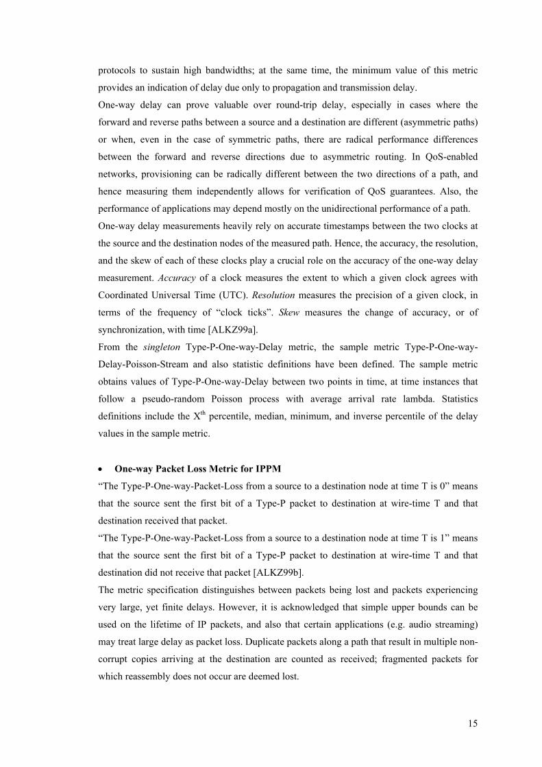
• The “wire arrival time” of a packet P at host H on link L is the first time T at which any

bit of P has appeared at H’s observational position on L.

• The “wire exit time” of a packet P at host H on link L is the first time T at which all the

bits of P have appeared at H’s observational position on L.

Due to the fundamental property of many Internet metrics taking values depending on the type

of IP packets used to make the measurement (e.g. IP-connectivity metric), the generic notion

of “packet of type P” is defined, where in some contexts P will be explicitly defined, partially

defined, or left generic.

Additionally, the framework provides advice on measurement methodologies, on

measurement uncertainties and errors, on composition of metrics, on clock and time resolution

issues, on methods for collecting samples, on measurement calibration and self-consistency

tests, and on the definition of statistical distributions for measurements.

At the time of writing, the IPPM initiative has defined four distinct metrics as well as a bundle

of metrics for measuring connectivity that have advanced along the standards track within the

IETF.

• One-way Delay Metric for IPPM

For a real number dT, “the Type-P-One-way-Delay from a source to a destination node at T is

dT” means that the source sent the first bit of a Type-P packet to the destination at wire-time T

and that destination received the last bit of that packet at wire-time T+dT.

“The Type-P-One-way-Delay from a source to a destination node at T is undefined

(informally, infinite)” means that the source sent the first bit of a Type-P packet to the

destination at wire-time T and that destination did not receive that packet [ALKZ99a].

Main motivation for the definition of the one-way delay metric is the sensitivity of

applications, and especially real-time applications, to large delays and delay variations relative

to some threshold value. Increases in one-way delay also result in difficulty of transport layer

15

protocols to sustain high bandwidths; at the same time, the minimum value of this metric

provides an indication of delay due only to propagation and transmission delay.

One-way delay can prove valuable over round-trip delay, especially in cases where the

forward and reverse paths between a source and a destination are different (asymmetric paths)

or when, even in the case of symmetric paths, there are radical performance differences

between the forward and reverse directions due to asymmetric routing. In QoS-enabled

networks, provisioning can be radically different between the two directions of a path, and

hence measuring them independently allows for verification of QoS guarantees. Also, the

performance of applications may depend mostly on the unidirectional performance of a path.

One-way delay measurements heavily rely on accurate timestamps between the two clocks at

the source and the destination nodes of the measured path. Hence, the accuracy, the resolution,

and the skew of each of these clocks play a crucial role on the accuracy of the one-way delay

measurement. Accuracy of a clock measures the extent to which a given clock agrees with

Coordinated Universal Time (UTC). Resolution measures the precision of a given clock, in

terms of the frequency of “clock ticks”. Skew measures the change of accuracy, or of

synchronization, with time [ALKZ99a].

From the singleton Type-P-One-way-Delay metric, the sample metric Type-P-One-way-

Delay-Poisson-Stream and also statistic definitions have been defined. The sample metric

obtains values of Type-P-One-way-Delay between two points in time, at time instances that

follow a pseudo-random Poisson process with average arrival rate lambda. Statistics

definitions include the Xth percentile, median, minimum, and inverse percentile of the delay

values in the sample metric.

• One-way Packet Loss Metric for IPPM

“The Type-P-One-way-Packet-Loss from a source to a destination node at time T is 0” means

that the source sent the first bit of a Type-P packet to destination at wire-time T and that

destination received that packet.

“The Type-P-One-way-Packet-Loss from a source to a destination node at time T is 1” means

that the source sent the first bit of a Type-P packet to destination at wire-time T and that

destination did not receive that packet [ALKZ99b].

The metric specification distinguishes between packets being lost and packets experiencing

very large, yet finite delays. However, it is acknowledged that simple upper bounds can be

used on the lifetime of IP packets, and also that certain applications (e.g. audio streaming)

may treat large delay as packet loss. Duplicate packets along a path that result in multiple non-

corrupt copies arriving at the destination are counted as received; fragmented packets for

which reassembly does not occur are deemed lost.

16

The definition of the one-way packet loss metric is motivated by the sensitivity of certain

(real-time) applications to excessive loss phenomena, and of transport-layer protocols in

sustaining high bandwidths. Particular importance of one-way packet loss over round-trip loss

is raised due to Internet path asymmetry, queuing asymmetry, and QoS provisioning

phenomena, as well as due to applications’ performance depending mainly on unidirectional

path characteristics.

The sample Type-P-One-way-Packet-Loss-Poisson-Stream metric is derived from the

singleton Type-P-One-way-Packet-Loss metric, following a similar procedure with the Type-

P-One-way-Delay-Poisson-Stream sample metric. Statistic definitions for this sample metric

include the average of all loss values in the stream.

Specific metrics to capture packet loss patterns, such as the frequency and length of loss

phenomena once they start, as well as the spacing between loss periods, have been defined

separately [KoRa02].

• Round-trip Delay Metric for IPPM

For a real number dT, “the Type-P-Round-trip-Delay from a source to a destination node at T

is dT” means that the source sent the first bit of a Type-P packet to the destination at wire-

time T, that destination received that packet, then immediately sent a Type-P packet back to

the source, and that source received the last bit of that packet at wire-time T+dT.

“The Type-P-Round-trip-Delay from a source to a destination node at T is undefined

(informally, infinite)” means that the source sent the first bit of a Type-P packet to the

destination at wire-time T and that (either the destination did not receive the packet, the

destination did not send a Type-P packet in response, or) the source did not receive that

response packet [ALKZ99c].

The round-trip delay metric definition is mainly motivated by the sensitivity of certain

applications to large values of end-to-end delay relative to some threshold value. Also, values

of this metric above the minimum provide an indication of the congestion present in the path.

The round-trip delay metric appeals over its one-way counterpart, due to its ease of

deployment and ease of interpretation properties. It is often possible to perform some form of

round-trip delay measurement without the need of measurement-specific software at the

intended destination (e.g. using ICMP echo or TCP-based methodologies). At the same time,

when round-trip time is the quantity of interest, it can be less accurate to deduce it from one-

way measurements. In measuring round-trip delay there is no synchronisation issue between

the source and destination clocks; rather, there is the easier self-synchronisation issue between

the source clock at the time the test packet is sent and the (same) source clock at the time the

response packet is received. The accuracy of a clock is important only in identifying the time

17

at which a given delay was measured. Accuracy, per se, has no importance to the accuracy of

the measurement of delay [ALKZ99c].

Similar to the Type-P-One-way-Delay-Poisson-Stream sample metric, the sample Type-P-

Round-trip-Delay-Poisson-Stream is derived from the singleton Type-P-Round-trip-Delay

metric. Statistics definitions for the sample Type-P-Round-trip-Delay-Poisson-Stream metric

include the Xth percentile, median, minimum, and inverse percentile of the delay values in the

sample metric.

• IP Packet Delay Variation Metric for IPPM

Type-P-One-way-ipdv is defined for two packets from a source to a destination node selected

by the selection function F, as the difference between the value of the type-P-One-way-delay

from the source to the destination at time T2 and the value of the type-P-One-way-delay from

the source to the destination at time T1. T1 is the wire-time at which the source sent the first

bit of the first packet, and T2 is the wire-time at which the source sent the first bit of the

second packet. This metric is derived from the One-Way-Delay metric.

Therefore, for a real number ddT “The type-P-one-way-ipdv from a source to a destination

node at T1, T2 is ddT” means that the source sent two packets, the first at wire-time T1 (first

bit), and the second at wire-time T2 (first bit), and the packets were received by the

destination at wire-time dT1+T1 (last bit of the first packet), and at wire-time dT2+T2 (last bit

of the second packet), and that dT2-dT1=ddT [DeCh02].

“The type-P-one-way-ipdv from a source to a destination node at T1, T2 is undefined” means

that the source sent the first bit of a packet at T1 and the first bit of a second packet at T2 and

that the destination did not receive one or both packets [DeCh02].

This singleton metric depends on a stream of at least two one-way delay measurements, and

its value is either a real (positive, zero, or negative) or an undefined number of seconds. The

two packets for which the metric is defined can be selected based on some selection function,

such as ‘consecutive Type-P packets within the specified interval’, ‘type-P packets with

specified indices within the specified interval’, ‘type-P packets with the minimum and

maximum one-way-delays within the specified interval’. Being a differential measurement,

this metric is less sensitive to clock synchronization problem; if an error affecting the first

measurement of One-Way-Delay were the same as the one affecting the second measurement,

they will cancel each other when calculating delay variation.

The type-P-One-way-ipdv-Poisson-stream sample metric is derived from the singleton

definition, and statistics to analyse the behaviour of IPDV samples include the distribution of

IPDV values, the Xth percentile, and the inverse percentile. Statistics to compute the variation

of absolute IPDV values and evaluate the behaviour of different scheduling algorithms are

also suggested [JaNP99]. Finally, the peak-to-peak IPDV statistic is defined to compute the

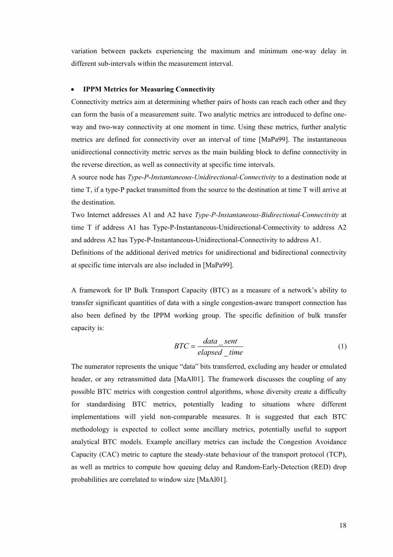
18

variation between packets experiencing the maximum and minimum one-way delay in

different sub-intervals within the measurement interval.

• IPPM Metrics for Measuring Connectivity

Connectivity metrics aim at determining whether pairs of hosts can reach each other and they

can form the basis of a measurement suite. Two analytic metrics are introduced to define one-

way and two-way connectivity at one moment in time. Using these metrics, further analytic

metrics are defined for connectivity over an interval of time [MaPa99]. The instantaneous

unidirectional connectivity metric serves as the main building block to define connectivity in

the reverse direction, as well as connectivity at specific time intervals.

A source node has Type-P-Instantaneous-Unidirectional-Connectivity to a destination node at

time T, if a type-P packet transmitted from the source to the destination at time T will arrive at

the destination.

Two Internet addresses A1 and A2 have Type-P-Instantaneous-Bidirectional-Connectivity at

time T if address A1 has Type-P-Instantaneous-Unidirectional-Connectivity to address A2

and address A2 has Type-P-Instantaneous-Unidirectional-Connectivity to address A1.

Definitions of the additional derived metrics for unidirectional and bidirectional connectivity

at specific time intervals are also included in [MaPa99].

A framework for IP Bulk Transport Capacity (BTC) as a measure of a network’s ability to

transfer significant quantities of data with a single congestion-aware transport connection has

also been defined by the IPPM working group. The specific definition of bulk transfer

capacity is:

_

_data sentBTC

elapsed time= (1)

The numerator represents the unique “data” bits transferred, excluding any header or emulated

header, or any retransmitted data [MaAl01]. The framework discusses the coupling of any

possible BTC metrics with congestion control algorithms, whose diversity create a difficulty

for standardising BTC metrics, potentially leading to situations where different

implementations will yield non-comparable measures. It is suggested that each BTC

methodology is expected to collect some ancillary metrics, potentially useful to support

analytical BTC models. Example ancillary metrics can include the Congestion Avoidance

Capacity (CAC) metric to capture the steady-state behaviour of the transport protocol (TCP),

as well as metrics to compute how queuing delay and Random-Early-Detection (RED) drop

probabilities are correlated to window size [MaAl01].

19

The requirements for a one-way active measurement protocol as well as the use of periodic

sampling streams for network performance measurements have progressed along the IETF

standards track. The measurement protocol requirements include suggestions for functional

and post-processing issues, distribution of results, separation between the session setup and

the actual measurement test process, and support for measurements with different packet types

[ShTe04]. Periodic sampling has been suggested as an alternative to Poisson sampling to

enable simulation of Constant-Bit-Rate (CBR) traffic, and to be applicable to both active and

passive measurement. Sample metrics for periodic streams include the Type-P-One-way-

Delay-Periodic-Stream, which intends to quantify the delays and delay variation as

experienced by multimedia streams of an application [RaGM02].

The One-Way Active Measurement Protocol (OWAMP) has already been submitted as an

IETF draft, and will shortly be considered as a Proposed Standard. This will be a major

deliverable for the IPPM working group, whose standardisation together with the different

metrics definitions can be the corner-stone for wide-spread deployment of one-way and

round-trip performance measurement within network equipment, and across the Internet,

under the umbrella of compatible measurement infrastructures. OWAMP test traffic will

consist of a stream of UDP packets from and to negotiated port numbers, with potentially

nothing static in the packets (negotiated size too). This property should make test traffic hard

to detect and distinguish from operational network traffic, and hence, the possibility of test

traffic being treated differently by network nodes will be kept at a minimum. Two inter-

related protocols have been proposed for control and test traffic. Control will be used to

initiate, start and stop the test sessions and fetch their results, while the test protocol is used to

exchange test packets between two measurement nodes [ShTK05].

It remains to be seen how these efforts towards unambiguous and standardised definitions of

performance metrics and protocol suites will facilitate the wide-spread deployment of

measurement activities within the Internet, essentially creating a measurement plane,

alongside its forwarding and data delivery operations. Coherent measurement support from

different manufacturer equipment, as well as support for inter-domain measurement

operations between Internet Service Providers has a crucial role to play on the successful

evolution of these developments.

2.2.3 ICMP-based Active Measurements

The Internet Control Message Protocol (ICMP) serves the purposes of a gateway or a

destination host occasionally communicating with a source host to report control and error

information in the communication environment, such as errors in datagram processing. ICMP

20

is an integral part of the Internet Protocol, and its implementation is compulsory in every IP

module [Post81].

Even though ICMP messages are encapsulated and sent using IP, ICMP is not considered a

higher layer protocol. The only reason for using IP to deliver ICMP messages is the need for

messages to be able to be travel across several physical networks to reach their final

destination, and therefore they cannot be delivered by the physical transport alone [Come00].

Among the numerous types of ICMP messages that have been standardised and are currently

used across the Internet, the echo request and echo reply messages (Figure 2-1) are deployed

to test destination reachability and status. A host or router sends an ICMP echo request

message to a specified destination; any machine that receives an echo request formulates an

echo reply and returns it to the original sender. The request message contains an optional data

area, and the reply contains an exact copy of this data [Come00].

Figure 2-1: ICMP Echo Request or Reply Message Format

One of the most frequently-used debugging tools that invokes a series of timed ICMP echo

request and reply packets is PING6, first written for UNIX® by Mike Muuss, in December

1983. Sophisticated versions of ping capture responses and provide statistics about datagram

loss, based on the series of ICMP echo messages they generate, and allow users to specify the

length of the data being sent and the time interval between requests. By timing the departure

of the ICMP echo request packets and the arrival of the corresponding ICMP echo replies,

ping can provide information about the Round-Trip Time (RTT) of the path between the

sender and the receiver. The simplicity of ping and its widespread deployment to virtually

every Internet host has encouraged researchers to use it not only as a standalone tool for on-

demand destination reachability tests, but also as the basis to deploy measurement

infrastructures with minimal processing and implementation requirements, to measure certain 6 Mike Muuss named PING after the sound that a sonar makes, inspired by the whole principle of echo-

location. Dave Mills, whose comments were inspirational for the PING author, once suggested that

PING is an acronym for Packet InterNet Groper.

21

performance characteristics across the Internet. Some of these infrastructures now include a

very large number of Internet sites and hence claim that they can capture representative

indications of Internet end-to-end path performance. In the remainder of this section some

major deployments in this area are described.

2.2.3.1 The Ping End-to-end Reporting (PingER) Project

Ping-End-to-end Reporting (PingER) is the name given to the Internet End-to-end

Performance Measurement (IEPM) project to monitor end-to-end performance of Internet

links. The project was initiated at Stanford Liner Accelerator Centre (SLAC) and mainly

included sites involved in the High Energy Nuclear and Particle Physics (HENP) community.

Major motivation behind the project was to understand the present performance and to

allocate resources to optimise performance between laboratories, universities and institutes

collaborating in present and future experiments.

In December 1999 the project consisted of 20 PingER monitoring sites, mainly in the U.S (8),

Europe (7) and Asia (3). Recently, it has been reported that it now includes 35 monitoring

sites in 12 countries that are monitoring hosts across 106 countries in 15 regions [CoLW03,

PiER]. As its name indicates, PingER uses the ping utility to get RTT and loss statistical

summaries across the monitoring sites. It sends 11 pings with a 100-byte payload at 1

second intervals, followed by 10 pings with a 1000-byte payload, also at 1 second intervals.

The first ping is only used to prime name server caches and is then discarded from the

measurement, since it is assumed to be unrepresentatively slow7. The ping default timeout

of 20 seconds is used, since studies on poor links with long delays have shown that less than

0.1 % of packets return after 20 seconds and before 100 seconds. Each set of 10 pings is

called a sample, and each monitoring node-remote node combination a pair [MaCo00a].

Figure 2-2 provides a graphical representation of the PingER architecture. Each of the

monitoring sites chooses a set of remote hosts of interest to them. Additionally, a set of

representative hosts, called beacons, have been chosen for the various regions and they are

monitored by all monitoring-hosts, providing measures for world-wide performance with

respect to the beacons [CoLW03].

7 Studies using UDP echo packets have found that the first packet takes almost 20% longer than

subsequent packets [Horn97].

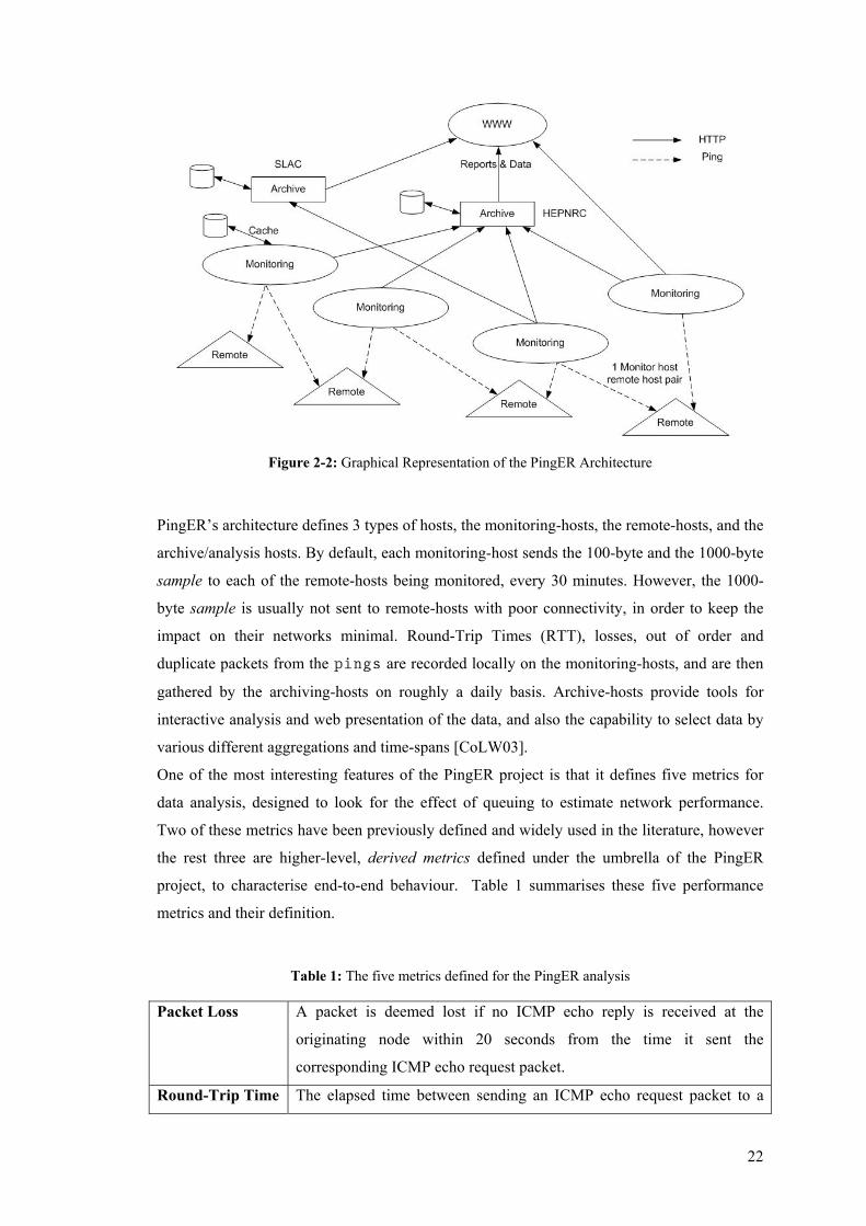
22

Figure 2-2: Graphical Representation of the PingER Architecture

PingER’s architecture defines 3 types of hosts, the monitoring-hosts, the remote-hosts, and the

archive/analysis hosts. By default, each monitoring-host sends the 100-byte and the 1000-byte

sample to each of the remote-hosts being monitored, every 30 minutes. However, the 1000-

byte sample is usually not sent to remote-hosts with poor connectivity, in order to keep the

impact on their networks minimal. Round-Trip Times (RTT), losses, out of order and

duplicate packets from the pings are recorded locally on the monitoring-hosts, and are then

gathered by the archiving-hosts on roughly a daily basis. Archive-hosts provide tools for

interactive analysis and web presentation of the data, and also the capability to select data by

various different aggregations and time-spans [CoLW03].

One of the most interesting features of the PingER project is that it defines five metrics for

data analysis, designed to look for the effect of queuing to estimate network performance.

Two of these metrics have been previously defined and widely used in the literature, however

the rest three are higher-level, derived metrics defined under the umbrella of the PingER

project, to characterise end-to-end behaviour. Table 1 summarises these five performance

metrics and their definition.

Table 1: The five metrics defined for the PingER analysis

Packet Loss A packet is deemed lost if no ICMP echo reply is received at the

originating node within 20 seconds from the time it sent the

corresponding ICMP echo request packet.

Round-Trip Time The elapsed time between sending an ICMP echo request packet to a

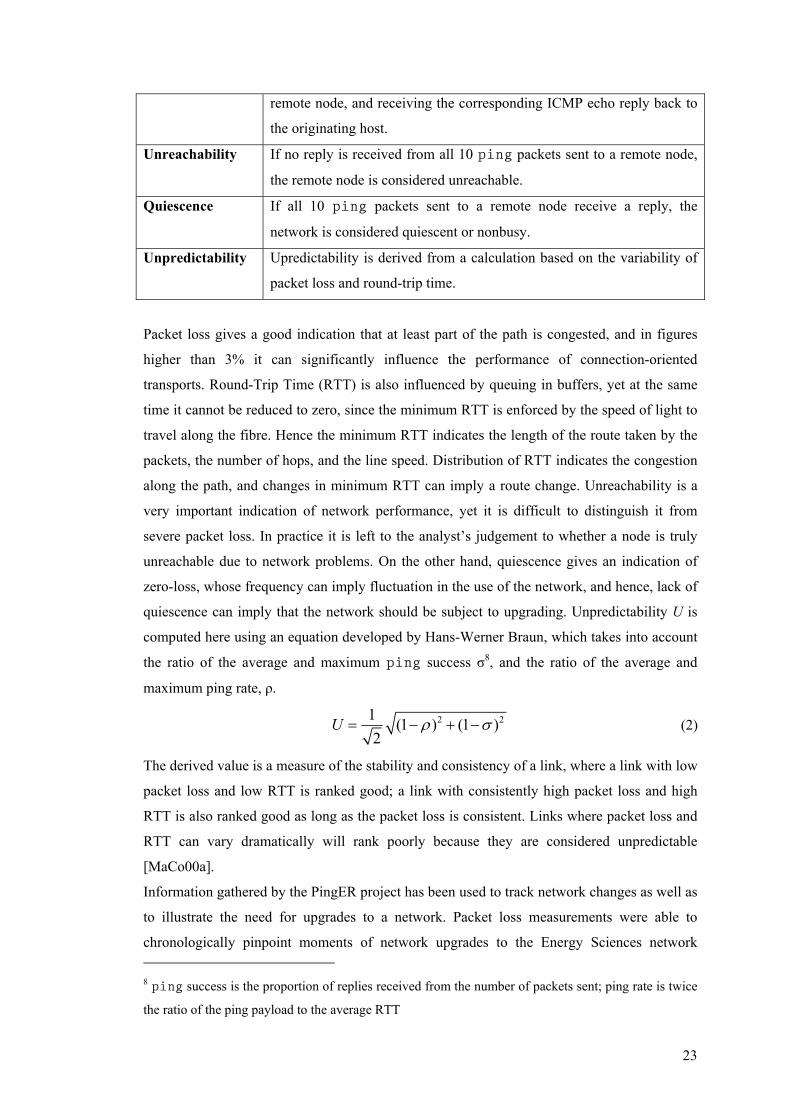
23

remote node, and receiving the corresponding ICMP echo reply back to

the originating host.

Unreachability If no reply is received from all 10 ping packets sent to a remote node,

the remote node is considered unreachable.

Quiescence If all 10 ping packets sent to a remote node receive a reply, the

network is considered quiescent or nonbusy.

Unpredictability Upredictability is derived from a calculation based on the variability of

packet loss and round-trip time.

Packet loss gives a good indication that at least part of the path is congested, and in figures

higher than 3% it can significantly influence the performance of connection-oriented

transports. Round-Trip Time (RTT) is also influenced by queuing in buffers, yet at the same

time it cannot be reduced to zero, since the minimum RTT is enforced by the speed of light to

travel along the fibre. Hence the minimum RTT indicates the length of the route taken by the

packets, the number of hops, and the line speed. Distribution of RTT indicates the congestion

along the path, and changes in minimum RTT can imply a route change. Unreachability is a

very important indication of network performance, yet it is difficult to distinguish it from

severe packet loss. In practice it is left to the analyst’s judgement to whether a node is truly

unreachable due to network problems. On the other hand, quiescence gives an indication of

zero-loss, whose frequency can imply fluctuation in the use of the network, and hence, lack of

quiescence can imply that the network should be subject to upgrading. Unpredictability U is

computed here using an equation developed by Hans-Werner Braun, which takes into account

the ratio of the average and maximum ping success σ8, and the ratio of the average and

maximum ping rate, ρ.

2 21 (1 ) (1 )2

U ρ σ= − + − (2)

The derived value is a measure of the stability and consistency of a link, where a link with low

packet loss and low RTT is ranked good; a link with consistently high packet loss and high

RTT is also ranked good as long as the packet loss is consistent. Links where packet loss and

RTT can vary dramatically will rank poorly because they are considered unpredictable

[MaCo00a].

Information gathered by the PingER project has been used to track network changes as well as

to illustrate the need for upgrades to a network. Packet loss measurements were able to

chronologically pinpoint moments of network upgrades to the Energy Sciences network 8 ping success is the proportion of replies received from the number of packets sent; ping rate is twice

the ratio of the ping payload to the average RTT

24

(ESnet), and also to show reduction in congestion during holiday seasons [MaCo00b]. Based

on presentation of findings revealing a packet loss of around 15% a successful

recommendation was made to increase the bandwidth of the KEK/Tokyo-BINP/Novosibirsk

link from 128 to 512 Kb/s. Following this link update, packet loss was reduced to 0.1%.

PingER has also been used as a troubleshooting tool to discern if a reported problem is

network-related, identify the problem’s timescales, and provide quantitative analysis for ISPs

[CoLW03].

PingER is currently faced with the challenge of discovering whether the ICMP traffic used to

measure end-to-end Internet performance is being treated preferentially in points in the

network. Mainly to identify whether there are pings being blocked or rate limited. Blocking

is relatively easy to detect, while rate limiting is more challenging since there needs to be

some sort of comparable analysis with different types of traffic. Additionally, when blocking

or rate limiting occurs at intermediate ISPs and not at the remote site, then the only feasible

solution is usually to remove the remote host from the monitoring.

Researchers working on PingER are currently trying to maintain, upgrade and expand

deployment of the infrastructure, and also to collect, archive and analyse the monitoring data.

2.2.3.2 The Skitter Project

Skitter is a tool designed and implemented by the Cooperative Association for Internet Data

Analysis (CAIDA) for actively probing the Internet in order to analyse topology and

performance. It measures the forward path and Round-Tip Time (RTT) to a set of destination

hosts, by sending probe packets through the network, without requiring any configuration or

cooperation from the remote sites on its target list. CAIDA encourages site administrators to

be receptive to Skitter measurements at low frequency, since these efforts are intended to help

users, providers and researchers to understand the complexities of current and future Internet

[Skit]. CAIDA started creating three main categories of destinations lists for the Skitter

project, for web servers, IPv4 space, and DNS clients. The web servers list was created from a

variety of log file sources, and by using in-addr.arpa to get domain names and then adding

www to the beginning of the domain names to test for existence of web servers. The IPv4

space list was developed to try to cover one responding destination for each reachable 256-

adresses segment (/24) of IPv4 address space. The DNS clients list was created to study the

connectivity and performance of root DNS servers, by collecting IP addresses seen in passive

data from root servers, and selecting one IP address per routable prefix [HFMC01].

The main objectives of the project are to collect path and RTT data, to acquire infrastructure-

wide global connectivity information, to analyse the visibility and frequency of IP routing

changes, and to visualise network-wide IP connectivity. RTT information is gathered in a

manner similar to traceroute, by incrementing the Time-To-Live (TTL) field of each

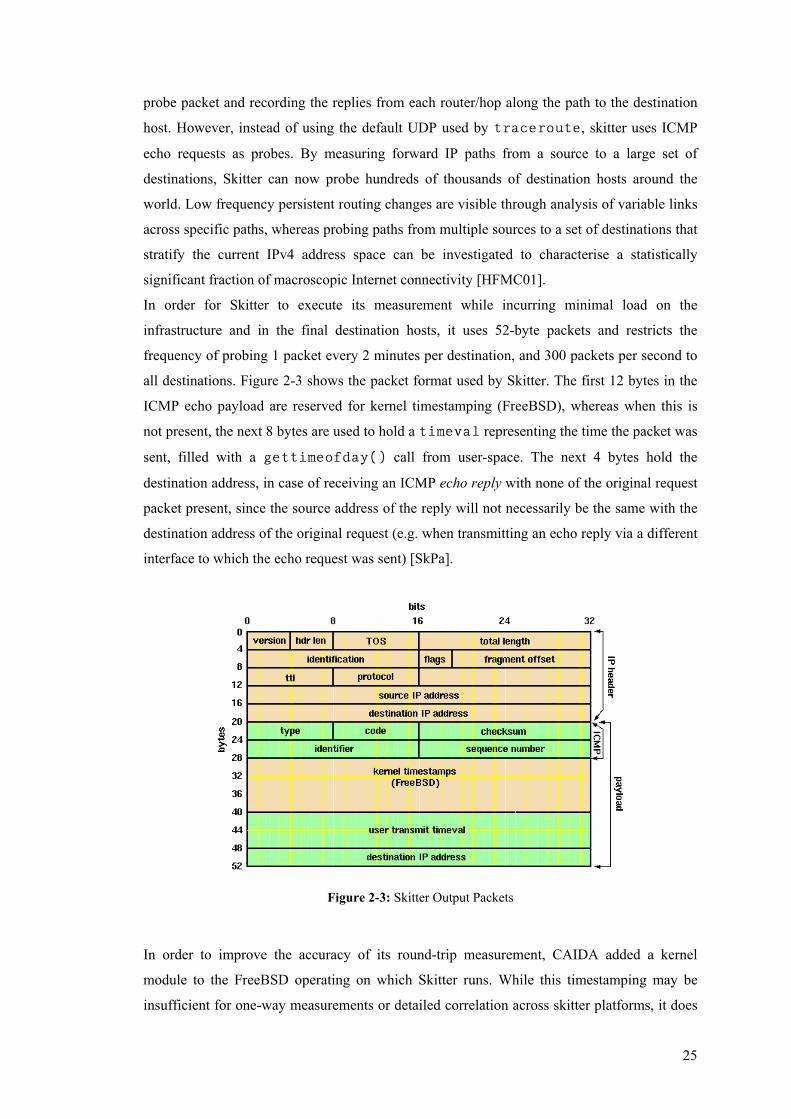
25

probe packet and recording the replies from each router/hop along the path to the destination

host. However, instead of using the default UDP used by traceroute, skitter uses ICMP

echo requests as probes. By measuring forward IP paths from a source to a large set of

destinations, Skitter can now probe hundreds of thousands of destination hosts around the

world. Low frequency persistent routing changes are visible through analysis of variable links

across specific paths, whereas probing paths from multiple sources to a set of destinations that

stratify the current IPv4 address space can be investigated to characterise a statistically

significant fraction of macroscopic Internet connectivity [HFMC01].

In order for Skitter to execute its measurement while incurring minimal load on the

infrastructure and in the final destination hosts, it uses 52-byte packets and restricts the

frequency of probing 1 packet every 2 minutes per destination, and 300 packets per second to

all destinations. Figure 2-3 shows the packet format used by Skitter. The first 12 bytes in the

ICMP echo payload are reserved for kernel timestamping (FreeBSD), whereas when this is

not present, the next 8 bytes are used to hold a timeval representing the time the packet was

sent, filled with a gettimeofday() call from user-space. The next 4 bytes hold the

destination address, in case of receiving an ICMP echo reply with none of the original request

packet present, since the source address of the reply will not necessarily be the same with the

destination address of the original request (e.g. when transmitting an echo reply via a different

interface to which the echo request was sent) [SkPa].

Figure 2-3: Skitter Output Packets

In order to improve the accuracy of its round-trip measurement, CAIDA added a kernel

module to the FreeBSD operating on which Skitter runs. While this timestamping may be

insufficient for one-way measurements or detailed correlation across skitter platforms, it does

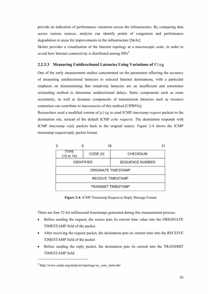
26

provide an indication of performance variations across the infrastructure. By comparing data

across various sources, analysts can identify points of congestion and performance

degradation or areas for improvements in the infrastructure [SkAr].

Skitter provides a visualisation of the Internet topology at a macroscopic scale, in order to

reveal how Internet connectivity is distributed among ISPs9.

2.2.3.3 Measuring Unidirectional Latencies Using Variations of Ping

One of the early measurement studies concentrated on the parameters affecting the accuracy

of measuring unidirectional latencies to selected Internet destinations, with a particular

emphasis on demonstrating that round-trip latencies are an insufficient and sometimes

misleading method to determine unidirectional delays. Static components such as route

asymmetry, as well as dynamic components of transmission latencies such as resource

contention can contribute to inaccuracies of this method [ClPB93a].

Researchers used a modified version of ping to send ICMP timestamp request packets to the

destination site, instead of the default ICMP echo requests. The destination responds with

ICMP timestamp reply packets back to the original source. Figure 2-4 shows the ICMP

timestamp request/reply packet format.

Figure 2-4: ICMP Timestamp Request or Reply Message Format

There are four 32-bit millisecond timestamps generated during this measurement process:

• Before sending the request, the source puts its current time value into the ORIGINATE

TIMESTAMP field of the packet.

• After receiving the request packet, the destination puts its current time into the RECEIVE

TIMESTAMP field of the packet

• Before sending the reply packet, the destination puts its current into the TRANSMIT

TIMESTAMP field. 9 http://www.caida.org/analysis/topology/as_core_network/

27

• After receiving the reply packet, the source calculates its current time and has all four

time values needed for the one-way latency calculation.

The first and last of these four timestamps correspond to those used by the ICMP echo

request/reply packets. The difference between successive timestamps (second-first, fourth-

third) can be used as indicators of the outbound and return latencies, respectively.

The researchers emphasised that these differences are not necessarily indicative of the delays

across the network, but rather of clock states, together with their characteristic drift and

asynchronicity due to local clock adjustment methods to compensate for such drifts

[ClPB93a]. However, since the concentration of this measurement study was on the

fluctuations of unidirectional latencies, rather than their absolute values, tight synchronisation

of end-system clocks was not a primary concern. The core of the hypothesis under

investigation was that the variance in latencies on the two opposing paths of a connection is

often significant. The effects of asymmetric delay variance proved to be one to two orders of

magnitude larger (as much as one second in some cases) than the effects of clock

synchronisation or internal machine clock accuracies. Consistency among a continual series of

measurements was hence more important than the accuracy of single measurements of

outgoing and return delays.

The measurements consisted of simultaneous 96-hour probing of four Internet paths from US

to US, Europe and Asia, using bursts of 20 ICMP timestamp request packets10.

Results of this study reported remarkable variances in the differences between the measured

timestamps on the two paths, sometimes sustained for significant periods, often simultaneous

with increased round-trip delays [ClPB93a].

2.2.4 UDP and TCP-based Active Measurements

In the TCP/IP Protocol suite, the User Datagram Protocol (UDP) and the Transmission

Control Protocol (TCP) provide the two fundamental packetisation (transport) mechanisms

used to encapsulate all application-level data exchanged over the Internet. UDP provides an

unreliable connectionless delivery service that uses IP to carry stateless datagrams and adds

the ability to distinguish among multiple destinations within a given host computer. On the

other hand, TCP uses the connection as its fundamental abstraction to provide for a reliable

stream delivery, and an error detection and recovery mechanism transparently to the

application, using the positive acknowledgment with retransmission technique [Come00].

10 Each burst sent a new ICMP timestamp request packet upon reception of an ICMP timestamp reply

from a specified destination

28

Numerous infrastructures exploit either of these transport protocols to measure the

performance between two instrumented points in the Internet. Transport-based measurement

processes do not have the advantage of using some universally applicable mechanism11 that

would allow them to measure the properties of a path to potentially any network node without

being explicitly part of the measurement infrastructure; nevertheless, the test traffic has the

same characteristics with a (large or small) portion of the actual network traffic and therefore

an increasing probability of eliciting an identical network response.

UDP has been more frequently-used to carry the measurement traffic since it provides an

application-layer process with greater control over the packetisation of the test traffic. On the

other hand, the majority of traffic has been and still is carried over TCP [ClMT98, FoKM04],

and hence TCP-based measurement results can be far more representative of the performance

experienced by the operational Internet traffic. However, TCP implementations are governed

by protocol-internal algorithms, giving less control over the packetisation of the test traffic to

the measurement.

Both UDP and TCP-based active measurements can provide insight on the unidirectional path

properties and discover interesting and complicated pathologies of Internet paths.

2.2.4.1 RIPE NCC TTM Project

The RIPE NCC (Réseaux IP Européens Network Coordination Centre) is one of the four

Regional Internet Registries (RIR)s and it was established as a not-for-profit membership

organisation to provide services for the benefit of IP-based network operators in Europe and

surrounding areas.

The Test Traffic Measurements (TTM) Project has been provided by RIPE NCC as a regular

active measurements service for Internet Service Providers (ISPs), and its main goal is to

conduct performance measurements according to well-defined and scientifically defendable

standards, by implementing numerous metrics defined within IETF’s IPPM Working Group

(section 2.2.2). TTM uses dedicated measurement devices (Test Boxes) to measure

connectivity parameters between each site and the rest of the Internet, in particular routing

vectors, one-way delay and packet loss, Inter-Packet Delay Variation (IPDV), and bandwidth,

with additional parameters being developed [RIPE].

The main design objective of the TTM project is to concentrate on one-way measurements in

order to find effects that occur in only one direction, and to overpass the uncertainties imposed

by the increasing asymmetric routing in the Internet. The use of active techniques to generate

their own test traffic has been preferred in order to remove any privacy concerns related to

snooping customer traffic, and at the same time to maintain better control of the measurement

11 For example, similar to the IMCP echo responder implemented on all modern hosts

29

data. Additionally, the generated measurement traffic should resemble ‘real’ traffic as much as

possible, so that concerns of preferential treatment of measurement traffic are minimised. Use

of ICMP-based techniques was therefore rejected, since network nodes treat such traffic

differently from UDP or TCP traffic [GeGK01]. The measurement traffic consists of UDP

packets12 that carry a 100-byte UDP payload, which is the TTM Type-P packet definition

[DoGW01]. TCP streams have also planned to form part of the test-traffic at later stages of the

project [UiKo97]. Independently measuring inter-provider networks’ performance based on

standardised metrics allows RIPE to use TTM results to verify service-level agreements.

Figure 2-5 gives an overview of the RIPE Measurement setup. A test box is installed near a

border router of an ISP (ideally, 0 hops from a boarder router) and exchanges measurement

data with other test boxes installed at equivalent locations within different provider networks.

In order to measure one-way delay packets are timestamped before departing the ‘source’ test

box and upon arrival at the ‘destination’ test box, hence, the network transit time is provided

by subtracting the two timestamps. One-way packet loss is measured by keeping packet

counters of departing packets at the originating test box and then computing the fraction of

packets arrived at the ‘destination’ test box. IPDV of two consecutive packets is measured as

the difference of the one-way delay that each packet experienced between the two test boxes.

Routing vectors are computed as being the paths between the test boxes, and are determined

by the traceroute program. While waiting for IPPM to define a standard for bandwidth

measurements, RIPE have integrated into their test boxes a number of existing tools to

measure capacity or raw bandwidth. These are either RTT-based or packet-dispersion based

tools [AlCK02].

Machines at RIPE NCC collect measurement information from the different text boxes,

synthesise the properties of the measurement flows, and then present performance information

as plots and tables of results. At the same time, these machines control the experiments by

sending the necessary configuration data to the test boxes, they start and stop the measurement

processes, and they act as a repository for the measurement software. The destinations as well

as the frequency of the test-traffic are centrally configured, and the sending processes

maintain a randomised interval between consecutive packets according to a Poisson

distribution [GeGK01].

12 Test traffic packets are destined to UDP port 6000.

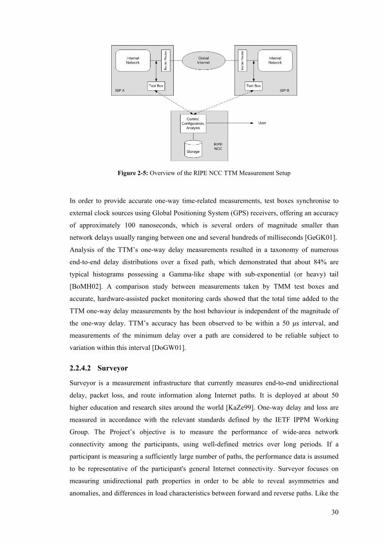
30

Figure 2-5: Overview of the RIPE NCC TTM Measurement Setup

In order to provide accurate one-way time-related measurements, test boxes synchronise to

external clock sources using Global Positioning System (GPS) receivers, offering an accuracy

of approximately 100 nanoseconds, which is several orders of magnitude smaller than

network delays usually ranging between one and several hundreds of milliseconds [GeGK01].

Analysis of the TTM’s one-way delay measurements resulted in a taxonomy of numerous

end-to-end delay distributions over a fixed path, which demonstrated that about 84% are

typical histograms possessing a Gamma-like shape with sub-exponential (or heavy) tail

[BoMH02]. A comparison study between measurements taken by TMM test boxes and

accurate, hardware-assisted packet monitoring cards showed that the total time added to the

TTM one-way delay measurements by the host behaviour is independent of the magnitude of

the one-way delay. TTM’s accuracy has been observed to be within a 50 µs interval, and

measurements of the minimum delay over a path are considered to be reliable subject to

variation within this interval [DoGW01].

2.2.4.2 Surveyor

Surveyor is a measurement infrastructure that currently measures end-to-end unidirectional

delay, packet loss, and route information along Internet paths. It is deployed at about 50

higher education and research sites around the world [KaZe99]. One-way delay and loss are

measured in accordance with the relevant standards defined by the IETF IPPM Working

Group. The Project’s objective is to measure the performance of wide-area network

connectivity among the participants, using well-defined metrics over long periods. If a

participant is measuring a sufficiently large number of paths, the performance data is assumed

to be representative of the participant's general Internet connectivity. Surveyor focuses on

measuring unidirectional path properties in order to be able to reveal asymmetries and

anomalies, and differences in load characteristics between forward and reverse paths. Like the

31

RIPE NCC TTM project described in the previous section, Surveyor also use dedicated

measurement machines at participating sites to ensure that each machine is uniform and runs

at controlled load, thus avoiding ‘noise’ in the measurement and maintaining high timestamp

accuracy. Modifications to the network drivers of the measurement machines allow

timestamps to be taken from within the kernel code, enabling accurate13 measurement even at

high load [KaZe99]. Clock synchronisation for the one-way measurements is achieved by

using Global Positioning System (GPS) receivers at the measurement machines. Surveyor

performs continuous measurements to identify trends on the traffic performance that can then

be exploited to provide information on provisioning, capacity planning and network

engineering, and at the same time to reduce the possibility of not revealing periodic network

events.

One-way delay and packet loss are measured using the same stream of active test traffic,

consisting of 40-byte UDP packets that carry a 12-byte payload, which follows a Poisson

process sending on average 2 packets per second. The receiving machine maintains

knowledge of the test schedules, and hence it can compute packets that do not arrive. A Packet

is deemed lost if it does not arrive within 10 seconds. Route information is gathered for the

same paths as delay and loss using a modified version of traceroute scheduled to run

once every 10 minutes. Apart from the measurement machines, the Surveyor infrastructure

employs two other components, a central database and a data analysis web server. The

database periodically polls the measurement machines and collects performance data, and the

web server generates 24-hour summary statistics and plots for each path [KaZe99].

Surveyor’s measurements have been used to reveal routing changes along instrumented paths,

asymmetries in routing between participating sites, as well as effects of network infrastructure

upgrades and connectivity testing. Monthly reports have shown overall low levels of packet

loss mainly between academic and research institutions across the U.S. and Europe, but also

loss asymmetries between the forward and reverse directions especially of paths experiencing

overall greater than 1% loss. Asymmetries in propagation delays between measured paths

were reported to be relatively small over a monthly period, yet a small percentage of paths

experienced asymmetric delays by more than 5 milliseconds over specific days.

13 Performance metrics are defined in terms of ‘wire-time’, which is the time between the first bit of a

packet is transmitted from a source and the time the last bit of the packet is received by the network

interface of a destination. On the other hand, timestamps taken by measurement software at ‘host-time’

differ from wire-time because of hardware and software overhead. Hence, the accuracy of a

measurement system largely depends on its ability to provide a minimum and consistent difference

between these two notions of time, independently of the measurement load.

32

Empirical data from the Surveyor infrastructure has been used to demonstrate the existence of

distinct phases in congestion events, separating them in queue build-up, packet dropping, and

TCP reaction phases [GaBa02]. Also, a study that compared measurement results from the

Surveyor infrastructure with application-level measurements concluded that the network-level

performance information does not match an application’s view of performance over the same

Internet paths. Although an approximation of the network performance can be provided,

applications with higher packet rates than the Surveyor probes can experience a much worse

performance than that observed by the measurement infrastructure [ClJe99].

2.2.4.3 AT&T Tier 1 Active Measurements

As it will be discussed later in this chapter, operators take advantage of having administrative

access to large networks to deploy monitoring infrastructures to measure performance

properties of their actual network traffic. Active measurements are not usually employed

within single ISP networks to assess or to resolve problems in an operational setting.

However, researchers at AT&T Laboratories developed and used an active monitoring system

in the AT&T backbone to provide a comprehensive view of network performance and to

complement traditional element-level monitoring, forming an integral part of the operator’s

network management setup. This system continuously monitors the path-level performance of

a Tier-1 backbone network topology and is designed to produce operational level alerts and

data, providing the basis for proactive issue resolution. The main motivation behind the

deployment of an active measurement system lies on its ability to estimate packet transfer

performance during congestion and recovery events, which is especially valuable for real-

time, interactive applications and Voice over IP (VoIP) [CiMR03].

Researchers designed two test sequences of probe packets, a periodic [RaGM02] and a

Poisson [PaAM98], to run in parallel within a test cycle between pairs of measurement servers

across 18 major AT&T networking centres. The Poisson probe sequence running throughout

the test cycle is able to characterise events that the periodic probe could miss out, even if they

occurred in every test cycle. Continuous measurement is performed by dividing each 24-hour

day into 96 15-minutes-long test cycles. Each Poisson probe sequence sends 278-byte UDP

packets throughout a test cycle with an average inter-arrival time of 3.3 seconds. One-minute

long periodic probe sequences are started at random within every 15-minute test cycle and

send 60-byte UDP packets between pairs of measurement servers, maintaining a 20

milliseconds interval between successive packets. The tests are used to measure a variety of

performance metrics including delay, packet loss and re-ordering, and delay variation, across

the instrumented backbone paths. Additionally, a traceroute is performed prior to each

test cycle in order to assess the stability and possible asymmetries for each path.

33

2.2.4.4 End-to-end Internet Traffic Analysis

Vern Paxson’s work in mid 1990s was followed by an explosion of Internet measurements

research and played a significant role on the ongoing (if not increasing) popularity of the

subject within the overall networking research community. The main focus of this work was

on the empirical measurement and validation of the overall behaviour of the Internet traffic, as

this is derived by two major streams, namely end-to-end routing behaviour and end-to-end

Internet packet dynamics.

The end-to-end routing study was conducted by recruiting approximately 40 Internet sites to

periodically run a network probe daemon and measure the route to another participating site

using the traceroute utility. The Network Probe Daemon (NPD) is a framework for

probing paths through the Internet by tracing the corresponding routes to the paths, and by

sending TCP along the paths and tracing the arrivals of both the packets and the

acknowledgments [Paxs97b]. Two scheduled sets of measurements resulted in a large dataset

of approximately 40000 traceroutes to be collected and analysed to report a

comprehensive set of routing pathologies. Persistent and temporary routing loops, erroneous

routing, altered connectivity between autonomous Systems (AS), infrastructure failures,

temporary outages, and time-of-day routing patterns were among the most notable routing

pathology categories that were studied, and revealed the overall likelihood of each situation

occurring, together with estimates of the trend to improvement or otherwise. The overall

likelihood of encountering a major routing pathology was reported to have doubled between

the end of 1994 and the end of 1995, rising from 1.5% to 3.4%. Routing stability and

symmetry were also investigated to report that two thirds of the studied paths experienced

stable routes persisting for days or weeks, and that the majority of asymmetries were confined

to a single hop [Paxs96].

The end-to-end packet dynamics study developed characterisations of the dynamics of

Internet packet loss and delay, and examined network pathologies such as out-of-order packet

delivery, packet replication and packet corruption. For the purposes of this study, the

measurement probes consisted of unidirectional bulk TCP transfers of 100-KB files over

different Internet paths. The use of TCP was mainly motivated by its dominant presence in the

Internet, and its congestion control properties that adapt the probe transmission rate to the

current network conditions. Consequently, the end-to-end performance observed by TCP

transfers closely matches the service Internet users receive from the network, in contrast to

echo-based techniques (such as UDP or ICMP) whose sending rate is relatively random and

cannot be statically defined to be optimal for an Internet path. An inherent part of the study

was the development of an analysis tool to account for the details of the numerous TCP

implementations and separate their effects from the true networking effects [Paxs97b].

34

Approximately 20,000 bulk TCP transfers between 35 Internet sites were analysed to report

the relative prevalence and great asymmetry of packet re-ordering in the Internet, dominant in

data packets (and not to acknowledgment packets), and the frequent presence of packet

corruption. Packet loss was found to sometimes be completely independent between the

forward and reverse direction of the paths. Loss patterns of acknowledgment packets differed

significantly from those of data packets, reflecting the fact that the acknowledgment stream

does not adapt as much to the current network conditions, and thus experiences loss even

though it is a much lighter load compared to the data packet stream. Packet delay analysis

reported only small timing compression events mainly for acknowledgment packets, with a

mean number of 2 occurrences in approximately half of the instrumented connections,

whereas in the data path this phenomenon was even rarer, having minor impact [Paxs97a].

The measurement data gathered was also used to empirically assess the impact of

unsynchronised clocks on the accuracy of wide-area network measurements, to develop

algorithms for detecting clock adjustments and relative clock skew, and possible systematic

errors. While these algorithms require heuristics to minimise inaccuracies they check for self-

consistency in the measurement process and provide for calibration of the results [Paxs98a].

• The National Internet Measurement Infrastructure (NIMI)

As a natural evolution of the end-to-end Internet measurement study, a measurement

infrastructure was proposed and started being incrementally deployed, in which a collection of

measurement platforms cooperatively measures the properties of Internet paths and

Autonomous Systems (AS). The National Internet Measurement Infrastructure (NIMI) was

initiated by the National Science Foundation (NSF) and is currently funded by the Defence

Advanced Research Projects Agency (DARPA)14. The main objective of NIMI is the

development of a generalised architecture for a scalable measurement infrastructure, rather

than performing a specific set of measurements for specific analysis goals [PaMA98].

NIMI’s design goals and constraints are for the infrastructure to work on an administratively

diverse environment and in parallel to the commercial Internet, where several entities have

significant business considerations. Hence, scalability is one of the fundamental properties for

the infrastructure in order to be able to adapt with the increasing population of the Internet,

rather than only be restrictively deployable on a small scale. At the same time, security is

another major requirement, and therefore, communication between NIMI components is

encrypted and authenticated using public key credentials, and each probe is configured to

authorise particular sets of operations per credential.

14 http://www.ncne.org/nimi/

35

From a core measurement-oriented perspective, NIMI is designed to support a wide range of

measurements by adopting the notion of measurement modules, so that various specific

measurement functions can be embraced under the umbrella of an overall engine with

carefully specified interfaces. Currently, together with traceroute, mtrace for multicast

route measurements, treno and cap/capd for bulk transfer capacity, and zing for round-

trip delay and loss measurements, are some of the deployed measurement modules. Adding a

new measurement tool as a module simply requires generating a wrapper for the tool and

propagating both the tool and the wrapper to all NIMI probes [PaAM00]. Active

measurements are preferred primarily because NIMI focuses on wide-area performance

measurements, but also because of privacy and security concerns raised by passive

measurements.

NIMI has the potential of eventually becoming one of the most successful measurement

infrastructures, massively deployed across the Internet. Research is currently focusing on

overcoming systems and networks’ heterogeneities and on providing a distributed

measurement environment who’s Measurement Clients (MC) could potentially run even on

commodity end-systems. In this respect, the specification of a solid architectural framework

with standardised methods for site participation and access control is vital. Remote error

handling, associated measurement grouping, public key distribution, transparent and

automated installation, systems’ clocks, and efficient usage of systems’ resources are among

the most important issues under investigation [PaAM00].

2.2.5 The Active Measurement Project (AMP) and the Internet

Performance Measurement Protocol (IPMP)

The Active Measurement Project (AMP) was initiated at the National Laboratory for Applied

Network Research (NLANR) in 1998 with a focus at conducting site-to-site active

measurements and analyses between campuses connected by high performance networks.

Currently, there are approximately 150 AMP monitors deployed across High Performance

Connection (HPC) sites in the U.S. and internationally15. Across all participating sites, Round-

Trip Time (RTT), packet loss, topology, and user and event-driven throughput are measured.

Each of the AMP monitors sends a single, 64-byte ICMP packet to each of the others every

minute, and records the time until a reply is received, or a loss if no reply is received.

Additionally, the route to each other monitor is recorded using traceroute, every 10

minutes. Throughput tests can be run between any pair of the monitors using a web-based

throughput test request, able to measure bulk TCP and UDP data transfer, and treno

15 http://watt.nlanr.net//

36

throughput [McBr01]. Due to their high cost in terms of network traffic, throughput tests are

only run on-demand and are not scheduled by default.

AMP monitors conduct measurements independently and the collected data is sent to a central

site for processing and web-publication. Due to the continuous nature of the measurements

and the lack of an end-time at which to send data for central processing, AMP designers

developed an active mirror system to update the published results within minutes, and give a

near-real-time nature to the overall infrastructure [McBB00].

More recently, AMP started collecting IPv6 performance information between a mesh of

twelve active monitors with an aim to assess the infrastructure improvements to the IPv6

component of HPC networks, relative to the performance seen by IPv4 paths. It has been

observed that a general characteristic of IPv6 paths is that they experience a larger delay,

delay variation, and packet loss compared to IPv4 paths, a characteristic that is mainly

attributed to IPv6 tunnelled paths following a less-than optimal physical path. However,

continuous improvements are seen to IPv6 paths as IPv6-in-IPv4 tunnels are replaced with

native IPv6 paths and the IPv6 forwarding capability of routers in the path is improved16.

At the early days of the project, a variety of active measurements techniques were deployed,

using ICMP as well as TCP and UDP-based measurement processes to measure a variety of

performance characteristics over the AMP infrastructure. This attribute gave some uniqueness

to AMP, in relation to other active measurements infrastructures that either focused on

Round-trip (ICMP-based) or on one-way (UDP/TCP-based) performance measurements.

What made AMP an even more unique project over the years though was the decision to

specify a new measurement protocol to be used as an alternative to ICMP across the AMP

infrastructure. The IP Measurement Protocol (IPMP) has been proposed as a customised

active measurement protocol to contain facilities to carry timestamps and path information,

with a view of being potentially implemented in the forwarding path of routers [McBr00]. The

protocol is based on an echo request and reply packet exchange for measuring packet delay

and associated path metrics, and is very similar to the technique ping uses with the ICMP echo

capabilities. IPMP is carried directly inside of an IP datagram in order to make an echo packet

obvious to the routers along a measurement path [LuMB01]. Similarly to the ICMP echo

request and reply messages, the IPMP echo reply message has been designed so that an echo

host constructs it with minimal modifications to the echo request packet. Figure 2-6 shows the

IPMP echo packet format.

16 http://watt.nlanr.net/IPv6/

37

Figure 2-6: The IPMP Echo Packet

The packet format provides some sophisticated processing capabilities including the selection

of certain processing queues in routers that implement priority queuing. Through the Protocol

Queue field the packet identifies how it should be prioritised, e.g. by setting it to

IPROTO_TCP the echo packet requests to be prioritised as a TCP packet. Whether a packet is

an echo request or an echo response is identified by the Type field. The allocation of the filler,

type, returned TTL, and return type bytes allows the echo request packet to be transformed

into an echo response by swapping the two 16-bit words in place17, without requiring

checksum re-calculation. The Path Pointer field specifies where in the packet the next Path

Record should be inserted, providing direct access. The Source and Destination Port Queue

fields can be used to queue or filter the packet according to a more synthetic tuple than the

simple Protocol Queue field [LuMc02].

When network nodes that support IPMP send, forward, or receive an echo packet, they insert

their forwarding address and a 64-bit departure or arrival timestamp, in the form of a Path

Record (Figure 2-7).

Figure 2-7: Path Record Format

A host can perform an echo measurement by creating an echo request packet, addressing it to

the target host, and sending it onto the network. IPMP-capable routers along the path can

17 The Returned TTL is set to zero in the echo request packet. If it is updated by the target host, the

IPMP checksum can be updated incrementally [Rijs94].

38

insert their path records signifying the time the packet arrived on their interface. Non-IPMP-

capable routers simply forward the packet. Upon arrival at the target echo host, another path

record is inserted, and the packet is transformed into an echo reply message and routed back

to the originating host.

Using this procedure, IPMP can measure end-to-end and intermediate one-way delay in both

the forward and reverse directions, and also deduce path length in hops in each direction.

Increasing the size of the packet by the size of a path record is an issue, but since IPMP does

not carry additional payload data, even the 576 bytes minimum MTU supported by IPv4

allows for 45 path records to be stored in an echo packet.

IPMP seeks the cooperation of the routers along an instrumented path and it maintains a

format that can potentially be processed in an efficient manner at routers’ line cards. If it is

only supported by instrumented end-systems it can provide similar capabilities to the ICMP

timestamp request and reply messages. Additional IPMP message types provide a mechanism

for time synchronisation information to be collected from hosts and routers, in order to

estimate the accuracy of their individual clocks [LuMB01]. IPMP is now in its fourth version

as a work-in-progress document within the IETF, and might soon be proposed for a

standard18.

It is the intention of AMP researchers to gradually replace the ICMP delay and loss

measurements that are currently collected with IPMP and further exploit the protocol’s

capabilities. Experiments have been conducted to compare the differences in round-trip delay

and loss measurements between the ICMP and the IPMP echo protocols within the AMP

infrastructure. Preliminary results revealed that the majority of measured paths showed no

bias, yet 8% of the paths returned smaller and 10% of the paths larger average delays when

measured with IPMP echo packets. However, the differences between the average delays were

more significant when IPMP echo packets reported smaller values than ICMP, leaving only a

0.006% of paths to show at least a 10 millisecond larger average delay with IPMP than with

ICMP echo packets. Packet loss indications were very similar between the two protocols, not

revealing that anyone was more or less likely to lose packets than the other [LuMc02].

18 http://watt.nlanr.net/AMP/IPMP/draft-mcgregor-ipmp-04.txt

39

2.2.6 Bandwidth Estimation

Bandwidth estimation is a special case of active measurements, where synthetic traffic is

injected into the network to try and characterise the amount of data that can be transferred by

the infrastructure per unit of time. The area is lately seeing an increasing popularity and is

sometimes considered to be exhibiting distinct characteristics from other measurement work19.

This is not due to the use of specific infrastructures or certain protocols during the

measurement process (as it was the case with most of the previous sections of this chapter),

but mainly due to the focus being on the measurement practices and methodologies, and on

assumptions (or lack of) that will produce accurate and unbiased results. Bandwidth is a

fundamental property of a network connection, and producing a representative estimation of

its metrics using raw packet values, requires an intensive investigation of measurement

strategies that can minimise the heuristics and assumptions during the measurement process,

as well as during the measurement analysis. This section briefly discusses the major issues

and outlines the main measurement strategies in bandwidth estimation, which still remains a

relatively new (sub-)area of network measurements research. Bandwidth measurements are

viewed as complementary active probing techniques, yet the detailed analysis of the origins,

theory, applications and implications of bandwidth estimation is beyond the scope of this

thesis.

Within the data networks context, the term bandwidth quantifies the data rate that a network

link or path can transfer. Three major metrics have been defined in the literature to identify

different aspects of bandwidth. The capacity or bottleneck bandwidth of a link or path sets the

upper limit on how quickly the network can deliver the sender’s data to the receiver. The

capacity C of an H-hop end-to-end path is the maximum IP layer rate that the path can transfer

from source to sink, and it depends on the underlying transmission technology and

propagation medium [PrMD03]. The end-to-end capacity is determined by the minimum link

capacity, i.e. the slowest forwarding element (narrow link) in the end-to-end chain that

comprises the path.

0...

min ii HC C

== (3)

Bottleneck bandwidth gives an upper bound on how fast a connection can possibly transmit

data [Paxs97a]. The available bandwidth of a link relates to its ‘spare’ capacity during a

certain time period, and relates not only on the underlying medium, but also on the traffic

load. At any specific time instant, a link is either transmitting a packet at full link capacity or

19 The First Bandwidth Estimation (BEst) workshop was organised by IETF’s Internet Measurement

Research Group (IMRG), CAIDA, and the US Department of Energy (DoE) in December 2003

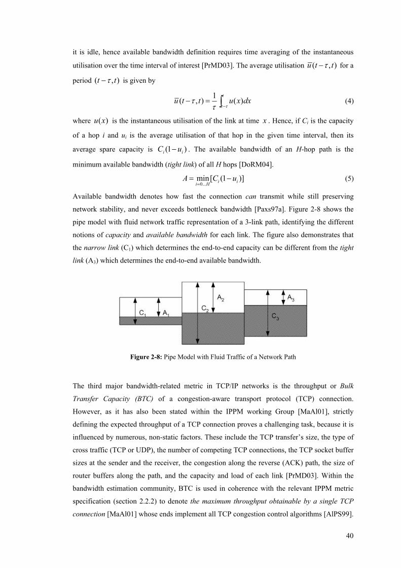
40

it is idle, hence available bandwidth definition requires time averaging of the instantaneous

utilisation over the time interval of interest [PrMD03]. The average utilisation ),( ttu τ− for a

period ),( tt τ− is given by

1( , ) ( )

t

tu t t u x dx

ττ

τ −− = ∫ (4)

where )(xu is the instantaneous utilisation of the link at time x . Hence, if Ci is the capacity

of a hop i and ui is the average utilisation of that hop in the given time interval, then its

average spare capacity is )1( ii uC − . The available bandwidth of an H-hop path is the

minimum available bandwidth (tight link) of all H hops [DoRM04].

0...

min[ (1 )]i ii HA C u

== − (5)

Available bandwidth denotes how fast the connection can transmit while still preserving

network stability, and never exceeds bottleneck bandwidth [Paxs97a]. Figure 2-8 shows the

pipe model with fluid network traffic representation of a 3-link path, identifying the different

notions of capacity and available bandwidth for each link. The figure also demonstrates that

the narrow link (C1) which determines the end-to-end capacity can be different from the tight

link (A3) which determines the end-to-end available bandwidth.

Figure 2-8: Pipe Model with Fluid Traffic of a Network Path

The third major bandwidth-related metric in TCP/IP networks is the throughput or Bulk

Transfer Capacity (BTC) of a congestion-aware transport protocol (TCP) connection.

However, as it has also been stated within the IPPM working Group [MaAl01], strictly

defining the expected throughput of a TCP connection proves a challenging task, because it is

influenced by numerous, non-static factors. These include the TCP transfer’s size, the type of

cross traffic (TCP or UDP), the number of competing TCP connections, the TCP socket buffer

sizes at the sender and the receiver, the congestion along the reverse (ACK) path, the size of

router buffers along the path, and the capacity and load of each link [PrMD03]. Within the

bandwidth estimation community, BTC is used in coherence with the relevant IPPM metric

specification (section 2.2.2) to denote the maximum throughput obtainable by a single TCP

connection [MaAl01] whose ends implement all TCP congestion control algorithms [AlPS99].

41

BTC is TCP-specific and is fundamentally different from the available bandwidth metric,

which is independent of any transport protocol, and it assumes that the average traffic load

remains constant [PrMD03].

There currently are two major techniques for estimating capacity in individual hops and end-

to-end paths, while newer deployments focus on the available bandwidth of Internet paths.

These are mainly distinguished by the way they probe the network in order to estimate

bandwidth, as opposed to what type of traffic they use.

• Variable Packet Size (VPS) Probing

VPS probing techniques try to measure the Round-Trip Time (RTT) from a source to each

hop of a network path as a function of the probing packet size. They use the TTL field of the

IP header to force probing packets to expire at a particular hop which will then generate the

ICMP Time-Exceeded error message and send it back to the source. Upon reception of the

ICMP message the source can measure the RTT, which consists of three delay components:

the serialisation delay being the time (L/C) to transmit a packet of length L at a link of

transmission rate C; the propagation delay/latency occurring due to the physical properties of

the medium while transmitting each bit of a packet at a link and is independent of packet size;

and the queuing delay occurring in the forwarding engine and the buffers of input and output

ports of routers. By assuming a negligible serialisation delay for the small ICMP error

packets, and also that, given a large number of probes one will eventually make the round trip

with negligible queuing delays, VPS techniques compute the capacity of a hop as a linear

function of the minimum RTT for a given probe packet size [Down99, PrMD03].

However, it has been lately suggested that VPS probing can cause consistent and significant

underestimation of hop capacity, due to the presence of layer-2 store-and-forward devices

(switches) that introduce additional latencies, not visible at (and hence non-computable by)

layer-3 mechanisms [PrDM04, PrDM03].

• Packet Pair/Train Dispersion

Packet pair probing is used to measure the end-to-end capacity of a path. Multiple packet pairs

consisting of two packets of the same size are sent back-to-back from a source to a receiver.

The dispersion δ of a packet pair after a specific link of the path is the time distance between

the complete transmission of the two packets [DoRM04].

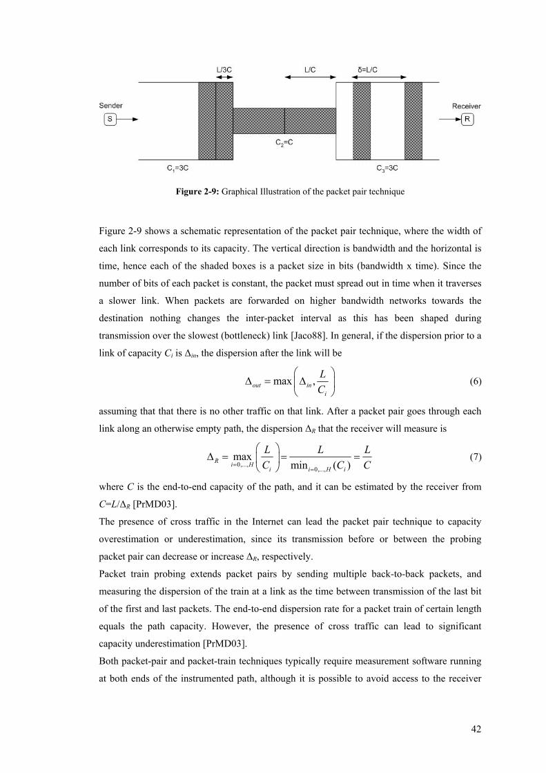
42

Figure 2-9: Graphical Illustration of the packet pair technique

Figure 2-9 shows a schematic representation of the packet pair technique, where the width of

each link corresponds to its capacity. The vertical direction is bandwidth and the horizontal is

time, hence each of the shaded boxes is a packet size in bits (bandwidth x time). Since the

number of bits of each packet is constant, the packet must spread out in time when it traverses

a slower link. When packets are forwarded on higher bandwidth networks towards the

destination nothing changes the inter-packet interval as this has been shaped during

transmission over the slowest (bottleneck) link [Jaco88]. In general, if the dispersion prior to a

link of capacity Ci is ∆in, the dispersion after the link will be

max ,out ini

LC

∆ = ∆

(6)

assuming that that there is no other traffic on that link. After a packet pair goes through each

link along an otherwise empty path, the dispersion ∆R that the receiver will measure is

0,...,

0,...,

maxmin ( )R i H

i i H i

L L LC C C=

=

∆ = = =

(7)

where C is the end-to-end capacity of the path, and it can be estimated by the receiver from

C=L/∆R [PrMD03].

The presence of cross traffic in the Internet can lead the packet pair technique to capacity

overestimation or underestimation, since its transmission before or between the probing

packet pair can decrease or increase ∆R, respectively.

Packet train probing extends packet pairs by sending multiple back-to-back packets, and

measuring the dispersion of the train at a link as the time between transmission of the last bit

of the first and last packets. The end-to-end dispersion rate for a packet train of certain length

equals the path capacity. However, the presence of cross traffic can lead to significant

capacity underestimation [PrMD03].

Both packet-pair and packet-train techniques typically require measurement software running

at both ends of the instrumented path, although it is possible to avoid access to the receiver

43

(by e.g. using some echo mechanism) at the expense of the reverse path capacity affecting the

accuracy of the results.

More recently, other methodologies have evolved to measure end-to-end available bandwidth

such as the Self-Loading Periodic Streams (SLoPS) [JaDo02] and the Trains of Packet Pairs

(ToPP) [MeBG00, MeBG02]. SLoPS send a stream of equal-sized packets from a source to a

receiver at a certain rate, and monitor the one-way delay variations of the probing traffic. If

the one-way delays increase then the stream rate is greater than the available bandwidth of the

path. The sender tries to bring the stream rate close to the available bandwidth by following an

iterative algorithm similar to binary search. ToPP send many packet-pairs at gradually

increasing rates from the source to the receiver at an initial dispersion, and then measures the

difference between the offered rate at the sender and receiver, respectively. The main

assumption (analogous to SLoPS) is that if the packet pair rate exceeds the end-to-end

available bandwidth, then the measured rate at the receiver will be less than the measured rate

at the sender.

There is a wide variety of mainly open source but also commercial tools for implementing the

different bandwidth estimation metrics, including per-hop and end-to-end capacity, available

bandwidth, TCP throughput and BTC estimation [Caid].

Recent studies have also examined the dependence of the different bandwidth estimation

algorithms with the end-host performance and examined cases where the measurement mostly

reflects the system throughput rather than the network bandwidth. System resources that affect

network bandwidth estimation include the resolution of the system timer, the time to perform

a system call, the interrupt delay (coalescing) enabled by some NICs, and the system I/O and

memory bandwidth. These studies suggest that VPS probing algorithms cannot accurately

measure capacity in high-speed (higher than OC-3 – 155 Mb/s) networks, whereas the

requirement for accurate packet dispersion measurement is the incoming packet dispersion to

be greater than the time for executing four system calls, two for getting the arrival time of

each packet and two for reading each packet. Packet train based algorithms are less sensitive

to the resolution of system timer and can work better on high-speed network environments,

since they measure the arrival time for a fixed but adjustable number of MTUs instead of

individual packets. In order to measure available bandwidth, the hosts involved need to be

able to handle data transfers higher than the available bandwidth, otherwise they will only be

able to measure the maximum throughput of the slower end-host [JiTi03].

44

2.3 Passive Measurements and Network Operations An alternative type of measurement methodology is to make passive measurements, in which

existing network traffic is recorded and analyzed. Passive techniques can completely eliminate

both additional traffic load and “Heisenberg” effects, in which the additional traffic perturbs

the network and biases the resulting analysis [Paxs96].

Passive measurements are deployed at a single observation point in the network and monitor

the operational traffic. Usually, the actual conclusive measurement is an offline activity of

passive measurement systems that either correlate data from multiple observation points in

order to implement even simple service-oriented performance metrics, or they post-process

monitoring data to draw aggregate measurement results regarding the operational state of the

network and the traffic carried through it. Because passive techniques observe the actual

traffic passing through a link, their results can be used as a direct or indirect input to network

operations and engineering processes.

Decomposition of passive measurements to further sub-categories can be made using a variety

of criteria such as the observation point they are employed on (e.g. router vs. probe vs.

terminal), the type of monitoring data they collect, and the level of hardware and/or software

support they require. In the following sections, the decomposition to different streams of

passive measurement systems is mainly based on the monitoring granularity they operate,

moving from observing aggregate per-link (interface) counters and statistics, to fine-grained

traffic flow and per-packet data.

In contrast to most active measurements that exploit common network and protocol

mechanisms and try to be otherwise transparent to network nodes, a characteristic shared

among all passive measurement systems is that they either require infrastructural support from

network nodes themselves, or they employ dedicated hardware-assisted configurations in

order to satisfy the tremendous processing and storage requirements imposed by the

untargeted operations of traffic monitoring, data storage, analysis and archiving of the

operational network traffic. Therefore, passive measurements is an area mostly governed by

the standardisation and deployment of specific systems whose primary design policy is not to

negatively impact the core forwarding operation of the network. Of particular importance is

also the transfer of monitoring data (usually over the network itself) for further, usually

centralised processing and analysis.

From a network operations and engineering perspective, passive measurements can be used

for long-term network planning and dimensioning but at the same time, and in conjunction

with other router data, they can be exploited for short-term traffic shaping and engineering

decisions. However, as it will be discussed later in this document, the main challenge

45

associated with passive measurements and network operations is the amount of data that needs

to be examined before any conclusive measurement can be conducted, and the consequential

difficulty of deploying feedback mechanisms to communicate network and/or traffic status

information in real-time. Complementary mechanisms to reduce the measurement data

without negatively impacting the correctness of the associated measurement, and hence

improve the scalability and performance of future real-time measurement and operations are

currently studied within this research area.

2.3.1 Simple Network Management Protocol (SNMP)

Although in the OSI world there is a distinction between element management20 and network

management21, in the IP world, network management has primarily been dealing with network

devices, that is, equipment whose sole purpose is to make the network operate properly

[Mart00]. Consequently, the Simple Network Management Protocol (SNMP) has been

designed to support the detail of network element management and to facilitate a systematic

way of querying the status of network elements to report on their operational status. The

element polling approach can indicate whether or not each network element is operating

within the configured operational parameters, and alert the network operator when there are

local anomalies to this condition [Hust00].

In May 1990, the first version of SNMP [CaFS90] together with a companion document

[RoMc90] on management information were published for monitoring and managing a

computer network. The wide implementation of the overall framework in commercial

products made SNMP the de facto standard for network management. The main entities of the

SNMP model are the managed nodes and the management stations (managers). A managed

node can be any (network) device (e.g. hosts, routers, printers) capable of communicating

status information to the outside world by running an SNMP agent process. Management

stations can be general-purpose computers running special management software which

communicate with the agents over a network, issuing commands and getting responses

[Tane96]. Agents run on devices that do not necessarily have the spare processing capacity for

accommodating management tasks, and henceforth all the intelligence is in the management

stations, trying to keep the impact of the agents minimal. Interoperability between

management stations and agents within multi-vendor computer networks is achieved by

standardising the exact information each kind of agent has to maintain and the format it has to

supply it in. Using the SNMP protocol, the manager communicates with the agents to access

(read and/or write) the agent Management Information Base (MIB), which is a collection of

20 Management of individual pieces of equipment 21 Management of an entire network abstracted as an entity on its own

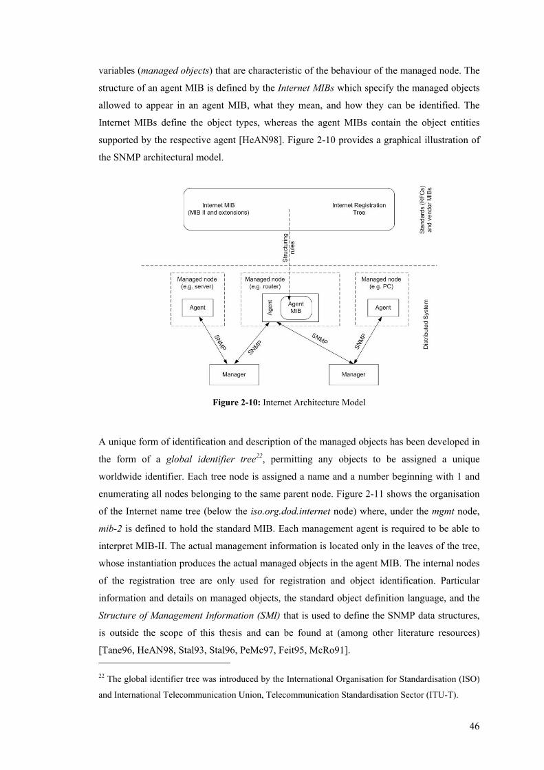
46

variables (managed objects) that are characteristic of the behaviour of the managed node. The

structure of an agent MIB is defined by the Internet MIBs which specify the managed objects

allowed to appear in an agent MIB, what they mean, and how they can be identified. The

Internet MIBs define the object types, whereas the agent MIBs contain the object entities

supported by the respective agent [HeAN98]. Figure 2-10 provides a graphical illustration of

the SNMP architectural model.

Figure 2-10: Internet Architecture Model

A unique form of identification and description of the managed objects has been developed in

the form of a global identifier tree22, permitting any objects to be assigned a unique

worldwide identifier. Each tree node is assigned a name and a number beginning with 1 and

enumerating all nodes belonging to the same parent node. Figure 2-11 shows the organisation

of the Internet name tree (below the iso.org.dod.internet node) where, under the mgmt node,

mib-2 is defined to hold the standard MIB. Each management agent is required to be able to

interpret MIB-II. The actual management information is located only in the leaves of the tree,

whose instantiation produces the actual managed objects in the agent MIB. The internal nodes

of the registration tree are only used for registration and object identification. Particular

information and details on managed objects, the standard object definition language, and the

Structure of Management Information (SMI) that is used to define the SNMP data structures,

is outside the scope of this thesis and can be found at (among other literature resources)

[Tane96, HeAN98, Stal93, Stal96, PeMc97, Feit95, McRo91]. 22 The global identifier tree was introduced by the International Organisation for Standardisation (ISO)

and International Telecommunication Union, Telecommunication Standardisation Sector (ITU-T).

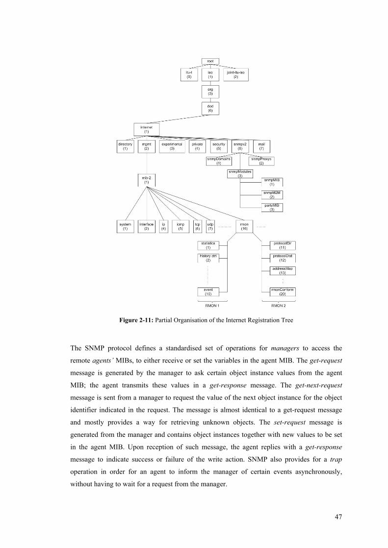
47

Figure 2-11: Partial Organisation of the Internet Registration Tree

The SNMP protocol defines a standardised set of operations for managers to access the

remote agents’ MIBs, to either receive or set the variables in the agent MIB. The get-request

message is generated by the manager to ask certain object instance values from the agent

MIB; the agent transmits these values in a get-response message. The get-next-request

message is sent from a manager to request the value of the next object instance for the object

identifier indicated in the request. The message is almost identical to a get-request message

and mostly provides a way for retrieving unknown objects. The set-request message is

generated from the manager and contains object instances together with new values to be set

in the agent MIB. Upon reception of such message, the agent replies with a get-response

message to indicate success or failure of the write action. SNMP also provides for a trap

operation in order for an agent to inform the manager of certain events asynchronously,

without having to wait for a request from the manager.

48

The second version of the SNMP protocol (SNMPv2) [CaMR93] extends the protocol

operations to include the get-bulk-request message with which the manager can ask for the

entire table of agent’s variables, minimising the number protocol exchanges required to

retrieve a large amount of management information. SNMPv2 also defines the inform-request

message for manager-to-manager communication, and the Snmpv2-trap message to provide

better support for asynchronous events.

SNMPv2 aimed at improving some of the limitations imposed by the first version of the

protocol, including the weak security concept, the inefficient transmission of large amounts of

management data, the manager-centric polling scheme, and the use of the connectionless UDP

transport for the encapsulation of SNMP messages. However, recent efforts to integrate a new

security concept and other improvements into Internet Management have led to the definition

and standardisation of SNMPv3 through a collection of IETF standards documents

[HaPW02]. A modular management framework under which agents will be able to operate

several different security models, encryption mechanisms, and SNMP message formats

simultaneously, was among the primary goals for the latest SNMP version, together with a

less static allocation of management functionality [HeAN98]. SNMPv3 aims at defining an

architecture that will allow for longevity of SNMP, extensibility, minimal implementations,

and at the same time will support more complex features required in large networks [ScPr04].

2.3.1.1 Standardised SNMP-based Network Monitoring: RMON and RMON2

The Remote MONitoring (RMON) MIB is a standardised set of managed objects to provide

for LAN measurement logging within the SNMP model of operation. In contrast to other

MIBs that are mainly concerned either with the operational status of the managed node and its

services (e.g. Host Resources MIB, Mail Monitoring MIB) or with its networking status (e.g.

Interfaces, Protocols groups of MIB-II), RMON is particularly oriented towards LAN

supervision (also below the IP layer) and represents the abstraction of a network probe.

RMON places higher demands on the supporting agents than those of a standard MIB II,

because it also defines the results of statistical calculations as managed objects. Hence, remote

monitoring devices can often be standalone boxes that devote a significant amount of internal

resources for managing a network, and the objects defined within the RMON MIB are

intended as an interface between a RMON agent and a RMON management application. The

offline operation, proactive monitoring, and problem detection and reporting are among the

primary goals of remote network management. The RMON MIB allows a probe to perform

diagnostics and collect performance, fault and configuration information without continuous

communication with manager being necessary. The monitor can log and store performance

information which can then be played back by the management station in order to get

49

historical knowledge and perform further empirical diagnosis into the cause of a problem

[Wald00].

As it can be seen in Figure 2-11, the RMON MIB occupies sub-tree 16 below the structural

node mib-2 in the Internet registration tree, and consists of ten MIB groups. Overall, it

comprises more than 200 managed objects, but all groups remain optional, hence RMON-

conformant products do not have to support all groups [HeAN98]. However, if a remote

monitoring device supports a particular group, it must implement all objects in that group. The

RMON objects are arranged into the ethernet statistics, history control, ethernet history,

alarm, host, hostTopN, matrix, filter, packet capture, and event groups. The ethernet statistics

group contains management information for each monitored ethernet interface (and therefore

for multiple segments simultaneously) on the device, including number of packets, bytes,

broadcasts, multicasts, information on lost packets, collisions, CRC and MTU-related errors.

The history control group controls the periodic statistical sampling of data from different

types of networks, including monitoring frequency and measurement intervals for individual

interfaces, and the ethernet history group records and stores periodic statistical samples from

ethernet segments. The alarm group compares absolute and relative changes in measurement

values from managed objects to previously defined thresholds, and generates events (alarms)

through the SNMP trap mechanism if the thresholds are exceeded. The host group contains

statistical information about each host generating traffic in the network segment by

monitoring the MAC addresses in the packets. The group consists of several tables that

contain the hosts to be monitored, the measurement periods, and the measurement data

(packets/bytes sent and received, broadcasts, errors). The hostTopN group depends on the host

group and categorises monitored hosts on a descending list based on one of their measured

values. The matrix group maintains statistics for traffic exchanged between pairs of hosts

based on their MAC addresses, and can potentially create traffic matrices for the monitored

network segments. The filter group enables the definition of packet filters based on bit

patterns in packets (data filters), on packet status information (status filters) and on higher-

level conditional expressions (complex filters). Packet streams that satisfy certain filtering

criteria are classified as channels which in turn can have counters and events associated with

them. The packet capture group allows packets to be captured if they satisfy some filtering

criterion, specified by the filter group. Finally, the event group controls the definition and

generation of events that can trigger actions defined elsewhere in the MIB. It can create a log

entry in the probe or send a SNMP trap, thus enabling asynchronous operation and helping to

eliminate the need for periodic polling from the management station.

Although the RMON MIB contains certain objects specifically targeted at ethernet networks,

its design allows for generically managing any type of network, as well as other specific

50

network types (e.g. Token Ring), through the definition of similarly appropriate objects

[Wald00].

The RMON2-MIB was later developed to double the MIB groups below mib-2.16, by adding

an additional ten-group sub-tree. The main motivation for the RMON2 definition [Wald97]

was to supplement the analysis of RMON that was focused on the first two layers of the OSI

model, and extend it up to and including the application layer. This extended analysis overall

improves network monitoring since more information processing takes place on the RMON

agent (remote system), and the SNMP data transfer from the agent to the manager is reduced

[HeAN98]. The monitoring objects are organised into ten additional MIB groups under the

mib-2.rmon structural node. The protocolDir group provides a table of all the protocols the

agent is able to decode, together with information about their parameters and SNMP message

structures. The ProtocolDistribution group computes protocol-related statistics for packets on

each monitored interface to produce a taxonomy of byte-counts and relative occurrence for

protocols at each layer. The addressMap group provides mappings between MAC and

network addresses of hosts on the monitored network segments and supports the generation of

network topology maps. The networkLayerHost group collects statistics for traffic sent and

received by each monitored device (network address), and the networkLayerMatrix group

provides information on the amount of traffic exchanged between pairs of monitored devices.

Similarly, applicationLayerHost and applicationLayerMatrix groups show the amount of

traffic for each protocol sent and received by the devices on the monitored segments and

between pairs of devices, respectively. The userHistory group allows for periodic sampling of

application-specific data and user-configured counters, to assist either with proactive or

reactive monitoring. The probeConfiguration and rmonConformance groups are used to

configure the RMON device and manage interoperability of different implementations.

RMON and RMON2 are considerably more advanced than the rest of the SNMP MIBs, since

they carry network monitoring data pre-processing and statistical computations at the agent,

and can hence minimise the data exchange between agents and management stations. RMON

agents can also be concurrently communicating monitoring data and statistics to multiple

managers responsible for different units and/or functions within the network.

Like any other MIB definition, the RMON1 and RMON2 standards define the way in which a

manager can retrieve information from probes, and which pieces of information are available.

However, RMON1/2 advantages come at the expense of complicated table management and

often the need for complex agents to be implemented in dedicated devices, hence a number of

network components only partially integrate RMON agents (often only the first four groups of

the RMON1 MIB) [HeAN98]. As it has been published by Cisco Systems23 in a Network

23 http://www.cisco.com/

51

Management System (NMS) white paper, supporting four RMON groups (e.g. statistics,

history, alarms and events) requires approximately 450 K code space whereas the dynamic

memory requirement for RMON varies, depending on the runtime configuration. Exemplary,

the statistics group would require 140 bytes of DRAM space per switched Ethernet or

FastEthernet port, and the alarm and event groups would require 2.6 K of memory per alarm

and its corresponding event entries [NMS]. RMON agents also need sophisticated SNMP

managers to configure them properly and take advantage of their capabilities to analyse the

collected network statistics. Due to MIBs’ complexity, RMON agents are almost uniquely

deployed by advanced network managers in only a number of large institutions [DeSu00].

Implementing the level of intelligence required by this new generation of MIBs requires more

than conventional MIB tools and compilers, and some research has focused on building a

nested-agent architecture, where a master agent facilitates dynamic loading of sub-agents to

carry group-specific tasks without affecting the performance of the master agent24.

OPNET Technologies Inc.25 have incorporated RMON probes among other passive and active

measurement techniques in their commercial monitoring packages which are targeted at being

deployed mainly in large enterprise and service provider networks. These bundles aim at

providing insight on the operational status of network devices, protocols, applications and

network services, and at facilitating among others network design, capacity planning

application deployment and service level agreement management [CPMT]. Infosim GmbH &

Co. KG26 provide the StableNet® PME network monitoring platform which is built upon open

standards, and it consists of single or clustered servers and distributed agents. StableNet aims

at providing for reliable and scalable monitoring of large IT systems and meet high

availability demands27. Among a large variety of measurement tools and methods for

topology, SLA reporting and application performance, StableNet® PME implements the

RMON MIB mainly to provide for ethernet packet-size analysis28. Triticom™ have designed a

number of software-based network monitoring tools, including the RMONster3229 which is a

distributed LAN monitoring package implementing the RMON1/2 MIB groups. The tool can

be installed on commodity hardware computers running a Microsoft® 32-bit Operating

System which will then function as a full-time RMON agent for the Ethernet or Token Ring

network it is attached to.

24 http://www.snmp.com/products/emanate.html 25 http://www.opnet.com/ 26 http://www.infosim.net/ 27 http://www.infosim.net/stablenet/stablenetPME/ 28 http://www.infosim.net/stablenet/stablenetPME/measurements/ 29 http://www.triticom.com/triticom/RMON32/

52

2.3.1.2 Open-source, SNMP-based Monitoring Tools

More popular, open-source SNMP-based network monitoring tools which have been widely

deployed for research as well as for production networks, are mainly used to query SNMP

data contained in groups directly under the MIB-II structural node, (such as e.g. the interface,

system, ip, tcp group), correlate it and visualise it. The Multi Router Traffic Grapher (MRTG)

is a tool written by Tobias Oetiker in 1995 to monitor the status of a 64 kb/s Internet link. The

tool’s first version was a Perl script using external utilities to execute SNMP queries and to

create visualisations of the results within HTML pages. The quick and wide spread of MRTG

as soon as it was published on the Internet, showed the great interest of people in network

monitoring tools, and also led to significant improvisation of the tool to provide for scalability

and portability, since the original design could only accommodate a small number of

monitored links. The second version of MRTG builds a skeleton configuration file for each

monitored router by reading its interface via SNMP and one of the tool’s key features is the

lossy data storage which stores traffic data with a decreasing resolution into the past. MRTG-2

can monitor any chosen SNMP variable for up to approximately 600 router ports in a 5-

minute interval. The unique feature of integrating data collection, storage, consolidation, and

visualisation in a single package gave MRTG an increasing popularity within the Internet

community30 [Oeti98]. MRTG was also influential in the development of other SNMP-based

monitoring tools that mainly aimed at improving its scalability and performance properties.

The Real Traffic Graber (RTG) was one such deployment which collected time-series SNMP

data from a large number of targets faster and more efficiently. RTG randomised the target

router list before polling, and hence minimised the performance overhead of each polled

SNMP agent having to deliver all its monitored objects at once. Individual object identifiers of

the devices are polled at random, and the polling thread does not block waiting for the device

query to timeout. Additionally, RTG tries to minimise the amount of data stored and

processed by using a database schema where a table per unique device and object is created to

only hold the interface identifiers, a polling timestamp, and a byte-count columns. RTG has

been reported to outperform its predecessor both by the number of monitored systems it is

able to cope with, as well as by minimising CPU utilisation [Beve02].

30 The third version of MRTG has been designed to be a generalised toolkit for applications that

monitor large numbers of diverse time-series data sources, rather than an application only for network

monitoring [Oeti98].

53

2.3.2 Flow Measurements

Early studies on measuring and characterising Internet traffic dynamics focused exclusively

on “packets” as being the fundamental unit of Internet traffic, and mainly concentrated on the

statistical nature of packet arrivals to uncover characteristics of traffic at the packet-level.

Although one can argue that packet-level measurements still maintain much of their

popularity within the relevant research community, the notion of the flow was introduced to

create an abstraction from packets, and to naturally link packet-level dynamics with

application-level dynamics, hence supporting special-service capabilities within the datagram

architecture of the Internet [Clar88]. IP flows are groups of packets that share common

characteristics among some of their protocol fields, mainly at the adjacent network and

transport layers of the networking stack. Such characteristics can among others be the IP

source and destination addresses, Type of Service (ToS) field, transport protocol, and

transport layer ports. A flow is a stream of packets comprising a portion of traffic subject to a

flow specification and delimited by a start and stop time. The start time of a flow is fixed for a

given flow, but the stop time may increase with the age of the flow [BrMR99]. Flow

definitions highly depend on the research context and therefore, different specifications have

been used to describe the type of service hosts need from the internetwork [Part92], or to

facilitate protocol-specific flow classification [RaCC04].

Within the context of (inter)network measurement research, the high flexibility and

parameterise-ability of flow specification and timeout values are largely influencing the

resulting flow statistics, and allow flow-based measurements to be exploited for a wide range

of network and traffic engineering tasks. These include network planning and performance

evaluation, routing optimisation, integration of networking technologies at different layers,

and attribution of network usage to users.

Early work on traffic flow profiling was influenced by the packet-train model of packet

arrivals which stated that if the spacing between two packets in a burst exceeds some inter-

train gap, they are said to belong to different trains [JaRo86]. The resulting parameterise-able

definition of flows identified four aspects in their specification, and explored how these

aspects interact with the flow timeout values [ClBP95]. Flow directionality specifies whether

flows should be defined as unidirectional or bi-directional and one versus two endpoint

aggregations distinguish between traffic with common network pairs and traffic aggregated at

either its source or its destination. The endpoint granularity specifies the flow aggregation

level, ranging from application to Internet backbone, and the protocol layer provides explicit

beginning and end of a flow by means of a transport or application level protocol.

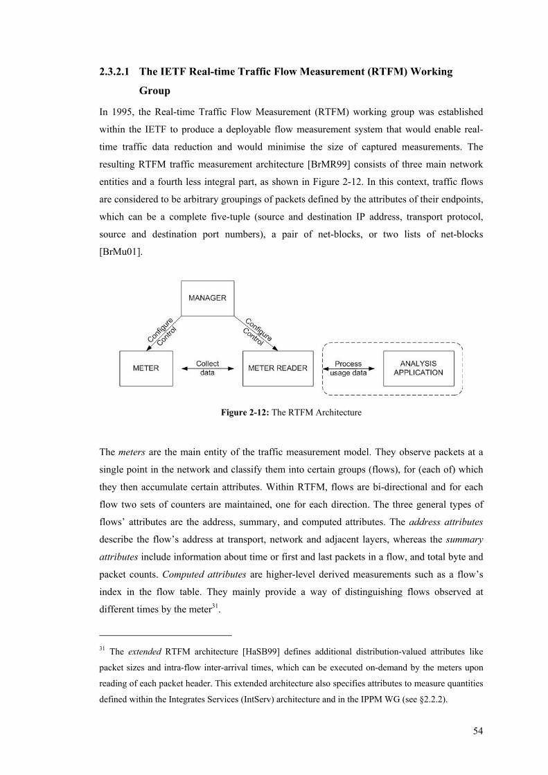
54

2.3.2.1 The IETF Real-time Traffic Flow Measurement (RTFM) Working

Group

In 1995, the Real-time Traffic Flow Measurement (RTFM) working group was established

within the IETF to produce a deployable flow measurement system that would enable real-

time traffic data reduction and would minimise the size of captured measurements. The

resulting RTFM traffic measurement architecture [BrMR99] consists of three main network

entities and a fourth less integral part, as shown in Figure 2-12. In this context, traffic flows

are considered to be arbitrary groupings of packets defined by the attributes of their endpoints,

which can be a complete five-tuple (source and destination IP address, transport protocol,

source and destination port numbers), a pair of net-blocks, or two lists of net-blocks

[BrMu01].

Figure 2-12: The RTFM Architecture

The meters are the main entity of the traffic measurement model. They observe packets at a

single point in the network and classify them into certain groups (flows), for (each of) which

they then accumulate certain attributes. Within RTFM, flows are bi-directional and for each

flow two sets of counters are maintained, one for each direction. The three general types of

flows’ attributes are the address, summary, and computed attributes. The address attributes

describe the flow’s address at transport, network and adjacent layers, whereas the summary

attributes include information about time or first and last packets in a flow, and total byte and

packet counts. Computed attributes are higher-level derived measurements such as a flow’s

index in the flow table. They mainly provide a way of distinguishing flows observed at

different times by the meter31.

31 The extended RTFM architecture [HaSB99] defines additional distribution-valued attributes like

packet sizes and intra-flow inter-arrival times, which can be executed on-demand by the meters upon

reading of each packet header. This extended architecture also specifies attributes to measure quantities

defined within the Integrates Services (IntServ) architecture and in the IPPM WG (see §2.2.2).

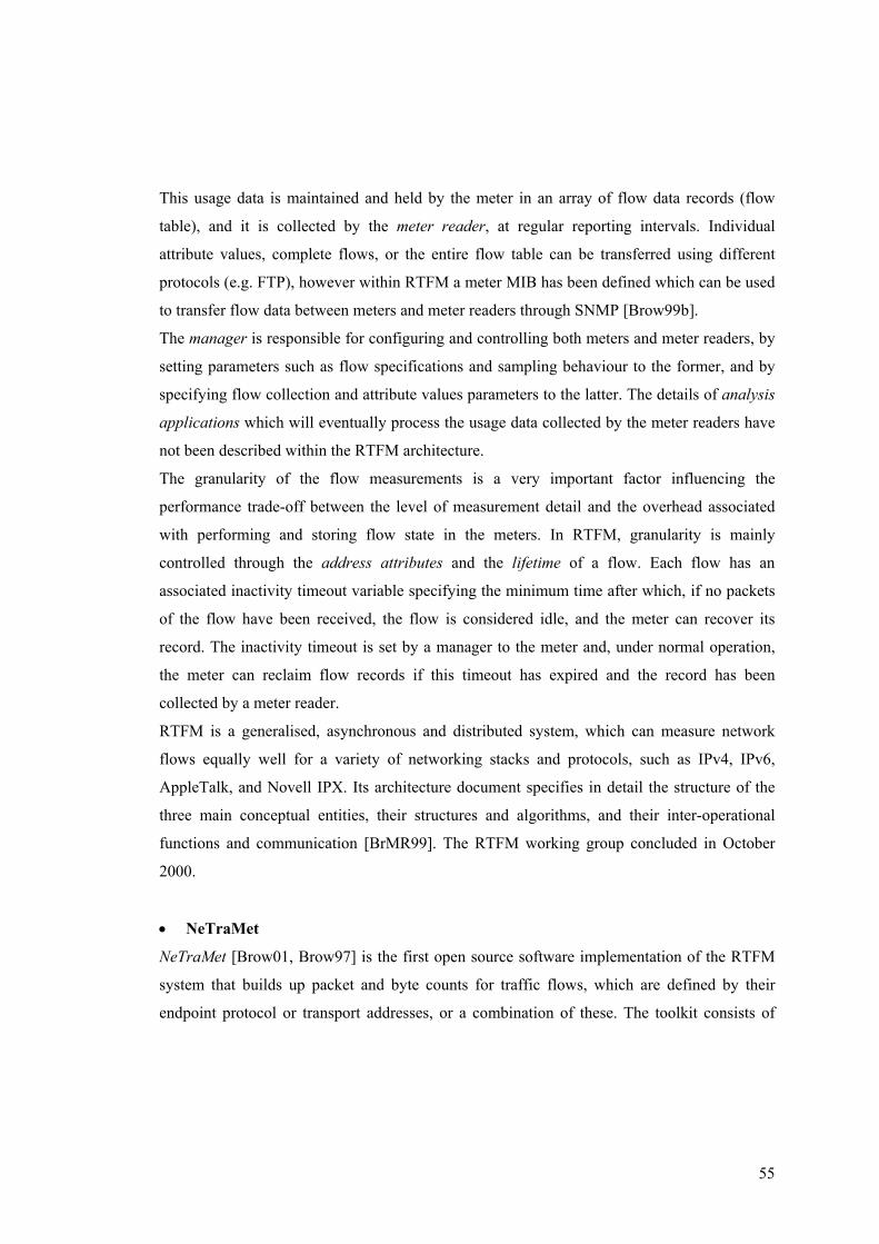
55

This usage data is maintained and held by the meter in an array of flow data records (flow

table), and it is collected by the meter reader, at regular reporting intervals. Individual

attribute values, complete flows, or the entire flow table can be transferred using different

protocols (e.g. FTP), however within RTFM a meter MIB has been defined which can be used

to transfer flow data between meters and meter readers through SNMP [Brow99b].

The manager is responsible for configuring and controlling both meters and meter readers, by

setting parameters such as flow specifications and sampling behaviour to the former, and by

specifying flow collection and attribute values parameters to the latter. The details of analysis

applications which will eventually process the usage data collected by the meter readers have

not been described within the RTFM architecture.

The granularity of the flow measurements is a very important factor influencing the

performance trade-off between the level of measurement detail and the overhead associated

with performing and storing flow state in the meters. In RTFM, granularity is mainly

controlled through the address attributes and the lifetime of a flow. Each flow has an

associated inactivity timeout variable specifying the minimum time after which, if no packets

of the flow have been received, the flow is considered idle, and the meter can recover its

record. The inactivity timeout is set by a manager to the meter and, under normal operation,

the meter can reclaim flow records if this timeout has expired and the record has been

collected by a meter reader.

RTFM is a generalised, asynchronous and distributed system, which can measure network

flows equally well for a variety of networking stacks and protocols, such as IPv4, IPv6,

AppleTalk, and Novell IPX. Its architecture document specifies in detail the structure of the

three main conceptual entities, their structures and algorithms, and their inter-operational

functions and communication [BrMR99]. The RTFM working group concluded in October

2000.

• NeTraMet

NeTraMet [Brow01, Brow97] is the first open source software implementation of the RTFM

system that builds up packet and byte counts for traffic flows, which are defined by their

endpoint protocol or transport addresses, or a combination of these. The toolkit consists of

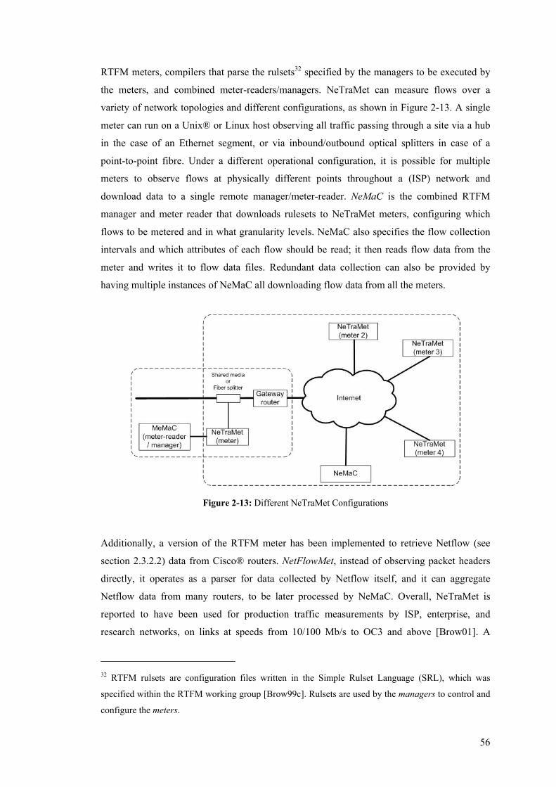
56

RTFM meters, compilers that parse the rulsets32 specified by the managers to be executed by

the meters, and combined meter-readers/managers. NeTraMet can measure flows over a

variety of network topologies and different configurations, as shown in Figure 2-13. A single

meter can run on a Unix® or Linux host observing all traffic passing through a site via a hub

in the case of an Ethernet segment, or via inbound/outbound optical splitters in case of a

point-to-point fibre. Under a different operational configuration, it is possible for multiple

meters to observe flows at physically different points throughout a (ISP) network and

download data to a single remote manager/meter-reader. NeMaC is the combined RTFM

manager and meter reader that downloads rulesets to NeTraMet meters, configuring which

flows to be metered and in what granularity levels. NeMaC also specifies the flow collection

intervals and which attributes of each flow should be read; it then reads flow data from the

meter and writes it to flow data files. Redundant data collection can also be provided by

having multiple instances of NeMaC all downloading flow data from all the meters.

Figure 2-13: Different NeTraMet Configurations

Additionally, a version of the RTFM meter has been implemented to retrieve Netflow (see

section 2.3.2.2) data from Cisco® routers. NetFlowMet, instead of observing packet headers

directly, it operates as a parser for data collected by Netflow itself, and it can aggregate

Netflow data from many routers, to be later processed by NeMaC. Overall, NeTraMet is

reported to have been used for production traffic measurements by ISP, enterprise, and

research networks, on links at speeds from 10/100 Mb/s to OC3 and above [Brow01]. A

32 RTFM rulsets are configuration files written in the Simple Rulset Language (SRL), which was

specified within the RTFM working group [Brow99c]. Rulsets are used by the managers to control and

configure the meters.

57

variant version of the software also exists that uses the CoralReef architecture (see section

2.3.3.4) to access packet headers collected by dedicated ATM measurement cards [DAG]. If

hardware vendors choose to implement the RTFM meter MIB in switches and routers, then

the RTFM system can avoid deploying software-based meters. Instead, they would then

become an integral part of the Internet switching infrastructure, substantially improving the

performance requirements, overhead, and widespread use of RTFM/NeTraMet.

The NeTraMet implementation has been further used by researchers to characterise Internet

flows based on their lifetime as well as on their byte volumes. These studies decomposed

measured traffic into three granularity categories: streams were defined to be individual IP

sessions between ports on pairs of hosts, flows are sets of packets travelling between two net-

blocks (hosts or networks) in either direction, and torrents describe the overall traffic

aggregate on a given link [BrMu01]. It was suggested that streams can be classified not only

by their size33, but also by their lifetime into dragonflies lasting up to two seconds, short

lasting up to fifteen minutes, and tortoises lasting more than fifteen minutes. Measurements

over specific Internet paths revealed that although about 1.5% of streams were long-running,

up to 50% of all bytes were accounted to these tortoises [BrCl02].

Recent studies also focused on defining dynamic flow timeout algorithms, arguing that a fixed

timeout identical for all flows which had been used in the past, was not optimal to satisfy the

high variability between different flow durations. NeTraMet uses packet inter-arrival times of

the streams comprising a flow to compute its inactivity time [BrMu01], whereas a different

study suggested an adaptive flow timeout strategy based on the flow’s throughput during its

initial period, in order to preserve long-lived flows and at the same time minimise flow-

holding times [RyCB01].

2.3.2.2 Cisco IOS® Netflow

Netflow34 is a flow measurement technology to collect data as it enters specific routers or

switches interfaces, and analyse it to provide for a number of network operations tasks. Being

an integral part of Cisco IOS software, Netflow has evolved to the de facto standard for flow

monitoring, since it enables Cisco product-based35 networks to perform traffic flow analysis

without the need of purchasing and configuring custom probes. Service providers can use

Netflow to measure traffic flows on their Points-Of-Presence (POP), peering or transit points,

33 Early analysis on TCP behaviour had classified streams into network elephants (high-volume) and

network mice (small streams). Their fundamental difference is that elephants extend past TCP’s slow

start phase and are hence subject to feedback-based congestion control algorithms [JoRF99]. 34 http://www.cisco.com/warp/public/732/Tech/nmp/netflow/ 35 Netflow is also implemented by other vendors [MoQu04]

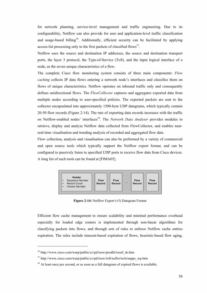
58

for network planning, service-level management and traffic engineering. Due to its

configurability, Netflow can also provide for user and application-level traffic classification

and usage-based billing36. Additionally, efficient security can be facilitated by applying

access-list processing only to the first packets of classified flows37.

Netflow uses the source and destination IP addresses, the source and destination transport

ports, the layer 3 protocol, the Type-of-Service (ToS), and the input logical interface of a

node, as the seven unique characteristics of a flow.

The complete Cisco flow monitoring system consists of three main components: Flow

caching collects IP data flows entering a network node’s interfaces and classifies them on

flows of unique characteristics. Netflow operates on inbound traffic only and consequently

defines unidirectional flows. The FlowCollector captures and aggregates exported data from

multiple nodes according to user-specified policies. The exported packets are sent to the

collector encapsulated into approximately 1500-byte UDP datagrams, which typically contain

20-50 flow records (Figure 2-14). The rate of exporting data records increases with the traffic

on Netflow-enabled nodes’ interfaces38. The Network Data Analyser provides modules to

retrieve, display and analyse Netflow data collected from FlowCollector, and enables near-

real-time visualisation and trending analysis of recorded and aggregated flow data.

Flow collection, analysis and visualisation can also be performed by a variety of commercial

and open source tools which typically support the Netflow export format, and can be

configured to passively listen to specified UDP ports to receive flow data from Cisco devices.

A long list of such tools can be found at [FlMA05].

Figure 2-14: Netflow Export (v5) Datagram Format

Efficient flow cache management to ensure scalability and minimal performance overhead

especially for loaded edge routers is implemented through non-linear algorithms for

classifying packets into flows, and through sets of rules to enforce Netflow cache entries

expiration. The rules include timeout-based expiration of flows, heuristic-based flow aging,

36 http://www.cisco.com/warp/public/cc/pd/iosw/prodlit/iosnf_ds.htm 37 http://www.cisco.com/warp/public/cc/pd/iosw/ioft/neflct/tech/napps_wp.htm 38 At least once per second, or as soon as a full datagram of expired flows is available.

59

and observation of explicit transport mechanisms indicating flow termination (e.g. TCP FIN

or RST flags). Aggregation caches can also be enabled to maintain grouped flows based on

different fields’ combinations of individual flows, providing for router-based aggregation that

improves cache management and at the same time reduces the export data volume. The main

flow aggregation schemes are based on autonomous system, source and destination prefix and

protocol port. Additional schemes include the ToS byte as a field39.

The Netflow cache size is configurable, yet its default values vary for different Cisco

platforms with respect to their available Dynamic Random Access Memory (DRAM).

A number of different versions of the Netflow export data format have been defined as a result

of continuous enhancements on the information the flow export datagrams carry. The main

fields of individual flow records include the flow’s packet and byte counts, the start and stop

times for the flow, and a cumulative indication of the flow’s TCP flags, in addition to the

seven unique characteristics reported earlier that Netflow uses to define a flow.

Enabling Netflow on Cisco network nodes results in an anticipated performance overhead in

terms of CPU utilisation and system resources, which increases with the number of flows

monitored and maintained in the flow cache, but not with the individual Netflow features

enabled (e.g. aggregation). The overhead is particularly noticeable on nodes that normally

perform most forwarding decisions directly in hardware, where a software-based Netflow

version can bypass the hardware forwarding mechanism40.

The Sampled Netflow feature was developed to scale the flow measurement operation to high

forwarding rates, allowing a node to sample only one out of N forwarded packets to be

accounted for in the Netflow flow cache.

Recent studies focused on defining efficient sampling algorithms to identify and measure only

large flows that account for the highest percentage of the overall Internet traffic. The sample

and hold algorithm samples a packet with a probability depending on the byte-size of a flow,

and for each sampled packet, all subsequent packets belonging on the same flow are also

sampled. The multistage filters algorithm uses independent hash functions (stages) in parallel

to classify packets based on their flow characteristics, and increase a flow-related counter with

the size of each packet. Flows whose counter (representing their size) exceeds a specified

threshold at all stages are added to the flow memory [EsVa02]. Such algorithms aim at

minimising both the processing and flow collection overheads, by only keeping flow state of a

few large flows using a small amount of fast memory in network nodes.

Dynamic adaptation of the sampling rate has also been recently introduced, specifically to

improve Netflow’s robustness, by setting a maximum sampling rate and then dynamically

39 http://www.cisco.com/univercd/cc/td/doc/cisintwk/intsolns/netflsol/nfwhite.htm 40 http://www.cisco.com/warp/public/cc/pd/iosw/prodlit/ntfo_wp.htm

60

decreasing it until it is low enough for the flow records to fit into a specified amount of

memory [EsKM04].

2.3.2.3 The Internet Protocol Flow Information eXport (IPFIX) Working

Group

The IPFIX Working Group has been established in October 2001 within the IETF, to provide

Internet standards on the way network devices export flow information to external systems for

measurement post-processing and analysis [IPFIX]. Standardising a data model to represent

flow information and a transport protocol to transfer this information between flow exporters

and collection stations, aims at facilitating the deployment of inter-operable, multi-vendor

systems to enable research, measurement, network management, accounting and billing

services. The IPFIX requirements document which has been submitted for publication as an

informational RFC, identifies a list of attributes that a compliant flow exporter must be able to

report, and highlights certain security and scalability characteristics for the flow export

process. The flow attributes include the IP version, the source and destination IP addresses,

the IP protocol type, the source and destination transport ports, the flow’s total packet counter

(also counting packet fragments), the flow’s total byte counter (including IP header and

payload); timestamps for the first and last packets in the flow, a unique identifier of the

observation point and of the exporting process, and the sampling configuration used for the

measurement. Also, depending on the IP version of the flow, the ToS octet (for IPv4 flows),

or the traffic class octet and Flow Label field (for IPv6 flows) is included. If Multi-Protocol

Label Switching (MPLS) is supported, the exporter must also report the top MPLS label or the

corresponding Forwarding Equivalence Class (FEC) [QuZC04]. Additional attributes have

also been specified that an exporter can optionally support, such as TCP header flags, IP TTL

field and Boarder Gateway Protocol (BGP) Autonomous System (AS) numbers. This list of

attributes is by no means exhaustive, and hence implementations of the flow information

export model should be extensible to accommodate for future compulsory and optional

attributes to be added. Moreover, the flow records should be transferred over a congestion

aware protocol, so as not to overwhelm the links between the exporters and the collection

stations, and also to exhibit certain reliability characteristics indicating loss of flow records

during the transfer process.

The IPFIX WG examined a number of candidate protocols that could potentially form the

basis of a standardised flow export protocol, and evaluated them against the major IPFIX

requirements. Individual characteristics that were assessed for each candidate protocol

included the reliability and security properties of the metering process, the degree of

extensibility of the protocol’s data model, the sampling support, the operational adaptation to

overload conditions, and the time synchronisation and flow expiration capabilities. The

61

evaluation team concluded that Netflow Version 941 format for exporting performance

information from network nodes would best serve the goals of the IPFIX charter [Lein04].

This latest version of Netflow technology’s (see section 2.3.2.2) flow-record format is mainly

distinguished from its predecessors by being template-based and hence offering the necessary

support for adaptation, inter-operability, and future enhancements. Each Netflow V9 exported

packet can contain normal flow-records, but also template records to define the format and

processing requirements of subsequent data (flow records) on-demand42.

The reader should note that, at the time of writing, the work within the IPFIX working group

is still in the process of being standardised by the Internet community.

2.3.3 Packet Monitoring

Capturing individual packets that traverse a network link has been a fundamental and arguably

the most popular passive measurement technique, extensively used in the research community

to characterise numerous properties of operational network traffic (e.g. [LeTW93, ApCT96,

ClMT98, FrDL01]), and to assess link utilisation and traffic demands (e.g. [FeGL01]), mainly

over backbone links and topologies. The technique is often referred to as monitoring, instead

of measurement, mainly because the majority of packet capturing infrastructures and tools

have been mainly used for retrospective, rather than on-the-fly analysis. Hence, the actual

measurement and characterisation is a post-processing and often offline task on the captured

traffic. Packet monitoring enables passive (non-intrusive) measurement of network and traffic

properties at the finest level of granularity, by tapping a link to receive a copy of each packet,

then collecting and analysing detailed IP packet traces on individual links in the network. By

treating packets as the basic monitored entity, the amount as well as the nature of the available

information can be used as input for a very long (if not endless) list of analytical studies.

These can include the investigation of packet inter-arrival times to characterise the nature of

network traffic (e.g. [LeTW93]), and the composition of different notions of flows to expose

the dominant presence of applications, protocols, packet sizes, flow size distributions, and

length of packet trains in the Internet (e.g. [ClMT98]). Measured properties of IP packet traces

can be used for modelling and simulating network behaviour (e.g. [ChLi98]), and for long or

short-term capacity planning and dimensioning by examining the adequacy of networks’

provisioning and load balancing. Additionally, correlation of multiple single-point

observations can be used to measure unidirectional traffic properties (e.g. [GrDM98,

FrDL01]) and to estimate network-wide traffic models (e.g. [GrRe02, Vard96]).

41 http://www.cisco.com/warp/public/732/Tech/nmp/netflow/netflow_ver9.shtml 42 http://www.cisco.com/en/US/tech/tk648/tk362/technologies_white_paper09186a00800a3db9.shtml

62

Packet monitoring is often considered as the predecessor and the basic building block for flow

measurements, which can in turn be viewed as an aggregate of packet-based traffic statistics

collection (see section 2.3.2). However, in this thesis, the classification of passive

measurements techniques is based on the level of collection detail, and the consequential

presentation granularity of each mechanism with respect to the network traffic properties that

can be measured and analysed. Under this viewpoint, router-based passive measurements

operate on a coarser granularity level, offering less flexibility in what traffic properties can be

inferred from the monitored data. SNMP/RMON-based techniques focus on network-element-

centric monitoring, only providing information for a set of managed objects that mainly

concern the interfaces of the nodes/hosts of a local sub-network (OSI layers 1 and 2). IP

packets are not the main monitored entity, and only cumulative information on the operation

of network interfaces is monitored. RMON2 extends this model to include managed objects

for the rest of the OSI layers, but is still providing only certain (standardised) aggregate, not

traffic-centric statistics for the monitored LAN segments (e.g. network-to-MAC address

mappings, protocol distribution per LAN segment). Flow measurement systems are clearly

more IP traffic-oriented, but due to their nature, the real-time packet-to-flow classification and

their strong coupling with router platforms, they only collect aggregate flow statistics. Hence

they do not offer intra-flow packet details nor do they concentrate directly on the interaction

between traffic belonging to different flows.

Packet monitoring systems are router-independent, and their operation does not influence the

performance of the network forwarding mechanisms. Consequently, they are not governed by

standardisation processes, and, by being able to capture and store detailed information on a

per-packet basis, they offer a great flexibility on what information they store and manipulate,

depending on the measurement analysis of interest.

The main infrastructural challenges of packet monitoring systems include the different ways

of getting access to the operational network traffic, and their hardware and/or software design

that will allow them to keep pace with the continuously increasing network link speeds. Also,

the amount of monitored data they need to store, process, and often ship though the network

to remote measurement analysis systems for offline processing can influence the overall

design of the infrastructure and the data reduction algorithms that need to be put in place to

minimise the related overhead. These main issues will be briefly described in the following

sections.

2.3.3.1 Shared Media Vs. Point-to-point Links

Depending on the type of network link a packet monitoring system operates, different setups

are used to receive a copy of each packet traversing that link. Packet monitors can be passive

terminals consisting of commodity hardware PC configurations equipped with monitoring

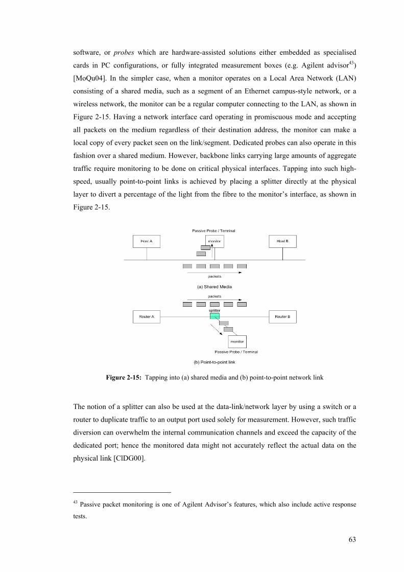
63

software, or probes which are hardware-assisted solutions either embedded as specialised

cards in PC configurations, or fully integrated measurement boxes (e.g. Agilent advisor43)

[MoQu04]. In the simpler case, when a monitor operates on a Local Area Network (LAN)

consisting of a shared media, such as a segment of an Ethernet campus-style network, or a

wireless network, the monitor can be a regular computer connecting to the LAN, as shown in

Figure 2-15. Having a network interface card operating in promiscuous mode and accepting

all packets on the medium regardless of their destination address, the monitor can make a

local copy of every packet seen on the link/segment. Dedicated probes can also operate in this

fashion over a shared medium. However, backbone links carrying large amounts of aggregate

traffic require monitoring to be done on critical physical interfaces. Tapping into such high-

speed, usually point-to-point links is achieved by placing a splitter directly at the physical

layer to divert a percentage of the light from the fibre to the monitor’s interface, as shown in

Figure 2-15.

Figure 2-15: Tapping into (a) shared media and (b) point-to-point network link

The notion of a splitter can also be used at the data-link/network layer by using a switch or a

router to duplicate traffic to an output port used solely for measurement. However, such traffic

diversion can overwhelm the internal communication channels and exceed the capacity of the

dedicated port; hence the monitored data might not accurately reflect the actual data on the

physical link [ClDG00].

43 Passive packet monitoring is one of Agilent Advisor’s features, which also include active response

tests.

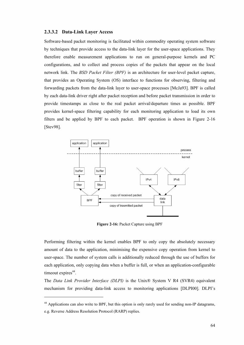
64

2.3.3.2 Data-Link Layer Access

Software-based packet monitoring is facilitated within commodity operating system software

by techniques that provide access to the data-link layer for the user-space applications. They

therefore enable measurement applications to run on general-purpose kernels and PC

configurations, and to collect and process copies of the packets that appear on the local

network link. The BSD Packet Filter (BPF) is an architecture for user-level packet capture,

that provides an Operating System (OS) interface to functions for observing, filtering and

forwarding packets from the data-link layer to user-space processes [McJa93]. BPF is called

by each data-link driver right after packet reception and before packet transmission in order to

provide timestamps as close to the real packet arrival/departure times as possible. BPF

provides kernel-space filtering capability for each monitoring application to load its own

filters and be applied by BPF to each packet. BPF operation is shown in Figure 2-16

[Stev98].

Figure 2-16: Packet Capture using BPF

Performing filtering within the kernel enables BPF to only copy the absolutely necessary

amount of data to the application, minimising the expensive copy operation from kernel to

user-space. The number of system calls is additionally reduced through the use of buffers for

each application, only copying data when a buffer is full, or when an application-configurable

timeout expires44.

The Data Link Provider Interface (DLPI) is the Unix® System V R4 (SVR4) equivalent

mechanism for providing data-link access to monitoring applications [DLPI00]. DLPI’s

44 Applications can also write to BPF, but this option is only rarely used for sending non-IP datagrams,

e.g. Reverse Address Resolution Protocol (RARP) replies.

65

operation closely resembles that of BPF, also supporting filtering within the kernel as well as

data and system call reduction through similar mechanisms. However, the BPF filter

implementation has been reported to outperform that of DLPI, being 3 to 20 times faster,

depending on the complexity of the filter [McJa93].

Under Linux®, access to the data-link layer is provided through a SOCK_PACKET type

socket. This feature does not support any filtering or buffering within the kernel, nor does it

support filtering by device. Hence, the overhead of copying all captured data from all devices

to user-space is obviously significantly larger than that of DLPI and BPF, in some cases by

orders of magnitude [Stev98, MoQu04].

The packet capture library, libpcap, provides an OS-independent interface to the different

underlying data-link access system facilities, such as the BPF, DLPI, and SOCK_PACKET.

The library’s performance depends on the underlying system-dependent mechanism used, and

maximum performance is limited by the packet copying and the context switching between

kernel and user-space. Libpcap is currently used by a lot of popular monitoring tools including

TCPdump45 and NeTraMet (section 2.3.2.1).

2.3.3.3 Hardware-Assisted Packet Capturing: DAG Cards (example)

Packet capturing over long timescales on high-capacity and backbone network links imposes

stringent demands at all levels of a monitoring process, on both system bandwidth and storage

capacity. The lack of support for specific measurement functionality (e.g. NIC timestamping)

on most commodity hardware, as well as the contradicting goals between modern OS design

and measurement processes, make purely software-based packet capturing inadequate to meet

the performance and accuracy requirements of monitoring high-speed critical interfaces

carrying large amounts of aggregate traffic. The way standard Network Interface Cards (NIC)

buffer and transfer data over the PCI bus, the OS-generated timestamps, the amount of kernel

level interrupts and processing, as well as the unreliability of network protocols below the

transport (TCP) level, are among the primary factors introducing overhead and inaccuracy in

software-based measurement on commodity PC configurations.

One of the most popular hardware-assisted passive monitoring solutions is the DAG cards,

initially developed within the University of Waikato, New Zealand, and now being produced

by Endace Measurement Systems46. DAG cards have been widely used in passive monitoring

research projects and infrastructures. Initial experiments in the DAG project focused on re-

programming ATM NICs to enable timestamping of ATM cells with an approximate accuracy

of one tenth of the cell time. This level of accuracy could not be achieved with commercial

45 http://www.tcpdump.org/ 46 http://www.endace.com/

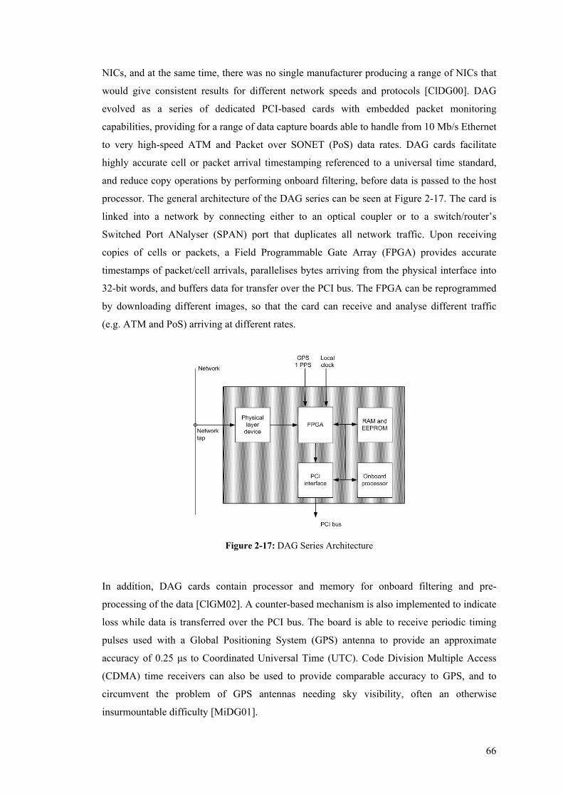
66

NICs, and at the same time, there was no single manufacturer producing a range of NICs that

would give consistent results for different network speeds and protocols [ClDG00]. DAG

evolved as a series of dedicated PCI-based cards with embedded packet monitoring

capabilities, providing for a range of data capture boards able to handle from 10 Mb/s Ethernet

to very high-speed ATM and Packet over SONET (PoS) data rates. DAG cards facilitate

highly accurate cell or packet arrival timestamping referenced to a universal time standard,

and reduce copy operations by performing onboard filtering, before data is passed to the host

processor. The general architecture of the DAG series can be seen at Figure 2-17. The card is

linked into a network by connecting either to an optical coupler or to a switch/router’s

Switched Port ANalyser (SPAN) port that duplicates all network traffic. Upon receiving

copies of cells or packets, a Field Programmable Gate Array (FPGA) provides accurate

timestamps of packet/cell arrivals, parallelises bytes arriving from the physical interface into

32-bit words, and buffers data for transfer over the PCI bus. The FPGA can be reprogrammed

by downloading different images, so that the card can receive and analyse different traffic

(e.g. ATM and PoS) arriving at different rates.

Figure 2-17: DAG Series Architecture

In addition, DAG cards contain processor and memory for onboard filtering and pre-

processing of the data [ClGM02]. A counter-based mechanism is also implemented to indicate

loss while data is transferred over the PCI bus. The board is able to receive periodic timing

pulses used with a Global Positioning System (GPS) antenna to provide an approximate

accuracy of 0.25 µs to Coordinated Universal Time (UTC). Code Division Multiple Access

(CDMA) time receivers can also be used to provide comparable accuracy to GPS, and to

circumvent the problem of GPS antennas needing sky visibility, often an otherwise

insurmountable difficulty [MiDG01].

67

Initially, the first series of DAG focused on packet monitoring over OC-3 and OC-12 links at

155 and 622 Mb/s, respectively. DAG-4 introduced an enhanced architecture for OC-48

monitoring at approximately 2.488 Gb/s, and DAG-6 is designed for packet capturing over

OC-192 links at 10 Gb/s47.

DAG monitors have been used to measure unidirectional properties over intercontinental

distances, by correlating packet traces captured by different monitors, each one attached to a

network of interest. Unidirectional delay, delay variation and packet loss have been measured

by matching different packets or cells at the ends of the measurements [ClGM02]. DAG-

based monitors have also been used to calibrate measurements done by the Skitter (section

2.2.3.2), TTM, Surveyor (sections 2.2.4.1 and 2.2.4.2) and AMP (section 2.2.5) projects.

2.3.3.4 Customised Hardware and Software Packet Monitoring Architectures

There exists a very long and continuously increasing list of commercial and open-source

software packet capturing/monitoring tools, yet their description here would be ineffectual

since it would not provide a deeper insight into measurement techniques and architectures,

and is indeed outside the scope of this thesis. The interested reader is referred to [SLAC] that

provides a comprehensive and regularly updated list of available network monitoring tools.

Such tools mainly build on top of common packet capture libraries and data-link access

technologies (see e.g. section 2.3.3.2), and mainly focus on the analysis and visualisation of

monitored packet data. Some of their features include the flexible specification of packet

filtering rules, the decomposition of traffic data down to individual hosts, protocols and

applications, and sometimes the troubleshooting or intruder detection and alarm generation

based on certain traffic load conditions [MoQu04]. TCPDump48 is definitely worth-

mentioning as an example, since it is the ancestor of many similar tools; it is based on libpcap

to read a configurable amount of bytes for each packet arriving at an interface and stores

captured data on disk. TCPdump uses a high-level syntax to implement sophisticated packet

filtering.

The remainder of this section provides a description of indicative research-driven customised

hardware (and software) monitoring platforms, mainly developed to passively capture data on

backbone and high-speed network links, and whose results were then used to characterise

Internet traffic behaviour and/or to provide for network operations and engineering tasks.

These architectures should mainly serve as examples of customised equipment that provide a

complete bundle for data link access, packet capture methodologies, and captured data

analysis techniques over high capacity network interfaces.

47 http://www.ist-scampi.org/events/workshop-2003/donnelly.pdf 48 http://www.tcpdump.org/

68

• OC*MON Systems

OC3MON [ApCT96] was among the first research-oriented, custom-built packet monitoring

platforms, developed just after mid-1990s by MCI49 and CAIDA within the context of

NSF’s50 very high speed Backbone Network Service (vBNS51) project. At the time, ATM

trunks at OC-3c had started being increasingly used for high-volume backbone links, and the

already widely deployed statistics gathering tools based on lower-capacity multi-access media

(e.g. FDDI and Ethernet) could not easily scale to higher speeds. Hence, the design of

OC3MON aimed at providing a flexible and relatively low-cost data collection and analysis

system to monitor these high-speed links, and to be easily extensible to operate on even higher

rates.

The monitor was built on an IBM-compatible PC and was equipped with two ATM interface

cards with an onboard processor that allowed custom firmware to be loaded to optimise the

system’s operation. The receive port of each ATM card connected to the monitor port of an

optical splitter, allowing OC3MON to capture traffic over an OC-3 link, in both directions.

OC3MON employed customised DOS-based software consisting of device drivers and a

TCP/IP stack, and higher-level software to perform real-time flow analysis. During the initial

design of the monitor, the otherwise less-advanced features of DOS provided better control

over the entire machine and its TCP/IP stack operation, lower interrupt latency than UNIX,

and more efficient card-to-host buffer transfers by not fragmenting the large blocks of

contiguous physical memory of the machine. However, a FreeBSD UNIX port of OC3MON

was soon developed and released, in response to community feedback.

The monitor supports raw cell trace capture, active flow reporting, and expired flow analysis,

as three different modes of data collection. When operating in the first mode, OC3MON

produces a timestamped raw cell trace of either every cell or the first cell of every AAL5

frame, without further analysing the captured data. In the other two modes, the monitor

collects statistics regarding active or expired flows using configurable flow definitions.

OC3MON has been used to report utilisation statistics and packet size distributions of

backbone trunks, as well as to derive flow profile information from captured packets and

produce parameterise-able flow statistics analysis.

A highly-cited Internet backbone measurements study based on traffic statistics collected by

OC3MON systems revealed some important properties for the nature of the Internet

[ClMT98]. Among others, it was stated that 60% of packets seen in MCI’s backbone are 44 49 http://www.mci.com/ 50 http://www.nsf.gov/ 51 http://www.vbns.net/

69

bytes or less, however, they constitute 7% of the byte volume; over half of the bytes are

carried in packets of size 1500 bytes or larger. TCP was reported to dominate the traffic mix,

contributing to approximately 95% of bytes, 90% of packets, and 80% of the flows on the

monitored links. Web traffic also dominated the monitored links, comprising up to 75% of the

bytes, 70% of the packets, and 75% of the flows, when client and server traffic are considered

together. Although this study has been conducted in 1998, it is widely believed (and

sometimes proven from recent measurement studies) that the broad nature of the Internet still

remains largely the same.

When MCI’s backbone transitioned from OC-3 to OC-12 rates, OC3MON naturally evolved

to the OC12MON, which used new OC12 ATM cards and generally maintained almost the

same specifications. The whole backbone OC monitoring project has been progressively

renamed to the Coral measurement architecture, which became the ancestor of the more

recent CoralReef suite (described below).

• Sprint Backbone IP Monitoring Project

The IP Monitoring (IPMON) project52 deployed a passive packet monitoring and analysis

infrastructure at certain Points Of Presence (POPs) of the Sprint Tier-1 IP backbone network.

The system was designed to collect synchronised traces of data from multiple links to use in

research projects studying, among others, the network delay performance, the behaviour of

TCP, the nature of Denial of Service (DoS) attacks, and the development of network

engineering tools.

The core component of the infrastructure is the IPMON systems, which collect IP and

transport layer headers of packets transmitted through the monitored links. In total 31

IPMONs were scheduled to be installed at three different POPs of the Sprint network. Each

IPMON is a probe architecture consisting of a Linux PC equipped with a large disk array and

a DAG capturing card (section 2.3.3.3), which is attached on selected OC-3, OC-12, and OC-

48 links. For each captured packet, the first 44 bytes of IP data and a 64-bit timestamp

generated upon arrival of the beginning of the packet are stored in a packet record, which is

then transferred to the IPMON’s main memory. When 1 MB of packet records has been

transferred to memory, an interrupt from the card triggers an application to copy the data to

the hard disk. The uniqueness of the project lies in the ability of the infrastructure to collect

traces at different points (IPMONs) in the network and correlate them through highly accurate

timestamps [FrDL01]. Packet timestamps generated by the DAG cards are synchronised to

within 5 µs using a stratum-1 GPS reference clock distributed to the IPMON systems.

52 http://ipmon.sprint.com/

70

A large tape library acts as the data repository for each IPMON system and archives the trace

data. The IPMONs transfer the sets of collected traces to the data repository over a dedicated

OC-3 link. It has been reported that a 24-hour-long trace from 11 IPMONs deployed at a

single POP consumes approximately 1.2 TB of disk space, and therefore the trace data is

compressed before being transferred to achieve to 2:1 to 3:1 data reduction ratio.

A 16-node Linux-based computer cluster is used for two categories of off-line data analysis.

Single trace analysis process data from a single link to measure traffic characteristics such as

packet and flow size distributions, and dominant application traffic at certain links. Multi-

trace analysis focuses on correlating traffic measurements among different links to perform

one-way delay measurements and round-trip TCP behaviour analysis. Multi-stage analysis

requires packet identification within traces from different IPMONs, at different links, which is

a costly operation, and is hence performed by dividing each trace into several time segments

and processing each one in parallel on different machines of the analysis cluster. Packet

identification at multiple locations is based on comparing the unchanged fields of IP and

transport headers (i.e. all but the TTL and IP checksum fields). However, link layer

retransmissions and incorrect IP ID field generation by systems’ stacks can result in different

packets appearing as being identical. Within the IPMON project these ‘false positives’ are a

relatively rare phenomenon, representing 0.001% to 0.1% of the total traffic volume.

Preliminary analysis of captured packet data within the Sprint backbone network focused on

investigating the amount and (a-)symmetry of link utilisation, the application traffic mix, the

packet size distribution, and the one-way delay experienced between different backbone links

[FrDL01].

• CoralReef

CoralReef53 is a CAIDA project for developing and maintaining a comprehensive passive

monitoring software suite that consists of a set of high performance Internet traffic data

collection and analysis modules/tools. The main objective of this suite is to support a superset

of monitoring features and to provide APIs at many layers, so that it can serve as an engine for

measurement and data processing applications to be easily built on top of it. The CoralReef

architecture (Figure 2-18) is organised into two stacks of software components for raw traffic,

and flow identification and analysis, respectively. The core of the raw traffic stack is a C

library (libcoral) that provides an API for capturing traffic from multi-vendor specialised

ATM and PoS monitoring cards and from pcap interfaces, at the same time hiding the details

of the hardware and drivers from the higher layers of the stack.

53 http://www.caida.org/tools/measurement/coralreef/

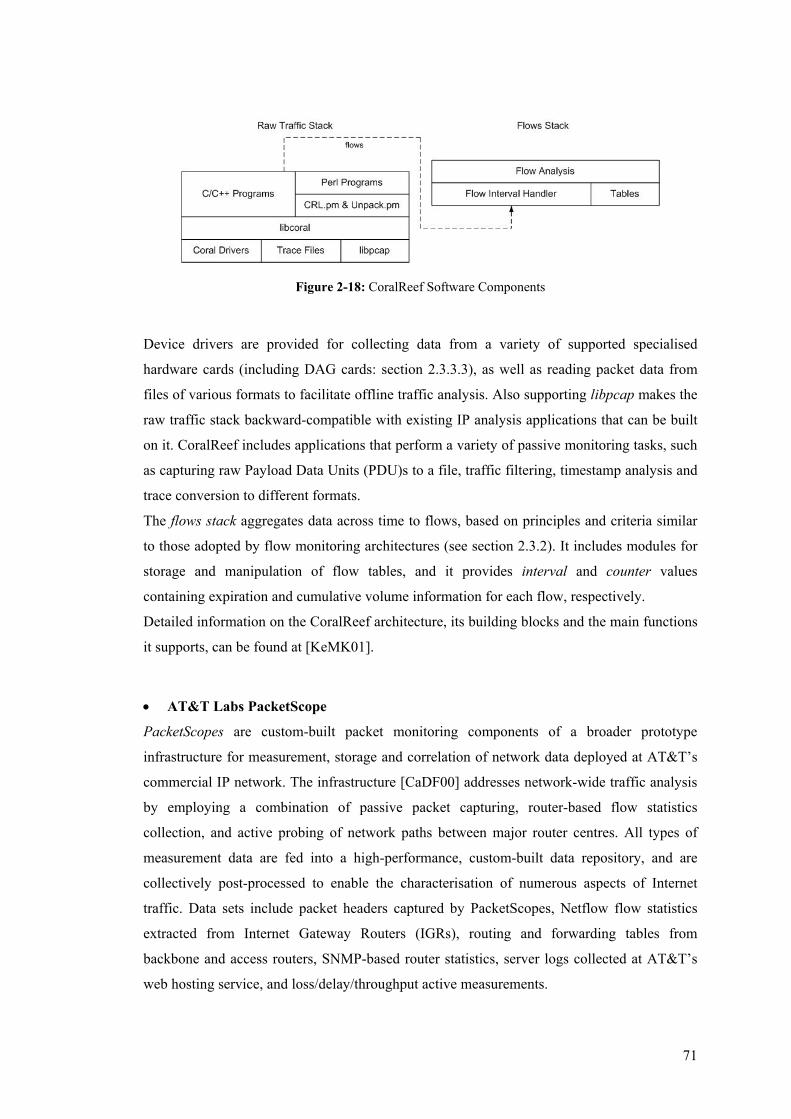
71

Figure 2-18: CoralReef Software Components

Device drivers are provided for collecting data from a variety of supported specialised

hardware cards (including DAG cards: section 2.3.3.3), as well as reading packet data from

files of various formats to facilitate offline traffic analysis. Also supporting libpcap makes the

raw traffic stack backward-compatible with existing IP analysis applications that can be built

on it. CoralReef includes applications that perform a variety of passive monitoring tasks, such

as capturing raw Payload Data Units (PDU)s to a file, traffic filtering, timestamp analysis and

trace conversion to different formats.

The flows stack aggregates data across time to flows, based on principles and criteria similar

to those adopted by flow monitoring architectures (see section 2.3.2). It includes modules for

storage and manipulation of flow tables, and it provides interval and counter values

containing expiration and cumulative volume information for each flow, respectively.

Detailed information on the CoralReef architecture, its building blocks and the main functions

it supports, can be found at [KeMK01].

• AT&T Labs PacketScope

PacketScopes are custom-built packet monitoring components of a broader prototype

infrastructure for measurement, storage and correlation of network data deployed at AT&T’s

commercial IP network. The infrastructure [CaDF00] addresses network-wide traffic analysis

by employing a combination of passive packet capturing, router-based flow statistics

collection, and active probing of network paths between major router centres. All types of

measurement data are fed into a high-performance, custom-built data repository, and are

collectively post-processed to enable the characterisation of numerous aspects of Internet

traffic. Data sets include packet headers captured by PacketScopes, Netflow flow statistics

extracted from Internet Gateway Routers (IGRs), routing and forwarding tables from

backbone and access routers, SNMP-based router statistics, server logs collected at AT&T’s

web hosting service, and loss/delay/throughput active measurements.

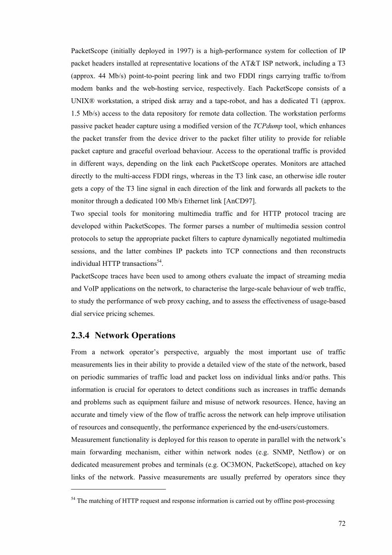
72

PacketScope (initially deployed in 1997) is a high-performance system for collection of IP

packet headers installed at representative locations of the AT&T ISP network, including a T3

(approx. 44 Mb/s) point-to-point peering link and two FDDI rings carrying traffic to/from

modem banks and the web-hosting service, respectively. Each PacketScope consists of a

UNIX® workstation, a striped disk array and a tape-robot, and has a dedicated T1 (approx.

1.5 Mb/s) access to the data repository for remote data collection. The workstation performs

passive packet header capture using a modified version of the TCPdump tool, which enhances

the packet transfer from the device driver to the packet filter utility to provide for reliable

packet capture and graceful overload behaviour. Access to the operational traffic is provided

in different ways, depending on the link each PacketScope operates. Monitors are attached

directly to the multi-access FDDI rings, whereas in the T3 link case, an otherwise idle router

gets a copy of the T3 line signal in each direction of the link and forwards all packets to the

monitor through a dedicated 100 Mb/s Ethernet link [AnCD97].

Two special tools for monitoring multimedia traffic and for HTTP protocol tracing are

developed within PacketScopes. The former parses a number of multimedia session control

protocols to setup the appropriate packet filters to capture dynamically negotiated multimedia

sessions, and the latter combines IP packets into TCP connections and then reconstructs

individual HTTP transactions54.

PacketScope traces have been used to among others evaluate the impact of streaming media

and VoIP applications on the network, to characterise the large-scale behaviour of web traffic,

to study the performance of web proxy caching, and to assess the effectiveness of usage-based

dial service pricing schemes.

2.3.4 Network Operations

From a network operator’s perspective, arguably the most important use of traffic

measurements lies in their ability to provide a detailed view of the state of the network, based

on periodic summaries of traffic load and packet loss on individual links and/or paths. This

information is crucial for operators to detect conditions such as increases in traffic demands

and problems such as equipment failure and misuse of network resources. Hence, having an

accurate and timely view of the flow of traffic across the network can help improve utilisation

of resources and consequently, the performance experienced by the end-users/customers.

Measurement functionality is deployed for this reason to operate in parallel with the network’s

main forwarding mechanism, either within network nodes (e.g. SNMP, Netflow) or on

dedicated measurement probes and terminals (e.g. OC3MON, PacketScope), attached on key

links of the network. Passive measurements are usually preferred by operators since they 54 The matching of HTTP request and response information is carried out by offline post-processing

73

monitor the operational traffic of the network, and they can hence be used with high

confidence for tasks such as network planning and dimensioning, as well as for accounting

and billing services. Active measurement techniques are often complementarily used,

however, since they operate on additionally generated (synthetic) traffic, there is an inevitable

uncertainty that any generalised assumption of applicability of results to the actual network

traffic flow will be to some degree hypothetical.

Operators responsible for managing and engineering individual Autonomous Systems (AS)s

are mainly interested in network-wide representations of the traffic, in order to drive network-

wide control actions, such as routing changes, traffic classification, traffic filtering and

capacity planning [GrRe02]. In contrast, passive traffic measurements are single-point,

operating either on a single link or being enabled on selected devices in the network. In the

latter case, measurement-enabled forwarding devices (e.g. Netflow-enabled routers) are

usually at the edges of the network, avoiding complexity and overhead at the core, where

routers need to forward large amounts of aggregate traffic.

Figure 2-19: Path, Traffic, and Demand Matrices for Network Operations

As shown in Figure 2-19, there are three main network-wide traffic representations that can be

derived by post-processing and correlating single-point passive measurements at different

granularity levels, and estimating the corresponding matrices of the flow of traffic through an

AS [GrRe02]. The path matrix specifies the temporal data volume for every path in the AS

between every ingress and egress point, and represents the current state and behaviour of the

network. The traffic matrix reveals the offered load of the network, by specifying the data

volume per ingress-egress pair. Finally, the demand matrix expresses the volume of load

originating from each ingress link and destined to a set of egress points [FeGL00].

A variety of network operations tasks can be based on populating each one of these traffic

representations. Exemplarily, the path matrix can be used to determine the traffic intensities

associated with each path in a network and to diagnose causes of congestion. The traffic

matrix can be used to generate reports for customers based on the traffic volumes between the

corresponding pairs of access links. The demand matrix can capture and predict how routing

74

affects the traffic travelling between domains. The evolution of path, traffic and demand

matrices can be exploited to identify potential bottlenecks and guide capacity planning at

longer timescales, and to tune intra-domain routing to alleviate congestion [GrRe02,

FeGL01].

However, network-wide traffic representations can be very large objects and would only

partially be populated in practice. In addition, the degree of measurement granularity is

inversely proportional with their efficient, uniform and cost-effective deployment throughout

an AS. For example, SNMP is widely implemented within network equipment to provide

aggregated information about link load, but routers usually provide relatively limited, coarse

grained load statistics. Measurement support at a finer granularity through e.g. RMON and/or

flow measurements is very costly and not available on high-speed backbone links.

Consequently, sufficient data through fine-grained, direct measurements (possibly on every

link in a large network) which could potentially fully instantiate path, traffic and demand

matrices is typically prohibitively expensive. Research therefore focuses on populating

network-wide models by estimating traffic representations, based on partial measurement

information, aggregate traffic statistics and simplifying assumptions about certain traffic

characteristics and network topology. Such studies are often referred to as network

tomography and traffic mapping, and can be overly complex involving several theoretical and

practical orientations; their discussion is outside the scope of this thesis [VaGr03, MeTS02,

CaDV00].

Practical systems addressing network operations are mainly focused on specific tasks that can

be accomplished given the instrumentation of the network and the granularity of the

measurement information available. As an example, one can consider a study within AT&T

Labs which focused on the development of an infrastructure for traffic engineering within IP

backbone networks. NetScope55 is a prototype system that consists of a set of software tools to

manage the performance of backbone topologies (AS), by generating global views of network

configuration and usage data collected from individual network elements [FeGL00]. These

can be used to visualise the network-wide implications of local changes in traffic,

configuration and control. Very briefly, NetScope consists of a set of configuration,

measurement, routing model, and visualisation modules, and a data model to combine all the

diverse attributes of network links and nodes that are derived mainly from the first two

modules. The configuration module extracts network-wide information from the configuration

files of each router in the AS, and the measurement module determines traffic demands based

55 Later renamed to Backbone Routing Analysis, Visualisation and Optimisation (BRAVO)

75

on detailed measurements at the periphery (edges) of the network56. The routing model

module combines the network topology and traffic demands to model how traffic would travel

through the AS, and the visualisation module mainly displays the layer-three and layer-two

connectivity of the network. NetScope is advertised as an extensible (distributed) and

powerful platform for “what-if” traffic engineering investigations, by providing a simulated

environment for experimenting with changes in network configurations, such as e.g. the

optimisation of intra-domain routing based on the underlying topology and traffic demands

[FeGL00].

2.3.5 Need for Sampling

The rapidly increasing data rates of communication networks impose growing measurement

demands in both processing and storage capacity, especially for finer-grained techniques, such

as flow measurements and packet monitoring. For example, it has been reported that software-

based Netflow running on high-speed routers that implement forwarding in hardware, can

cause significant overhead due to unusually large increase in CPU utilisation [NFLP].

Furthermore, the approximately 50 MB of storage requirement for daily SNMP statistics

collected over the T1 NSFNET backbone [ClPB93b], and the more than 650 MB 24-hour-

long packet trace for a single entrance interface into the T3 NSFNET backbone in 1993

[ClPB93c], have evolved -in less than a decade- to the 1.2 TB of disk space required for a 24-

hour-long trace from 11 IPMON systems over the Sprint backbone network [FrDL01].

Passive measurements are inherently more dependent (than active) on such efficiency and

performance constraints, since they operate under uncontrolled conditions, by monitoring the

non-stationary operational traffic of the network. Additionally, their seamless operation is

particularly desirable when the network exhibits extreme or abnormal conditions, and these

constraints are even more stringent.

At the finest measurement granularity level, packet monitors employ three main techniques to

reduce the processing load and the volume of measurement data: Packet filtering enables only

capturing a specific subset of packets, mainly based on the fields of the network and transport

layer headers. Partial byte capture is used to only record a limited number of bytes for each

packet, usually containing the most valuable network and transport layer headers’

information. Finally, packet sampling can be performed to limit the fraction of packets that

need to be captured and further processed. While packet filtering and partial byte capture can

provide for reduction in data volume and storage requirements, they can only marginally

decrease the per-packet processing overhead, since they still have to process in detail the

56 PacketScopes (section 2.3.3.4) have also been used within NetScope to provide fine-grained packet

monitoring data for a set of network operations tasks [CaDF00].

76

internals of every packet observed on the link. In contrast, packet sampling can also greatly

reduce the amount of per-packet overhead, and can hence be used to improve the scalability

and performance of real-time network measurement and operations. This is particularly

crucial for monitoring functions that are enabled on forwarding elements of the network. For

example, Sampled Netflow is highly recommended for high-speed routers’ interfaces since it

keeps the measurement overhead low, by allowing most packets to be switched faster without

additional NetFlow processing.

Sampling algorithms heavily depend on the application domain so, for example, we briefly

referred to algorithms targeted at identifying and keeping state for only large flows on

Netflow-enabled devices (section 2.3.2.2).

Early studies applied different sampling methodologies to single-point packet monitoring

data, and tried to evaluate the accuracy and resemblance of sampled traffic characteristics to

the characteristics of the parent population (i.e. the overall traffic volume seen on the

particular link for a specified time interval). Packet sizes and packet inter-arrival times were

among the most popularly used assessment targets, and a number of statistics have been used

to indicate similarity between the sampled and the parent distributions [ClPB93c, AmCa89].

Three classes of sampling schemes that have been widely considered are the systematic

sampling, stratified random sampling and the simple random sampling. For any one of these

classes, particular sampling fractions can be implemented using either event-based or timer-

based mechanisms. Hence, packet counters or timers can trigger the selection of a packet for

inclusion in the sample.

Systematic sampling describes the process of deterministically selecting every kth element of a

trace. The process configures its granularity by selecting the starting points and the duration of

the selection intervals. A systematic sampling algorithm can select every nth packet arriving at

a monitored interface, or all packets arriving at pre-defined time intervals (e.g. select one

packet every U seconds). Stratified random sampling is similar to systematic and it describes

the process of randomly (rather than deterministically) selecting an element from within a

specified subset of the parent population. The elements of the parent population are first

grouped into subsets in accordance to a given characteristic (time or counter-based). Then, an

element from each subset is selected at random (e.g. randomly select a packet from within

each 30 second interval of a trace). Simple random sampling describes the process of

randomly selecting k elements from the total population. Random sampling requires the

generation of random numbers, and can achieve unbiased estimators by avoiding using strict

periodic descriptors that might resemble possible periodic characteristics of the observed

phenomenon. Random sampling is considered to be the most dependable representation of the

parent population, but it imposes greater implementation cost in obtaining the random value.

Packet count-triggered sampling techniques have been reported to perform better than time-

77

triggered ones, especially for assessing packet inter-arrival times, mainly due to the frequent

bursty periods when many packets arrive on a link with small inter-arrival times (often missed

by timer-based sampling) [ClPB93c].

2.3.5.1 Trajectory Sampling

More recently, a highly-cited study suggested packet-content-triggered sampling by matching

the invariable contents of a packet against a hashing function to select a representative sample

of traffic across a measurement domain. Trajectory sampling [DuGr01] is a method for

network-wide (multi-point) packet sampling, and provides an estimator for the path matrix

through direct traffic observation. Instead of randomly sample packets at each link, this

method makes a sampling decision based on a deterministic hash function over the packet’s

content and hence, by using the same hash function across a domain to sample packets, it

ensures that a packet is either sampled on every link or on no link at all. The hash function,

although deterministic, it resembles a random sampling process, so that the subset of sampled

packets are not statistically biased in any way. When a packet is selected to be sampled, a

second hash function is used to obtain a unique packet identifier (label) within the domain,

based again, on the packet’s content. Each link within the domain that selects a packet to

sample, it then computes a label which is sent to a measurement system. By matching labels

generated from different links in the domain, the path that a packet followed from ingress to

egress can be inferred. The uniqueness57 of labels generated for different packets within a

measurement period, as well as the degree of pseudo-randomness of the sampling process

both depend on choosing the appropriate hash functions.

Implementation of this, network-wide, trajectory sampling requires that each link interface is

capable of computing both the sampling and the label hashes. However, it does not require

router state other than a small label buffer, and it is claimed that it can be implemented using

state-of-the art Digital Signal Processors (DSP)s even for the highest interface speeds

available today. In addition, the label generated for each sampled packet in each interface that

then needs to be transferred to a measurement system for correlation and post-processing can

be as small as 20 bits. By being a direct traffic measurement method, trajectory sampling does

not require any status information from the network, and can produce a sample of the path

matrix that dynamically adjusts to alterations in the traffic flow of the network.

57 Some identical labels can be disambiguated to unique trajectories, depending on the network

topology and the traffic rates on all other trajectories

78

2.3.5.2 The IETF Packet SAMPling (PSAMP) Working Group

Within the Internet community, the IETF’s Packet SAMPling (PSAMP) Working Group has

relatively recently been established to define a standard set of capabilities for network

elements to sample subsets of packets by statistical and other methods. Sampling capabilities

should be computationally simple in order to be implemented ubiquitously at maximal line

rate, but at the same time, they should be able to support a range of existing and emerging

measurement-based applications [PSAM].

The main objective of the working group is to standardise the way a fraction of traffic can be

sampled, collected and transported as opaque objects under three main processes. A selection

process inspects each packet at an observation point to determine whether it should be

sampled. Observation points can be a shared medium, a single port of a router, or a point-to-

point link to which a probe is attached. Selection process can maintain state information by

updating variables such as packet sequence numbers and arrival timestamps. A packet can be

sampled based on the packet content, on information derived from packet’s treatment at the

observation point, or on any state information maintained by the selection process. A

reporting process constructs a report stream on packets selected by the selection process, in

preparation for export. Packet reports can contain a subset of the packet content, together with

selection state and packet treatment information. An exporting process sends, in the form of

export packets, the reports collected from one or more selection/reporting processes to one or

more collectors [Duff05]. Interestingly, it has been suggested that the IPFIX protocol (section

2.3.2.3) will be used for export of the report stream.

A PSAMP device should host at least one observation point and an instance of a selection, a

reporting, and an exporting process.

The PSAMP working group targets at specifically providing standards for the exact packet

information that should be available for reporting, the exact format of the report constructed

by the network element, the format of the stream of the packet reports, as well as the interface

for presentation of reports to on-board applications. Additionally, the definition of a packet

sampler MIB to include parameters for packet selection, packet report and stream format is

scheduled, which can potentially increase the popularity and widespread deployment of

PSAMP functionality within SNMP agents.

2.4 Summary An in-depth survey of the major deployments and advances in network and Internet

measurement has been presented in this chapter. Active and passive measurements are the two

broad categories, under which measurement techniques, infrastructures, and tools have been

classified. Their main conceptual difference is that active measurements generate additional

79

synthetic traffic and assess its perceived performance as part of a direct measurement process,

whereas passive measurements mostly monitor, record, and analyse existing (operational)

traffic on network links and nodes without (negatively) impacting the network.

Active measurements have been decomposed down to different categories depending on the

protocols (and hence the mechanisms) they use to probe the network and measure its response

to certain stimuli, and major representative deployments of each category have been described

in detail. In addition, the direct implementation of specific performance metrics by active

measurement techniques and their consequential coupling have been identified, and recent

efforts for standardising performance metrics within the Internet community have been

documented.

Passive measurements have been categorised based on the granularity of the measurement

process with respect to the level of detail of monitored data, from aggregate properties of

network links and nodes, to fine-grained details of flows and individual datagrams.

Representative tools and techniques have been presented, as well as related standardisation

activities. The coupling of passive measurement techniques with network operation activities

and the need for data reduction through sampling and targeted measurement have also been

raised and briefly discussed.

80

Chapter 3

3In-Line Service

Measurements and IPv6 3.1 Overview The preceding chapter focused on a thorough discussion regarding the deployments and

advances in network traffic measurement techniques, and provided a detailed taxonomy of

representative developments under the two major streams of active and passive network

measurement, also describing their relative capabilities. This chapter critically presents the

main limitations imposed by the inherent characteristics of active and passive measurements,

and also by particular realisations within each broad measurement category.

In-line measurement is then introduced, which is a new measurement technique that exhibits

hybrid properties with respect to active and passive measurements, and is capable of

accurately determining the perceived performance of operational traffic flows, through a

direct multi-point measurement. In-line measurement seeks minimal cooperation from

network nodes, and uses extension header fields of the next generation Internet Protocol

(IPv6) to encode measurement indicators within the actual network traffic data units, at the

ubiquitous network (IP) layer. The exploitation of native IPv6 mechanisms to provide for a

pervasive measurement plane capable of assessing the otherwise immeasurable performance

properties and service response experienced by virtually any type of operational traffic is

discussed and advocated. The advantages of the in-line, IPv6-based measurement technique,

are raised and elaborated, and the definition of two measurement TLV-encoded options to

implement a number of timestamping and packet sequencing-related metrics is then provided.

The chapter concludes with a discussion on the flexibility and the different realisation

scenarios of the in-line measurement technique, and on the great potential of such

measurement instrumentation mechanism for next generation IP networks.

81

3.2 Limitations of Active Measurement Techniques As it has been described in the previous chapter, active measurement techniques mainly

consist of software programs that use the network and then try to analyse its performance

through direct measurement observation [Paxs98b]. The different service quality metrics

commonly assessed by directly measuring the network’s response to the injected stimulus can

include end-to-end delay, packet loss, bulk throughput, end-to-end path properties, and

bandwidth characteristics; numerous performance metrics are being standardised within the

IETF’s IPPM working group [IPPM].

Active measurements can give insight into network conditions by tuning and calibrating

specific measurement processes. However, due to the generation of specific types of traffic,

based on which measurements are conducted, active measurement techniques suffer the

inherent limitation of only being able to measure the performance experienced by this special-

purpose traffic during the measurement interval. This property can be an advantage at the

same time, since the measurement process is fine-grained, able to target at specific types of

flows and services. However, the synthetic traffic’s performance might not reflect the overall

performance characteristics of the network between the instrumented end-points, and

moreover, it might not reflect the performance experienced by the different types of

operational network traffic. Measurement processes based on ICMP or otherwise uniquely

identifiable IP traffic (e.g. based on dedicated transport-level measurement protocols) cannot

provide convincing evidence that their performance indications reflect the service quality

characteristics of user IP traffic, carried on top of other common transport mechanisms such

as TCP and UDP. At the same time, transport-oriented measurement processes based on

traffic carried on top of a particular transport mechanism (e.g. TCP or UDP), cannot assess the

performance of traffic carried over different transport mechanisms, nor can they control how

the measurement traffic interacts and multiplexes with other traffic, even of the same transport

mechanism58.

ICMP-based active measurements mainly suffer from the special response and treatment that

ICMP packets might elicit from the network (across and within Autonomous Systems). It has

been repeatedly reported that ICMP packets can be given different priority than the rest of the

operational network traffic, either by deliberate filtering, or by QoS techniques being enforced

on network nodes [MaCo00a, CoLW03, Benn03]. Network operators can give lower or even

higher priority to ICMP packets from the rest of the traffic, in order to minimise their impact

58 As an example, early studies on TCP showed bias against connections passing through multiple

congested gateways, bias against connections with longer round-trip times, and bias against bursty

traffic [Floy91].

82

on the network or to make the network appear to be offering a better service than it actually

does, respectively (although the latter phenomenon has been rarely reported in practice). At

the same time, QoS strategies deployed on access AS routers can give ICMP packets lower

priority in order to increase the performance of other types by giving higher priority to TCP

and UDP packets [MaCo00a]. Core network nodes can be configured to even drop ICMP

packets and not processing them at all, due to extreme performance constraints imposed by

the forwarding of large amounts of aggregate traffic. Additionally, the use of ICMP packet in

certain types of security attacks has made operators to often block ICMP packets from

entering their networks. Rate limiting of ICMP packets has also been observed especially in

networks with low-bandwidth connections. Once the amount of ICMP traffic has reached a

specified limit, further ICMP packets are dropped. If blocking is relatively easy to detect, the

dynamic nature of rate limiting can potentially lead the measurement process to great

uncertainties, since it makes it harder to infer whether losses have occurred due to network

conditions or administrative policies. This distinction is particularly difficult to make when

the measurement process consists of small periodic bursts of ICMP packets. Both blocking

and rate limiting of ICMP traffic have been reported to increase, especially in developing

countries, which consequently makes the accuracy and universal applicability of ICMP-based

measurements even more questionable [CoLW03].

Also, ICMP measurements mainly measure the round-trip properties of an instrumented path

through systems’ echo responders. The observation usually takes place at a single point in the

network that generates an ICMP echo request message, receives a corresponding echo reply

from a target system and computes round-trip time and loss figures. However, this

measurement does not directly give insight on which direction of the path is responsible for

the observed phenomena. Not only the two directions of an Internet path can experience

different levels of performance, but in some cases they might even be physically different, due

to routing asymmetries and dynamic re-configuration. Hence, the behaviour of round-trip

delay and loss figures cannot be safely decomposed down to its unidirectional contributors.

Studies have shown that the approach of dividing round-trip latencies by two to derive their

one-way decomposition is of questionable accuracy [ClPB93a].

Dedicated measurement protocols that operate directly on top of IP59 inherit most of the

limitations of ICMP-based measurements regarding the relevance of the results to the

operational network traffic. Protocols like the IPMP (section 2.2.5) can actually be

characterised as measurement-oriented enhanced versions of ICMP [LuMB01]. They deploy

echo request-reply mechanisms similar to ICMP, but their header fields are defined to provide

space for carrying more extensive and informative measurement data. Hence, for example,

59 Like ICMP, these protocols operate at the IP layer

83

IPMP packets can carry path records identifying all the network nodes a packet has visited,

and also provide space for a 64-bit timestamp to be inserted at each node. IPMP is designed to

measure one-way metrics and can therefore overcome the uncertainties introduced by round-

trip measurements. However, the main limitation influencing the accuracy of ICMP-based

measurements also applies to dedicated measurement protocol traffic. That is, the

measurement traffic is still visible, this time uniquely identified by a distinct IP protocol

number. Operators and QoS enabling techniques can still manipulate, filter, and rate limit the

measurement traffic, as it is the case today with ICMP traffic. Therefore, the relevance

between the network response experienced by the measurement traffic, and that experienced

by the operational user traffic, remains highly questionable. Additionally, such dedicated

measurement protocols do not follow the basic principle of most traditional active

measurements, which is to exploit existing network mechanisms to measure traffic

characteristics. They instead introduce features60 whose full exploitation would require all

network nodes to implement such measurement functionality on their forwarding paths;

something that is very difficult to be practically realised today, mainly due to the multi-vendor

nature of the Internet but also due to the incurred overhead on high-speed nodes.

TCP and UDP-based active measurements exhibit a higher probability of revealing the

service quality characteristics experienced by certain portions of the operational network

traffic. It can be claimed that a measurement process that operates on top of general-purpose

transport mechanisms can resemble the performance characteristics of similar operational

traffic, carried over the same portions of the Internet infrastructure, during the measurement

time interval. Most transport-based measurement infrastructures (section 2.2.4) encapsulate

their injected traffic within small and medium-sized61 UDP datagrams, which gives more

control to the application in choosing the desired packet size distribution and packet sending

rates. However, due to the absence of end-to-end congestion control for the UDP traffic, the

performance experienced by the UDP-based test-traffic will not necessarily reflect the

performance experienced by the dominant TCP-based operational network traffic, nor that

experienced by other, competing UDP flows over the instrumented network path. During

periods of high network load, the unresponsiveness of UDP traffic to congestion indications

60 For example, IPMP is intended to store full trace information for its packets, reporting every visited

network node’s IP address, together with the corresponding arrival/departure time. Currently, since the

Internet consists of non-IPMP capable nodes, its minimal implementation can only measure end-to-end

one-way metrics between instrumented end-points, similar to the ICMP timestamp request and

response messages. 61 UDP-based test traffic packets are usually between a few tens and a few hundreds of bytes long.

84

can result in bandwidth starvation of competing TCP flows, whose goodput62 can greatly

decrease due to backing-off in response to packet drops. At the same time, the goodput of

UDP flows can stay nearly constant, falsely reporting a better level of service that the network

actually delivers [FlFa99]. Competing UDP flows can also experience randomly different

performance than that reported by the UDP-based test traffic, depending on their sending

rates, the queuing disciplines enforced at nodes along the path, and the load of the network

during the measurement interval. Additionally, due to this unresponsiveness to congestion,

rate limiting can also be enforced to UDP traffic during periods of peak network usage,

victimising63 the accuracy of the (UDP-based) measurement results [LuMB01].

The dominant presence of TCP on the Internet, together with the aforementioned concerns64

incurred by ICMP and UDP-based measurements has led some researchers to use TCP-based

test traffic to analyse network performance. The end-to-end performance observed by TCP

transfers can match closely the service experienced by the users of the network. However, the

TCP protocol behaviour is complex and in the presence of different TCP implementations on

different end-systems, it proves difficult to determine which facets of the overall connection

behaviour are due to the state of the network path, and which are due to the behaviour of the

TCP implementations at the end-points [Paxs97b]. Also, the complex and CPU intensive

operations65 within systems’ TCP stacks introduce additional components (mainly) of delay

which are difficult to distinguish from genuine network pathologies [LuMB01]. The reliable

stream transport service provided by TCP demands data to be exchanged in both directions of

an individual connection. TCP’s data (forward) path adapts the rate it transmits packets based

on previously observed network conditions, hence the data packets do not reflect an unbiased

measurement process. On the other hand, the reverse path consists of small acknowledgement

packets whose transmission does not adapt to the network path’s conditions, and hence

reflects a cleaner measurement process [Paxs97b]. The different characteristics of the traffic

in the forward and reverse TCP paths, the way the performance experienced by the test-traffic

over each path relates to the performance of the operational traffic, as well as the required

knowledge of the internals of individual TCP implementations, makes the use of TCP by

infrastructures for scheduled test-traffic measurements a challenging task.

62 Here, we use the definition of goodput from [FlFa99]: The goodput of a flow is the bandwidth

delivered to the receiver, excluding duplicate packets. 63 With side-effects similar to those experienced by ICMP-based traffic/measurements 64 A shared concern between ICMP and UDP-based measurements is the rate at which probes are sent:

There is a trade-off between overloading a network path and probing conservatively with no possibility

of analyzing finer time-scales [Paxs97b]. 65 For example, matching arriving packets with the corresponding data structures.

85

In addition to the aforementioned specific limitations encountered by the different active

measurement methodologies, there exist two fundamental limitations applicable to active

measurements in general, regardless of the individual mechanisms deployed. The first is that

the injection of additional test-traffic into the network, especially at application-configurable

rates, might itself be a factor of performance degradation, sometimes creating an additional

load and consuming a considerable amount of network resources, and at the same time

competing with the operational network traffic66. Hence, the measured levels of network

performance can to some extent be attributed to the presence of the test-traffic in the network.

Secondly, the periodic sampling used by most infrastructures to inject measurement traffic in

the network at regular intervals can lead to inaccuracies in the measured performance, by

either failing to observe periodic network events that occur at times other than when the

samples are scheduled, or by synchronising with events occurring regularly just as the samples

are scheduled67 [MaCo00a].

3.3 Limitations of Passive Measurement Techniques Passive measurements attempt to characterise aspects of traffic behaviour by monitoring the

existing, operational load and the traffic dynamics of the network. Having their origins in

traditional network element management, these techniques employ a combination of hardware

and software processes that are either integrated into network nodes or physically attached to

individual network links, and they operate in parallel with the main forwarding mechanisms of

the network. Monitoring the operational status of a portion of the network is the main

undertaken activity, whereas making conclusive measurements of the network service can be

an afterthought, or an offline, separate process. Monitoring data can prove tremendously

valuable in revealing long term trends of traffic and network behaviour, however, the

infeasibility of real-time measurement analysis is a constraining factor for revealing the

service quality properties of operational traffic at finer time scales. At different granularity

levels, the common theme of passive monitoring systems is that they require access to the

network infrastructure and that they are autonomously deployed at a single point in the

network. Access to the infrastructure is a serious constraint, since its political implications

66 A mismatch between the injected test-traffic’s sending rate and the capacity of the instrumented path

can result in the measurement traffic grossly overloading the network [Paxs97b]. 67 This synchronisation can result in the network appearing to deliver a better or poorer performance

than it actually does. In order to observe an unbiased sample of network conditions, Poisson [PaAM98]

and exponential [Paxs97b] distributions of sampling intervals have been suggested.

86

limit the scope68 of passive measurement within a single administrative domain. Coupled with

the consequential privacy issues that occur due to the monitoring of the actual traffic, this

leads to the following controversy: although passive measurement systems monitor the

operational traffic flows, they are inadequate of targeting the service experienced by the actual

(end-to-end) application traffic; what they can ultimately measure is an approximation of the

service offered by a single “network cloud”, as seen from an operator’s (and not end-

user/application’s) perspective. Operating at a single point in the network allows passive

techniques to monitor data and update relevant counters at certain network nodes and links.

However, correlating such partial information from multiple monitoring points to reveal the

performance of traffic carried between two (or more) Points-of-Presence (POPs) in the

network is a computationally challenging task, that consumes vast amounts of processing and

network resources, and cannot be undertaken in real-time. Moreover, instantiating network-

wide traffic models relies on several assumptions and heuristics about the network, the traffic,

or both, since the required levels of direct measurement observation and correlation would be

prohibitively expensive [GrRe02, MeTS02].

SNMP is widely implemented into network nodes and adopts an element-centric view of

network management, primarily focusing on reporting the operational status of the network

elements, preventing and isolating fault conditions, and restoring normal operation in case of

equipment failures. Even the traffic-related variables maintained by SNMP agents (which can

give some insight into the operational conditions of particular network interfaces and links)

only maintain counters describing statistics relevant to the implementation and execution of

parts of the networking stack at a node, and not how they relate with the actual traffic flows

and their properties [Stal99]. RMON provided a great enhancement for SNMP, facilitating

remote and distributed monitoring of LANs. It can ideally provide for high-level traffic

statistics and filtering mechanisms tuned to monitor specific traffic flows and packets. In fact,

it has been stated that if RMON were universally deployed, the need for additional packet and

flow monitoring support would be obviated. However, their implementation is so costly and

infeasible for high-speed backbone interfaces that they can only be partially realised at low-

speed router interfaces, and hence be relegated at the edge of the network [GrRe02]. As they

stand, SNMP and RMON implementations can give useful information about the amount of

68 Actually, network operators’ political and business-oriented issues can be claimed to be the most

constraining factors for passive traffic measurement. The level of network performance or the Traffic

Engineering (TE) policies and activities are details an operator would not normally want to share with

their competitors. Such political issues are noted here, however the focus of this thesis is on the

technical capabilities (and limitations) of the different measurement techniques.

87

data flowing across an administrative domain, yet they cannot give a detailed view of the

traffic and the way it behaves [Brow99a].

Flow-level passive measurement systems are either deployed within network nodes or are

attached to network links, and create the abstraction of the flow to measure several properties

of groups of packets, at the same time limiting the amount of required resources and offline

processing. In doing so, they can compute aggregate statistics for basic traffic characteristics

such as average packet sizes, traffic volumes per IP addresses/ports/protocols, but they do not

provide fine-grained timing information about individual packets and cannot study properties

of network traffic at a small time scale [GrRe02]. The most popular flow measurement tools

are router-based enhancements and hence suffer from scalability, due to the need of keeping

flow state in the routers. Unlike SNMP-based techniques that only keep and update a standard

set of counters, flows can be defined in different aggregation levels and the number of

concurrent flow entries can seriously constraint the resources of the network node. Sampling

is being used to alleviate this overhead problem, but it obviously affects the measurement

accuracy.

At the finest level of measurement (data collection) granularity, packet monitoring systems

are usually attached to key network links and capture the main operational data-units

(packets). They are arguably the most traffic-characterisation-oriented passive measurement

technique, since their operation is not determined and/or constrained by the network nodes

(router-imposed limitations). They can keep measurement data for every packet observed on a

link and they can analyse it in different ways to give insight into different aspects of traffic

behaviour. Packet monitors suffer from the continuously increasing network speeds in two

main ways: first, collecting traces at high-speed links almost certainly requires dedicated

optimised hardware equipment support. And second, although keeping pace at increasing link

speeds can be currently accommodated by advances in the corresponding hardware

monitoring equipment, the increasing volume of measurement data that will eventually need to

be analysed is another major limitation. This latter difficulty is attempted to be tackled by

traffic filtering, packet sampling and by capturing only a limited number of bytes per packet.

However, all these techniques can result in accuracy limitations themselves. A conceptual

constraint of packet monitoring is that due to its single-point nature it is difficult to be tuned to

measure traffic-perceived performance even across a single administrative domain. The

implementation of even the simplest service-oriented performance metrics (such as those

defined within the IPPM working group –section 2.2.2) require measurements to be conducted

at (at least) two distinct points in the network69. Such performance measurements can be

69 Passive monitoring systems have mainly focused on analysing one-point traffic attributes, such as

packet size distributions and packet inter-arrival times at backbone Internet links. Metrics that show

88

achieved by correlating two single-point measurement traces, yet this correlation is a very

costly and uncertain task. The amount of monitored data that needs to be transferred across

the network to be analysed can be very large70 (especially when multiple traces are correlated)

and it often needs to be carried over dedicated network links. Correlation and analysis of the

traces is therefore an offline, computationally challenging activity. Targeting specific services

and flows is difficult and uncertain, especially if any of the (monitoring) data-reduction

techniques have been used71. Most sampling algorithms72 would not guarantee that the same

packet is sampled at more than one point in the network. The less bytes-per-packet are being

captured by the monitor, the less distinguishable packets become and the more likely it is for

packets to be mismatched during correlation.

Overall, passive measurement techniques can provide accurate indications of certain aspects

of the operational traffic, and they can provide operators with valuable information of network

and traffic behaviour in relatively broad time scales. However, their main general limitation is

that they cannot extend across AS boundaries, and they do not assess the levels of service (as

these are described by commonly adopted performance metrics) experienced by the traffic

through a domain, in finer time scales. Additionally, passive measurement techniques that are

integrated in network nodes are usually governed by lengthy standardisation processes and

hence impose constraints upon independent, open-ended experimentation.

3.4 In-Line Measurements: A New (Hybrid) Measurement

Technique The thorough analysis of the existing measurement techniques has made it clear that they have

different advantages and limitations, and they have been used for different purposes so far.

The focus of active measurements has been on providing insight into the effects of network

problems on users, whereas passive measurements have mainly used post-analysis to

determine the causes of network performance problems [VaEs04].

It has become evident however, that the Internet lacks a generic measurement mechanism

whose functionality can be an integral part of the Internet’s operation. In other words, the

Internet lacks a measurement plane, which would operate as part of the forwarding

how traffic is routed within a network such as, for example, one-way delay, have started gaining the

attention of recent passive monitoring studies [e.g. ChMZ04, NiMR04, DuGr01]. 70 1.1 TB of a 24 hour long measurement trace was reported in [FrDL01] 71 It cannot be absolutely guaranteed that both monitoring points trigger on the same packet. 72 Specific sampling algorithms have been developed for this exact reason: To ensure that if a packet is

sampled at one point in the network, it is then sampled at all other points (section 2.3.5.1).

89

mechanism73, and would be able to reveal the performance levels experienced by the

operational traffic accurately, un-intrusively, and in a timely manner.

The main reason for this (lack of) behaviour can be traced back in the design philosophy of

the Internet and its protocols, where resilience, scalability and interconnection of multiple

types of networks were among the primary concerns to be addressed; accountability of

resource usage only appeared last on the priority list74 of the Internet architecture’s design

goals [Clar88]. Consequently, performance measurement was an afterthought that over the

years has evolved to operate in parallel with but independently from the Internet’s operation,

in many cases competing with the operational traffic. Hence, active measurements attempt to

exploit transport and control mechanisms of the TCP/IP stack to assess the network response

elicited by additional synthetic traffic, and passive measurements deploy independent systems

that monitor traffic and post-process counter-based data to analyse only a fraction of network

performance metrics at longer timescales. Apart form individual shortcomings the general

limitation of these practices is that the measurement process is totally independent from the

Internet’s forwarding operation, and therefore sometimes measurement can be an end in itself:

The measurement results can be marginally or even questionably relevant to the actual

network response to the user traffic. Furthermore, using the measurement results as input to

operations such as traffic engineering, SLA validation, and network-wide traffic model

population, usually involves applying heuristics and making assumptions about the network,

the traffic and the routing model, and requires correlation of additional configuration data

[FeGL01, GrRe02].

The focus of this thesis is, rather than to incrementally improve some aspect of the existing

measurement approaches and/or their sub-categories, to propose a new measurement

technique that exploits network and protocol support to directly measure the performance

properties75 of network traffic for next generation IP networks.

In-line measurements are a new approach that extends the classification of the measurement

techniques, and exhibits hybrid characteristics of both active and passive approaches. The

cornerstone for the efficient realisation of in-line measurements is the exploitation of

mechanisms provided by the next generation Internet Protocol (IPNG) to define measurement

protocol extensions to be applied directly at the data path of the operational network traffic

and implement an extendible set of standardised performance metrics. Packet-level,

instantaneous measurement indicators (such as timestamps and packet counters) are carried

73 Without, of course, negatively impacting its performance. 74 We acknowledge, however, that the Internet owes much of its success to this prioritisation of goals. 75 As these are described by a variety of standardised performance metrics.

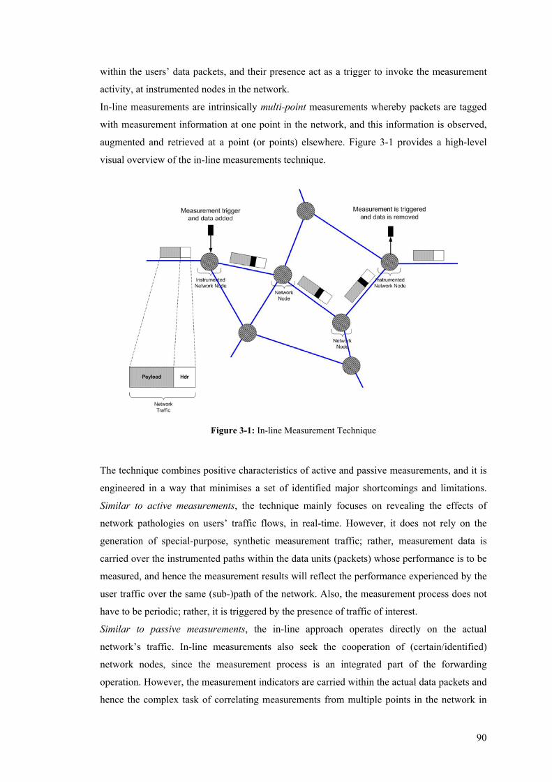
90

within the users’ data packets, and their presence act as a trigger to invoke the measurement

activity, at instrumented nodes in the network.

In-line measurements are intrinsically multi-point measurements whereby packets are tagged

with measurement information at one point in the network, and this information is observed,

augmented and retrieved at a point (or points) elsewhere. Figure 3-1 provides a high-level

visual overview of the in-line measurements technique.

Figure 3-1: In-line Measurement Technique

The technique combines positive characteristics of active and passive measurements, and it is

engineered in a way that minimises a set of identified major shortcomings and limitations.

Similar to active measurements, the technique mainly focuses on revealing the effects of

network pathologies on users’ traffic flows, in real-time. However, it does not rely on the

generation of special-purpose, synthetic measurement traffic; rather, measurement data is

carried over the instrumented paths within the data units (packets) whose performance is to be

measured, and hence the measurement results will reflect the performance experienced by the

user traffic over the same (sub-)path of the network. Also, the measurement process does not

have to be periodic; rather, it is triggered by the presence of traffic of interest.

Similar to passive measurements, the in-line approach operates directly on the actual

network’s traffic. In-line measurements also seek the cooperation of (certain/identified)

network nodes, since the measurement process is an integrated part of the forwarding

operation. However, the measurement indicators are carried within the actual data packets and

hence the complex task of correlating measurements from multiple points in the network in

91

order to implement service-oriented performance metrics is obviated. Direct measurement can

therefore be conducted in short time scales and even in real-time. At the same time, the

presence of the measurement data within the packets makes it entirely certain that the same

packet has been observed at any chosen point in the network. The remainder of this section

provides an outline of the primary requirements and goals of the in-line measurements

technique.

• Increased Accuracy and Relevance

The technique should be able to produce results that accurately reflect the performance

experienced by the operational traffic of the network. Hence, the measurement process should

not perturb the network in any way that would introduce bias to the resulting analysis.

Measurement instrumentation should be implemented in such a way so that the instrumented

traffic (carrying measurement data) is treated identically with the rest of the network traffic,

and does not elicit any special response on its journey through the network. The nature of in-

line measurements guarantees that the measured performance reflects the service experienced

by the user traffic, since measurement computation is based on indicators carried within the

actual data packets. Therefore, the major challenge is to implement the technique in such a

way, that instrumented traffic is not uniquely identified and not distinguished from traffic not

carrying any measurement data, and that it does not require any special response from all the

forwarding nodes in the network. Only nodes and/or end-systems that take part in the

measurement process should be required to conduct extra processing on the instrumented

packets. The forwarding behaviour of the rest of the nodes should not be impacted by the

presence of measurement data, in any way.

• Directly Measuring the Service

As it has been stated earlier, the goal of the in-line measurements is to reveal the effects of

network state to the service experienced by the user traffic76. The granularity of the

measurement process should be flexible and configurable. It should be feasible for in-line

measurements to measure the performance of specific services and application flows, at

different levels of granularity and aggregation. At the same time, the technique should be

general enough to be applied to any type of service, transport and application, and its

applicability should not be constrained and/or limited by specific types of traffic. Therefore,

reliance on specific transport or application-level mechanisms for the realisation of the in-line

measurements technique is not considered adequate.

76 The terms in-line measurements and in-line service measurements will be used inter-changeably in

the remainder of this thesis.

92

The direct implementation of service-oriented performance metrics yields the need for a multi-

point measurement technique, able to compute the network’s response to the operational

traffic between two (or more) points in the network.

• Minimal Impact on the Network

Both the measurement process and the measurement data should have a minimal impact on

the network’s operation. The possibility of using additional dedicated measurement traffic to

inject special stimulus (and load) into the network has hence been eliminated, since in such a

scenario it is difficult to assess the exact impact the measurement traffic has on the network’s

operation and how this impact influences the measurement results.

Since in-line measurements operate on the actual data packets of the network, the

intrusiveness of the measurement process should be minimised to only incur a marginal

additional processing delay, at only a minimum number of instrumented network nodes.

Filtering and sampling mechanisms should also be applicable to offer more control on the

intrusiveness of the measurement process.

The need for correlation of measurement data from multiple (two or more) end-points in order

to perform unidirectional measurements should also be eliminated. Only a minimal amount of

per-packet measurement indicators should be carried along the network within the data

packets, and cumulative measurement data should be generated (if needed) at one end-point of

an instrumented path.

• Applicability

Success of a measurement mechanism also lies in its potential to be widely deployed without

requiring major modifications and enhancements of the Internet mechanisms/principles,

neither at an infrastructural nor at a service level. One of the advantages of some active

measurement techniques in this respect is that they exploit mechanisms already implemented

(almost) ubiquitously across the Internet77. Likewise, in-line measurements should exploit

existing Internet mechanisms in order to target near-ubiquitous applicability while incurring

minimal operational enhancements. Being able to be deployed incrementally and at the same

time inter-operate seamlessly with the rest of the Internet infrastructure, are two important

characteristics the technique should exhibit. Additionally, flexibility as to where in the

network in-line measurements can be applied is another desirable property that can be met by

the technique not being tightly coupled with or relying on proprietary (mainly hardware)

processing systems78.

77 For example, ICMP-based measurements exploit the ICMP echo responder, which is implemented in

all (modern) networked nodes and end-systems. 78 Such as, for example, dedicated packet monitoring/measurement probes.

93

• Timely operation and cooperation with the network nodes

It has lately become evident that although current approaches to measurements problems

either assume minimal support from network nodes and protocols (e.g. active measurements)

or load routers (nodes) with heavy-weight operations (e.g. NetFlow), future measurement

solutions should consider cooperation of routers, protocols, and tools [VaEs04]. Adopting this

attitude, in-line measurements exploit protocol mechanisms and seek support from identified

nodes in the network, in order to provide for a measurement plane for the next generation

Internet that can potentially offer a ubiquitous, always-on measurement service in parallel

with the network’s forwarding mechanism. The measurement process should be direct and not

a task of post-processing analysis in order to be able to operate in relatively small timescales,

to reveal performance fluctuations in real-time, and to potentially provide input for re-active

Traffic Engineering (TE) activities [PeSS04].

3.4.1 On the Scope of the In-line Measurement Technique

The number of instrumented systems in the network that will trigger the additional per-packet

measurement processing clearly influences the scope and the operational framework of the in-

line measurement technique.

The general concept of piggybacking control indicators within the network’s data units can be

considered advantageous for several networking research disciplines. Especially in the area of

active and programmable networking research, there is considerable functionality that can be

encoded and processed en-route to provide for a variety of enhanced and customised network

services and operations. From a more specific network measurement viewpoint, control data

processing en-route can be used to reveal numerous properties of the traffic, such as among

others the route packets followed from their source to their destination and the available

capacity of Internet paths. However, such operations would require additional processing at

many different network nodes along a packet’s delivery path, and possibly at every visited

node. As it has been made clear in the previous chapter, the vast majority of measurement

techniques and infrastructures concentrate on revealing traffic performance properties either

end-to-end, or within autonomous system boundaries, and measurement activity is mainly

conducted at one or two points in the network. This is principally motivated by the desire to

only incur additional processing overhead on a minimal number of network nodes along a

packet’s delivery path, so that the measurement process (and possibly the instrumented traffic)

is not biased in any way, and it is not recording different response from the network than the

rest of the operational traffic. Likewise, since in-line measurement is designed to actively

instrument the actual network traffic, un-intrusiveness is one of the most crucial requirements

which is also tightly coupled with the accuracy and relevance of the measurement process. It

94

is envisaged that minimal additional measurement processing will take place at a well-

identified and adequately-provisioned minimum number of network nodes or end-systems.

Hence, the focus of this thesis is on the two-point instantiation of the in-line measurement

technique, either end-to-end or edge-to-edge mainly between domain ingress and egress points

of presence. As it will become evident in the following sections, the technique has been

adequately engineered so that the vast majority of the general-purpose forwarding network

nodes are not impacted by any sort of additional processing due to the presence of the

measurement indicators in the datagrams. At the same time, the possibility of measurement

activity being invoked at more than two points in the network is also mentioned, and its major

implications and applications are briefly discussed (in sections 3.9 and 3.10).

3.5 Internet Protocol: How It Was Not Designed For

Measurement In order for the in-line measurements technique to instrument with measurement data the

operational network traffic so that it accurately reveals the performance experienced by the

application flows, adequate mechanisms to seamlessly engineer such functionality have been

carefully investigated. If one considers the layered design of the Internet’s networking stacks,

there is the dominant presence of IP in the network layer, two widely-deployed transport

mechanisms (TCP/UDP) and a variety of application-level protocols. It becomes evident that

a successful design and implementation of a (measurement) technique directly applied on the

Internet’s data delivery path, should rely on the exploitation of existing mechanisms within the

systems’ TCP/IP stack than can potentially provide the space for defining the required

(measurement) functionality. The alternative scenario would be to define yet another

measurement protocol (mainly to provide the necessary space for carrying the measurement

data), which would literally extend the functionality of the TCP/IP stack. However, such an

extension would either not meet the fundamental requirement of being able to instrument (and

hence measure) the actual network traffic, or its realisation between existing layers of the

TCP/IP stack would be very costly, imposing great logistical difficulties.

A dedicated measurement protocol implemented at either the network (Figure 3-2(a)) or the

application (Figure 3-2(b)) layer would result in a pure active measurements approach with

dedicated datagrams carrying only measurement traffic. In either case there would be no

guarantee as to how these datagrams are being treated by the network and how their perceived

performance relates to the performance experienced by the operational traffic. A measurement

protocol directly over IP would be uniquely identified from the network nodes (through a

unique protocol number) and could easily elicit some special response (like ICMP does

today). A measurement protocol at the application layer would essentially result in a traffic

95

generation application that would probably be able to use multiple transport mechanisms, but

still the relevance of its perceived performance would be highly questionable. Moreover,

decoding the measurement information at the application layer introduces the uncertainty of

what portion of a measured phenomenon is attributed to network pathologies as opposed to

system (stack) processing overhead/errors.

Obviously, an optimal hypothetical solution would include the definition of a measurement

protocol that would reside between the network and the transport layers (Figure 3-2(c)) of the

TCP/IP stack. This scenario would enable a generic measurement mechanism that could take

advantage of the ubiquitous presence of IP to instrument any type of traffic with measurement

data, by encapsulating transport and application datagrams. However, the realisation of such a

mechanism is not realistic, since it would require heavy standardisation and implementation

processes across the Internet, if not the re-design of major portions of the networking stack to

essentially allow a new ‘measurement layer’ to be defined between existing stack layers79!

Figure 3-2: The Alternative Places within the TCP/IP Stack where a Measurement Protocol Could be

Defined

Given the Internet’s current state and in order to maintain the required hop-by-hop forwarding

inter-operation with the existing infrastructure, it becomes extremely challenging to introduce

new services and protocols within the core of the systems’ networking stack (mainly within

the network and transport layers). Especially (in-line) solutions applied in the data path need

to be carefully engineered in such a way, that even if they change some state within the 79 The same realization difficulties would apply if a measurement protocol was designed to reside

between the transport and application layers (Figure 3-2(d)). However, such scenario is theoretically

even less optimal, since it operates on top of the transport layer which is not unique in the Internet.

Hence, either changes would have to be engineered for multiple protocols of the TCP/IP stack, or the

measurement mechanism would be limited to only enable instrumentation of certain (transport) traffic

types.

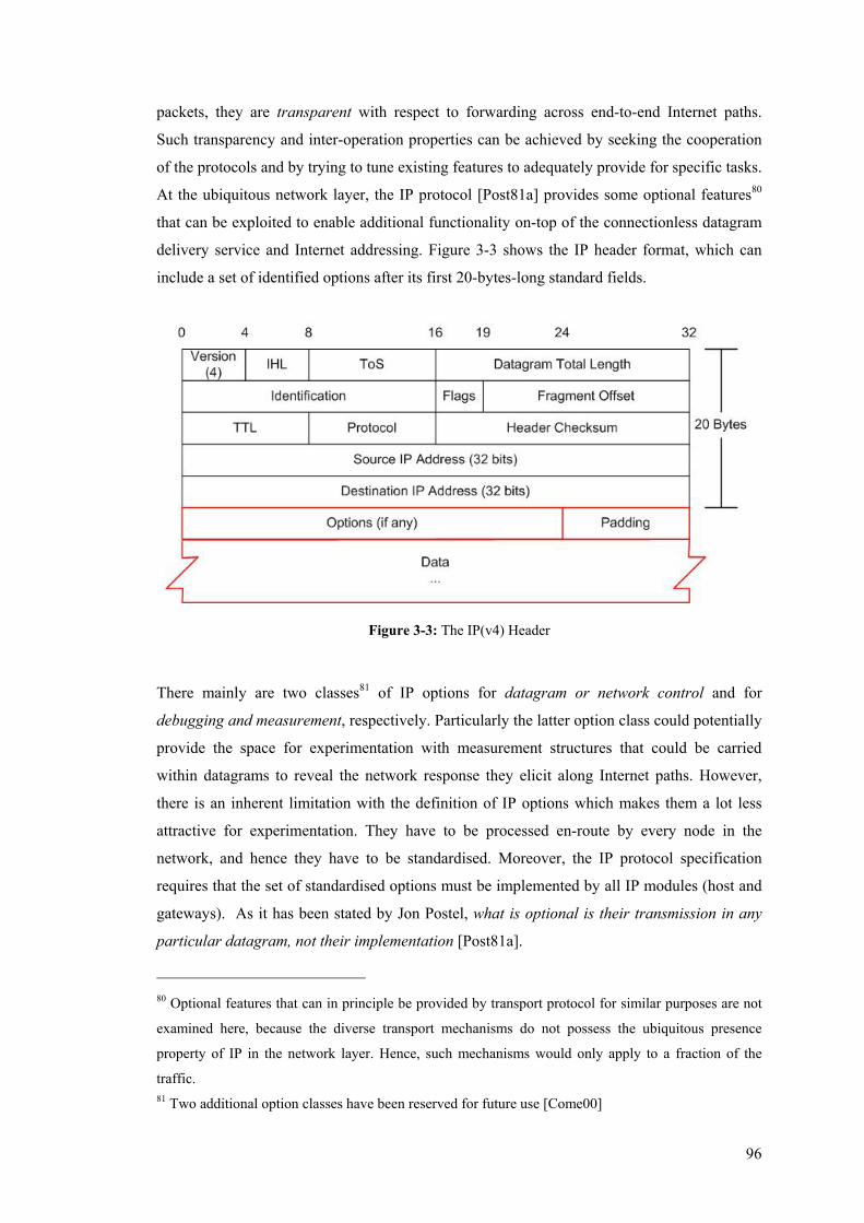
96

packets, they are transparent with respect to forwarding across end-to-end Internet paths.

Such transparency and inter-operation properties can be achieved by seeking the cooperation

of the protocols and by trying to tune existing features to adequately provide for specific tasks.

At the ubiquitous network layer, the IP protocol [Post81a] provides some optional features80

that can be exploited to enable additional functionality on-top of the connectionless datagram

delivery service and Internet addressing. Figure 3-3 shows the IP header format, which can

include a set of identified options after its first 20-bytes-long standard fields.

Figure 3-3: The IP(v4) Header

There mainly are two classes81 of IP options for datagram or network control and for

debugging and measurement, respectively. Particularly the latter option class could potentially

provide the space for experimentation with measurement structures that could be carried

within datagrams to reveal the network response they elicit along Internet paths. However,

there is an inherent limitation with the definition of IP options which makes them a lot less

attractive for experimentation. They have to be processed en-route by every node in the

network, and hence they have to be standardised. Moreover, the IP protocol specification

requires that the set of standardised options must be implemented by all IP modules (host and

gateways). As it has been stated by Jon Postel, what is optional is their transmission in any

particular datagram, not their implementation [Post81a].

80 Optional features that can in principle be provided by transport protocol for similar purposes are not

examined here, because the diverse transport mechanisms do not possess the ubiquitous presence

property of IP in the network layer. Hence, such mechanisms would only apply to a fraction of the

traffic. 81 Two additional option classes have been reserved for future use [Come00]

97

Under the debugging and measurement option class the timestamp [Post81a], and the

traceroute [Malk93] options have been defined. The latter was defined together with a

synonymous ICMP message type to provide for an improved version of the traceroute

debugging tool that would generate fewer packets and complete in a shorter time. The

timestamp option (Figure 3-4) is more general-purpose and it was defined within the main IP

protocol specification to provide for time-related measurement across the Internet. A brief

description of this option will be given mainly to discuss the infeasibility of exploiting this

and similar mechanisms of the network layer for broader measurement experimentation.

Figure 3-4: The IP Timestamp Option

The timestamp option contains an initially empty list of 64-bit entries, and each router along

the path from source to destination fills one entry, usually consisting of its 32-bit IP address

and a 32-bit integer timestamp giving the time and date at which the router handles the

datagram [Come00]. The format of the option is controlled by the flags field whose value

provides for three different modes of operation:

• 0 - Routers can omit their IP address and use the full 64-bit field to insert a timestamp

• 1 - Routers must precede each timestamp by their own IP address

• 3 - IP addresses are specified by the originator host and a router only inserts a timestamp

if the next IP address in the list matches its own IP address

In principle, this option could be used to measure delay and variations of delay experienced by

different packets between sets of identified Internet nodes. Additionally, the possibility of

further defining options that would encode different indicators to assess other performance

metrics of the operational network traffic should also be feasible. However, the need for all IP

modules to support and process all standardised options, impose great and, as experience has

shown, insurmountable difficulties. The option encoding itself does not facilitate option

processing only at identified, targeted nodes. Hence, an IP datagram carrying optional IP data

needs to be examined by every visited node. In the timestamp option for example, even when

the originator specifies which nodes should insert timestamps in the packet (flags value: 3),

98

there is no way a node can tell whether it should insert a timestamp or not before it actually

processes the option list. This general behaviour means that the presence of IP options triggers

additional processing at every node in the network. This automatically implies that the

definition of additional options (e.g. to measure packet loss) is governed by heavy

standardisation and implementation processes across the Internet, which makes their use for

experimental purposes unsuitable. Another (even more) serious implication is that the

additional processing overhead incurred at each hop along an Internet path makes the use of

even the already standardised options impractical. Per-hop additional processing almost

certainly guarantees that packets carrying options will elicit greater response times than the

rest of the traffic. Indeed, experimentation with the IP timestamp option has shown that

routers put packets carrying options on different processing queues and huge differences have

been reported in the processing time of packets with IP options and packets without [Sant03].

In practice, the requirement of en-route processing cannot be seamlessly supported, since

especially high-volume routers don’t have the processing capacity to do that.

3.6 The Internet Protocol version 6 (IPv6) The major implication resulting from Internet’s transition to a commercially driven

communications environment was the dramatic growth of inter-connected hosts and the

consequential exhaustion of the current Internet Protocol (IPv4) address space. Although there

were a number of the original operational characteristics of IP(v4) requiring re-examination, it

became evident that especially the scale issue should be urgently addressed so that the Internet

can accommodate, not only the increasing number of conventional inter-connected hosts, but

also to anticipate IP connectivity for unconventional devices such as intelligent mobile phones

and Personal Digital Assistants (PDA)s, which started providing the technical capabilities

(and challenges) for joining an IP-based global communication medium. Figure 3-5 shows the

latest Internet Domain Survey (conventional) Host Count, as it has been published by the

Internet Systems Consortium (ISC)82. The numbers presented in the survey are considered to

be fairly good estimates of the minimum size of the Internet83. In addition, the Internet

Protocol’s theoretical address space limit of approximately 4.3 billion hosts (232) is further

reduced by its structural division into different class networks, and as it can be seen from

Figure 3-5, the host growth remains exponential.

82 http://www.isc.org/ 83 Other sources estimated 605 million users in 2003, including hosts and mobile devices

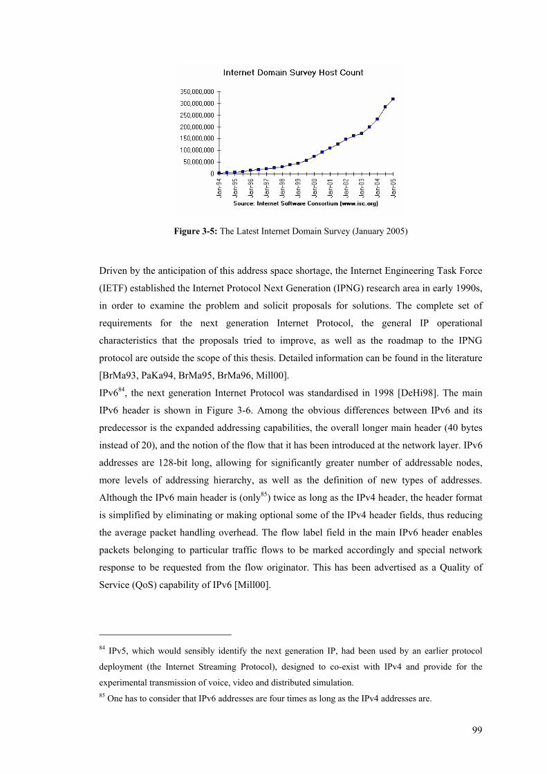
99

Figure 3-5: The Latest Internet Domain Survey (January 2005)

Driven by the anticipation of this address space shortage, the Internet Engineering Task Force

(IETF) established the Internet Protocol Next Generation (IPNG) research area in early 1990s,

in order to examine the problem and solicit proposals for solutions. The complete set of

requirements for the next generation Internet Protocol, the general IP operational

characteristics that the proposals tried to improve, as well as the roadmap to the IPNG

protocol are outside the scope of this thesis. Detailed information can be found in the literature

[BrMa93, PaKa94, BrMa95, BrMa96, Mill00].

IPv684, the next generation Internet Protocol was standardised in 1998 [DeHi98]. The main

IPv6 header is shown in Figure 3-6. Among the obvious differences between IPv6 and its

predecessor is the expanded addressing capabilities, the overall longer main header (40 bytes

instead of 20), and the notion of the flow that it has been introduced at the network layer. IPv6

addresses are 128-bit long, allowing for significantly greater number of addressable nodes,

more levels of addressing hierarchy, as well as the definition of new types of addresses.

Although the IPv6 main header is (only85) twice as long as the IPv4 header, the header format

is simplified by eliminating or making optional some of the IPv4 header fields, thus reducing

the average packet handling overhead. The flow label field in the main IPv6 header enables

packets belonging to particular traffic flows to be marked accordingly and special network

response to be requested from the flow originator. This has been advertised as a Quality of

Service (QoS) capability of IPv6 [Mill00].

84 IPv5, which would sensibly identify the next generation IP, had been used by an earlier protocol

deployment (the Internet Streaming Protocol), designed to co-exist with IPv4 and provide for the

experimental transmission of voice, video and distributed simulation. 85 One has to consider that IPv6 addresses are four times as long as the IPv4 addresses are.

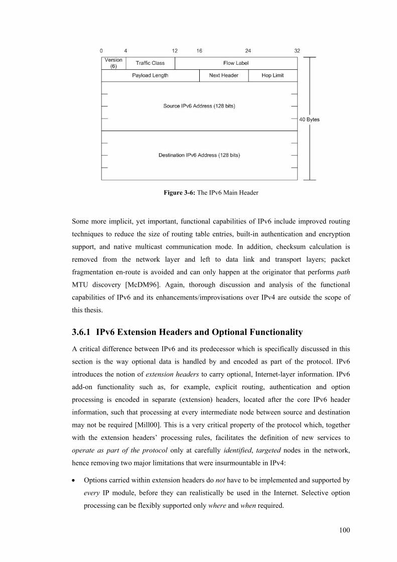
100

Figure 3-6: The IPv6 Main Header

Some more implicit, yet important, functional capabilities of IPv6 include improved routing

techniques to reduce the size of routing table entries, built-in authentication and encryption

support, and native multicast communication mode. In addition, checksum calculation is

removed from the network layer and left to data link and transport layers; packet

fragmentation en-route is avoided and can only happen at the originator that performs path

MTU discovery [McDM96]. Again, thorough discussion and analysis of the functional

capabilities of IPv6 and its enhancements/improvisations over IPv4 are outside the scope of

this thesis.

3.6.1 IPv6 Extension Headers and Optional Functionality

A critical difference between IPv6 and its predecessor which is specifically discussed in this

section is the way optional data is handled by and encoded as part of the protocol. IPv6

introduces the notion of extension headers to carry optional, Internet-layer information. IPv6

add-on functionality such as, for example, explicit routing, authentication and option

processing is encoded in separate (extension) headers, located after the core IPv6 header

information, such that processing at every intermediate node between source and destination

may not be required [Mill00]. This is a very critical property of the protocol which, together

with the extension headers’ processing rules, facilitates the definition of new services to

operate as part of the protocol only at carefully identified, targeted nodes in the network,

hence removing two major limitations that were insurmountable in IPv4:

• Options carried within extension headers do not have to be implemented and supported by

every IP module, before they can realistically be used in the Internet. Selective option

processing can be flexibly supported only where and when required.

101

• The consequential processing overhead from every node having to examine all the options

carried within a datagram is removed. Therefore, option processing can have a minor

impact on the traffic, allowing for options to be carried within the actual data packets

without negatively influencing the network response to these data packets.

IPv6 extension headers are placed between the main IPv6 header and the upper layer header in

a packet. A small number of extension headers have been currently defined, each identified by

a distinct Next Header value. An IPv6 packet can hence carry zero, one, or more extension

headers each identified by the Next Header field of the preceding header, as this is illustrated

in Figure 3-7 [DeHi98].

Figure 3-7: IPv6 Extension Headers’ Encoding

As it is stated in the IPv6 specification, with one exception, extension headers are not

examined or processed by any node along a packet’s delivery path, until the packet reaches

the node identified in the Destination Address field of the IPv6 header. There, normal de-

multiplexing on the Next Header field of the IPv6 header invokes the module to process the

first extension header, or the upper layer header if no extension header is present [DeHi98]. A

full IPv6 implementation includes the implementation of the Hop-by-Hop Options86, Routing

(Type 0), Fragment, Destination Options, Authentication, and Encapsulating Security Payload

extension headers.

When more than one extension headers appear in the same packet, the IPv6 specification

recommends that they are encoded in the following order:

86 This is the only extension header that carries information to be examined and processed by every

node along a packet’s delivery path, including the source and destination nodes.

102

• IPv6 (main) Header

• Hop-by-Hop Options header

• Destination Options header87

• Routing header

• Fragment header

• Authentication header

• Encapsulating Security Payload header

• Destination Options header88

• upper-layer header

According to the IPv6 specification, each extension header should occur at most once in a

datagram, with the exception of the Destination Options header which can occur at most

twice, once before a Routing header and once before the upper-layer header.

A description of the functionality provided by each IPv6 extension header is outside the scope

of this thesis. Interested readers are referred to the appropriate literature resources [DeHi98,

KeAt98a, KeAt98b]. However, the operation of the Routing header will be briefly described

here, in order to emphasise the different attitude adopted by IPv6 regarding additional

functionality and option processing by IP modules. The Routing header89 is used by an IPv6

source to list one or more intermediate nodes to be visited by the packet on its way to the

destination. This functionality is very similar to the IPv4’s Loose Source and Record Route

(LSRR) option [Post81a], but there is a significant difference between how loose source

routing is implemented in IPv6 (by the Type 0 Routing header) and how it is implemented in

IPv4 (by the LSRR option). In IPv6, the originator constructs the list of addresses to be visited

by the packet, and then the address of the first node to be visited is inserted in the Destination

Address field of the main IPv6 header. The rest of the addresses including the ultimate

destination of the packet, are encoded sequentially in the vector of IPv6 addresses within the

Routing header. Hence, the Routing header is not examined or processed until the packet

reaches the node identified in the Destination Address field of the main IPv6 header. In that

87 For options to be processed by the first destination that appears in the IPv6 Destination Address field,

plus subsequent destinations listed in the Routing header 88 For options to be processed only by the ultimate (final) destination of the packet 89 Currently, the Type 0 Routing header has been defined. In the remainder of this thesis, we will refer

to the Routing header, implying the Type 0 Routing header variant.

103

node, the Routing header module is invoked which performs an algorithm to essentially

swap90 the next address to be visited by the packet (as this appears in the Routing header

address vector) with the IPv6 Destination Address. This procedure is repeated until all the

nodes specified in the routing header have been visited, and the ultimate destination address

appears in the Destination Address field of the IPv6 header.

On the contrary, the IPv4 LSRR option contains a fixed vector of addresses to be visited by

the packet, and the ultimate destination appears in the Destination Address field of the IPv4

header from when the packet is first constructed at the originator IP module. Processing the

LSRR option involves every node along the packet’s path having to examine the option fields

and route the packet towards the next IP address appearing in the LSRR address vector.

These different approaches adopted by the two different versions of the Internet Protocol in

order to perform loose source routing, demonstrate the functional capability of IPv6 to invoke

additional processing only at identified nodes in the network, rather than en-route at every

single node. In the Routing header processing example, swapping the IPv6 Destination

Address with the next address in the Routing header’s vector might be a more intensive

operation than simply examining the next address to be visited. However, it only takes place

at pre-identified nodes, rather than at every node along the end-to-end Internet delivery path.

3.6.2 The Destination Options Extension Header

The Destination Options header is used to encapsulate optional information that need to be

examined only by a packet’s ultimate or intermediate destination nodes. It is uniquely

identified by a Next Header value of 60 in the immediately preceding header, and its format is

shown in Figure 3-8.

Figure 3-8: The IPv6 Destination Options Header

The 8-bit Next Header field identifies the type of header immediately following the

Destination Options header, and it uses the same values as the IPv4 Protocol field. The Hdr

Ext Len field contains an unsigned integer that indicates the length of the Destination Options

90 The algorithm also performs error control.

104

header in 8-octet units, not including the first 8 octets. These two fields are followed by a

variable-length Options field which contains one or more Type-Length-Value (TLV)-encoded

options. The requirement for the options is that their length is such that the complete

Destination Options header is an integer multiple of 8 octets long [DeHi98].

Options are only processed by a node whose IPv6 address appears in the Destination Address

field of the main IPv6 header. This would normally be the ultimate destination of a packet, or

in the case of loose source routing, the first destination that appears in the IPv6 Destination

Address field plus subsequent destinations listed in the Routing header91.

Options are currently carried by the Destination Options and the Hop-by-Hop Options headers

and they are encoded in a TLV format, as shown in Figure 3-9.

Figure 3-9: IPv6 TLV-encoded Option format

The Option Type field carries an 8-bit identifier of the type of option, and the Opt Data Len

field contains an unsigned integer indicating the length of the Option Data field of this option,

in octets. The Option Data field is variable-length and it contains Option-Type-specific data.

The Option Type identifiers are internally encoded such that their highest-order two bits

specify the action to be taken by a processing IPv6 node if it does not recognise the Option

Type. The third-highest-order bit of the Option Type specifies whether or not the Option Data

of that option can change en-route to the packet’s ultimate destination [DeHi98]. The

encoding of the different values of the three highest-order bits of the Option Type identifier is

shown in Table 2.

Table 2: Option Type Identifier Internal Encoding

Highest-order two bits

00 Skip over this option and continue processing the header.

01 Discard the packet.

10 Discard the packet and, regardless of whether or not the packet’s Destination

Address was a multicast address, send an ICMP Parameter Problem, Code 2,

message to the packet’s Source Address, pointing to the unrecognised Option

Type

91 These would first be swapped with the IPv6 Destination Address, as it has been described in section

3.6.1.

105

11 Discard the packet and, only if the packet’s Destination Address was not a

multicast address, send an ICMP Parameter Problem, Code 2, message to the

packet’s Source Address, pointing to the unrecognised Option Type

Third-highest-order bit

0 Option Data does not change en-route.

1 Option Data may change en-route.

There currently are only two padding options (Figure 3-10) defined in the IPv6 specification

to be used to pad out an extension header to a multiple of 8 octets in length, and to align

subsequent options when necessary. The Pad1 option is used to insert a single octet of

padding into the Options area of a header. It has a special format, since it does not have a

length and value fields. The PadN option is used to insert two or more octets of padding into

the Options area of a header and its Option Data field consists of the appropriate number of

zero-valued octets.

Figure 3-10: The Two Padding Options Defined for IPv6

The IPv6 specification not only allows but also strongly encourages the definition of new

types of options and extension headers to provide for additional functionality within the

protocol. Optional destination information can be encoded in an IPv6 packet either as options

in the Destination Options header or as separate IPv6 extension headers92. Choosing between

these two approaches can be mainly influenced by factors such as better alignment and

efficient parsing, and also by the desired action of a destination node in case it does not

understand/support the optional information. In this latter respect, the internal option encoding

provides some valuable extensibility and incremental deployment properties that can be

exploited for the definition of new optional functionality to be integrated within IPv6.

92 The Fragment and Authentication headers are two examples of the latter approach.

106

3.7 The Measurement Plane for IPng: A Native

Measurement Technique The extensibility mechanisms of IPv6 discussed in the two previous sections, together with

the incremental design of the Type-Length-Value (TLV)-encoded options provide a sound

basis for embedding and integrating additional functionality within the network layer, which

can operate in parallel with the main forwarding mechanism, without negatively impacting its

performance-critical operation. It is becoming evident that, although the main driving force

for the IPng initiative and the resulting IPv6 specification has been the need to accommodate

the exponentially increasing numbers of addressable nodes, IPv6 itself possesses some strong

explicit and implicit additional capabilities and design enhancements. The extension headers

mechanism in particular, enables additional per-datagram functionality to be encoded in such

a way so that it only impacts specifically identified nodes, and not every intermediate hop

along a packet’s end-to-end Internet path. Essentially, there is an acknowledgement of the

need for add-on services at the Internet layer and IPv6 provides the extension headers

mechanism which moves the required extra processing at the edges of the network, still

maintaining the existing simplicity of datagram forwarding at the core. Although an integral

part of IPv6, extension headers can be considered as residing at an intermediate layer above

network and below transport. Indeed, they possess their own unique IP protocol number as

higher layer protocols do, such as TCP and UDP. From a network node’s perspective,

according to the IPv6 specification, extension headers are treated as higher layer headers

during the forwarding operation. That is, processing of an extension header is separated from

the main IPv6 header processing and takes place based on local rules regarding the Next

Header field of the IPv6 header. A critical difference and advantage of IPv6 over IPv4 is that

options are encapsulated within certain extension headers and not as part of the main IPv6

header. Hence, their presence does not automatically trigger additional processing at every

node, as it was the case with IPv4, and packets carrying options are forwarded identically with

the rest of the traffic, solely based on their main IPv6 header fields. With a single exception93,

options within extension headers are only processed by a node whose IPv6 address appears at

the Destination Address field of the IPv6 header [DeHi98].

Overall, IPv6 has adopted a modular design, and only its basic functionality and processing

rules have been standardised as the core of the next generation Internet Protocol architecture.

Its extensible features can be exploited for experimentation and in order to engineer

93 This exception is the Hop-by-hop Options header. Even in this case though, additional processing at

every node is triggered by the identification of this type of extension header through its protocol

number (IPv6 Next Header field value: 0), and not solely by its presence.

107

additional, native Internet layer mechanisms that can address further requirements as these

become apparent. Early successful exploitation of these features to address inherent

limitations and omissions of today’s Internet design can be not only influential, but also act as

a driving force to urge wide-spread adoption of IPv6 by revealing its benefits and advocating

for its suitability. Along these lines, not standardising a set of options (other than the two

padding options) within the main IPv6 specification might also prove to be a wise decision,

since IPv6 implementations will have to accommodate the space for future optional

definitions, without being tightly coupled to a limited initial set that would inevitably become

the de facto standard, and could prove difficult to extend or change in the future.

In this thesis, the definition of new IPv6 options and their inter-operable encapsulation within

extension headers have been exploited to implement in-line measurements (section 3.4) as a

native performance measurement technique for IPv6 inter-networks. A set of self-contained

TLV-encoded measurement options have been defined to be inserted as part of extension

headers within the actual data packets, and to piggyback measurement indicators along a

datagram’s delivery path. An originator node selects traffic of interest to be instrumented

based on some local policy, and creates the appropriate measurement option to hold the

relevant per-packet measurement indicator, such as a timestamp or a packet counter. The

option is then encoded within an extension header which is inserted between the main IPv6

header and the upper-layer payload. At an identified destination of the packet, the presence of

the specific TLV-encoded (measurement) option within the extension header will trigger a

direct measurement observation, which will in turn implement the corresponding performance

metric to reveal some service quality characteristic of the operational traffic (Figure 3-11).

Figure 3-11: In-Line IPv6 Measurements Operation

108

Processing modules whose invocation will be triggered by the presence of the corresponding

measurement options need be implemented at the identified originator and destination nodes,

to operate in parallel with the IPv6 input and output routines. By residing within the network

layer directly on top of the IPv6 main header, the measurement functionality can be applied to

the wide range of Internet traffic, without being constrained by specific transport or

application-level mechanisms. In-line, IPv6-based measurements are neither totally

independent from the Internet’s forwarding mechanism nor they are limited by infrastructural

and administrative constraints. Rather, they are a measurement mechanism able to instrument

virtually any type of traffic carried on top of IPv6, and are applied directly at the data path by

seeking an affordably minimum level of cooperation and instrumentation only at targeted

network nodes. The measurement mechanism is independent from higher-level measurement

infrastructures and/or processing environments, which can be deployed in a variety of ways to

extract the measurement data and conduct conclusive, large scale and aggregate computations.

By adhering to the standard IPv6 processing rules, in-line measurements can make a

significant contribution to the enforcement of a measurement plane for IPv6 that can

ultimately form an integral part of the next generation Internet architecture. In-line

measurements do not rely on the presence of some dedicated measurement traffic. Instead,

they offer the possibility for any type of operational network traffic to be measured, so that

the real effects of the Internet forwarding mechanism to the different traffic flows can be

revealed, and greater visibility to the network internal behaviour can be given.

3.7.1 Multi-point Measurement

In-line measurements have been designed to operate as a multi-point measurement technique,

where an originator inserts its local measurement indicators in an extension header at the IPv6

layer. These are carried within the packet along an Internet path and are observed, amended

and/or extracted at other instrumented nodes in the network. In its simplest form, in-line

measurement functionality is deployed between two points in the network, a source and a

destination, as shown in Figure 3-11. The reasons for choosing multi-point measurement over

single-point observation are mainly twofold, concerning the capabilities of the measurement

process and the intrusiveness of the aggregate measurement data. As it can be seen at Table 3,

there are three different levels of measurement information that can be targeted by a

measurement approach/system. At the first level, the most primitive type of measurement

information consists of timestamp and counter indicators that can be recorded based on

observations on single data units (packets) as these pass over a single point in the network. By

combining such raw indicators over multiple data units (inter-packet), or at multiple points

(per-packet) in the network, one can compute simple service-oriented performance metrics

such as one-way delay, packet loss and delay variation. Higher-level metrics can be computed

109

based on the statistical and/or temporal properties of simple performance metrics, and can

sometimes be arbitrarily defined, in order to satisfy custom needs of particular measurement

applications94.

Table 3: The Different Levels of Measurement Information

Level Measurement Information Examples

1 Raw, single-point packet measurement indicators Departure/arrival timestamps,

packet counters

2 Simple performance metrics formed by combining raw

measurement indicators One-way delay, packet loss

3 Synthetic, derived metrics formed by the statistical

properties of simple performance metrics

Maximum jitter,

(un)responsiveness/reachability

Measurement architectures that focus on observing raw, single-point per-packet indicators

cannot directly measure the performance experienced by traffic travelling across a network.

Rather, they have to derive/compute simple performance metrics by correlating independent

measurement data from two (or more) points in the network. This is an expensive process that

involves a degree of uncertainty and most importantly cannot be accomplished in a timely

manner. Deriving higher level synthetic metrics is an even more challenging task, and in some

cases might simply be impossible95.

In-line measurements eliminate this need for correlation of measurement data from multiple

observation points, and are able to directly measure the service experienced by traffic between

two (or more) points in the network. Performance metrics can be implemented in real-time by

only combining raw measurement indicators carried within a single data unit, upon reception

of the data unit at a destination node. In addition, in-line measurements can directly target at

specific services, since it is the presence of certain options in the extension header of a packet

that triggers the measurement operation at a destination node. At the same time it is

guaranteed that the same packet has been observed at all the measurement points in the

94 For example, within the PingER project (section 2.2.3), the metric of unreachability is defined to

indicate the event of a remote node not being able to reply in a sequence of 10 probe (ICMP) packets. 95 For example, deriving the maximum jitter for a given flow of traffic by correlating traces from two

passive monitoring probes at the edges of an ISP backbone might not be possible: there is no way to

guarantee that the two monitoring sites observed all the packets of the flow; packets entering at the

same ingress point might have been routed differently and exited at different egress points. In addition,

guaranteeing that both points triggered on the same packet is a very costly operation involving

correlation of large amounts of data, which might simply be infeasible.

110

network. If aggregate measurement data need be exported to some external measurement

system, then performance metrics’ values can be shipped from one (destination) point in the

network, greatly reducing the amount of additional load in the network.

An originator node can choose a fraction of the network traffic to be measured based on some

filtering parameters, and can instrument the data packets with measurement indicators. At a

destination, performance metrics can be implemented directly by observing or amending the

previously inserted measurement indicators. Higher-level performance metrics can also be

derived from the direct measurement of two-point service-oriented metrics.

3.7.2 Ubiquitous Applicability

In-line measurements are applied at the network layer and implicitly exploit its ubiquitous

presence on the next generation Internet. This is a very important property that makes the

technique virtually applicable to the diverse range of Internet traffic, and enables a single

mechanism to assess the service quality characteristics of numerous traffic types. Their

operation directly at the data path constitutes them tuneable to different levels of granularity

and different traffic patterns, by instrumenting operational traffic of interest as this becomes

apparent at selected network nodes. Since they are not dependent on the presence of dedicated

measurement traffic, their periodicity can be configured to measure traffic phenomena of

interest96. In-line measurements can be implemented as small processing modules to operate

in parallel with the IPv6 forwarding engine, and can be deployed incrementally while

maintaining inter-operation with the rest of the Internet infrastructure. Widespread

deployment of the measurement functionality across the IPv6 Internet can be facilitated by the

instantiation of minimal measurement modules at IPv6-capable end-systems97, and can benefit

a large number of different application domains, from end-to-end traffic performance

evaluation, to measurement-based SLA validation and dynamic Traffic Engineering (TE).

3.8 In-Line Measurement Headers and Options A number of indicative in-line IPv6-based measurement entities have been designed as

distinct TLV-encoded options to be encapsulated within the IPv6 Destination Options

extension header (section 3.6.2). Figure 3-12 shows the general format of an IPv6 data packet

carrying a Destination Options extension header which consists of one or more TLV-encoded

measurement options. The figure describes the case where no other extension headers are

present in the packet. The Destination Options extension header is identified by a Next 96 They can, for example, measure a specific traffic flow or all the traffic between two instrumented

nodes for different time intervals. 97 Similar to the ICMP echo responder implementation in today’s networked systems.

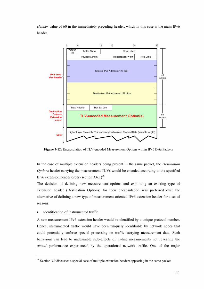
111

Header value of 60 in the immediately preceding header, which in this case is the main IPv6

header.

Figure 3-12: Encapsulation of TLV-encoded Measurement Options within IPv6 Data Packets

In the case of multiple extension headers being present in the same packet, the Destination

Options header carrying the measurement TLVs would be encoded according to the specified

IPv6 extension header order (section 3.6.1)98.

The decision of defining new measurement options and exploiting an existing type of

extension header (Destination Options) for their encapsulation was preferred over the

alternative of defining a new type of measurement-oriented IPv6 extension header for a set of

reasons:

• Identification of instrumented traffic

A new measurement IPv6 extension header would be identified by a unique protocol number.

Hence, instrumented traffic would have been uniquely identifiable by network nodes that

could potentially enforce special processing on traffic carrying measurement data. Such

behaviour can lead to undesirable side-effects of in-line measurements not revealing the

actual performance experienced by the operational network traffic. One of the major

98 Section 3.9 discusses a special case of multiple extension headers appearing in the same packet.

112

requirements for in-line measurements is to circumvent such special response elicitation

which is experienced by some active measurement techniques. Furthermore, the consequences

of instrumented traffic being treated differently than the rest of the traffic can be severe for in-

line measurements, since it is a portion of the actual network traffic and can hence result in

degrading the performance of real applications99. By defining the measurement extensions as

IPv6 TLV-encoded options encapsulated within an existing extension header this concern is

minimised (if not eliminated), since the options are opaque objects for network nodes and

their internals are not revealed simply by observing the Next Header value of the immediately

preceding header. Rather, a network node will attempt to process options contained within an

extension header, only if it is subject to processing this extension header according to the IPv6

specification rules. In our particular scenario of measurement options carried within the

Destination Options100 extension header, only a node whose IPv6 address appears at the

Destination Address field of the main IPv6 header should attempt processing the internals

(options) of the extension header [DeHi98].

• Incremental deployment and inter-operation

In-line measurement functionality should be capable of being incrementally deployed across

the Internet, while maintaining inter-operation with nodes that do not implement measurement

functionality. This is another major requirement since the technique instruments operational

traffic, and it needs to ensure that it does not introduce any disruption to the Internet delivery

service. Experience shows that incremental deployment and backward compatibility is

probably the only way to introduce new services that seek widespread adoption101 to the

Internet architecture.

IPv6 options provide the space for incremental deployment and backward compatibility

through their internal encoding that specifies the action to be taken by a processing IPv6 node,

when it does not recognise the particular Option Type. In contrast, when a destination node

does not recognise the value of an extension header, it should discard the packet and send an

ICMP Parameter Problem message to the source of the packet [DeHi98]. Hence, if in-line

measurements had been defined as a separate extension header, a targeted destination node

that would (for some reason) not implement such functionality would have to discard the

99 This, of course, can also be seen from a slightly different viewpoint: network operators might be

reluctant to treat instrumented traffic differently since the same datagrams also carry application

payload data. 100 In fact, this would be the case for any other extension header except the Hop-by-hop Options header. 101 For example, (widespread) adoption of IPv6 itself is being engineered through transitioning (from

IPv4) and incremental deployment across the Internet.

113

packet and consequently disrupt the service. Using measurement options instead, allows for an

unsupportive node to skip over the option and continue processing the packet’s header(s).

• Semantic redundancy

A desirable characteristic for in-line measurements is to be deployed where and when

required, at identified points in the network. This functionality is provided by the Destination

Options header for IPv6 packets, which facilitates option processing at the ultimate and/or

pre-identified intermediate destinations of a packet (section 3.6.2). Defining a new extension

header to carry measurement data and operate the same way with the existing Destination

Options header could be seen as being semantically redundant for the overall IPv6 operation.

In contrast, the definition of measurement options to be examined at identified destinations

facilitates the exploitation of the appropriate processing mechanisms of the protocol, and

makes good use of its current features. Additionally, it fits well the purpose of a multi-point,

receiver-based measurement technique such as in-line measurements, where measurement

indicators are inserted at an originator, and observed and/or amended at a receiver node.

• Less need for standardisation

From a standardisation perspective, the definition of options is more efficient than the

definition of new extension headers. Of course, option types need to be unique and to be

standardised before options can be widely and unambiguously deployed. However, options

have a narrower, IPv6-internal scope, whereas extension headers, although they refer to the

IPv6 Internet, have a global scope since they need to be uniquely identified within the

protocol stack by a distinct protocol number. Additionally, when new extension headers are

defined, their ordering constraints relative to the existing IPv6 extension headers, as well as

their processing requirements need also be specified and standardised. In contrast, IPv6

options have a pre-specified set of encoding rules and adopt a fixed TLV format which

essentially provides the space to carry option-specific data.

• Efficient parsing and per-packet overhead

Using IPv6 options to design the in-line measurement functionality offers the advantage of

being able to define a set of minimal options to implement different performance metrics.

Different measurements can hence be conducted while incurring a minimal space overhead for

carrying the measurement indicators, and at the same time a minimum processing overhead at

the participating nodes. Simultaneous measurement of different types of metrics using

different options can always be accommodated by encapsulating multiple measurement

options within a single Destination Options header.

On the contrary, if a new extension header had been defined, it would have had to provide the

functionality and space for multiple types of measurement, something that would result in a

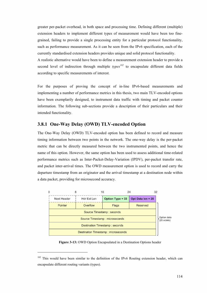
114

greater per-packet overhead, in both space and processing time. Defining different (multiple)

extension headers to implement different types of measurement would have been too fine-

grained, failing to provide a single processing entity for a particular protocol functionality,

such as performance measurement. As it can be seen from the IPv6 specification, each of the

currently standardised extension headers provides unique and solid protocol functionality.

A realistic alternative would have been to define a measurement extension header to provide a

second level of indirection through multiple types102 to encapsulate different data fields

according to specific measurements of interest.

For the purposes of proving the concept of in-line IPv6-based measurements and

implementing a number of performance metrics in this thesis, two main TLV-encoded options

have been exemplarily designed, to instrument data traffic with timing and packet counter

information. The following sub-sections provide a description of their particulars and their

intended functionality.

3.8.1 One-Way Delay (OWD) TLV-encoded Option

The One-Way Delay (OWD) TLV-encoded option has been defined to record and measure

timing information between two points in the network. The one-way delay is the per-packet

metric that can be directly measured between the two instrumented points, and hence the

name of this option. However, the same option has been used to assess additional time-related

performance metrics such as Inter-Packet-Delay-Variation (IPDV), per-packet transfer rate,

and packet inter-arrival times. The OWD measurement option is used to record and carry the

departure timestamp from an originator and the arrival timestamp at a destination node within

a data packet, providing for microsecond accuracy.

Figure 3-13: OWD Option Encapsulated in a Destination Options header

102 This would have been similar to the definition of the IPv6 Routing extension header, which can

encapsulate different routing variants (types).

115

Figure 3-13 shows the internal fields of the TLV-encoded option and their alignment, and also

the encapsulation of the option within a Destination Options IPv6 extension header, by adding

the Next header and Hdr Ext Len fields. Table 4 provides a description of the semantics of the

type, length and value fields for this particular option.

Table 4: OWD Option fields

Type

Option Type 001000012 (33 in decimal)

Length

Opt Data Len 20 Octets (160 bits)

Value

Pointer 8-bit unsigned integer: relative to this option;

smallest legal value for pointer is 7.

Overflow 8-bit unsigned integer: relative to this option

Flags 8-bit unsigned integer: relative to this option

Reserved 8-bit unsigned integer: reserved for future use;

currently set to zero

Source Timestamp: seconds/microseconds 32-bit unsigned integers: timestamp before departure

of packet from the originator

Destination Timestamp: seconds/microseconds 32-bit unsigned integers: timestamp upon reception

of packet at the destination

The Option Type field has been encoded according to the IPv6 specification to indicate the

appropriate action to be taken when a destination node does not understand this option, and

whether option data can change en-route. The decomposition of the binary value of this field

down to three parts (00-1-00001) reveals its internal encoding: the highest-order two bits (00)

specify that if the processing node does not recognise this option, it should skip it over and

continue processing the header and the packet. The third-highest-order bit (1) indicates that

data may change en-route, since the destination of the packet will add its timestamp to the

option. The lowest-order five bits (00001) complete the overall unique Option Type

number103.

103 The lowest-order five bits of the Option Type fields in this section (3.8) have been chosen randomly

(incrementally) for experimentation, without filling a request form at the Internet Assigned Numbers

Authority (IANA). Unfortunately, the IPv6 specification has provided no IANA assignment policy for

experimental code-point values. Hence, different values might need to be chosen for the lowest-order

116

The Opt Data Len field contains the length of the Option Data in octets, and is set to twenty

(20) for the OWD option.

The Option Data fields consist of eight option-type-specific indicators. The Pointer into the

timestamp data is relative to this option and it indicates the octet which begins the next

timestamp to be added. Its minimum legal value is seven (7), pointing at the beginning of the

first timestamp before it is added at the originator of a packet. The Overflow field is used to

indicate if an attempt is made to store more timestamps in the option than there are slots to

accommodate them and it keeps the number of such occurrences. The Flags octet comprises

eight binary flags to store option control information such as the inability of a node to insert a

timestamp for reasons other than overflow, or the nature of data stored elsewhere in the option

data fields. The Reserved field is a zero-valued octet included for future use.

The Source Timestamp is represented by two 32-bit unsigned integers indicating the departure

time of the packet from the interface of the originator, where the option is inserted. The two

integers represent the second and microsecond portions of the time elapsed since 00.00 hours

on 1st January 1970 Universal Coordinated Time (UTC), respectively. Likewise, the

Destination Timestamp is represented by two 32-bit unsigned integers indicating the packet

arrival time at the interface of the node where the extension header option is detected and

processed. It is worth mentioning that the full range of values for some of the 8-bit indicators

of the option has not been unambiguously defined, and they have partly been used for

alignment purposes. Further experimentation with multi-point one-way delay options where

more than two timestamps are accommodated in the Option Data fields can fully exploit these

control octets. For the time being, their existence allows for OWD TLV-encoded option to be

aligned as a single option within a Destination Options header without any padding

requirements, as shown in Figure 3-13.

In contrast to IPv4 being 32-bit aligned, IPv6 is 64-bit aligned so as when 64-bit processors

are used, IPv6 packets are processed much faster than IPv4 packets [Mill00]. Consequently,

each extension header must be an integer multiple of 8 octets (64 bits) long. Under the

assumption [DeHi98] that an option-bearing extension header will carry a minimum number

of options, usually one, the TLV-encoded options in this section (3.8) have been designed so

that they can perfectly align into a single-TLV-carrier Destination Options header as an

integer multiple of 8 octets long, without requiring the insertion of single or multi-octet

padding options. It is visible from Figure 3-13 that a complete destination options header

carrying the OWD option is 24 = 8 x 3 octets (192 bits) long.

five bits of the option types (consequently changing the overall unique Option Type number), if the

options are to be proposed for standardisation.

117

When a Destination Options header carrying an OWD TLV-encoded option is created and

inserted in packet, the originator node records its local timestamp in the option just before the

packet is forwarded to the node’s outgoing interface. Upon reception of the packet at an

incoming interface of a processing node (identified by the Destination Address field of the

main IPv6 header) the presence of the specific option triggers the measurement activity

resulting in the node inserting its local timestamp in the option. Subsequent action regarding

the handling of measurement data as well as further processing of the packet is based on local

polices at the receiving node and the contents of the packet itself.

3.8.2 One-Way Loss (OWL) TLV-encoded Option

The One-Way Loss TLV-encoded option has been defined to record network-level packet

sequence numbers and measure packet loss-related phenomena between two points in the

network. An originator node generates sequence numbers based on some local policy to be

carried within a packet along its delivery path. At an identified destination the sequence

number is observed and stored based on some local policy. By observing sequence numbers of

successive packets that satisfy some common classification criteria, a destination node can

directly measure one-way packet loss occurrences. Figure 3-14 shows the internal fields of the

TLV-encoded option and their alignment, as well as the encapsulation of the option within a

Destination Options IPv6 extension header, by adding the Next header and Hdr Ext Len

fields.

Figure 3-14: One-Way Loss Option Encapsulated in a Destination Options header

The one-way packet loss option has two conceptual differences when compared to the OWD

option (section 3.8.1). First, it has been encoded as a minimal TLV tuple omitting any control

fields in the Option Data area to demonstrate the absolute minimum measurement data

overhead that can be incurred at a packet carrying a Destination Options header. And second,

the one-way loss measurement requires some state to be kept at the instrumented path end-

points, since it is indicators contained in more than one packet that need to be combined in

order to implement this performance metric. Table 5 provides a description of the semantics

of the type, length and value fields for this particular option.

118

Table 5: One-Way Loss Option fields

Type

Option Type 000000112 (3 in decimal)

Length

Opt Data Len 4 Octets (32 bits)

Value

Sequence Number 32-bit unsigned integer: relative to this option;

sequence number inserted at the packet originator

The Option Type has been set to 00-0-00011 (310) to indicate that a processing node that does

not recognise the particular option should skip it over and continue processing the header and

the packet (two highest-order bits – 00), and that the option data may not change en-route

(third-highest-order bit – 0); the destination processing node can only observe and record the

value of the Option Data area.

The Opt Data Len field is set to four (4) for this option, indicating the length of the data area

in octets.

The Option Data consists of a single 32-bit field to hold a network-level packet sequence

number, which is inserted at the packet’s originator node based on some local policy, before

the packet is forwarded to the outgoing interface of the node. As it is shown in Figure 3-14,

the one-way loss TLV-encoded option can be aligned in a Destination Options header without

requiring any padding octets, to construct a single-option 8-octet (64-bit) extension header.

Nodes participating in a one-way loss measurement using the corresponding option need to

accommodate the space and the processing capacity for maintaining state of packet flows for

the duration of the measurement. In contrast to time-related measurements where each packet

can be treated as an individual entity104 between two instrumented points, carrying all the

necessary indicators (timestamps) within its own payload, packet loss measurement requires

packets to be sequenced based on previously sent packets exhibiting some common

characteristic. Flows can be defined at different levels of granularity mainly based on different

header characteristics shared among a group of datagrams; they also have an associated

lifetime threshold after which their activity is considered to be ceased. These issues have been

discussed in section 2.3.2.

Throughout the duration of specific packet loss measurements, instrumented nodes also need

to adhere to the same definition of a flow for the loss indicators to yield meaningful results.

The originator node creates flows and assigns successive sequence numbers to packets 104 Although, in most cases packets are treated as parts of certain flows for time-related measurements

as well; this way metrics can be grouped into and compared between different traffic types.

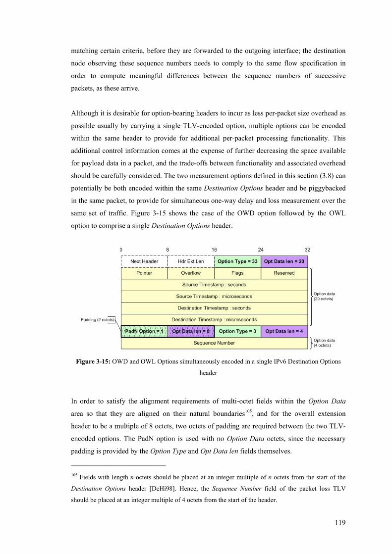
119

matching certain criteria, before they are forwarded to the outgoing interface; the destination

node observing these sequence numbers needs to comply to the same flow specification in

order to compute meaningful differences between the sequence numbers of successive

packets, as these arrive.

Although it is desirable for option-bearing headers to incur as less per-packet size overhead as

possible usually by carrying a single TLV-encoded option, multiple options can be encoded

within the same header to provide for additional per-packet processing functionality. This

additional control information comes at the expense of further decreasing the space available

for payload data in a packet, and the trade-offs between functionality and associated overhead

should be carefully considered. The two measurement options defined in this section (3.8) can

potentially be both encoded within the same Destination Options header and be piggybacked

in the same packet, to provide for simultaneous one-way delay and loss measurement over the

same set of traffic. Figure 3-15 shows the case of the OWD option followed by the OWL

option to comprise a single Destination Options header.

Figure 3-15: OWD and OWL Options simultaneously encoded in a single IPv6 Destination Options

header

In order to satisfy the alignment requirements of multi-octet fields within the Option Data

area so that they are aligned on their natural boundaries105, and for the overall extension

header to be a multiple of 8 octets, two octets of padding are required between the two TLV-

encoded options. The PadN option is used with no Option Data octets, since the necessary

padding is provided by the Option Type and Opt Data len fields themselves.

105 Fields with length n octets should be placed at an integer multiple of n octets from the start of the

Destination Options header [DeHi98]. Hence, the Sequence Number field of the packet loss TLV

should be placed at an integer multiple of 4 octets from the start of the header.

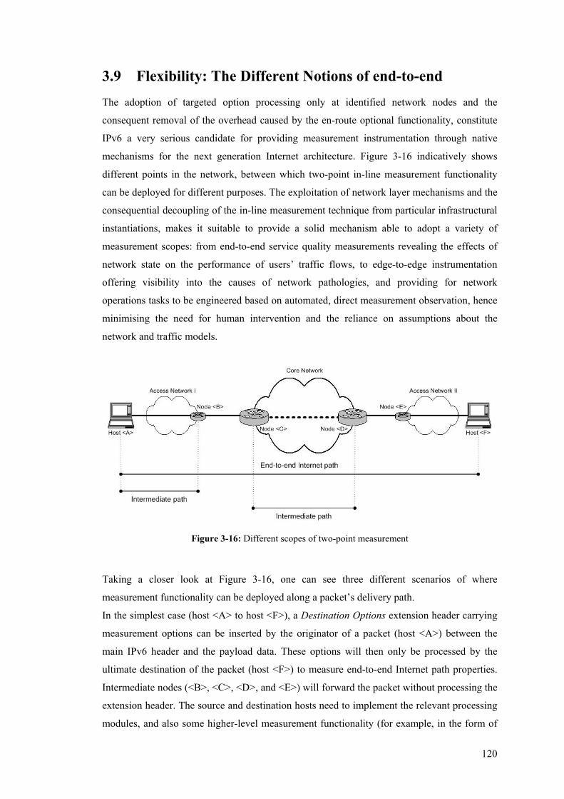
120

3.9 Flexibility: The Different Notions of end-to-end The adoption of targeted option processing only at identified network nodes and the

consequent removal of the overhead caused by the en-route optional functionality, constitute

IPv6 a very serious candidate for providing measurement instrumentation through native

mechanisms for the next generation Internet architecture. Figure 3-16 indicatively shows

different points in the network, between which two-point in-line measurement functionality

can be deployed for different purposes. The exploitation of network layer mechanisms and the

consequential decoupling of the in-line measurement technique from particular infrastructural

instantiations, makes it suitable to provide a solid mechanism able to adopt a variety of

measurement scopes: from end-to-end service quality measurements revealing the effects of

network state on the performance of users’ traffic flows, to edge-to-edge instrumentation

offering visibility into the causes of network pathologies, and providing for network

operations tasks to be engineered based on automated, direct measurement observation, hence

minimising the need for human intervention and the reliance on assumptions about the

network and traffic models.

Figure 3-16: Different scopes of two-point measurement

Taking a closer look at Figure 3-16, one can see three different scenarios of where

measurement functionality can be deployed along a packet’s delivery path.

In the simplest case (host <A> to host <F>), a Destination Options extension header carrying

measurement options can be inserted by the originator of a packet (host <A>) between the

main IPv6 header and the payload data. These options will then only be processed by the

ultimate destination of the packet (host <F>) to measure end-to-end Internet path properties.

Intermediate nodes (, <C>, <D>, and <E>) will forward the packet without processing the

extension header. The source and destination hosts need to implement the relevant processing

modules, and also some higher-level measurement functionality (for example, in the form of

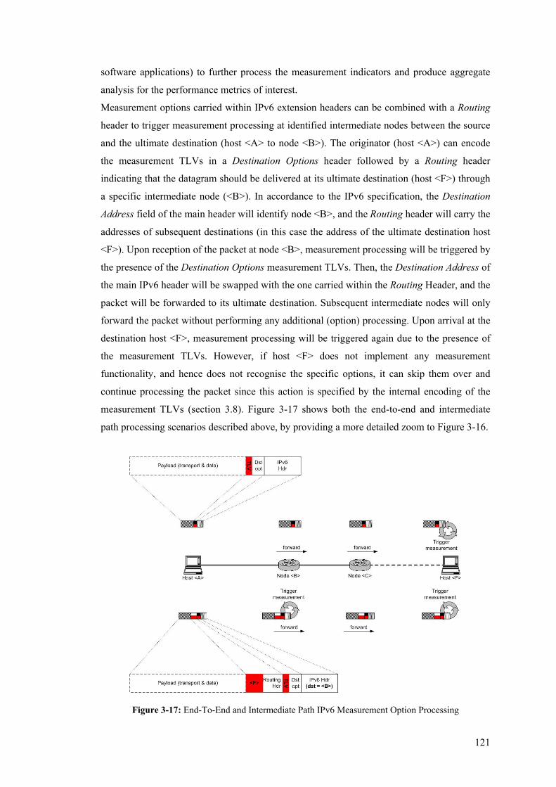
121

software applications) to further process the measurement indicators and produce aggregate

analysis for the performance metrics of interest.

Measurement options carried within IPv6 extension headers can be combined with a Routing

header to trigger measurement processing at identified intermediate nodes between the source

and the ultimate destination (host <A> to node ). The originator (host <A>) can encode

the measurement TLVs in a Destination Options header followed by a Routing header

indicating that the datagram should be delivered at its ultimate destination (host <F>) through

a specific intermediate node (). In accordance to the IPv6 specification, the Destination

Address field of the main header will identify node , and the Routing header will carry the

addresses of subsequent destinations (in this case the address of the ultimate destination host

<F>). Upon reception of the packet at node , measurement processing will be triggered by

the presence of the Destination Options measurement TLVs. Then, the Destination Address of

the main IPv6 header will be swapped with the one carried within the Routing Header, and the

packet will be forwarded to its ultimate destination. Subsequent intermediate nodes will only

forward the packet without performing any additional (option) processing. Upon arrival at the

destination host <F>, measurement processing will be triggered again due to the presence of

the measurement TLVs. However, if host <F> does not implement any measurement

functionality, and hence does not recognise the specific options, it can skip them over and

continue processing the packet since this action is specified by the internal encoding of the

measurement TLVs (section 3.8). Figure 3-17 shows both the end-to-end and intermediate

path processing scenarios described above, by providing a more detailed zoom to Figure 3-16.

Figure 3-17: End-To-End and Intermediate Path IPv6 Measurement Option Processing

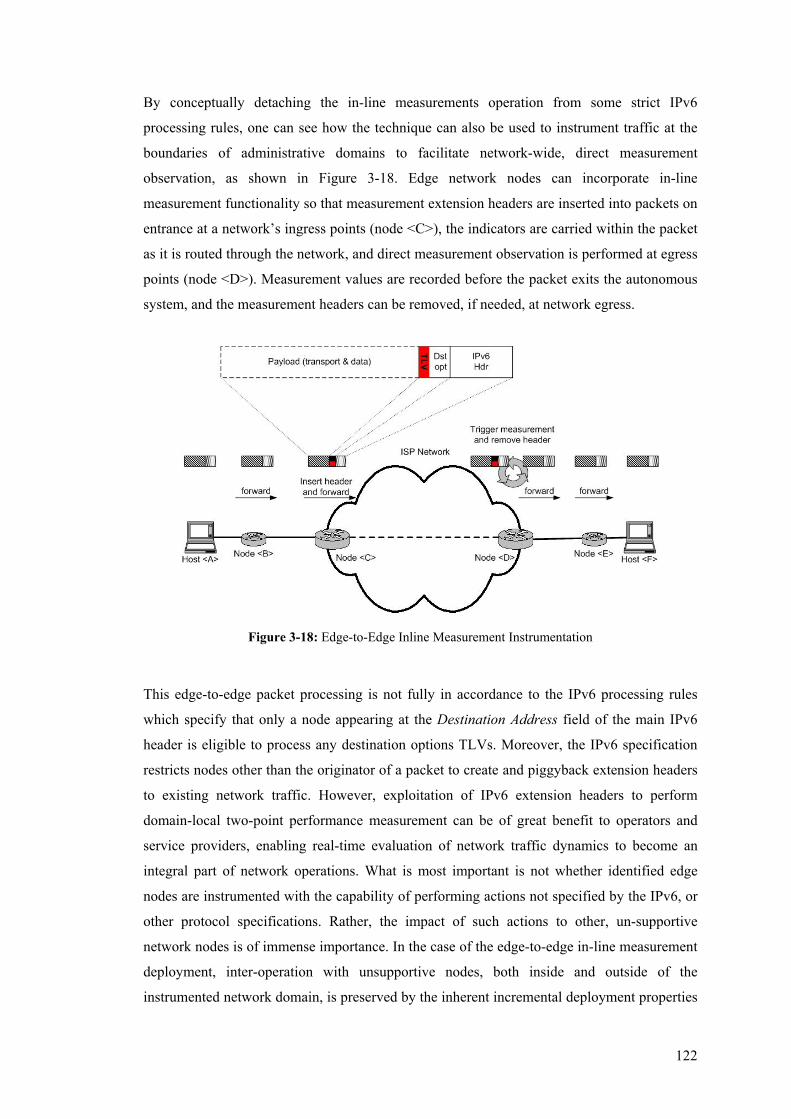
122

By conceptually detaching the in-line measurements operation from some strict IPv6

processing rules, one can see how the technique can also be used to instrument traffic at the

boundaries of administrative domains to facilitate network-wide, direct measurement

observation, as shown in Figure 3-18. Edge network nodes can incorporate in-line

measurement functionality so that measurement extension headers are inserted into packets on

entrance at a network’s ingress points (node <C>), the indicators are carried within the packet

as it is routed through the network, and direct measurement observation is performed at egress

points (node <D>). Measurement values are recorded before the packet exits the autonomous

system, and the measurement headers can be removed, if needed, at network egress.

Figure 3-18: Edge-to-Edge Inline Measurement Instrumentation

This edge-to-edge packet processing is not fully in accordance to the IPv6 processing rules

which specify that only a node appearing at the Destination Address field of the main IPv6

header is eligible to process any destination options TLVs. Moreover, the IPv6 specification

restricts nodes other than the originator of a packet to create and piggyback extension headers

to existing network traffic. However, exploitation of IPv6 extension headers to perform

domain-local two-point performance measurement can be of great benefit to operators and

service providers, enabling real-time evaluation of network traffic dynamics to become an

integral part of network operations. What is most important is not whether identified edge

nodes are instrumented with the capability of performing actions not specified by the IPv6, or

other protocol specifications. Rather, the impact of such actions to other, un-supportive

network nodes is of immense importance. In the case of the edge-to-edge in-line measurement

deployment, inter-operation with unsupportive nodes, both inside and outside of the

instrumented network domain, is preserved by the inherent incremental deployment properties

123

of the technique. The only special requirement for such instantiation is for the instrumented

domain to be able to internally accommodate the marginal increase in the datagram size

caused by the intermediate addition of the measurement headers. Additionally, the egress

edge-nodes where the measurement observation takes place need to remove the measurement

header so that the negotiated end-to-end path MTU is preserved.

By seeking minimal106 cooperation only by nodes at the edges of the network, and by using

existing protocol mechanisms to carry measurement data and act as a trigger to invoke the

measurement activity, the edge-to-edge instantiation of in-line measurement can directly

measure the traffic-perceived performance between domain boundaries. The integration of

such functionality with the IPv6 main forwarding mechanism and the delegation of simple

tasks to operational network nodes can not only complement existing measurement systems,

but in some cases also obviate the need for expensive monitoring and measurement

infrastructures that are independently deployed within ISP networks today.

3.10 Measurement Instrumentation for Next Generation,

all-IP Networks: Applications and Implications In-line measurement is a multi-point, receiver-based technique that can be implemented using

native IPv6 mechanisms between targeted points in the network. A source inserts

measurement indicators into a packet, but it is the receiver that performs a direct observation

on the measurement data carried within the packet. Henceforth, the technique has an intrinsic

unidirectional granularity and bi-directional properties of instrumented paths can be assessed

by combining individual measurements in each path direction. Therefore, it can be used to

among others assess path asymmetries, variable traffic load on different path directions, as

well as different traffic properties between the data and the acknowledgement paths of reliable

transport protocols. Being based on network-level primitives, in-line measurements can

operate either in cooperation with or transparently from the applications, depending on which

points in the network are deployed and what mechanisms of the IPv6 networking stack they

exploit. A major advantage of the technique is that it can be virtually able to instrument any

type of traffic carried over the IPv6 Internet infrastructure. At the same time, the measurement

process is direct, as opposed to post-processing activity on monitored data, and can hence be

targeted to instrument only certain types of traffic, or certain traffic flows, at configurable

levels of granularity.

106 Extension header processing can be seen as a minimal operation which is already included in IPv6

implementations. At the edges of the network, nodes can have the capacity to process IPv6 options, as

well as other more complex admission control and traffic engineering tasks they currently employ.

124

End-to-end in-line measurement can be facilitated by implementing the appropriate processing

modules at end-systems as part of their IPv6 implementation. Measurement data, when

collected at the receiver, can then be fed into either user-space applications or services in

commodity Operating Systems (OS) software that will in turn perform additional processing

and provide users with the performance statistics of their application flows. Such higher-level

software can produce among others visualisations of the measurement data, comparisons

between the performance characteristics of different traffic types and between different

performance metrics of similar traffic types, as well as temporal analysis of (aggregate) traffic

behaviour. Data collected by the measurement modules can also be communicated through

Application Programming Interfaces (API) to common user-space networked applications,

which can in turn implement additional modules to assess the performance of their traffic

flows. In traditional client-server applications such functionality can be used, for example, by

clients to choose appropriate mirrors/caches to receive their content from, based on the actual

properties of their transfers; in more hybrid systems such as peer-to-peer, the participating

entities can use performance measurements to optimise their application-specific inter-

connections and meshes.

At an access network level, in-line measurement functionality can be deployed between end-

systems and the peering nodes of their service provider to evaluate the internal performance of

the network and its effects to user traffic107. Based on such measurement information, and

since this will reflect the properties of the actual traffic, non-flat-rate accounting and billing

schemes can be evaluated, as well as the efficacy of possible traffic differentiation deployed

within the network.

Intermediate path, edge-to-edge in-line measurements between ingress and egress pairs at

domain boundaries can be deployed as additional processing modules at the network edge

nodes. It is not expected that such nodes will run higher-level measurement processing

environments. Rather, they will incorporate the measurement extension header processing

using software and/or hardware support, and they will record the measurement indicators

before shipping them to a measurement data collection point in the network, which can then

perform further, network-wide analysis and operations actions. This can be a Network

Operations Centre (NOC) or some dedicated measurement server. A big advantage of in-line

measurements over existing (passive) techniques concerning this process of measurement data

107 The purpose of such deployment is to essentially measure the “first-hop” performance of the

network traffic. This will not necessarily reflect the end-to-end performance, as this will be influenced

by the network dynamics at the different hops along the traffic’s delivery path. However, performance

measurements at the access network can evaluate how traffic behaviour can be improved by local

policy enforcement controlled by the access provider.

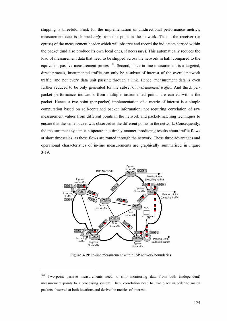
125

shipping is threefold. First, for the implementation of unidirectional performance metrics,

measurement data is shipped only from one point in the network. That is the receiver (or

egress) of the measurement header which will observe and record the indicators carried within

the packet (and also produce its own local ones, if necessary). This automatically reduces the

load of measurement data that need to be shipped across the network in half, compared to the

equivalent passive measurement process108. Second, since in-line measurement is a targeted,

direct process, instrumented traffic can only be a subset of interest of the overall network

traffic, and not every data unit passing through a link. Hence, measurement data is even

further reduced to be only generated for the subset of instrumented traffic. And third, per-

packet performance indicators from multiple instrumented points are carried within the

packet. Hence, a two-point (per-packet) implementation of a metric of interest is a simple

computation based on self-contained packet information, not requiring correlation of raw

measurement values from different points in the network and packet-matching techniques to

ensure that the same packet was observed at the different points in the network. Consequently,

the measurement system can operate in a timely manner, producing results about traffic flows

at short timescales, as these flows are routed through the network. These three advantages and

operational characteristics of in-line measurements are graphically summarised in Figure

3-19.

Figure 3-19: In-line measurement within ISP network boundaries

108 Two-point passive measurements need to ship monitoring data from both (independent)

measurement points to a processing system. Then, correlation need to take place in order to match

packets observed at both locations and derive the metrics of interest.

126

In-line measurements only seek cooperation from nodes at the edges of the network, where

processing capacity can be used to engineer network operations, without impacting the core

nodes which need to perform high-throughput forwarding of aggregate traffic. Appropriate

filtering and sampling schemes can enable in-line measurements to instrument statistically

representative portions of the network traffic and potentially constitute an always-on

mechanism able to continuously measure (and accurately estimate) the performance of

different paths between ingress and egress points, with respect to the temporal traffic

dynamics of the network. A further important property of the technique is that the

measurement activity at a receiver is triggered by the presence of the appropriate header. In

other words, it ensures that a packet carrying a measurement option encoded in an extension

header will be processed by the appropriate module at the receiver which will amend the

measurement option data, if necessary. This behaviour can obviate the need for deploying

network-wide sampling mechanisms (such as, for example, trajectory sampling described in

section 2.3.5.1), to ensure that a packet, if sampled at one point will also be sampled at all

observation points. If, according to some sampling mechanism, a packet is selected to be

instrumented, then the same packet will be observed at the other end of the instrumented sub-

path, due to the presence of the specific options in its extension headers. This property can

even be exploited beyond the pure measurement perspective to provide for edge-to-edge

network control and traffic engineering functionality. According to the types of indicators

defined to be carried within a packet in such a scenario, operations similar in principle to

Multi-Protocol Label Switching (MPLS) [RoVC01] can be defined without the need to

introduce an additional domain-local layer in the networking stack. Extension headers can

potentially be used to carry identifiers based on some characteristic of specific traffic flows, to

provide for differentiated routing and shaping of traffic within an administrative network

domain.

3.11 Summary The injection of additional network load, the periodic and/or on-demand operation, and the

performance assessment of synthetic (not the operational) traffic are the main limitations of

active measurement techniques. Passive monitoring and measurement, on the other hand,

although they can potentially produce accurate results reflecting the actual traffic’s perceived

performance, they mainly suffer from the vast amounts of data that need to be processed, and

the implicit requirement for infrastructural access, that usually limits their scope to single

network and/or administrative domain boundaries. In addition, their single-point passive

operation constitutes the implementation of certain per-packet, service-oriented performance

metrics prohibitively expensive, especially in short timescales.

127

This chapter introduced in-line measurement; a new, multi-point, receiver-based technique

that inserts measurement indicators within the operational traffic units (datagrams) at certain

network nodes, and observes/amends these indicators elsewhere, performing a direct service-

oriented measurement. It can henceforth assess the actual performance experienced by the

traffic between two (or more) points in the (inter-)network. In-line measurement exploits

native mechanisms of the next generation Internet Protocol (IPv6) to insert measurement-

related options at the ubiquitous Internet layer (following the main network-layer header) and

can henceforth measure the performance of virtually any type of traffic carried on top of IPv6.

The design details of the technique and its coupling with IPv6 have been thoroughly

discussed, together with its main advantages of only incurring a marginal processing overhead

to carefully selected network nodes, and not producing dedicated measurement traffic that

could potentially elicit special network response. Additionally, its ability to provide the

ground of a measurement plane for the next generation Internet that can operate in parallel

with the network’s forwarding mechanism and implement numerous performance metrics, its

transparent and seamless inter-operation with un-supportive nodes, as well as its incremental

deployment properties have all been discussed and elaborated. Finally, the feasibility of the

technique to provide for end-to-end, as well as intermediate edge-to-edge performance

measurements, and the beneficial implications of its graceful integration with the IPv6

operation, have also been discussed.

128

Chapter 4

4Implementing In-Line

Measurement in Systems’

Protocol Stacks 4.1 Overview This chapter presents the implementation details of a prototype system to perform in-line

IPv6-based measurements between two points in the network, while adhering to the design

principles described in the previous chapter and consequently demonstrating the main

advantages of the in-line measurement technique. The two-point direct measurement process

consists of the addition of the appropriate IPv6 extension header options at a source, and a

direct measurement observation based on the values carried within these headers at the

destination of an instrumented path. Throughout this chapter, source and destination refer to

the appropriately-instrumented systems that implicitly mark the beginning and the end of an

in-line measurement-capable path, respectively. The instrumented systems may (or may not)

be the ultimate source and destination of a unidirectional measured traffic flow, in which case

in-line measurement is implemented over an end-to-end Internet path.

The prototype system adopts a modular approach that lends itself well to a distributed

measurement framework, where the core measurement components (modules) can

conveniently be added where and when required, hence optimising resource usage and

reducing the associated operational overhead. Different alternatives for the realisation of an

in-line measurement system are discussed, depending on the scope and nature of particular

instantiations of a measurement system, and then a software-based implementation on Linux

129

systems is presented. The realisation of the core in-line measurement components as Linux

dynamically Loadable Kernel Modules (LKM)s is discussed, and the distinctive operations

between modules residing at the source and at the destination of an instrumented path are

highlighted. The different measurement-related actions assumed by LKMs that implement the

One-Way Delay (OWD) and the One-Way Loss (OWL) in-line measurement respectively are

also raised. The mechanisms deployed to facilitate a configurable level of measurement scope

and granularity, and reduce the cost of the measurement process are presented, and a brief

description of the user-space processes that complement the core measurement components of

the prototype concludes this chapter.

4.2 Decouple the Measurement Technique from Particular

Measurement Applications One of the main purposes of the in-line measurement prototype implementation is to

demonstrate the suitability of the proposed measurement technique for a variety of operational

and organisational scenarios. Additionally, the implementation should reflect the potentially

ubiquitous applicability of the measurement technique to all-IPv6 networks and traffic flows,

as well as its inter-operation with existing system software and applications.

The mechanism for direct measurement observation of packet-level indicators exploiting

native IPv6 features can be independent from measurement applications and higher-level

measurement paradigms, which can in turn implement a variety of performance metrics based

on the indicators carried within the instrumented traffic.

An alternative, integrated implementation that would couple the in-line measurement

operation with particular higher-level instrumentation applications can essentially instantiate

an active-measurement-like multi-point infrastructure where remote systems act as beacon

servers [CoLW03, GeGK01], sending and/or receiving instrumented traffic to measure the

performance characteristics of their interconnecting Internet paths. Such a system could

potentially be realised as a set of applications109 (possibly) able to exchange multiple types of

IPv6 traffic, encode in-line measurement data as TLV options, and then exploit the functions

provided by the advanced sockets API for IPv6 [StTh98] to encapsulate individual

(measurement) options within IPv6 Destination Options header structures to be piggybacked

to the generated traffic. At a receiving node, the application can process and decode the

measurement options carried within the destination options header of a packet, simply by

109 Such applications can have equivalent functionality to traffic generators.

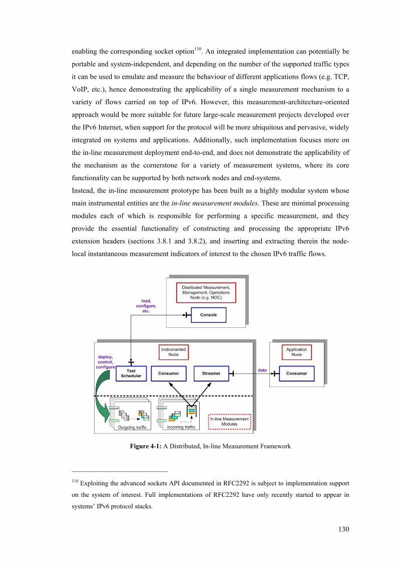
130

enabling the corresponding socket option110. An integrated implementation can potentially be

portable and system-independent, and depending on the number of the supported traffic types

it can be used to emulate and measure the behaviour of different applications flows (e.g. TCP,

VoIP, etc.), hence demonstrating the applicability of a single measurement mechanism to a

variety of flows carried on top of IPv6. However, this measurement-architecture-oriented

approach would be more suitable for future large-scale measurement projects developed over

the IPv6 Internet, when support for the protocol will be more ubiquitous and pervasive, widely

integrated on systems and applications. Additionally, such implementation focuses more on

the in-line measurement deployment end-to-end, and does not demonstrate the applicability of

the mechanism as the cornerstone for a variety of measurement systems, where its core

functionality can be supported by both network nodes and end-systems.

Instead, the in-line measurement prototype has been built as a highly modular system whose

main instrumental entities are the in-line measurement modules. These are minimal processing

modules each of which is responsible for performing a specific measurement, and they

provide the essential functionality of constructing and processing the appropriate IPv6

extension headers (sections 3.8.1 and 3.8.2), and inserting and extracting therein the node-

local instantaneous measurement indicators of interest to the chosen IPv6 traffic flows.

Figure 4-1: A Distributed, In-line Measurement Framework

110 Exploiting the advanced sockets API documented in RFC2292 is subject to implementation support

on the system of interest. Full implementations of RFC2292 have only recently started to appear in

systems’ IPv6 protocol stacks.

131

As it will become evident in later sections, different modules operate on incoming and

outgoing IPv6 traffic at an instrumented node, performing distinctive tasks depending on

whether traffic to be instrumented leaves the system111, or already instrumented traffic enters

the system. Figure 4-1 shows these different operations of the in-line measurement modules

and most importantly their role in a distributed measurement framework environment.

An instrumented node is an abstraction of an IPv6 network entity (a router or an end-system)

that deploys one or more measurement modules to either instrument IPv6 traffic by

piggybacking in-line measurement data within IPv6 Destination Options headers, or to

conduct a direct measurement observation112 to already instrumented traffic as it enters the

node. The measurement modules can be initialised and terminated by a test scheduler process

which can control their operation and configure their parameters, specifying, for example,

which types of traffic are to be instrumented or how to export the collected measurement

indicators to other, higher-level processes. The test scheduler can operate locally at an

instrumented node providing the interface between an operator and the in-line measurement

modules, or it can be remotely controlled by a node conceptually equivalent to a network

management station, which would control the in-line measurement operation on a set of

instrumented nodes within a network domain. Measurement data produced by the observation

and/or amendment of indicators carried in the relevant IPv6 destination header options of

incoming traffic is exported by the corresponding module as input to consumer processes

responsible for further tasks, which can vary from measurement analysis, visualisation and

aggregation, to complex measurement-based traffic policing and control. As with the test

schedulers, consumers can also reside either on the instrumented node or on a remote system,

depending on the overall framework of measurement operation. In case the instrumented node

is an end-system that has the processing capacity to deploy higher-level analysis processes,

consumers can run locally to assess and visualise the performance of application flows113. In a

network-wide distributed measurement scenario where instrumented nodes are edge routers, it 111 Either originates at the instrumented node or it is further forwarded. 112 The term direct measurement observation is highlighted in order to emphasise that the appropriate

modules perform a direct measurement on incoming, already instrumented traffic, by amending and/or

calculating specific metrics of interest based on indicators carried in the measurement extension header

options. This process is fundamentally different from passive monitoring, where traffic is monitored

based on some local pre-configuration decision. In contrast to passive monitoring where the

measurement of specific metrics is a post-processing task, in-line measurements make a direct

observation (measurement) of a specific metric, and it is the analysis and/or further interpretation of the

measurement data which is left for post-processing. 113 This scenario assumes that the remote system(s) will also implement some measurement modules to

at least instrument traffic sent to the end-system of interest.

132

would be expected that they only deploy the minimal measurement modules to provide the

edge-to-edge traffic instrumentation. Measurement data can then be streamed to remote

dedicated systems which would in-turn locally instantiate consumers to deal with among

others the higher-level processing, visualisation and/or archival of data.

Figure 4-1 essentially reveals two different levels of operation of an in-line measurement

framework, by using loosely-coupled components to implement a set of well-identified tasks

and to stress the benefits of a modular approach, which only places the additional processing

intelligence where and when required. The design details discussed in this section provide an

additional level of detail to the applications and implications of the in-line measurement

technique raised in section 3.10. The great potential of the technique is stressed by its

seamless integration with the IPv6 functionality which makes its realisation feasible at both an

end-to-end level on end-systems, and at a network-wide edge-to-edge level on boundary

routers. In the simpler case, in-line measurement functionality can be incrementally built for

end-systems as a set of operating system modules that can provide measurement feedback for

end-users. The instrumented nodes in this case are end-systems which implement the

measurement modules as well as the higher-level processing and configuration components,

such as test schedulers and consumers114. In the more complex case of a two-point edge-to-

edge measurement over a network domain, the instrumented edge nodes can implement the

minimal functionality of the measurement extension header processing, and operations such as

measurement scheduling and analysis can be performed remotely under a network-wide

measurement framework115. The overall implementation details of such a distributed

measurement framework and the inter-dependencies between its different components are

outside the scope of this thesis. The remainder of the chapter will focus on the prototype

implementation of the in-line measurement modules and some example higher-level

processing applications.

114 Comparable functionality can be found in today’s operating systems that implement packet

scheduling and bandwidth reservation modules for QoS-aware applications. 115 Additional measurement processing locally at the network nodes is also possible; however, its

impact on the forwarding performance of the node will have to be carefully examined.

133

4.3 Measurement Instrumentation within Network Nodes

and End-Systems Depending on the purpose and scope of a particular implementation of the in-line

measurement technique, the instrumentation can be realised in a variety of ways.

The measurement modules which are the basic components employed in the prototype need to

provide the time-critical, real-time operation of instrumenting nodes to facilitate in-line

measurement techniques through the addition, modification and possibly removal of data in

the extension headers.

At a system level the main required functionality for performing in-line measurements such as

one-way delay and loss can be implemented, for example, by using dynamically loadable

modules to provide additional processing logic for the manipulation of options in packet

headers and other supporting functions such as the storage, retrieval and forwarding of

measurement-related data. By modularising the set of monitoring and measurement tasks it is

possible to dynamically load only those modules that are needed at a particular time and then

unload them once they are no longer required. The loadable in-line measurements modules

may be remotely delivered to the nodes, loaded and configured and, whilst in use, effectively

become an integral, embedded part of the nodes’ operating software.

Especially when in-line measurements are targeted at forming the core of an intelligent

network Operational Support System (OSS) by implementing the additional functionality on

edge network nodes, minimisation of the actively used processing logic by modularisation can

reduce memory usage, speed up processing time, limit circuit-board space requirements,

simplify designs and reduce overall subsystem complexity. This modular approach also lends

itself well to a remote, distributed implementation since the modules can be freely inserted

and removed around the network as required, providing a potential for dynamically-

configurable, localised processing sites and correlation entities. Another significant advantage

of the embedded module approach is that it is not necessary to physically connect into the

electrical or optical cables comprising the links between routers in order to monitor passing

data, as it is the case for hardware-assisted passive monitoring probes. The embedded module

approach instead makes use of spare programmable logic or processing capability within the

network devices, providing a more integrated, inherently powerful solution. Upgrades can also

be accounted for by delivering new modules to nodes (for example over the network itself),

which can either be directly loaded on delivery or be temporarily stored on some form of local

media (e.g. hard disc storage) for later use.

Figure 4-2 shows an illustrative architecture of a single network element with a number of line

interfaces and a controller comprising a processor, memory and program software or

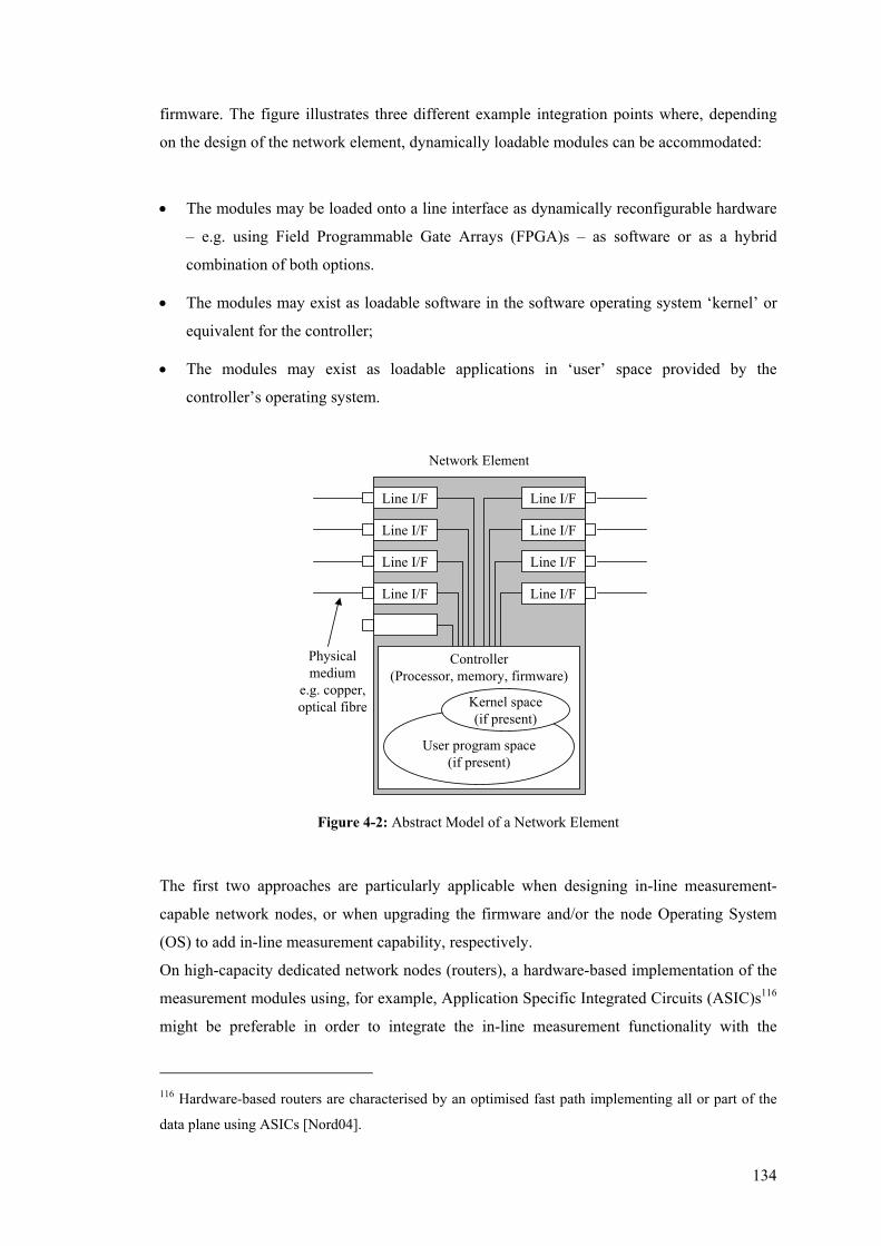
134

firmware. The figure illustrates three different example integration points where, depending

on the design of the network element, dynamically loadable modules can be accommodated:

• The modules may be loaded onto a line interface as dynamically reconfigurable hardware

– e.g. using Field Programmable Gate Arrays (FPGA)s – as software or as a hybrid

combination of both options.

• The modules may exist as loadable software in the software operating system ‘kernel’ or

equivalent for the controller;

• The modules may exist as loadable applications in ‘user’ space provided by the

controller’s operating system.

Line I/F

Line I/F

Line I/F

Line I/F

Line I/F

Line I/F

Line I/F

Line I/F

Network Element

Physicalmedium

e.g. copper,optical fibre

Controller(Processor, memory, firmware)

User program space(if present)

Kernel space(if present)

Figure 4-2: Abstract Model of a Network Element

The first two approaches are particularly applicable when designing in-line measurement-

capable network nodes, or when upgrading the firmware and/or the node Operating System

(OS) to add in-line measurement capability, respectively.

On high-capacity dedicated network nodes (routers), a hardware-based implementation of the

measurement modules using, for example, Application Specific Integrated Circuits (ASIC)s116

might be preferable in order to integrate the in-line measurement functionality with the

116 Hardware-based routers are characterised by an optimised fast path implementing all or part of the

data plane using ASICs [Nord04].

135

router’s fast path. Not using dedicated hardware would result in the measurement

instrumentation to be handled by the control processor, which offers significantly lower

throughput (slow path), and consequently, an increased number of instrumented flows would

negatively impact the router’s processing capacity. However, ASIC-based solutions are not

programmable. Network Processors (NP)s are another emerging technology for high-speed

packet forwarding and manipulation that offers the advantage of programmability over ASICs,

and could potentially be exploited as an alternative to implement the measurement module

functionality at high line speeds. NP design is an area attracting much attention at the

moment, but is still at its early stages, not fully inline with increases in network transmission

technologies117. Also, programming a NP involves the challenges of fully utilising the

available memory bandwidth to sustain the maximum required packet rate and to allow the NP

to be programmed more dynamically without violating its timing constraints [SpKP01].

Further discussion of the alternative hardware-assisted implementations for the in-line

measurement modules to support certain line rates and/or be integrated to specific router

implementations is outside the scope of this thesis. However, it is envisaged that optimised

implementations for dedicated systems can be achieved, similar to today’s hardware-based

MPLS implementations and IPv4/IPv6 features incorporated in certain networking products

and platforms [Rive00, Cisc05].

Integrating measurement modules as part of a node’s Operating System (OS) ‘kernel’ and/or

‘user space’ is a more suitable approach for implementing the additional functionality on

software-based routers and end-systems running on commodity hardware PC configurations.

Although the performance of a software-based system will inevitably be less optimal than

hardware-accelerated solutions, it serves well the purposes of the prototype which aims at

demonstrating the applicability of the technique and its inter-operation with general principles

of system software, rather than its suitability for particular hardware and software

configurations. Additionally, if the in-line measurement functionality is included within end-

systems IPv6 stacks’ implementations, then a software-based solution is more likely to be

seen even in production environments, since the cost of high-end customised hardware

components might be too high to be accounted for at general-purpose PC configurations.

Integration of measurement modules as loadable kernel software assumes a suitably-compliant

Operating System (OS) such as, for example, Linux®, which allows to dynamically load and

unload components of the operating system (kernel) through the Loadable Kernel Modules

(LKM)s mechanism [Rusl99, Hend05]. These typically provide better processing

performance compared to applications executing in user space, and can easily be configured to

117 For example, NP technology was able to support line speeds approaching OC-48 in 2001, but the

already available OC-192 line rates were outside the reach of existing products [SpKP01].

136

add, remove and modify extension headers as an integral part of the kernel’s implementation

of the network protocol stack rather than having to explicitly construct entire packets in an

external user-space process.

Processing IPv6 extension headers in user space, rather than as part of the operating system’s

protocol stack implementation, may not be as elegant a solution and may result in poorer

performance. However, it does not require knowledge of operating system kernel

programming techniques and therefore may be simpler to implement. In addition it avoids

possible problems with operating system security and integrity which may conflict with

security policies of an organisation operating the routers or other nodes in question.

4.4 In-Line Measurement Technique: The Prototype The in-line measurement prototype implementation has been realised on the Linux Operating

System (OS), and specifically, on kernel versions 2.4.18 and 2.4.19. Linux supported IPv6

well at the time of development, as it has incorporated the protocol in its main kernel

relatively early, since production series 2.2. The IPv6 implementation in Linux is being

compliant to the basic IPv6 API [GiTB99]. The extended API for IPv6 [StTh98] which

standardises among others the functions and socket options that applications can use to send

and receive IPv6 extension header options is only partly118 implemented. However, this lack

of full-features implementation for IPv6 did not constrain the prototype development in any

way, which only assumed a basic IPv6 stack implementation and packet processing. It would

have been constraining if the prototype assumed support for user applications to create,

encode and send their specific information into IPv6 Destination Options extension headers.

At the same time there were a growing number of user processes, servers and daemons

incorporating IPv6 in the open source community that facilitated experimentation and

evaluation of the prototype against existing systems and IPv6 application traffic flows.

In October 2000, the USAGI [Usag05] project started in Japan to implement missing or

outdated IPv6 support in Linux, but its releases had not been included in the Linux kernel 2.4

series, resulting in the 2.4 series missing some IPv6 extensions119 and not conforming to all

current RFCs. This partial support for IPv6 was similar, if not worse120, to other operating

systems, making Linux favourable due to the large user community involved in continuously

118 Although the 2.2 kernel has near complete support for receiving options, the macros for generating

IPv6 options are missing in glibc 2.1. 119 Even within the USAGI project, partial implementation of RFC2292 started appearing in early 2002

[Kand02] 120 For example, the official Microsoft® line was that the IPv6 options are not supported on Windows

2000 [Faq605].

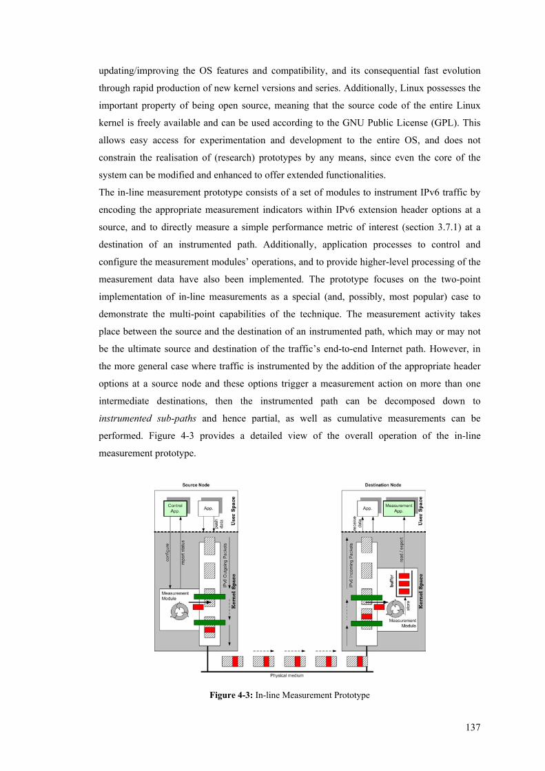
137

updating/improving the OS features and compatibility, and its consequential fast evolution

through rapid production of new kernel versions and series. Additionally, Linux possesses the

important property of being open source, meaning that the source code of the entire Linux

kernel is freely available and can be used according to the GNU Public License (GPL). This

allows easy access for experimentation and development to the entire OS, and does not

constrain the realisation of (research) prototypes by any means, since even the core of the

system can be modified and enhanced to offer extended functionalities.

The in-line measurement prototype consists of a set of modules to instrument IPv6 traffic by

encoding the appropriate measurement indicators within IPv6 extension header options at a

source, and to directly measure a simple performance metric of interest (section 3.7.1) at a

destination of an instrumented path. Additionally, application processes to control and

configure the measurement modules’ operations, and to provide higher-level processing of the

measurement data have also been implemented. The prototype focuses on the two-point

implementation of in-line measurements as a special (and, possibly, most popular) case to

demonstrate the multi-point capabilities of the technique. The measurement activity takes

place between the source and the destination of an instrumented path, which may or may not

be the ultimate source and destination of the traffic’s end-to-end Internet path. However, in

the more general case where traffic is instrumented by the addition of the appropriate header

options at a source node and these options trigger a measurement action on more than one

intermediate destinations, then the instrumented path can be decomposed down to

instrumented sub-paths and hence partial, as well as cumulative measurements can be

performed. Figure 4-3 provides a detailed view of the overall operation of the in-line

measurement prototype.

Figure 4-3: In-line Measurement Prototype

138

The technique is directly employed on the data path to instrument and measure the actual IPv6

traffic flows that pass by selected network nodes, and hence the prototype is not operating on

some kind of special-purpose measurement traffic, over whose generation rates and

periodicity intervals it could have control. Rather, the measurement modules need to be able

to operate on more aggregate traffic as this appears at an instrumented node, a requirement

that makes their operation time-critical and stresses for an efficient implementation, even for

the purposes of the prototype. Therefore, since performance was of prime concern, the

measurement modules have been wholly implemented in kernel space directly coupled with

the IPv6 protocol stack implementation. The modules essentially extend the functionality of

the protocol stack by being attached to the IPv6 input and output routines, and provide the

ability to the kernel to either instrument selected IPv6 packets with measurement extension

header options before transmitting them over the network, or make a direct measurement

observation based on the presence of the appropriate extension header options upon reception

of IPv6 datagrams.

At the source node of an instrumented path, IPv6 packets are examined by the measurement

module before they are sent over the network interface, and if they satisfy certain selection

criteria they are instrumented. An appropriate IPv6 measurement option is created to carry the

relevant instantaneous raw measurement indicator (section 3.7.1) and the whole option is

encoded within an IPv6 Destination Options header, which is then inserted between the main

IPv6 header and the upper-layer data. Packet handling is then returned to the kernel’s normal

IPv6 output functions and the datagram is eventually sent over the network. Upon reception of

packets at the destination node of an instrumented path, the corresponding measurement

module examines their contents as soon as they are passed to the IPv6 protocol handling

routine. The presence of an IPv6 Destination Options header and the appropriate measurement

option therein trigger the measurement activity by the module, which updates the header’s

measurement fields (if necessary) and then stores the measurement-related packet data in a

First In First Out (FIFO) buffer. The packet is then returned to standard kernel code which

takes on processing through the layers of the protocol stack121.

An alternative user-space implementation of the measurement modules would require

outgoing and incoming IPv6 datagrams to be queued for user-space handling, and then be

returned to the kernel to complete their processing through the remaining layers of the

networking stack. This would result in a considerable replication of state between the kernel-

level IPv6 stack and the user-level measurement modules, seriously impairing the

121 The measurement option or even the entire IPv6 Destination Options header may (Figure 4-3) or

may not be removed from the packet by the measurement module at the destination of an instrumented

path. The different alternatives will be discussed in later sections.

139

performance of the overall system due to large scheduling and memory management issues

involved in moving data and control between kernel-level and user-level address spaces.

Hence, although a kernel-level approach leads to more challenges and difficulties during

development, and constitutes parts of the prototype system-dependent, it significantly

improves the response time of measurement modules and minimises their impact on the

effective throughput of network traffic, since the additional time-critical per-packet processing

takes part solely within the kernel’s implementation of the network (IPv6) stack.

Moreover, the implementation of the measurement modules within the OS kernel guarantees

their complete transparency (and hence seamless inter-operation) to applications. Not only

applications do not have to provide any additional functionality, they do not even need to be

aware of the presence of the measurement options in their traffic flows, since even if the

module at the destination node does not remove the relevant options from the packet, these

would only be delivered to the application if it explicitly asked for them through the

corresponding socket option.

Apart from the measurement modules that are the actual in-line instrumentation entities of the

prototype, user-space processes have also been developed to configure the modules’ operation

and to process the measurement data exported from the module(s) at the destination of an

instrumented path (Figure 4-3). Control applications configure the parameters of the overall

measurement process, such as the length of the measurement period and its on-demand

initiation and termination. Additionally, at the source122 of an instrumented path, the control

application sets the internal parameters of the measurement activity, such as the type of

measurement (to be) employed and the measurement granularity. Higher-level analysis

applications read the measurement data from the buffer of the module at the destination of an

instrumented path in regular intervals. The applications can then derive higher-level synthetic

performance metrics based on further computations on the simple metrics directly

implemented by the modules, and on several packet header values carried within the

instrumented IPv6 traffic. For the purposes of the prototype, the user-space control and

analysis processes have been implemented locally, on the instrumented nodes. This has been

feasible because the experimental machines consisted of Linux software routers and end-

systems on commodity PC configurations that provided the required additional processing

capacity. This setup mainly offers the advantage of measurement data not being shipped over

the network while the modules operate, and not competing with the instrumented traffic,

122 More parameters are externally configured for the measurement modules operating at the source of

an instrumented path to create and insert the appropriate measurement options. At the path’s destination

the main direct measurement activity is automatically triggered by the presence of the relevant IPv6

extension header options.

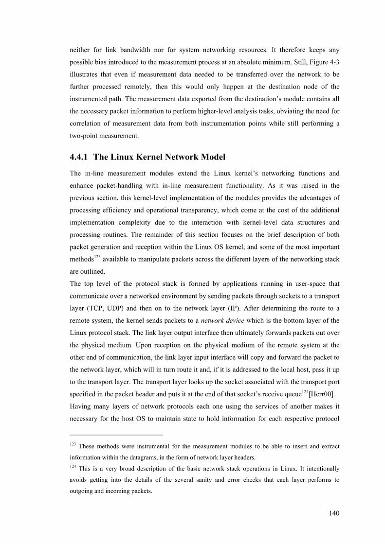
140

neither for link bandwidth nor for system networking resources. It therefore keeps any

possible bias introduced to the measurement process at an absolute minimum. Still, Figure 4-3

illustrates that even if measurement data needed to be transferred over the network to be

further processed remotely, then this would only happen at the destination node of the

instrumented path. The measurement data exported from the destination’s module contains all

the necessary packet information to perform higher-level analysis tasks, obviating the need for

correlation of measurement data from both instrumentation points while still performing a

two-point measurement.

4.4.1 The Linux Kernel Network Model

The in-line measurement modules extend the Linux kernel’s networking functions and

enhance packet-handling with in-line measurement functionality. As it was raised in the

previous section, this kernel-level implementation of the modules provides the advantages of

processing efficiency and operational transparency, which come at the cost of the additional

implementation complexity due to the interaction with kernel-level data structures and

processing routines. The remainder of this section focuses on the brief description of both

packet generation and reception within the Linux OS kernel, and some of the most important

methods123 available to manipulate packets across the different layers of the networking stack

are outlined.

The top level of the protocol stack is formed by applications running in user-space that

communicate over a networked environment by sending packets through sockets to a transport

layer (TCP, UDP) and then on to the network layer (IP). After determining the route to a

remote system, the kernel sends packets to a network device which is the bottom layer of the

Linux protocol stack. The link layer output interface then ultimately forwards packets out over

the physical medium. Upon reception on the physical medium of the remote system at the

other end of communication, the link layer input interface will copy and forward the packet to

the network layer, which will in turn route it and, if it is addressed to the local host, pass it up

to the transport layer. The transport layer looks up the socket associated with the transport port

specified in the packet header and puts it at the end of that socket’s receive queue124[Herr00].

Having many layers of network protocols each one using the services of another makes it

necessary for the host OS to maintain state to hold information for each respective protocol

123 These methods were instrumental for the measurement modules to be able to insert and extract

information within the datagrams, in the form of network layer headers. 124 This is a very broad description of the basic network stack operations in Linux. It intentionally

avoids getting into the details of the several sanity and error checks that each layer performs to

outgoing and incoming packets.

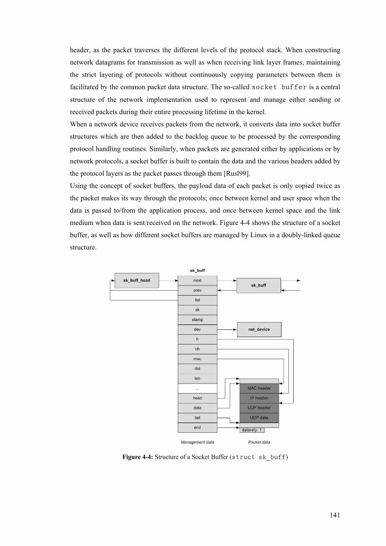
141

header, as the packet traverses the different levels of the protocol stack. When constructing

network datagrams for transmission as well as when receiving link layer frames, maintaining

the strict layering of protocols without continuously copying parameters between them is

facilitated by the common packet data structure. The so-called socket buffer is a central

structure of the network implementation used to represent and manage either sending or

received packets during their entire processing lifetime in the kernel.

When a network device receives packets from the network, it converts data into socket buffer

structures which are then added to the backlog queue to be processed by the corresponding

protocol handling routines. Similarly, when packets are generated either by applications or by

network protocols, a socket buffer is built to contain the data and the various headers added by

the protocol layers as the packet passes through them [Rusl99].

Using the concept of socket buffers, the payload data of each packet is only copied twice as

the packet makes its way through the protocols; once between kernel and user space when the

data is passed to/from the application process, and once between kernel space and the link

medium when data is sent/received on the network. Figure 4-4 shows the structure of a socket

buffer, as well as how different socket buffers are managed by Linux in a doubly-linked queue

structure.

Figure 4-4: Structure of a Socket Buffer (struct sk_buff)

142

Each socket buffer has two conceptual parts to hold different information related to a packet.

The Management Data part holds additional data, not necessarily stored in the actual packet,

yet still required by the kernel to process each packet. This data include pointers to adjacent

socket buffers and to the socket buffer’s current queue, a pointer to the owing socket that

created the packet, a pointer to the network device on which the socket buffer currently

operates, and a timestamp indicating when the packet arrived in the kernel. Additionally,

pointers to the packet headers for the different layers (MAC, network, transport), as well as

pointers to the total location that can be used for packet data, and the currently valid packet

data are also included. The Packet Data part of the socket buffer stores the data actually

transmitted over a network. Since the packet data space is allocated in advance, it is necessary

to accommodate for maximum size scenarios (at the cost of wasting a few bytes) so that re-

allocations are avoided during packet handling/creation. As each layer handles the packet, free

storage in the Packet Data area changes and can be found in front (headroom) or behind

(tailroom) the currently valid packet data.

Figure 4-5: Operations on the Packet Data Area of a Socket Buffer

143

Linux offers numerous functions to manage and manipulate socket buffers which can be

grouped into two primary sets. Routines to manipulate doubly linked lists of socket buffers,

and functions for controlling the attached memory [WePR05]. Figure 4-5 shows a sequence of

functions frequently used to manage the Packet Data part of a socket buffer, and highlights

the space alterations caused when each function is called. When a socket buffer is created

(alloc_skb), all the available space of the Packet Data area is at the end (tailroom). A

subsequent function (skb_reserve) allows specifying some room at the beginning

(headroom) and further functions can be used to add data either at the headroom (skb_push)

or at the tailroom (skb_put) of the Packet Data area, provided enough space has been

reserved. Figure 4-5 also shows how the pointers that mark the valid data within the total

Packet Data location are manipulated by these routines. Additional functions to remove data

form the headroom and the tailroom, to copy and clone125 a socket buffer, as well as to free a

socket buffer provided it is not cloned, are among others implemented in the kernel.

4.4.2 Extending the Linux IPv6 Implementation

The implementation of IPv6 in the Linux kernel has been based on the code of IPv4 and hence

the overall flow of execution of IP packet processing is very similar between the realisations

of the two versions of the Internet Protocol within the Linux kernel. This section only briefly

describes how a packet is handled by the different functions of the kernel’s IPv6 instance. Of

particular importance are the different places in the IPv6 stack where additional functions can

be “hooked-in” to extend the packet processing functionality, providing for additional

operations, such as packet filtering, mangling and control, and also measurement.

Packets can enter the IPv6 layer mainly at two different places. They can arrive at the system

over a network adapter and, as soon as the layer-3 protocol in the data-link layer has been

determined (IPv6 in this case) they are passed to the ip6_rcv() function. Alternatively,

packets can enter the IPv6 layer at the interface to the transport protocols that use IPv6.

Functions such as the ip6_xmit() used by TCP, pack a transport-layer protocol data unit

into an IPv6 packet and eventually pass it over to the lower-level transmit functions, from

which the packet will leave the local system. A third alternative is for an IPv6 packet to be

created by specific methods within the IPv6 layer itself, such as an ICMP packet in response

125 skb_copy creates a copy of the socket buffer, copying both the sk_buff structure and the packet

data. skb_clone also creates a new socket buffer, but it only allocates one new sk_buff structure,

and no second memory space for packet data. The pointers of the two structures point to the same

packet data space.

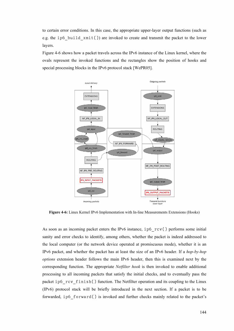
144

to certain error conditions. In this case, the appropriate upper-layer output functions (such as

e.g. the ip6_build_xmit()) are invoked to create and transmit the packet to the lower

layers.

Figure 4-6 shows how a packet travels across the IPv6 instance of the Linux kernel, where the

ovals represent the invoked functions and the rectangles show the position of hooks and

special processing blocks in the IPv6 protocol stack [WePR05].

Figure 4-6: Linux Kernel IPv6 Implementation with In-line Measurements Extensions (Hooks)

As soon as an incoming packet enters the IPv6 instance, ip6_rcv() performs some initial

sanity and error checks to identify, among others, whether the packet is indeed addressed to

the local computer (or the network device operated at promiscuous mode), whether it is an

IPv6 packet, and whether the packet has at least the size of an IPv6 header. If a hop-by-hop

options extension header follows the main IPv6 header, then this is examined next by the

corresponding function. The appropriate Netfilter hook is then invoked to enable additional

processing to all incoming packets that satisfy the initial checks, and to eventually pass the

packet ip6_rcv_finish() function. The Netfilter operation and its coupling to the Linux

(IPv6) protocol stack will be briefly introduced in the next section. If a packet is to be

forwarded, ip6_forward() is invoked and further checks mainly related to the packet’s

145

lifetime, its source and destination addresses, and the outgoing link’s MTU are performed.

Packets to be delivered locally are passed to ip6_input() (either directly or through

ip6_mc_input() in case of multicast) which in turn invokes ip6_input_finish()

over the relevant Netfilter hook. This latter function examines any extension headers that

might be present in an IPv6 packet other than hop-by-hop options which have already been

processed126, and it then passes execution to the appropriate handling routine, based on the

packet’s transport protocol.

Packets created locally and passed from the transport layer to the IPv6 instance can be sent via

different functions, each one specialised for a specific use127. An example of such functions is

ip6_xmit() which accepts a packet from the TCPv6 implementation, it allocates space (if

necessary) to the packet data area of the corresponding socket buffer, and then sets the

individual parameters in the IPv6 header. After passing the appropriate Netfilter call, a route

for the packet is calculated, and it is then passed to ip6_output() and eventually to

ip6_output_finish(), which ultimately passes the packet to the transmit functions of

the lower layers to be sent over the network link [WePR05, Herr00, Kern05].

4.4.2.1 The Netfilter Hooks in the Linux Kernel

Netfilter [Netf05] is a general framework built within the Linux 2.4 (and 2.6) kernel series

that enables packet filtering and manipulation as datagrams traverse the networking code of

the Operating System128. Packet filtering is primarily used for control and security over the

flow of network traffic, and is based on the examination of numerous fields in a datagram’s

protocol headers which results in deciding the fate of the entire packet. The Netfilter

126 This detail regarding the processing of the IPv6 extension headers is of particular importance, since

it demonstrates how a general-purpose (Linux) IPv6 implementation reflects the protocol specification.

The IPv6 specification states that all extension headers (other than hop-by-hop options which are

processed en-route) are only processed by the packet’s explicit destination nodes (sections 3.6.1, 3.6.2,

and 3.7). Accordingly, the protocol implementation parses hop-by-hop options that might be present in

all incoming packets as soon as they pass the initial IPv6 error checks. On the contrary, all other

extension headers that might be present in a datagram are only processed for packets that are to be

delivered locally, just before they are passed to the higher-layer handling routines or to the matching

raw IPv6 socket. 127 The listing and description of these functions is outside the scope of this thesis. 128 Packet filtering had been implemented in Linux since its early kernel versions. Netfilter and the

accompanying tools are its latest evolution.

146

framework can provide for among others network address and port translation, stateful and

stateless packet filtering, sophisticated firewalling and other packet mangling129.

The two building blocks of the framework are the so-called Netfilter hooks which reside in the

kernel’s networking code and provide a mechanism to manipulate IP packets at different

positions of the IP instance, and a user-space tool (iptables) to essentially register and control

the kernel filtering rules [Russ02a]. Netfilter hooks have been defined for both IPv4 and IPv6

(and DECnet) at specific points in a packet’s traversal of the protocol stacks. When Netfilter

modules are loaded into a running Linux kernel, the hooks enable the execution of the

additional processing functions. Calling a Netfilter macro from within the kernel’s networking

functions with the packet (socket buffer) and the hook number results in the registered packet-

filter functions to be executed and decide whether the packet should be accepted for further

processing in the kernel, dropped, be queued for user-space processing, or its contents should

be somehow manipulated/altered [Russ02b]. If there is no registered filter-function for the

specific protocol and hook number, execution will immediately jump to the following kernel

networking function which is passed as a parameter to the Netfilter macro. As it can be seen in

Figure 4-6, five distinct Netfilter hooks have been defined for IPv6 to filter packets at

different, well-defined positions of the IPv6 instance, conceptually covering all the different

‘states’ of a packet while it traverses the kernel’s networking code. The

NF_IP6_PRE_ROUTING hook resides in ip6_rcv() and it passes all incoming packets to

the Netfilter framework before they are processed by the routing code. The additional

processing enabled by this hook can be meaningfully used for network address translation and

detection of certain denial-of-service attacks. After a packet is handled by the routing code

that decides whether it is destined for another interface or a local process130, the

NF_IP6_LOCAL_IN hook passes to the framework packets destined to the local system, just

before they are delivered to an awaiting process (if any). Calling this hook is the only task of

ip6_input(). Alternatively, if the packet is destined for another interface, the framework

is called again for NF_IP6_FORWARD from within ip6_forward(). The

NF_IP6_LOCAL_OUT hook is called from within the different transmit functions that handle

higher-layer outgoing packets that are created locally. The final Netfilter hook is the

NF_IP6_POST_ROUTING which is called from within ip6_output() to filter all

outgoing packets just before they leave the local system over a network device.

129 Examples of packet mangling provided by the Netfilter framework include altering field values in

the various packet headers, such as, for example, the advertised Maximum Segment Size (MSS) in a

TCP SYN packet, and the Type-of-Service (ToS) field in the IP header. 130 The packet might be dropped at this stage, if it is unroutable.

147

Linux kernel modules can register to listen to any of these five hooks, and when these are

called from the core networking code, the registered modules are free to manipulate the

packet, according to a set of relative priorities [Russ02b]. The modules then instruct Netfilter

to take a specific action out of a well-defined set of actions. Only if all the registered functions

at a specific hook return an accept value, the traversal of the packet within the IPv6 instance

can continue with the immediately following core networking function.

4.4.2.2 The In-line Measurement Hooks in the Linux Kernel

At a system level, the in-line measurement functionality and operation have several common

characteristics with the Netfilter framework. In principle, the direct (in-line) measurement

through the addition of indicators within selected outgoing IPv6 packets and the observation,

recording, and possibly amendment of existing measurement data within incoming packets

can be seen as special functions within the general packet filtering and mangling concept

provided by Netfilter under Linux. Indeed, the Netfilter framework could have been used as

the basis for implementing the in-line measurement modules by registering additional special-

purpose functions to the IPv6 Netfilter hooks of interest, and assigning them a priority relative

to filtering, mangling, connection tracking, and the rest of the Netfilter operations.

Additionally, the Netfilter framework could have been used to queue incoming and outgoing

IPv6 packets at certain hooks and pass them onto user-space for asynchronous131 packet

handling. Using this facility, the in-line measurement modules could have adopted a more

straight-forward, system and language-independent implementation as user-space processes,

decoupled from the kernel operation. However, as it has been raised in section 4.4, such user-

space implementation is not ideal, neither for high-speed processing nor for demonstrating the

measurement modules’ operation on network nodes where a ‘user-space’ might simply not be

present.

For similar reasons of minimisation of the inter-operational assumptions regarding the system

operating environment of the in-line measurements modules, it was preferred for the prototype

to keep its reliance on existing frameworks as well as its dependencies on add-on components

at a bare minimum.

Finally, the in-line measurement instrumentation could have been hard-coded within the

kernel’s IPv6 instance, directly embedding the additional functionality at appropriate points in

the protocol stack to provide for the necessary processing of the measurement options within

the IPv6 Destination Options headers. However, such approach would have been more

appropriate for already standardised options that would start being widely supported in IPv6

131 The kernel does not wait while the packet is handled in user-space. At some later time, the packet

will be re-injected in the kernel and processing will continue [Russ00].

148

implementations, and potentially used by applications. Instead, the in-line measurement

prototype has been designed and implemented as an independent set of self-contained

modules of code, whose actual interference with the core kernel code only occurs at two

certain places, in the form of call-back hooks. As it can be seen from Figure 4-6, two hooks

have been put in place to pass control to the measurement modules as soon as packets enter an

instrumented node and just before they are passed to the lower layer transmit functions,

respectively. IP6_INPUT_PACKETS resides within ip6_rcv() and is called as soon as

an incoming packet is delivered to the IPv6 instance and has passed the initial versioning and

length error checks. IP6_OUTPUT_PACKETS resides in ip6_output_finish() and is

called just before an outgoing packet is passed to the lower layer for transmission over a

network device. These two hooks that operate on incoming and outgoing packets respectively

are arrays of certain length that consist of pointers to functions, each one taking as an

argument the socket buffer that represents and manages the packet in question. When no

measurement modules are loaded, the arrays contain null pointers and consequently the kernel

only has to perform one extra comparison over the elements of each array. When a

measurement module is loaded in the kernel, it replaces the first available pointer in the

respective input or output array132 with its call-back function which then becomes part of the

kernel’s IPv6 instance. Similarly, when the module is unloaded, the corresponding pointer is

set back to null. In this manner, incoming and outgoing IPv6 packets are passed to all loaded

modules that have registered their call-back function.

As will become evident in the following section, minimal measurement modules have been

implemented to either insert, or observe and record a particular measurement indicator.

Hence, the arrays of pointers (instead of a single function pointer) allow for more than one

module to operate simultaneously either on incoming or outgoing packets, by registering their

processing routines with an entry of the corresponding array. Of course this comes at the cost

of the kernel performing more comparisons over the entries of each array to identify how

many modules have currently registered their functions with the kernel, and therefore, the

number of entries in each array needs to be carefully chosen. For the purposes of this

prototype implementation each array has two entries, essentially only marginally burdening

the kernel with an additional (second) comparison133.

132 Depending on the operation of the loaded module, it will register itself either with the

IP6_INPUT_PACKETS or the IP6_OUTPUT_PACKETS hook (array), as described in section 4.4.3. 133 One extra comparison in the kernel code is the minimum additional operation required to install a

hook in this manner [Herr00]. Also, this is the minimum permanent overhead introduced to the kernel

while no modules are installed.

149

4.4.3 Measurement modules as Linux Dynamically Loadable Kernel

Modules (LKM)

It has been highlighted in section 4.4 that a kernel-level implementation of the core in-line

measurement components was preferred, due to their real-time operation on the data path and

the direct performance implications on the IPv6 traffic flow of the instrumented nodes.

Following this design choice, under Linux, the code could have been built directly into the OS

kernel or it could have been designed as (a set of) Loadable Kernel Modules (LKM)s that can

be linked to a running kernel at runtime. The former would have been a conceptually much

simpler approach, since it would only require the placement of the additional processing

routines within the appropriate core functions of the kernel’s IPv6 instance. In particular, the

additional measurement TLV-encoded options (described in sections 3.8.1 and 3.8.2) would

have to be defined in the inet6 implementation definitions, and then the corresponding

handling functions would have to be added in the IPv6 extension header processing blocks of

the kernel and linked to the kernel’s IPv6 destination options list. However, this approach

would have to make semi-permanent changes to the OS kernel and the overall implementation

and debug process would have been heavyweight and time-consuming, since the entire kernel

would have to be re-compiled, installed and rebooted for every alteration in the code. At the

same time, such direct coupling with the implementation of a steady release of the Linux

kernel would not have been the most appropriate for an experimental prototype whose

protocol-dependent parameters and operation have not passed any official standardisation

process. Most importantly though, this unified and, in a way, monolithic implementation of

the measurement functionality would conflict with the idea of providing a highly modular

instrumentation system, to minimise the additional processing requirements by loading the

appropriate components as and when required to undertake specific measurement actions.

Designing the measurement components as a set of LKMs offers a number of advantages over

the integrated approach which will be briefly outlined in the remainder of this section.

Generally, LKMs extend the functionality of the kernel without the need to re-compile,

reinstall, or even reboot the system, offering a much safer and easier mechanism for a (super)

user to build, install and remove functionality which operates as part of the kernel code. The

modules are components of the operating system which Linux allows to dynamically load and

unload, and be linked into a running kernel at any time after the system has booted. Once a

Linux module is loaded is as much a part of the kernel as any normal kernel code. This

functionality of dynamically loading code as and when it is needed, makes the kernel very

flexible and keeps its size to a minimum, since there is a portion of the kernel that remains in

memory constantly and implements the most frequently-used processes, but others are

implemented as modules and are only loaded on demand. Although there is a slight

150

performance and memory penalty associated with LKMs (in comparison to the core kernel

code) mainly due to the extra data structures and a level of indirection introduced, they

provide the ‘golden section’ between large and complex monolithic kernels and small but less

efficient micro-kernel structures [Rusl99, WePR05].

LKMs can access and use resources exported by the kernel in its symbol table, which is

updated and enhanced with resources or symbols exported by loaded modules. Hence, newly

loaded modules use the same mechanism to access resources exported either by the kernel

itself or by other, previously loaded modules.

In contrast to normal programs that run as user-space processes, LKMs always begin with an

initialisation function that sets up the kernel to run the module’s functions when needed. This

entry function typically either registers a handler for something with the kernel, or it replaces

one of the kernel functions with its own code134. It then returns, and the module waits until its

code is invoked by the kernel. The modules end by calling a cleanup function which should

un-register any functionality registered by the initialisation function.

Further detailed operational description of the Linux LKM concept and its benefits is outside

the scope of this thesis. The interested reader can find additional information in [Rusl99,

Herr00, SaPo03].

For the in-line measurement prototype, the Linux LKM mechanism is particularly suitable

since it provides the basis for the measurement components to be implemented as separate

modules and operate as part of the OS kernel, hence minimising the performance overhead

issues due to context switching between kernel and user space. At the same time, enabling

selected modules to be loaded and hence linked to the kernel (and unloaded, respectively) as

and when required with minimal disruption to the operating environment, it serves well the

purposes of an add-on mechanism which will minimise the actively used processing logic and

its operational overhead, by only using the necessary components to perform a certain type of

measurement. This approach leads to a lightweight instrumentation mechanism whose

different components have a well-defined appositeness and role, and can be explicitly

instantiated135 both at a node-local level as well as under a wider distributed measurement

system as it has been discussed in sections 4.2 and 4.3.

However, the Linux kernel does not always export the variables a LKM may need to access.

In this particular case, the measurement modules need to be able to access and process either

134 As representative examples, the in-line measurement modules operate by registering a handler with

the kernel, whereas the Netfilter framework is designed to invoke their additional packet-handling

routines and upon completion to call the original kernel function. 135 Individual components can be, for example, explicitly ‘turned on and off’ on demand, upgraded,

installed at and/or removed from an instrumented system.

151

the incoming or the outgoing packets, as these travel through the IPv6 instance’s receive and

transmit functions, respectively. The LKM-based implementation of the measurement

modules requires a few minor modifications to the kernel to allow access to the packet

structure (sk_buff) within the appropriate functions of the networking code. The kernel will

have to be recompiled and installed only once, and the modules will then take advantage of

these modifications when they are loaded to take control over the core networking code,

perform their additional operations, and return the packet to complete its IPv6 stack traversal.

These modifications have been implemented in the form of the two hooks described in the

previous section (4.4.2.2).

At a protocol level there are a number of different places where the in-line measurement

modules could have been hooked in. Since their functionality is IPv6-specific, it is

conceptually the right place for the hooks to reside within the protocol’s routines136, so that

the strict layering of the TCP/IP model is retained. Additionally, as it has been discussed in

section 3.7 and, at an implementation level highlighted in section 4.2, the in-line measurement

modules can perform two major operations, depending on the role of an instrumented system

during a particular measurement activity and topology. For the purposes of a unidirectional

multi-point measurement, an instrumented system can either add measurement information to

outgoing traffic by constructing and inserting the appropriate IPv6 destination options

headers, or observe (and possibly amend) already created measurement headers carried within

the incoming datagrams. The two in-line measurement hooks that have been added in the

Linux kernel’s IPv6 input and output routines provide exactly this necessary access to the

respective measurement modules. Based on the IPv6 specification, extension header creation

should only take place at a packet’s originator node, and extension header processing should

only take place at the packet’s explicitly identified intermediate or/and ultimate destination

[DeHi98]. Hence, according to the standard, the hooks for the measurement modules would

reside within the local packet delivery and local packet creation blocks of the IPv6 instance,

respectively. Those are, approximately, where the EXTENSIONS building blocks are shown in

Figure 4-6 to either process or create the IPv6 extension headers. However, it was decided that

the hooks should pass control to in-line measurement modules as soon as incoming packets

are delivered to the IPv6 instance, and just before outgoing packets are passed to lower level

transmit functions. The main reasons that influenced this decision include the desire for

inherently powerful instrumented nodes that are able to do certain measurement extension

header processing to potentially any kind of traffic handled by their IPv6 instance.

136 Having the modules operating at the network device driver, the generic network device functions, or

the transport level would break the layering of the protocols and/or could potentially be applicable for

affecting only specific traffic types.

152

IP6_INPUT_PACKETS pass incoming traffic to the measurement modules prior to any other

packet filtering, mangling, and routing operations, allowing an instrumented system to

perform a direct measurement observation not only to traffic delivered locally but also to

traffic routed through that node. Similarly, IP6_OUTPUT_PACKETS resides at a single

place, where all outgoing IPv6 traffic passes through, facilitating measurement extension

header creation for traffic originated locally as well as for routed traffic that originated at

different end-systems. This invocation of the measurement modules from within ip6_rcv()

and ip6_output_finish() respectively, might at first sight be seem as violating the

strict IPv6 processing rules, however, it actually demonstrates the end-to-end as well as the

intermediate path applicability of the technique (as discussed in section 3.9) through a simple

and generic implementation. True end-systems can instrument their locally-originated traffic

with measurement extension headers at the source, and process these headers for locally-

delivered traffic at the destination of an end-to-end instrumented path. At the same time, this

implementation demonstrates how the same mechanism can provide for multi-point

measurement over a network domain, where packets are instrumented at an ingress node and a

direct measurement observation occurs at an egress point, before traffic is further forwarded to

its ultimate destination. At an implementation level, the seamless inter-operation with non-

supportive nodes is demonstrated by the internal encoding of the options that ensures an

option is skipped if not supported (section 3.8), as well as by the Linux example of a generic

IPv6 implementation, which ensures that common nodes process destination options extension

headers only for locally delivered packets. Well-identified and properly instrumented systems

can implement in-line measurement as an additional functionality by only making node-local

changes to the per-packet processing, and without influencing how the packet is treated by the

rest (not instrumented) network nodes along its end-to-end path.

The following sections describe the detailed operation of the in-line measurement modules,

which differs depending on whether the module operates at the source or the destination of an

instrumented path, and also on the type of measurement metric a module implements.

Specifically, the focus stays on the prototype implementation of the two TLV-encoded

measurement destination options described in sections 3.8.1 and 3.8.2. An instrumented path

is defined here as the set of links between which an in-line measurement operation takes

place. The source of an instrumented path is the network node where the IPv6 destination

options header containing the corresponding in-line measurement options is created and

piggybacked to a selected datagram. The destination of an instrumented path is the network

node where a packet carrying a measurement extension header is examined, the measurement

data is observed and/or amended, and the measurement header can be enhanced, and/or

removed. The source and destination nodes of an instrumented path may or may not be the

true end points of the datagram’s end-to-end Internet path.

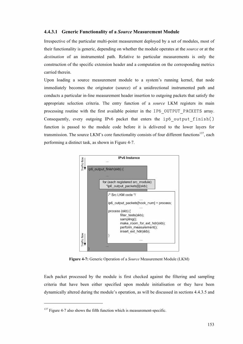
153

4.4.3.1 Generic Functionality of a Source Measurement Module

Irrespective of the particular multi-point measurement deployed by a set of modules, most of

their functionality is generic, depending on whether the module operates at the source or at the

destination of an instrumented path. Relative to particular measurements is only the

construction of the specific extension header and a computation on the corresponding metrics

carried therein.

Upon loading a source measurement module to a system’s running kernel, that node

immediately becomes the originator (source) of a unidirectional instrumented path and

conducts a particular in-line measurement header insertion to outgoing packets that satisfy the

appropriate selection criteria. The entry function of a source LKM registers its main

processing routine with the first available pointer in the IP6_OUTPUT_PACKETS array.

Consequently, every outgoing IPv6 packet that enters the ip6_output_finish()

function is passed to the module code before it is delivered to the lower layers for

transmission. The source LKM’s core functionality consists of four different functions137, each

performing a distinct task, as shown in Figure 4-7.

Figure 4-7: Generic Operation of a Source Measurement Module (LKM)

Each packet processed by the module is first checked against the filtering and sampling

criteria that have been either specified upon module initialisation or they have been

dynamically altered during the module’s operation, as will be discussed in sections 4.4.3.5 and

137 Figure 4-7 also shows the fifth function which is measurement-specific.

154

4.4.3.6. If these are satisfied, the next function examines whether the socket buffer assigned to

manage the particular outgoing packet has enough space in its headroom area to accommodate

for the size of the IPv6 extension header or option related to that measurement. If necessary,

the headroom is grown138 by the appropriate number of bytes and the data area is expanded

(pushed) towards the head of the socket buffer accordingly (Figure 4-5).

At this stage, there are some implementation-dependent and IPv6 related aspects that need to

be taken into consideration, which would probably need to be re-visited under different

realisations of an in-line measurement system, and as IPv6 will operationally evolve and

different extension headers and options will be standardised. For this particular prototype

implementation, the in-line measurement destination options processing is treated in a semi-

autonomous manner since it is not fully integrated to the implementation of the IPv6 instance

(as discussed in the previous section). More specifically, outgoing packets are passed to the

source module after their core IPv6-level processing has been carried out by the kernel, and

hence, there is a possibility that other extension headers have already been created by an

application or by the kernel itself and encoded in the packet. Therefore, it is not sufficient for

the source LKM to simply create and add its measurement-specific destination options header

immediately after the main IPv6 header. Rather, it needs to examine the contents of the packet

structure in order to identify where in the packet and how to encode its own extension headers.

In the simplest and most popular case (due to lack of standardised and widely used IPv6

options) where no extension headers have been encoded in the packet, then a destination

options header that will encapsulate the measurement-specific option is created and encoded

between the IPv6 and the upper-layer header.

If other extension headers already exist in the packet, then a destination options header is

encoded according to the IPv6 specification recommended order [DeHi98]. Since it is

desirable for the prototype to accommodate for both intermediate and end-to-end path

measurements, the options produced by the source module should potentially be able to be

examined by intermediate as well as the ultimate destination of the packet. Hence, the

destination options header carrying the measurement options should only be preceded by a

present hop-by-hop options header, and itself should precede any other extension headers

(section 3.6.1). A slightly more complicated yet rarer case occurs if the packet already

contains a destination options extension header carrying other application or kernel-specific

options. Then, the measurement-specific option produced by the source module needs to be

encoded within the same destination options header. The module code must add the option at

the end of the existing header, and also ensure that it is aligned at its natural boundaries. This

138 Actually, a new socket buffer with sufficient headroom space is created to handle the packet. The

data part of the old socket buffer is then copied to the new one.

155

latter scenario might prove to be of rare occurrence, since it is assumed that when option-

bearing headers are present they usually carry only one option [DeHi98, StTh98].

After this decision-making process, the main IPv6 header and any other extension headers that

might precede the measurement-specific options are moved forward in the packet structure in

order to allow space for the extension header to be inserted, and the socket buffer’s network

header pointer (Figure 4-4) is updated accordingly.

The source LKM has then to perform a node-local computation of the measurement indicator

of interest, and to construct the relevant option and the destination options extension header

that will encapsulate the measurement data. The extension header is then injected to the

packet and the necessary fields of the packet’s headers are updated accordingly. The payload

length field of the main IPv6 header is updated to include the recently added data and the next

header field of the preceding header is updated to reflect the current state of headers within

the packet. Upon completion of these operations, the module then returns control back to the

kernel’s IPv6 instance which in turn passes the enhanced socket buffer for transmission to the

lower layers. If at any time during the module’s execution some operating condition139 is not

satisfied, then the packet is returned to the kernel unmodified.

4.4.3.2 General Functionality of a Destination Measurement Module

An in-line measurement destination module implicitly marks an end-point of an instrumented

path, where the indicators carried within specific destination options headers of incoming

datagrams are examined and possibly amended to evolve to a multi-point measurement

observation. When the destination LKM is linked with the node’s kernel, then the node is

capable of performing a multi-point measurement solely based on information carried within

an instrumented IPv6 datagram and on node-local computations.

Similarly to the source module’s operation, the destination LKM registers its main processing

routine with the first available pointer in the IP6_INPUT_PACKETS array. As soon as an

incoming packet enters the main IPv6 routine from the lower layers and satisfies the initial

sanity and error checks, it is then passed to the module code from within ip6_rcv(), before

it is further processed and internally routed by the protocol instance.

There are two main conceptual differences between a source and a destination measurement

module. The most obvious is that the source module creates the extension header that will

encode a particular measurement option and injects it to the packet, and hence determines the

type of measurement to be performed. In contrast, the destination module examines all

incoming packets to find a particular extension header of interest. If this exists, the module

can perform a simple observation on the existing measurement data, or a complementary

139 Such conditions can include the non-matching of a filtering parameter or a failed skb operation.

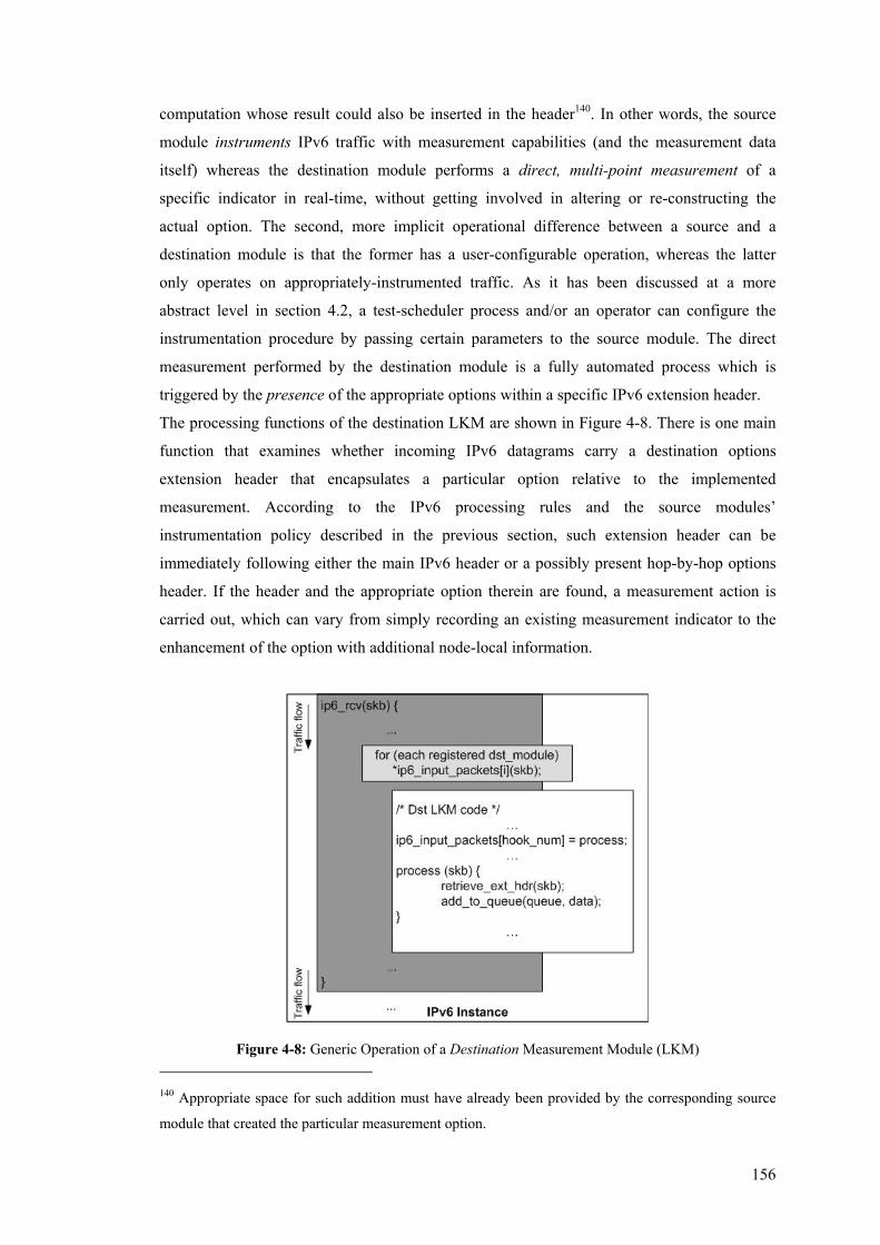
156

computation whose result could also be inserted in the header140. In other words, the source

module instruments IPv6 traffic with measurement capabilities (and the measurement data

itself) whereas the destination module performs a direct, multi-point measurement of a

specific indicator in real-time, without getting involved in altering or re-constructing the

actual option. The second, more implicit operational difference between a source and a

destination module is that the former has a user-configurable operation, whereas the latter

only operates on appropriately-instrumented traffic. As it has been discussed at a more

abstract level in section 4.2, a test-scheduler process and/or an operator can configure the

instrumentation procedure by passing certain parameters to the source module. The direct

measurement performed by the destination module is a fully automated process which is

triggered by the presence of the appropriate options within a specific IPv6 extension header.

The processing functions of the destination LKM are shown in Figure 4-8. There is one main

function that examines whether incoming IPv6 datagrams carry a destination options

extension header that encapsulates a particular option relative to the implemented

measurement. According to the IPv6 processing rules and the source modules’

instrumentation policy described in the previous section, such extension header can be

immediately following either the main IPv6 header or a possibly present hop-by-hop options

header. If the header and the appropriate option therein are found, a measurement action is

carried out, which can vary from simply recording an existing measurement indicator to the

enhancement of the option with additional node-local information.

Figure 4-8: Generic Operation of a Destination Measurement Module (LKM) 140 Appropriate space for such addition must have already been provided by the corresponding source

module that created the particular measurement option.

157

The destination module then extracts the packet information required by the higher-level

applications that will post-process and analyse the measurement data to implement the various

performance metrics. This obviously includes the contents of the measurement-related IPv6

option, but depending on the implementation, it can also include additional network and

transport layer packet header information. The extracted data is stored into a FIFO queue

structure whose elements can then be retrieved from user-space processes, as it will be

discussed in section 4.4.3.5.

The final operation of the destination LKM is to possibly remove the measurement option-

bearing header from the packet, in order to maintain complete transparency to the rest of the

system. The whole destination options header can be removed if and only if it solely contains

a single measurement option. In this case the next header field of the immediately preceding

header, as well as the payload length field of the main IPv6 header need to be adjusted

accordingly. In addition, the equivalent number of bytes can be truncated from the beginning

of the socket buffer associated with the packet.

However, the achieved transparency might not worth the processing overhead associated with

the additional operations. The module can pass the packet unmodified back to the kernel’s

IPv6 instance, which will ignore the measurement option if not supported according to the

encoding of its option type field (section 3.6.2).

4.4.3.3 The One-Way Delay (OWD) Measurement Modules

The in-line measurement prototype focuses on the implementation of time-related and packet

loss measurements using the corresponding IPv6 destination options defined in sections 3.8.1

and 3.8.2. The measurement functionality has been implemented as sets of source and

destination LKMs that create an appropriate option (and header) to carry the measurement

values of interest, and process packets containing a certain type of option, respectively.

The measurement modules that implement the creation and processing of the one-way delay

and one-way loss destination options have been built based on the common operational

concept of the source and destination LKMs described in the previous sections. However, the

nature as well as the actual realisation of each of these two types of measurement exhibits

some different characteristics, which are reflected by a number of distinct actions carried out

by the corresponding source and destination LKMs. This diversity demonstrates the number

of roles a module can have depending on the type of measurement being implemented.

The one-way delay source and destination LKMs implement a stateless per-packet

computation of the unidirectional delay between two instrumented systems in the network.

158

This two-point implementation which reflects the design of the relevant IPv6 destination

option141 can be considered as a special case of the multi-point in-line measurement technique.

The source LKM which establishes the beginning of an instrumented path follows the process

of creating the OWD TLV-encoded option and inserting it at the appropriate place between

the different headers of the datagram, as described in section 4.4.3.1. The TLV-specific static

values (option type, data length, etc.) are then inserted in the various fields of the option, and

the last action of the module is to obtain the node-local system time and encode it within the

corresponding timestamp fields. The kernel function do_gettimeofday() is used to read

out the clock counter structure (struct timeval) and return its two registers, one for the

number of seconds (tv_sec) from the start of the Unix era and one for the number of

microseconds (tv_usec). The two 32-bit integers are stored in the two source timestamp

fields of the OWD option, respectively. The other two 32-bit destination timestamp fields are

initialised to zero and the packet is then returned to the IPv6 instance and sent over the

network. The presence of a loaded destination module at either an intermediate hop or the

ultimate destination of the packet’s Internet path marks the end of the (two-point) one-way-

delay-instrumented path. As soon as an incoming packet is passed to the module code, if it

contains the OWD destination option, the node-local system time is obtained using the

previously described mechanism and the two 32-bit destination timestamp fields of the header

are filled with the seconds and microseconds values returned by the node’s clock counter

structure, respectively. For the purposes of this particular prototype implementation the

contents of the main IPv6 header, the OWD destination option and the transport layer header

are copied into a FIFO queue structure for further analysis. The overall OWD option-bearing

header is subsequently removed from the packet once the two-point timestamp computation

has been completed142.

It is worth mentioning here that, due to the positioning of the in-line measurement hooks in

the Linux kernel that pass execution to the measurement LKMs (section 4.4.2.2), this

software-based one-way delay measurement is a much better approximation of the packet’s

transmission time143 between two points in the network than timestamp measurements taken at

141 The OWD Option (section 3.8.1) encapsulates two timestamps with microsecond accuracy from the

source and the destination nodes (i.e. modules) of an instrumented path. Variations of this option could

potentially encode further timestamps to enable the calculation of the one-way delay between multiple

intermediate (destination) nodes of an instrumented path. 142 The IPv6 Destination Options header is removed if the already processed OWD option is the only

option encapsulated in the header. 143 The term “transmission time” between a source and a destination includes the serialisation,

propagation and queuing delays encountered by a packet at the intermediate links and hops.

159

the transport or the application layers, which are typically employed by most active

measurement infrastructures. Not only timestamping occurs within the kernel’s network layer

code, but just before the packet is copied to the data link medium (departure timestamp) and

as soon as it is received by the IPv6 instance (arrival timestamp), respectively. Hence, the

delay component of the processing time at the two instrumented systems that is implicitly

included in the OWD measurement is minimised, and a good software-based and medium

independent estimation of the actual one-way delay can be achieved. More accurate

timestamping could be implemented at the medium-specific device driver level, or and the

generic device functions level, however any of these approaches would violate the protocol

layering principles.

The one-way delay measurement requires relatively accurate but most importantly

synchronised clocks between the systems computing the departure and arrival timestamps of

the packets. Two of the most fundamental clock attributes that are not particularly reliable for

software clocks on commodity PC configurations are the rate and the offset, which indicate

the departure from true time at a given time. The former is of central importance for single-

point measurement observations (e.g. round-trip delay and packet inter-arrival times) whereas

offset synchronisation has generated more concern for measurements conducted by multiple

different nodes (e.g. one-way delay). Existing techniques used in inexpensive PCs to improve

clock synchronisation and hence accurate timestamping include the Network Time Protocol

(NTP), Global Positioning System (GPS)-based timing, and radio-based alternatives, which

all have their strengths and weakness. Usually, more accurate clock synchronisation requires

additional hardware and installation costs. Considerable research effort has been put into

providing adequate timestamping accuracy for the purposes of network measurements.

However, further discussion on clock synchronisation techniques and their relative advantages

and disadvantages is outside the scope of this thesis, and the interested reader is referred to

[Mill91, MiGD01, MoST99, Paxs98a, PaVe02].

4.4.3.4 The One-Way Loss (OWL) Measurement Modules

The One-Way Loss (OWL) measurement exhibits different characteristics from the one-way

delay measurement both at a conceptual and at an implementation level. The focus of the

prototype is on the two-point implementation of the one-way packet loss metric between two

end-points of an instrumented path that deploy the corresponding OWL source and

destination LKMs, respectively. However, in contrast to the stateless operation of the OWD

measurement modules, the two-point packet loss implementation needs to maintain common

state throughout the measurement period at both instrumented points, as this has been

explicitly discussed in section 3.8.2. This is mainly because packet loss is a metric related to a

particular series of packets rather than a self-contained per-packet characteristic, and it is

160

computed based on the presence and the sequence of a portion of network traffic, which is

used to infer the absence (the actual loss phenomenon), the retransmission, and the out-of-

order delivery of specific datagrams. Active measurement infrastructures that use software

processes to perform two-point packet loss measurements based on injected traffic can know

in advance the characteristics, the sequence and the number of the packets sent and received,

and can hence implement the metric on their portion of the traffic. However, this is not

possible for a measurement module that implements IP-based sequencing on existing network

traffic and it hence needs to employ its own criteria which will enable a meaningful

sequencing of somehow related IP datagrams.

The source OWL LKM maintains state using the notion of a flow (section 2.3.2) to create

groups of packets that share common characteristics among some of their protocol fields, at

their adjacent network and transport layer headers. Then, sequencing of packets processed by

the module is not absolute but relative to the flow each packet is identified to belong to. Upon

loading of the source LKM, a linked structure is initialised to hold a flow table for the entire

duration of the measurement. Each element of this structure represents a flow entry which can

be identified by the source and destination IPv6 address, the transport protocol, and the

transport protocol’s source and destination port numbers of each observed packet. The flow

element also contains two 32-bit integers, one to store the sequence number of the last packet

seen to belong to the specific flow, and one to store the time this last packet was processed by

the instrumented node. The granularity of the flow table can be made coarser, either at

initialisation of the module or at runtime, by replacing any of 5-tuple’s elements with a

wildcard filter144.

The OWL-specific operations performed by the source module upon receiving an IPv6

outgoing packet through the in-line measurement hooks include the insertion of the static

values of the TLV, the identification of the packet’s flow, and ultimately, the computation and

insertion of the IP-based packet’s sequence number to the TLV’s appropriate field. The packet

headers’ fields that correspond to the flow identification tuple are compared against the entries

of the module’s flow table. If an identical flow entry exists, and the time between the

processing of the previous packet belonging to the same flow and this last packet does not

exceed a certain threshold, then the sequence number stored for this flow entry is incremented

by one and inserted to the packet’s OWL TLV; the timestamp of the specific flow entry is

updated accordingly. Otherwise, if such a flow entry does not exist or if its timeout value has

expired, then either a new flow entry is created or the sequence number of the existing entry is

reset to one (1).

144 The module can be configured, for example, to mark packets coming from or addressed to specific

IPv6 hosts/networks as belonging to the same flow.

161

The OWL destination LKM running on a node receives incoming IPv6 datagrams and if these

contain an OWL destination option, the module simply observes and stores the contents of the

main IPv6 header, the OWL destination option and the transport layer header into its

associated queue structure for post analysis, which will in turn compute any packet loss and/or

packet re-ordering and retransmission phenomena. The option-bearing header is then removed

from the packet structure if it solely contains the already processed OWL option.

The decision for the OWL destination module not to perform a real-time computation of the

packet loss metric was taken primarily for two reasons. The first is to emphasise that an in-

line measurement (destination) module can simply observe an appropriately-instrumented

packet, and record its contents for further offline processing. And second, to avoid the

additional overhead of re-determining the packet’s flow in real-time. This approach essentially

moves the concern of communicating common state information with the source OWL

module. Identical flow classification can be conducted by a higher-level measurement analysis

application. At the same time, by keeping the modules’ operation minimal, a potential broader

measurement framework could account for one-to-many relationships between source and

destination OWL modules. These can be operational scenarios under which multiple source

LKMs instrument packets that are examined by a single destination LKM and vice versa.

Measurement data populated by the destination modules can then be cumulatively processed

to identify losses over an overall network topology. In this case, the OWL TLV might also

need to be re-designed to include tags of the different nodes that instrumented and/or

processed different packets. However, such operational enhancement of the measurement

modules and their integration with network-wide measurement infrastructures are beyond the

purposes of this two-point prototype implementation, and further details are outside the scope

of this thesis.

4.4.3.5 Communicating Data between Measurement LKMs and User Processes

Irrespective of the particular type of measurement performed by a set of source and

destination modules, the LKMs need to deploy additional mechanisms to communicate the

necessary information from and to other components of the infrastructure at runtime.

For the purposes of this prototype implementation, two types of information are exchanged

between the measurement modules and higher-level (user-space) processes. Source modules

obtain configuration parameters mainly during initialisation but also at runtime, and

destination modules make the necessary per-packet data available for further measurement

and analysis processes.

As it has been already discussed, loading of a source LKM initiates the in-line measurement

activity and designates the instrumented node as the starting point of the measurement-

enabled path. The LKM is able to potentially process every single outgoing IPv6 packet, but

162

the decision of which traffic is actually instrumented with the in-line measurement destination

options is based on node-local policies passed as parameters to the module. A user-space

process that can run either locally or remotely such as the test scheduler described in section

4.2, links the source LKM to the running Linux kernel and configures the measurement

granularity by filling the entries of a control structure which is then passed to the module and

specifies the filtering and sampling parameters of the measurement process (discussed in

section 4.4.3.6). These configuration parameters can also be altered during the module’s

operation without the need to remove and then reload the LKM.

On the other hand, a destination LKM, when loaded, implicitly specifies the end of the

instrumented path that originates at the node running the corresponding source module. The

LKM which examines every incoming IPv6 datagram is loaded without any parameters being

explicitly specified since its measurement activity is triggered by the presence of the

appropriate options within a datagram (hence, only appropriately-instrumented packets are

actually being processed). However, when a packet is indeed eligible to be processed by the

destination LKM and its measurement-related header data is eventually extracted and stored to

the module’s FIFO structure, there needs to be a mechanism for this data to be exported to

user-space processes that will “consume” the measurement indicators to implement different

performance metrics and produce more aggregate results.

In short, source LKMs need to receive input from user-space whereas destination LKMs need

to pass their output to user-space processes, in real time. These I/O operations have been

realised by coupling a virtual character device with each measurement module and

implementing the corresponding read and/or write driver routines. Every LKM, upon

initialisation, registers itself with a character device file which has been created in advance145.

In order for multiple modules to simultaneously operate on the same system, an equal number

of distinct character device files are created to accommodate input and output data for each

module. Each module then implements the main functions to open, release, read from and

write to the virtual device, as necessary, when they are called from a user-space process. The

standard roles of read and write are reversed in the kernel, and therefore read functions are

used for output from the module (and the character device) whereas write functions are used

for input to the module [SaPo03].

Each source LKM implements a function which, when called from a user process, it

overwrites (through the character device file) the entries of the module’s control structure,

and consequently, it alters the granularity of the measurement process. A user-space

application can hence specify different filtering and sampling parameters on demand to take

145 This is the most convenient way in order for the modules as well as the applications to know which

character device needs to be accessed.

163

immediate effect while the module is loaded, and then copy them from the user data segment

to the kernel data segment, using the appropriate Input Output ConTroL (IOCTL) call146.

Accordingly, each destination LKM running at the other end of an instrumented path,

implements a function called when a user process attempts to read from the character device

file registered by the module. This function copies to the caller’s (process) buffer the bytes

that correspond to the first (oldest) element of the FIFO queue holding the measurement-

related header data of each processed incoming IPv6 packet. It subsequently frees the space

occupied by this element in the memory-resident queue. This queue maintained by each

destination module has a fixed maximum number of bytes that it can accommodate and when

its capacity is reached, measurement data from subsequent packets is dropped. It hence

becomes evident that especially for certain types of measurement (such as e.g. packet loss), a

user-space process need to issue read calls to the corresponding character device file at a rate

which can accommodate the rate of instrumented packets arriving at the destination LKM.

The measurement granularity dictated by the corresponding source LKM can also influence

the rate of arrival of instrumented packets at the destination node/module.

However, discussion on such rate synchronisation issues between the measurement modules

and the higher-level applications is outside the scope of this thesis147.

4.4.3.6 Measurement Scope, Granularity and Cost Reduction: Partial Byte

Capture, Filtering and Sampling

The combinations of source and destination LKMs deployed to implement a certain

performance computation, are able to instrument IPv6 datagrams at configurable levels of

granularity. The modules exploit three main strategies to reduce the processing load imposed

on the instrumented nodes, as well as the volume of measurement data, both of which,

together with the inherent properties of the in-line technique can reduce significantly the costs

of the measurement process. Partial byte capture, packet filtering, and packet sampling are 146 IOCTL is a special function that handles read, write and communication with a device through a

single file descriptor, and can be used to pass almost anything from a process to the kernel, such as in

this case, a pointer to a structure. 147 As an example, an extreme upper bound requirement can be for an application not to loose packets

when the destination module operates at full line speed with minimum-sized packets. One can consider

a software implementation on a commodity PC able to process minimum-sized IP packets at 100 Mb/s

Ethernet link. Studies have shown that the smallest popular MTU is around 44 bytes for TCP control

and acknowledgement segments (which, using IPv6 would be 64 bytes). If the node is able to actually

process 64-byte (512-bit) packets at 100 Mb/s, and assuming that the destination measurement module

would process every single packet (highly unlikely), then the application would have to read the queue

every 5.12 µsec, in order to make sure no packets will be dropped.

164

mainly used by measurement systems that operate under un-controlled conditions and observe

network traffic passing through a link (as discussed in section 3.5.2).

Partial byte capture has been implemented by each destination LKM which concludes a two-

point in-line measurement, and passes the related per-packet data to applications for further

processing and analysis. After performing a node-local computation or a simple observation

on an incoming already instrumented IPv6 datagram, the module then only stores partial

header data to be passed to user-space processes. This data could in theory be as little as 8 or

even 4 bytes per packet (for one-way delay and loss, respectively) in case the module

performed the complete computation in real-time and only stored its final outcome. For the

purposes of this prototype, however, the destination module only performs the time-critical

measurement actions and stores all the network and transport layer headers of the packet in its

memory-resident queue. This can result in capturing from 56 to 84 bytes per instrumented

packet148, which are already a fraction of the overall traffic passing through the node and can

be further reduced when measurement data is written on disk (section 4.4.4). In addition, it is

important to note that the multi-point nature of the in-line technique enables this amount of

per-packet data to be captured (stored) at a single point in the network, while containing all

the necessary information for a two-point measurement. This property essentially reduces

almost in half the amount of measurement-related data that would be necessary in order to

perform a two-point measurement using conventional passive monitoring techniques149, and it

obviates the need for shipping and correlation of per-packet data from multiple points in the

network, probably over the network itself.

Although the in-line measurement modules observe the operational IPv6 traffic passing

through certain network nodes in a similar manner to passive monitoring approaches, the

actual instrumentation can be targeted on certain subsets of the IPv6 traffic. Choice of a

particular subset of traffic to be instrumented with the in-line measurement headers depends

on the filtering and sampling parameters configured upon loading or during operation of a

source measurement module, which is the initiator of the in-line measurement activity over a

specific instrumented path. The relevant destination LKM will then only process packets

encapsulating the appropriate IPv6 destination options; hence, it will operate on the same

148 For this prototype implementation, the best case scenario is an instrumented UDP/IPv6 (8 + 40

bytes) packet carrying an OWL destination option (8 bytes) in a single option-bearing extension header;

the worst case scenario is a TCP/IPv6 (20 + 40 bytes) packet carrying an OWD destination option (24

bytes). 149 The in-line measurement technique is only compared and contrasted to passive monitoring

techniques here, because they also operate on the actual network traffic. Active measurement

techniques operate on special-purpose traffic under controlled conditions.

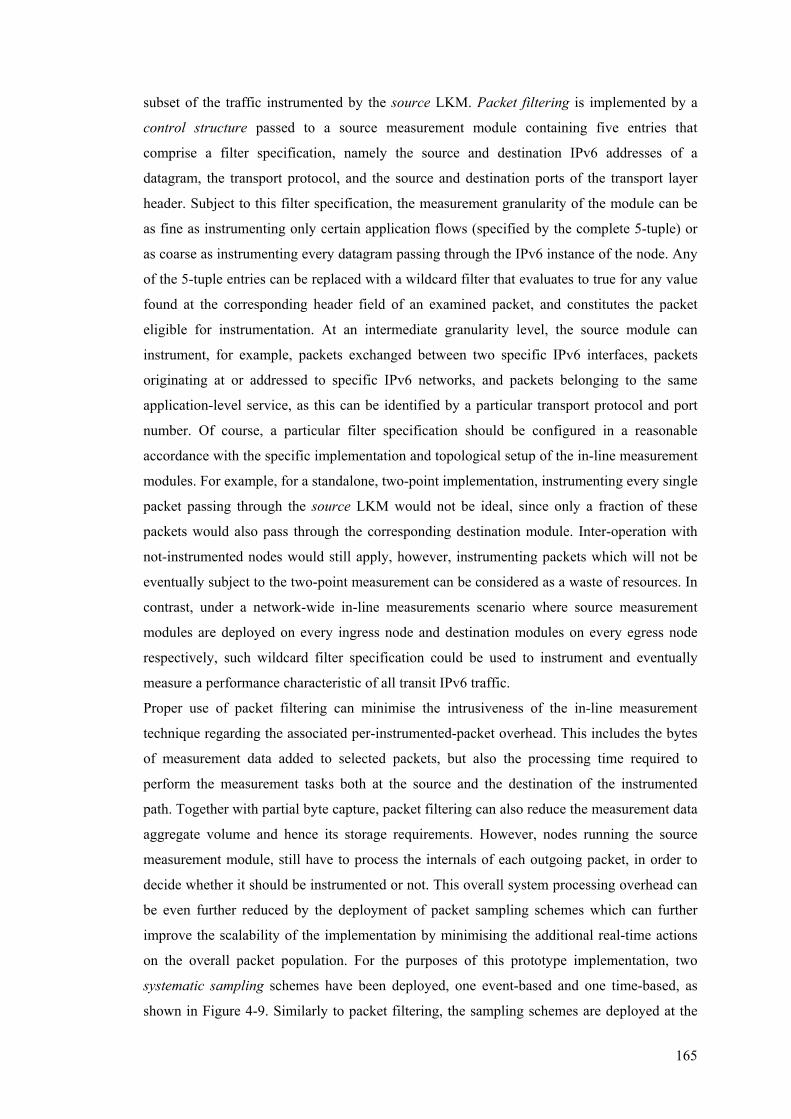
165

subset of the traffic instrumented by the source LKM. Packet filtering is implemented by a

control structure passed to a source measurement module containing five entries that

comprise a filter specification, namely the source and destination IPv6 addresses of a

datagram, the transport protocol, and the source and destination ports of the transport layer

header. Subject to this filter specification, the measurement granularity of the module can be

as fine as instrumenting only certain application flows (specified by the complete 5-tuple) or

as coarse as instrumenting every datagram passing through the IPv6 instance of the node. Any

of the 5-tuple entries can be replaced with a wildcard filter that evaluates to true for any value

found at the corresponding header field of an examined packet, and constitutes the packet

eligible for instrumentation. At an intermediate granularity level, the source module can

instrument, for example, packets exchanged between two specific IPv6 interfaces, packets

originating at or addressed to specific IPv6 networks, and packets belonging to the same

application-level service, as this can be identified by a particular transport protocol and port

number. Of course, a particular filter specification should be configured in a reasonable

accordance with the specific implementation and topological setup of the in-line measurement

modules. For example, for a standalone, two-point implementation, instrumenting every single

packet passing through the source LKM would not be ideal, since only a fraction of these

packets would also pass through the corresponding destination module. Inter-operation with

not-instrumented nodes would still apply, however, instrumenting packets which will not be

eventually subject to the two-point measurement can be considered as a waste of resources. In

contrast, under a network-wide in-line measurements scenario where source measurement

modules are deployed on every ingress node and destination modules on every egress node

respectively, such wildcard filter specification could be used to instrument and eventually

measure a performance characteristic of all transit IPv6 traffic.

Proper use of packet filtering can minimise the intrusiveness of the in-line measurement

technique regarding the associated per-instrumented-packet overhead. This includes the bytes

of measurement data added to selected packets, but also the processing time required to

perform the measurement tasks both at the source and the destination of the instrumented

path. Together with partial byte capture, packet filtering can also reduce the measurement data

aggregate volume and hence its storage requirements. However, nodes running the source

measurement module, still have to process the internals of each outgoing packet, in order to

decide whether it should be instrumented or not. This overall system processing overhead can

be even further reduced by the deployment of packet sampling schemes which can further

improve the scalability of the implementation by minimising the additional real-time actions

on the overall packet population. For the purposes of this prototype implementation, two

systematic sampling schemes have been deployed, one event-based and one time-based, as

shown in Figure 4-9. Similarly to packet filtering, the sampling schemes are deployed at the

166

source measurement module to select packets to be instrumented based on some simple

systematic algorithm. The destination measurement module will then process only the packets

already instrumented, honouring the chosen sampling strategy. The event-based scheme uses

packet counts to instrument with measurement extension header options only one-in-N

packets (Figure 4-9). A counter is incremented each time a packet is passed to the LKM’s

processing routine, and the packet is sampled only if (N-1) packets have been already

observed since the most recently instrumented datagram. Similarly, the time-based scheme

uses the packet ‘arrival time’150 to trigger the selection of a packet for inclusion to the sample

and to instrument at most one packet every M microseconds (Figure 4-9). A packet is eligible

for instrumentation only if at least a specified number of microseconds have elapsed since the

previously instrumented datagram.

Figure 4-9: Systematic Sampling Schemes

When a sampling scheme is enabled and packets are checked against it as soon as they enter

the source measurement module, then for packets not eligible for instrumentation the

processing overhead of the corresponding node is minimised to only perform a simple

comparison over the chosen sampling strategy and not process the packet internals. However,

the sampling algorithm in such a scenario is applied to all the packets passing through the

IPv6 instance of the instrumented node, which do not necessarily resemble the parent

population of the measurement process. This is because in-line measurement is a targeted

150 Arrival time here refers to the time a packet ‘arrives’ at the source module’s processing routine. In

fact, it approximates a packet’s departure time from the source node of an instrumented path.

167

technique that although it can be applied to all traffic passing through an instrumented node

(similar to passive monitoring), its great benefit is that it can instrument only specific subsets

of traffic determined by a chosen filter specification at a configurable granularity. In other

words, the packets shown in Figure 4-9 that are actually chosen by the sampling process do

not automatically qualify for instrumentation, since they might not satisfy the filtering criteria.

Hence, for example, when choosing one-in-N packets to be instrumented while the module

only operates on traffic of a particular application flow, then every Nth packet observed by the

module might not belong to the specific flow, and moreover there is a greater probability that

the packet will not be the Nth packet of that flow. Therefore, for the purposes of examining the

statistical significance of a sampling algorithm with respect to a specific parent population,

then the scheme should be applied only to packets that qualify the measurement-specific

filtering criteria151. However, in this case the deployment of the sampling scheme does not

greatly reduce the processing overhead of the instrumented system since every packet’s

internals are first examined by the filter tests; yet it can still serve the purposes of

measurement-data and per-packet byte overhead reduction. Sampling at the node running the

in-line measurement destination module is also an option, since this module only examines

the appropriately instrumented datagrams, hence a sampling scheme can be applied only at

certain traffic related to the measurement process.

4.4.3.7 Dealing with Interface and Path Maximum Transfer Unit (MTU) Issues

An inherent part of the in-line measurement technique is the insertion of additional data into

appropriately selected IPv6 datagrams in the form of destination extension header options.

One of the most fundamental prerequisites for the in-line measurement destination options to

be encapsulated within a datagram is for the additional data not to cause the overall packet

size to exceed the Maximum Transfer Unit (MTU) of the first-hop link or the (instrumented)

path of the packet. If the size of an IPv6 packet exceeds the link or path MTU then it is

decomposed down to multiple fragments according to the protocol specification, but there are

several reasons why this should be avoided, and it is discouraged for applications that can

adjust their packets to (path) MTU [DeHi98]. Packet fragmentation causes additional

processing overhead that might influence a system’s networking performance at both the

nodes performing the fragmentation and the re-assembly. Moreover, because the probability

of losing a given fragment is nonzero, increasing the number of fragments decreases the

probability that the overall IPv6 datagram will arrive, and at the same time it also decreases

151 In the case where packets are first checked against the sampling scheme, the parent population w.r.t

sampling is the overall IPv6 network traffic seen by the measurement module, which can be specified

using a wildcard filter.

168

throughput due to the replication of the unfragmentable part (network headers) in every single

fragment [Come00, DeHi98, Mill00]. It has also been reported that the presence of fragments

has been exploited for several denial-of-service attacks and have thus become of concern for

Internet service providers [ClMT98]. All these facts suggest that by creating fragmented

packets as a result of the in-line measurement modules’ operation, there is an increasing

probability that the instrumented traffic (fragments) will not elicit an identical network

response with the rest of the traffic, let alone the overall performance degradation that might

be incurred on the nodes involved in the measurement process.

In addition, unlike IPv4, fragmentation in IPv6 is only performed by the originator of the

traffic, and not by any nodes along the packet’s delivery path. At the same time, as it has been

discussed in section 3.9, the in-line measurement technique can be gratefully deployed to

instrument end-to-end as well as intermediate Internet paths, and the prototype

implementation has been designed to facilitate both of these operational scenarios. Hence, if

measurement instrumentation deployed between two (or more) intermediate nodes along a

packet’s delivery path resulted in fragmentation, this would break the end-to-end IPv6

compatibility.

It is recommended that IPv6 nodes implement Path MTU (PMTU) discovery to determine the

minimum MTU along a packet’s delivery path, and avoid fragmentation while maintaining

high utilisation of the network resources152. This process begins at an originator node which

first assumes PMTU is equal to the MTU of the first hop, and then transmits an adequately-

sized packet to check whether an ICMPv6 Packet Too Big message will be received. If such a

message is not received then the entire path has a minimum MTU equal to the node’s first-hop

link MTU. Otherwise, the process is repeated with the originator transmitting a packet of size

equal to the (reduced) value returned in the MTU field of the ICMPv6 message. The process

continues until no Packet Too Big message is returned, at which time PMTU has been

discovered [Mill00]. It is recommended that the PMTU discovery process for a given Internet

path should be repeated relatively infrequently153.

In Linux, the discovered PMTU value is set to the corresponding destination cache entry,

which is in turn linked to the socket buffer that manages each associated datagram (Figure

4-4) [WePR05]. Each in-line measurement source module, after a packet passes the sampling

152 Minimal IPv6 implementations may omit PMTU discovery and be restricted to sending packets no

larger than 1280 octets, which is the minimum link MTU for IPv6 [DeHi98]. 153 A decrease in PMTU can be discovered almost immediately once a large enough packet is sent over

that path. When a PMTU value has not been decreased for sometime (on the order of ten minutes), the

PMTU estimate should be set to the MTU of the first-hop link, which will cause the entire PMTU

discovery process to take place again [McDM96].

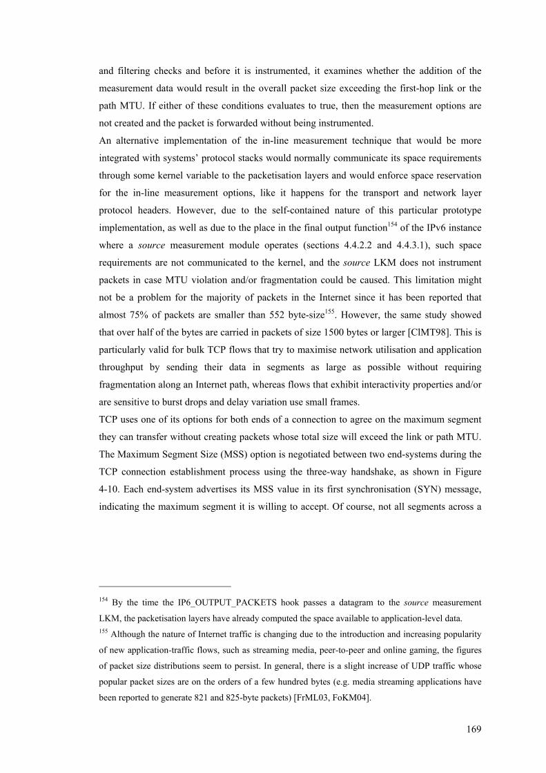
169

and filtering checks and before it is instrumented, it examines whether the addition of the

measurement data would result in the overall packet size exceeding the first-hop link or the

path MTU. If either of these conditions evaluates to true, then the measurement options are

not created and the packet is forwarded without being instrumented.

An alternative implementation of the in-line measurement technique that would be more

integrated with systems’ protocol stacks would normally communicate its space requirements

through some kernel variable to the packetisation layers and would enforce space reservation

for the in-line measurement options, like it happens for the transport and network layer

protocol headers. However, due to the self-contained nature of this particular prototype

implementation, as well as due to the place in the final output function154 of the IPv6 instance

where a source measurement module operates (sections 4.4.2.2 and 4.4.3.1), such space

requirements are not communicated to the kernel, and the source LKM does not instrument

packets in case MTU violation and/or fragmentation could be caused. This limitation might

not be a problem for the majority of packets in the Internet since it has been reported that

almost 75% of packets are smaller than 552 byte-size155. However, the same study showed

that over half of the bytes are carried in packets of size 1500 bytes or larger [ClMT98]. This is

particularly valid for bulk TCP flows that try to maximise network utilisation and application

throughput by sending their data in segments as large as possible without requiring

fragmentation along an Internet path, whereas flows that exhibit interactivity properties and/or

are sensitive to burst drops and delay variation use small frames.

TCP uses one of its options for both ends of a connection to agree on the maximum segment

they can transfer without creating packets whose total size will exceed the link or path MTU.

The Maximum Segment Size (MSS) option is negotiated between two end-systems during the

TCP connection establishment process using the three-way handshake, as shown in Figure

4-10. Each end-system advertises its MSS value in its first synchronisation (SYN) message,

indicating the maximum segment it is willing to accept. Of course, not all segments across a

154 By the time the IP6_OUTPUT_PACKETS hook passes a datagram to the source measurement

LKM, the packetisation layers have already computed the space available to application-level data. 155 Although the nature of Internet traffic is changing due to the introduction and increasing popularity

of new application-traffic flows, such as streaming media, peer-to-peer and online gaming, the figures

of packet size distributions seem to persist. In general, there is a slight increase of UDP traffic whose

popular packet sizes are on the orders of a few hundred bytes (e.g. media streaming applications have

been reported to generate 821 and 825-byte packets) [FrML03, FoKM04].

170

connection have to be of the same size, however, bulk transfer connections will attempt to

perform packetisation to create MSS-sized segments156.

Figure 4-10: Sequence of Messages in TCP three-way Handshake

At the time of development, the advertised MSS of a system was statically computed within

the Linux IPv6 instance to equal the first-hop link MTU (or PMTU157) minus the standard size

of IPv6 and TCP headers. This could prove restrictive for in-line measurement modules

wishing to instrument bulk transfer flows with measurement data, since most of their

segments would be of a prohibitive size. For the purposes of the prototype implementation,

this issue has been circumvented by configuring the source measurement module to decrease

the MSS value advertised in TCP SYN packets, if necessary. If the relevant module parameter

is set, the LKM examines the TCP SYN packets that satisfy the sampling and filtering criteria,

and it replaces the MSS value found in the transport header options field with one that

reserves space for the corresponding in-line measurement header158. This solution obviously

breaks the strict layering of the Internet protocols and would not be advisable for commercial

156 Studies of TCP performance over wide area networks have shown that TCP throughput is directly

proportional to the MSS [MaSM97]. This is one of the reasons for which the increase of the MTU sizes

in the Internet has been suggested. [Math05, Dyks99] 157 During TCP connection establishment the PMTU Discovery process for the corresponding Internet

path might have not been completed. If the PMTU value is available, then it is used to compute the

MSS, since it will always be less than or equal to the first-hop link MTU. 158 A similar mechanism to specify a user-configurable MSS value for TCP connections (mainly to

circumvent PMTU discovery issues) is provided by a Netfilter/iptables module [Hube05]. However, at

the time of development, it was only implemented for the IPv4 instance of the Linux kernel.

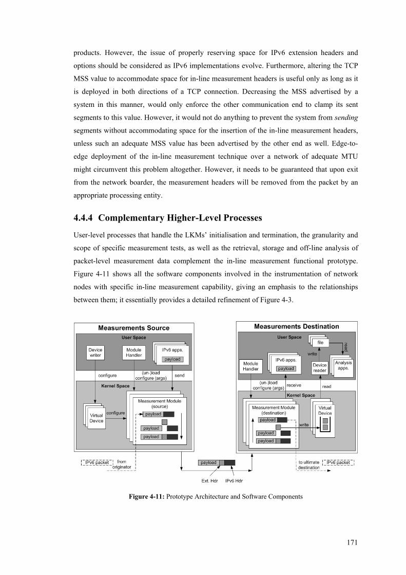
171

products. However, the issue of properly reserving space for IPv6 extension headers and

options should be considered as IPv6 implementations evolve. Furthermore, altering the TCP

MSS value to accommodate space for in-line measurement headers is useful only as long as it

is deployed in both directions of a TCP connection. Decreasing the MSS advertised by a

system in this manner, would only enforce the other communication end to clamp its sent

segments to this value. However, it would not do anything to prevent the system from sending

segments without accommodating space for the insertion of the in-line measurement headers,

unless such an adequate MSS value has been advertised by the other end as well. Edge-to-

edge deployment of the in-line measurement technique over a network of adequate MTU

might circumvent this problem altogether. However, it needs to be guaranteed that upon exit

from the network boarder, the measurement headers will be removed from the packet by an

appropriate processing entity.

4.4.4 Complementary Higher-Level Processes

User-level processes that handle the LKMs’ initialisation and termination, the granularity and

scope of specific measurement tests, as well as the retrieval, storage and off-line analysis of

packet-level measurement data complement the in-line measurement functional prototype.

Figure 4-11 shows all the software components involved in the instrumentation of network

nodes with specific in-line measurement capability, giving an emphasis to the relationships

between them; it essentially provides a detailed refinement of Figure 4-3.

Figure 4-11: Prototype Architecture and Software Components

172

At a node running a source measurement module and performing the actual instrumentation of

traffic with measurement-bearing headers, a handler process which can be as simple as a very

basic shell script, links the appropriate LKM with the running Linux kernel and implicitly

initiates the in-line measurement activity. The module internally maintains a default filtering

and sampling specification which can be overridden with parameters specified by the handler

process during initialisation. During operation, the measurement scope and granularity can be

altered by another user-space process that writes in the virtual character device registered by

the module. This can be a stand-alone process, or an integral part of a more sophisticated

interactive “module-handler” component that will control and dynamically alter the

instrumentation parameters as necessary. The handler can terminate the measurement activity

by removing the source LKM from the running kernel on-demand.

Likewise, the destination module is loaded using a handler process on a node which then

implicitly marks the end of the instrumented path. This is significantly simpler than the

corresponding handler of the source LKM since it does not have to configure any parameters,

upon initialisation or during the module’s operation. The destination LKM performs a direct

measurement observation and amendment only on already instrumented traffic that carries the

appropriate measurement option-bearing header. The LKM can be unloaded by the handler

process, although this is not necessary since the operation of the destination module does not

influence the duration of the measurement activity. In other words, it can be an always-on

measurement module that examines incoming traffic, and in the presence of appropriately-

instrumented (by a corresponding source module) datagrams it performs the relevant actions;

otherwise it returns the packets un-changed in the networking stack. Such operation of course

incurs an overhead of always examining whether incoming packets contain any in-line

measurement headers. However, similar simple tests are also performed by the core of the

networking stack to examine if, for example, an IPv6 datagram carries any extension headers.

The most important user-space components coupled with the operation of a destination in-line

measurement LKM are the processes that read the kernel module’s two-point measurement-

related data back into user-space, write it out to a file in a suitable format and then post-

process and analyse the results to implement either simple or derived aggregate performance

metrics for the instrumented IPv6 flows of interest. A process operating in real-time, extracts

the per-packet header data by issuing read IOCTL calls on the module’s registered virtual

device, each of which returns the oldest element from the destination LKM’s FIFO queue.

This operation can be implemented either wholly in a language that allows direct access to the

native environment, or by using a native interface of a language which presents a more

restricted abstraction of that environment. For each packet, the extracted sequence of bytes is

then parsed by protocol decoders which identify the specific network and transport layer

headers and the type of the deployed in-line measurement, and subsequently, a subset of these

173

protocol fields are written to local files. The amount of data actually stored on disk depends

on the type of post-analysis, however, there are some control fields that can be omitted and

partial byte capture can be further increased. For example, even if post-processing requires

network and transport header fields in conjunction with the in-line measurement indicators to

provide for more sophisticated and synthetic performance analysis, protocol fields such as the

network layer’s version number, Next Header, Opt Data Len, as well as TCP’s checksum and

most of the flags will rarely be needed159.

Further analysis applications that complete the in-line measurement prototype are transport-

protocol-specific and operate off-line by reading the data stored during the instrumentation

process and implementing a variety of performance metrics based on the per-packet

measurement indicators. Unidirectional transport-layer flows are reconstructed based on the

stored header fields, and numerous characteristics of the flows are computed, both on a per-

packet and on a cumulative per-flow basis.

Figure 4-11 also shows the interaction of the prototype with existing IPv6 applications

interpedently sending and receiving their payload data, which is then instrumented with the in-

line measurement header options. The figure emphasises the case where the measurement

modules are instantiated on the true end-points of a unidirectional end-to-end Internet path,

and hence shows instrumentation taking place between the actual originator and destination of

the IPv6 traffic. However, the dashed lines also illustrate the case where the measurement

source and destination modules reside on intermediate nodes of an end-to-end path and are

instrumenting traffic to be further forwarded, rather than traffic originating or delivered

locally. In order to maintain the simplicity of the diagram, packets are shown to arrive at the

measurement module from the network and then being forwarded after instrumentation has

taken place. Of course, in reality, packets go through the normal processing routines of the

systems’ IPv6 instance, before they are passed to the loaded measurement modules’ code.

After instrumentation has completed, datagrams are passed again to IPv6 routines that forward

them towards a remote host (Figure 4-6).

159 For example, for the purposes of this prototype, out of the total 84 bytes (40 + 24 + 20) occupied by

the IPv6, OWD option-bearing extension header and TCP header, only 66 bytes need to be stored on

disk. These are accumulated by the IPv6 source and destination addresses, IPv6 payload length, OWD

source and destination timestamps, TCP sequence number, acknowledgment, source and destination

ports, data offset, TCP flags and window fields.

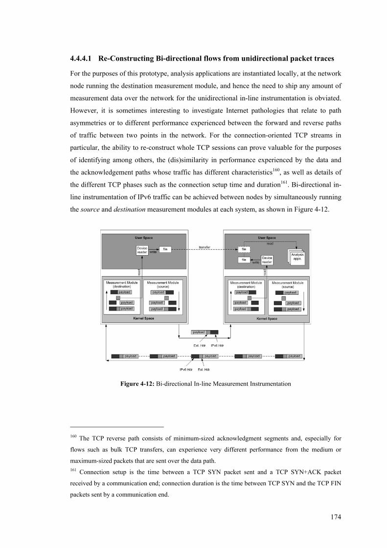
174

4.4.4.1 Re-Constructing Bi-directional flows from unidirectional packet traces

For the purposes of this prototype, analysis applications are instantiated locally, at the network

node running the destination measurement module, and hence the need to ship any amount of

measurement data over the network for the unidirectional in-line instrumentation is obviated.

However, it is sometimes interesting to investigate Internet pathologies that relate to path

asymmetries or to different performance experienced between the forward and reverse paths

of traffic between two points in the network. For the connection-oriented TCP streams in

particular, the ability to re-construct whole TCP sessions can prove valuable for the purposes

of identifying among others, the (dis)similarity in performance experienced by the data and

the acknowledgement paths whose traffic has different characteristics160, as well as details of

the different TCP phases such as the connection setup time and duration161. Bi-directional in-

line instrumentation of IPv6 traffic can be achieved between nodes by simultaneously running

the source and destination measurement modules at each system, as shown in Figure 4-12.

Figure 4-12: Bi-directional In-line Measurement Instrumentation

160 The TCP reverse path consists of minimum-sized acknowledgment segments and, especially for

flows such as bulk TCP transfers, can experience very different performance from the medium or

maximum-sized packets that are sent over the data path. 161 Connection setup is the time between a TCP SYN packet sent and a TCP SYN+ACK packet

received by a communication end; connection duration is the time between TCP SYN and the TCP FIN

packets sent by a communication end.

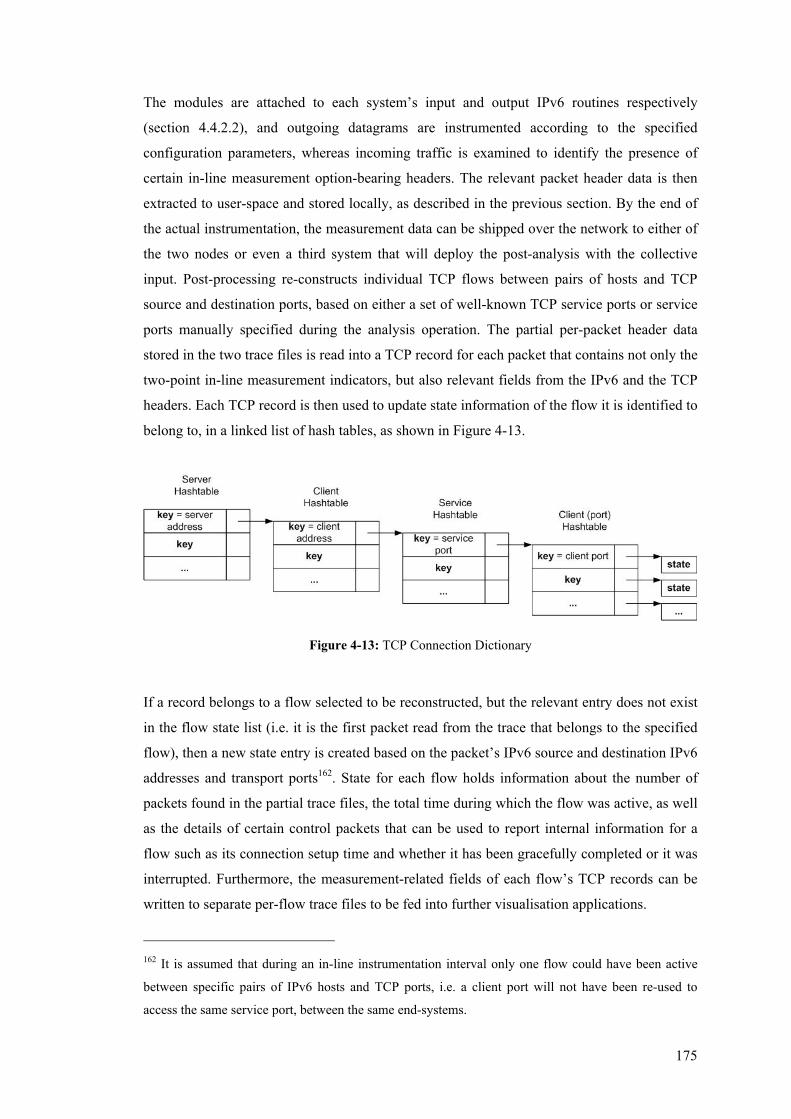
175

The modules are attached to each system’s input and output IPv6 routines respectively

(section 4.4.2.2), and outgoing datagrams are instrumented according to the specified

configuration parameters, whereas incoming traffic is examined to identify the presence of

certain in-line measurement option-bearing headers. The relevant packet header data is then

extracted to user-space and stored locally, as described in the previous section. By the end of

the actual instrumentation, the measurement data can be shipped over the network to either of

the two nodes or even a third system that will deploy the post-analysis with the collective

input. Post-processing re-constructs individual TCP flows between pairs of hosts and TCP

source and destination ports, based on either a set of well-known TCP service ports or service

ports manually specified during the analysis operation. The partial per-packet header data

stored in the two trace files is read into a TCP record for each packet that contains not only the

two-point in-line measurement indicators, but also relevant fields from the IPv6 and the TCP

headers. Each TCP record is then used to update state information of the flow it is identified to

belong to, in a linked list of hash tables, as shown in Figure 4-13.

Figure 4-13: TCP Connection Dictionary

If a record belongs to a flow selected to be reconstructed, but the relevant entry does not exist

in the flow state list (i.e. it is the first packet read from the trace that belongs to the specified

flow), then a new state entry is created based on the packet’s IPv6 source and destination IPv6

addresses and transport ports162. State for each flow holds information about the number of

packets found in the partial trace files, the total time during which the flow was active, as well

as the details of certain control packets that can be used to report internal information for a

flow such as its connection setup time and whether it has been gracefully completed or it was

interrupted. Furthermore, the measurement-related fields of each flow’s TCP records can be

written to separate per-flow trace files to be fed into further visualisation applications.

162 It is assumed that during an in-line instrumentation interval only one flow could have been active

between specific pairs of IPv6 hosts and TCP ports, i.e. a client port will not have been re-used to

access the same service port, between the same end-systems.

176

4.5 Summary The implementation details of a prototype system that facilitates IPv6-based in-line

measurement between two points in the network have been presented in this chapter. By

adopting a highly modular design that lends itself well to a distributed measurement

framework, the different realisation alternatives of the core measurement components as

hardware, software or hybrid modules have been briefly discussed.

The selection of Linux as a platform to build the software-based in-line measurement

prototype has been elaborated, and the operational design choices and implementation details

of the prototype have been thoroughly discussed. Different actions are performed by the in-

line measurement Loadable Kernel Modules (LKM)s, depending not only on the type of

measurement they perform, but also on whether they operate at the source or at the destination

of a unidirectional instrumented path.

Partial byte capture, packet filtering, and packet sampling are three distinct mechanisms that

have been employed by the prototype to provide for configurable levels of scope and

granularity and reduce the cost associated with the measurement process. In addition, enabling

the instrumentation of connection-oriented flows that consist of maximum-sized datagrams

has been taken into consideration and addressed through appropriate adjustment of the

maximum transport layer Payload Data Unit (PDU).

Finally, the deployment and operation of user-space processes that complement the prototype

by enabling the initialisation and handling of the core measurement components, as well as by

synthesising raw, per-packet measurement data to implement a variety of performance

metrics, have been presented.

177

Chapter 5

5Instrumenting IPv6

Application Flows 5.1 Overview An evaluation of the in-line measurement technique is presented in this chapter through the

instrumentation of representative IPv6 application flows over different-capacity operational

topologies. Native and tunnelled end-to-end IPv6 experiments over the Internet have been

facilitated by the Mobile-IPv6 Systems Research Laboratory (MSRL) infrastructure whose

topology and connectivity are described in the following sections. Representative performance

metrics are implemented and presented to reveal numerous properties of interest for a diverse

set of instrumented flows. Experiments are decomposed down to two categories instrumenting

TCP and UDP flows, respectively. For each transport-based category the One-Way Delay

(OWD) IPv6 measurement destination option is used to implement a set of time-related

performance metrics, and the One-Way Loss (OWL) IPv6 measurement destination option to

provide insight on unidirectional packet loss phenomena, such as dropped and retransmitted

packets, as well as packets delivered out of order to the destination. Time synchronisation

issues, as well as tactics to improve system clock accuracy over high-capacity paths are also

briefly discussed. The overhead associated with the in-line measurement technique is

evaluated, and two systematic sampling schemes are used to indicatively demonstrate the

potential greater overhead reduction, together with its consequential influence in measurement

accuracy due to the reduction of the sample space. Finally, the in-line measurement technique

is compared to complementary measurement techniques and tools through both a quantitative

analysis, and a qualitative discussion that concludes this chapter.

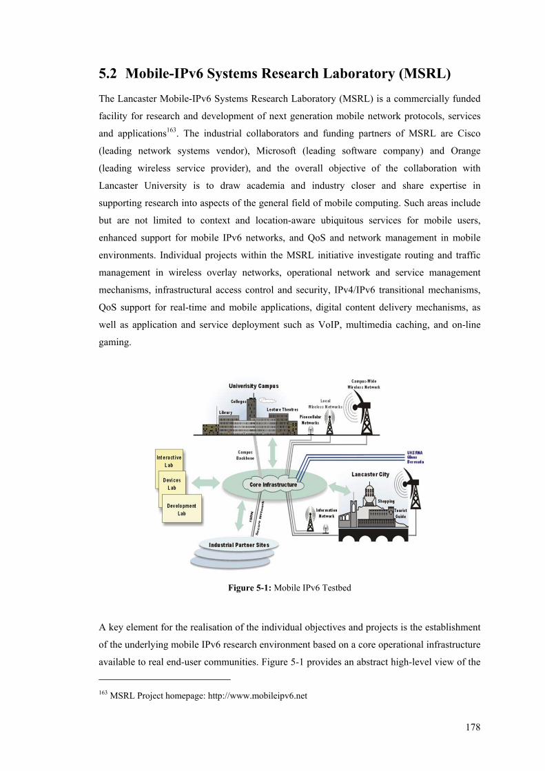
178

5.2 Mobile-IPv6 Systems Research Laboratory (MSRL) The Lancaster Mobile-IPv6 Systems Research Laboratory (MSRL) is a commercially funded

facility for research and development of next generation mobile network protocols, services

and applications163. The industrial collaborators and funding partners of MSRL are Cisco

(leading network systems vendor), Microsoft (leading software company) and Orange

(leading wireless service provider), and the overall objective of the collaboration with

Lancaster University is to draw academia and industry closer and share expertise in

supporting research into aspects of the general field of mobile computing. Such areas include

but are not limited to context and location-aware ubiquitous services for mobile users,

enhanced support for mobile IPv6 networks, and QoS and network management in mobile

environments. Individual projects within the MSRL initiative investigate routing and traffic

management in wireless overlay networks, operational network and service management

mechanisms, infrastructural access control and security, IPv4/IPv6 transitional mechanisms,

QoS support for real-time and mobile applications, digital content delivery mechanisms, as

well as application and service deployment such as VoIP, multimedia caching, and on-line

gaming.

Figure 5-1: Mobile IPv6 Testbed

A key element for the realisation of the individual objectives and projects is the establishment

of the underlying mobile IPv6 research environment based on a core operational infrastructure

available to real end-user communities. Figure 5-1 provides an abstract high-level view of the

163 MSRL Project homepage: http://www.mobileipv6.net

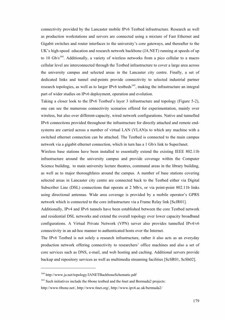
179

connectivity provided by the Lancaster mobile IPv6 Testbed infrastructure. Research as well

as production workstations and servers are connected using a mixture of Fast Ethernet and

Gigabit switches and router interfaces to the university’s core gateways, and thereafter to the

UK’s high-speed education and research network backbone (JA.NET) running at speeds of up

to 10 Gb/s164. Additionally, a variety of wireless networks from a pico cellular to a macro

cellular level are interconnected through the Testbed infrastructure to cover a large area across

the university campus and selected areas in the Lancaster city centre. Finally, a set of

dedicated links and tunnel end-points provide connectivity to selected industrial partner

research topologies, as well as to larger IPv6 testbeds165, making the infrastructure an integral

part of wider studies on IPv6 deployment, operation and evolution.

Taking a closer look to the IPv6 Testbed’s layer 3 infrastructure and topology (Figure 5-2),

one can see the numerous connectivity scenarios offered for experimentation, mainly over

wireless, but also over different-capacity, wired network configurations. Native and tunnelled

IPv6 connections provided throughout the infrastructure for directly attached and remote end-

systems are carried across a number of virtual LAN (VLAN)s to which any machine with a

switched ethernet connection can be attached. The Testbed is connected to the main campus

network via a gigabit ethernet connection, which in turn has a 1 Gb/s link to SuperJanet.

Wireless base stations have been installed to essentially extend the existing IEEE 802.11b

infrastructure around the university campus and provide coverage within the Computer

Science building, to main university lecture theatres, communal areas in the library building,

as well as to major thoroughfares around the campus. A number of base stations covering

selected areas in Lancaster city centre are connected back to the Testbed either via Digital

Subscriber Line (DSL) connections that operate at 2 Mb/s, or via point-point 802.11b links

using directional antennas. Wide area coverage is provided by a mobile operator’s GPRS

network which is connected to the core infrastructure via a Frame Relay link [ScJR01].

Additionally, IPv4 and IPv6 tunnels have been established between the core Testbed network

and residential DSL networks and extend the overall topology over lower capacity broadband

configurations. A Virtual Private Network (VPN) server also provides tunnelled IPv4/v6

connectivity in an ad-hoc manner to authenticated hosts over the Internet.

The IPv6 Testbed is not solely a research infrastructure, rather it also acts as an everyday

production network offering connectivity to researchers’ office machines and also a set of

core services such as DNS, e-mail, and web hosting and caching. Additional servers provide

backup and repository services as well as multimedia streaming facilities [ScSR01, ScSh02].

164 http://www.ja.net/topology/JANETBackboneSchematic.pdf 165 Such initiatives include the 6bone testbed and the 6net and Bermuda2 projects:

http://www.6bone.net/, http://www.6net.org/, http://www.ipv6.ac.uk/bermuda2/

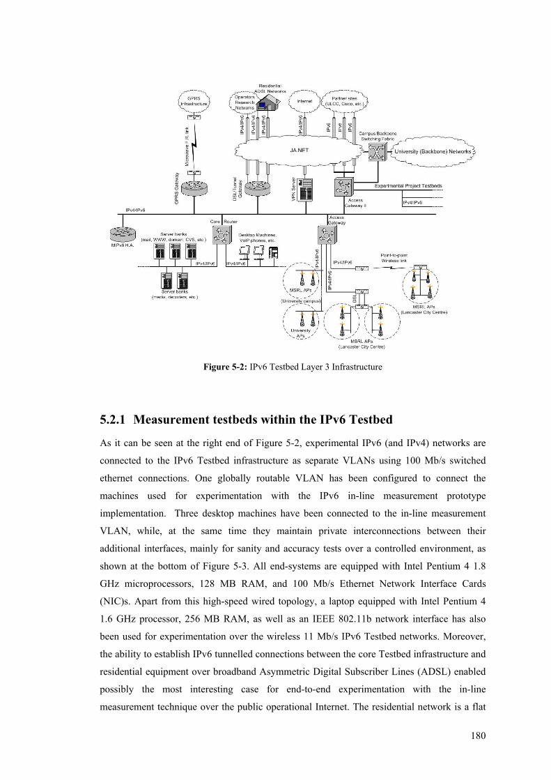
180

Figure 5-2: IPv6 Testbed Layer 3 Infrastructure

5.2.1 Measurement testbeds within the IPv6 Testbed

As it can be seen at the right end of Figure 5-2, experimental IPv6 (and IPv4) networks are

connected to the IPv6 Testbed infrastructure as separate VLANs using 100 Mb/s switched

ethernet connections. One globally routable VLAN has been configured to connect the

machines used for experimentation with the IPv6 in-line measurement prototype

implementation. Three desktop machines have been connected to the in-line measurement

VLAN, while, at the same time they maintain private interconnections between their

additional interfaces, mainly for sanity and accuracy tests over a controlled environment, as

shown at the bottom of Figure 5-3. All end-systems are equipped with Intel Pentium 4 1.8

GHz microprocessors, 128 MB RAM, and 100 Mb/s Ethernet Network Interface Cards

(NIC)s. Apart from this high-speed wired topology, a laptop equipped with Intel Pentium 4

1.6 GHz processor, 256 MB RAM, as well as an IEEE 802.11b network interface has also

been used for experimentation over the wireless 11 Mb/s IPv6 Testbed networks. Moreover,

the ability to establish IPv6 tunnelled connections between the core Testbed infrastructure and

residential equipment over broadband Asymmetric Digital Subscriber Lines (ADSL) enabled

possibly the most interesting case for end-to-end experimentation with the in-line

measurement technique over the public operational Internet. The residential network is a flat

181

100 Mb/s topology which also includes an IEEE 802.11b station offering wireless

connectivity, while the ADSL gateway (Cisco C827 processor) is equipped with an ATM and

a 10 Mb/s Ethernet interfaces. The main instrumented end-system within this simple network

configuration is equipped with an Intel Celeron 1 GHz processor and 256 MB RAM.

Figure 5-3: Measurement Testbeds within the MSRL Infrastructure

All five end-systems used for the in-line IPv6 measurement experiments run Linux kernel

versions 2.4.18 and 2.4.19 and have been instrumented with the kernel hooks as well as the

source and destination One-Way Delay (OWD) and One-Way Loss (OWL) Loadable Kernel

Modules (LKM)s, as documented in sections 4.4.2.2 and 4.4.3. Each system can run a

number of the measurement LKMs in parallel to instrument outgoing traffic according to a

defined filtering and sampling specification (section 4.4.3.6), or to perform a direct

measurement observation to appropriately instrumented incoming traffic, or both. Depending

on the LKMs loaded at any time, a given system implicitly marks the source or/and the

destination of an instrumented IPv6 path. As it can be seen from Figure 5-3, sets of two-point

in-line measurement experiments can be conducted end-to-end over three different-capacity

paths, by enabling measurement LKMs to instrument traffic flows initiated at and exchanged

between two given systems of the in-line measurement testbed.

End-systems directly attached to the 100 Mb/s switched ethernet VLAN provide for a less

interesting experimentation scenario, due to the high-speed topology and configuration which

avoids sources of network delay. All three systems connect to a gigabit switch which only

182

provides connectivity to experimental VLANs as opposed to large, continuously-used

production environments. Hence, this wired topology can be considered as over-provisioned

for the purposes of two-point internal experiments (i.e. between hosts directly attached to the

gigabit switch) whose 100 Mb/s narrow links166 are interconnected via a gigabit backplane

switch. Within such an environment, the time to transfer a maximum-sized 1500-byte

datagram between two hosts can be as little as 0.12 milliseconds (120 µs), and moreover the

time to transfer a minimum-sized 60-byte datagram167 can be around 0.0048 milliseconds (4.8

µs). The same holds also true for the private 100 Mb/s networks interconnecting the three end-

systems, and it is therefore clear that there is space for undetectable and non-negligible

measurement errors and inaccuracies over these high-speed networks, especially for a non-

hardware-assisted prototype system running on commodity PC configurations. The two main

sources of measurement errors relate to the system processing overhead and the software-

based time synchronisation mechanisms. As it has been briefly raised in section 4.4.3.5, a

user-space process that would read per-packet measurement data from the corresponding

LKM’s queue at 100 Mb/s full line speed would need to make a reading every few

microseconds in order for the queue buffer not to overflow, a resolution that might simply not

be achievable due to context switching and Operating System (OS) scheduling priorities.

Consequently, measurement data can be dropped and, especially for two-point loss and inter-

packet measurements, produce misleading results for the phenomenon of interest. In addition,

it is envisaged that IPv6 in-line measurements can be implemented not only at intermediate

network nodes using hardware-assisted optimisation techniques, but also at commodity end-

systems as an integrated software tool (similar to, for example, today’s ping

implementations) that can be used to assess the performance properties of application flows,

and consequently, the prototype implementation and the measurement testbeds have been

realised and configured using general-purpose end-system configurations. Therefore, the

instrumented systems used the Network Time Protocol (NTP) [Mill91] to synchronise their

local clocks in order to produce two-point time-related measurements, as opposed to

customised reference clocks such as, for example, Global Positioning System (GPS) receivers.

NTP has been reported to provide synchronisation accuracy in the range of a millisecond or

two in LANs and up to few tens of milliseconds in global WANs [Ntp05]. It is therefore

evident that in an environment where the actual latencies can be in the range of even a few

hundreds of microseconds, the measurement error might well be greater than the actual

observed phenomenon. Indeed, typical figures of average Round-Trip-Time (RTT) measured

166 Narrow link is the slowest forwarding element that determines the (end-to-end) capacity of a path,

according to the bandwidth estimation-related definition (section 2.2.6). 167 Such as, for example, a TCP acknowledgment segment over IPv6.

183

by ping (64-byte ICMP datagrams) between the 100 Mb/s ethernet-connected systems vary

from 0.3 to 0.5 milliseconds.

On the other hand, experiments over the IPv6 Testbed wireless networks can prove more

interesting, both due to the relatively lower capacity of the medium168, but also due to the

operational nature of the wireless topologies, which constitutes the presence of competing

traffic almost certain. The 11 Mb/s wireless link can in theory transfer a 1500-byte datagram

in 1.09 milliseconds and a 60-byte datagram in 0.0436 milliseconds (43,6 µs), however, traffic

between a wireless node and an end-system attached to the wired in-line measurement VLAN

traverses a 3-hop path with significantly more sources of network delays, including the layer-

3 network nodes, the wireless access points (bridges) as well as the additional cross-traffic.

During a quiet period, the RTT measured by ping (64-byte ICMP datagrams) between a

wireless station and a host attached to the in-line measurement VLAN varied from 1.8 to 3.5

milliseconds.

The most interesting experimentation scenario is undoubtedly over the tunnelled IPv6 links

that connect the residential network to the IPv6 Testbed core, over an ADSL connection.

Traffic between hosts attached to the 100 Mb/s VLAN and the instrumented systems of the

residential network is transferred over a global WAN which typically involves a 13-hop

operational Internet path. Assuming the narrow link is the asymmetric 512/256 kb/s ADSL

access line (50:1 contention) which determines the end-to-end capacity of the path, then in

theory this link can receive a 1500-byte datagram in 23.4 milliseconds and a 60-byte datagram

in 0.938 milliseconds, whereas the corresponding transmit times are twice as long. However,

the sources of network delay are multiple and the competing traffic is certainly almost always

present, resulting in a typical average RTT between 45 and 48 milliseconds for traffic between

the residential network and the IPv6 Testbed core, as this is measured by ping (64-byte ICMP

datagrams) while little or no competing traffic is present at the edges of the end-to-end path.

5.3 Implementing Representative Performance Metrics Internet traffic can be decomposed down to two broad categories, based on the end-to-end

transport service that provides the communication between the application end-points at the

distant systems, and handles packetisation of the data stream that is then routed and delivered

by the Internet Protocol mechanisms [Come00]. As it has been reported in earlier studies and

briefly discussed in section 2.3.3.4, the vast majority of the traffic mix is handled either by the

connectionless datagram delivery service (UDP) or by the reliable stream transport service

(TCP), and only a small fraction of control traffic is attributed to different protocols, such as, 168 The capacity of the narrow (wireless) link can vary depending on the physical position of the

wireless node (end-system).

184

for example ICMP and routing protocols [ClMT98]. Applications choose between the two

main transport mechanisms depending on their performance requirements and their

consequential sensitivity to different factors of performance degradation. Hence, TCP is

preferred for applications whose primary requirement is the reliable and optimal delivery of

data, whereas UDP is mainly used by applications which are far more sensitive to timely and

continuous delivery of data than in occasional data loss. TCP has traditionally been the

dominant protocol for data transport and the dramatic explosion of the World Wide Web

(WWW) has resulted in TCP carrying the vast majority of packets, bytes and flows over the

Internet. UDP has been suggested as a transport mechanism for real-time and networked

multimedia applications169, as well as for applications that only occasionally exchange a very

small amount of messages for which the overhead of connection establishment is considered

unjustifiably high, such as Domain Name System (DNS) and NTP queries.

The IPv6 in-line measurement source and destination modules together with the user-level

analysis processes have been used to directly implement a set of (empirically-specified) two-

point unidirectional simple and derived performance metrics170 of interest for application

flows using each of the two main Internet transport mechanisms. Time-related metrics have

been implemented based on timestamp indicators carried within the OWD TLV-encoded

option (section 3.8.1) and datagram loss-related measures have been computed based on the

IPv6-layer sequence indicators carried within the OWL TLV-encoded option (section 3.8.2).

Arguably one of the most important and well-studied metrics for a TCP connection is the

throughput achieved by the protocol’s congestion avoidance algorithm and its different

implementations and/or extensions171. The throughput of a TCP connection can be limited by

a number of factors, including the receiver’s advertised window, the total transfer size, the

path RTT, the probability of random losses, as well as the available bandwidth in the forward

and reverse paths [JaDo02]. When a connection is only limited by the network and not by

end-host constraints this metric can also be called Bulk Transfer Capacity (BTC), in relation

to MaAl01 (discussed in section 2.2.2). Throughput has been defined in the past both in terms

of bytes and in terms of packets sent over a given time interval. In this thesis, the throughput

of a bulk transfer TCP connection/flow is defined in terms of bytes. Considering a TCP flow

169 Advances in multimedia streaming are also considering TCP as a transport mechanism over the

Internet, especially for low bit-rate streams. 170 In accordance to the definitions provided in sections 2.2.1 and 3.7.1. 171 TCP throughput has mainly been measured and modelled in the literature for bulk transfer TCP

flows, which in theory are flows with an unlimited amount of data to send. In practice, a bulk transfer

TCP flow is a flow with a large amount of data to send such as, for example, FTP transfers. Example

studies on TCP throughput include [MaSM97, PaFT98] and references therein.

185

starting at time 0t and ending at time 0ft t> , for any given time interval 00 , ft t t > ∈ , stB

is defined to be the number of bytes sent during the time interval t . Then the throughput tT for

this time interval is defined as:

st

tBTt

= (8)

Since in practice the TCP throughput is usually measured and averaged over the entire bulk

transfer time, then the overall throughput T of the TCP connection that has sent a total of sB

number of bytes is computed as:

0

s

f

BTt t

=−

(9)

Throughput accounts for the number of bytes sent per unit of time regardless of their eventual

fate172 [PaFT98]. In-line measurements being a receiver-based measurement technique173, is

able to measure the goodput G of a TCP connection as the number of bytes rB received over

the time interval between 0 0t t′ > (being the time the first datagram arrived at the receiver)

and 0ft t′ ′> (the time the last datagram arrived at the receiver):

0

r

f

BGt t

=′ ′−

(10)

Accordingly, for a given time interval 00 [ , ]ft t t′ ′′ > ∈ during which rtB ′ number of bytes has

reached the receiver of the TCP connection, the goodput tG ′ for this interval is defined as:

rt

tBGt′

′ = ′ (11)

It is evident that both throughput and goodput are single-point metrics implemented at the

sender and the receiver of a TCP connection respectively, and consequently mask out the

component of the end-to-end path one-way delay experienced by individual datagrams. Both

metrics are concerned with aggregate measures within a flow, averaged over a significant

elapsed time. At the same time, although the in-line measurement enables the instrumentation

of particular transport flows and can compute aggregate representative performance metrics,

the technique operates at the network layer between two Internet points and hence has an

intrinsic interest in the per-packet dynamics while these are routed from the source to the

172 Datagrams carrying a given number of bytes sent by the sender might be dropped (lost) along the

path and never reach the receiver. 173 The direct measurement observation takes place at the destination LKM.

186

destination of an instrumented path. An interesting metric that can be facilitated by the in-line

measurement techniques and directly relates to the performance of a transport (e.g. TCP) flow

is the IPv6 per-packet data transfer rate. For any given IPv6 packet p of a packet data size

pS (as indicated by the Payload Length field of the IPv6 header, excluding any IPv6 header

bytes) sent from the sender at time st and arriving at the receiver at time rt , with r st t> , the

data transfer rate R for p is defined as follows:

p

r s

SR

t t=

− (12)

Irrespective of transport protocol, another per-packet property that has been well-studied and

modelled in the past is the packet inter-arrival time. For any two successive packets i and j

( 1j i− = ) arriving at the receiver at times rit and r

jt respectively, the packet inter-arrival

time ( , )i jIA is defined as:

( , )r r

i j j iIA t t= − (13)

The two-point nature of the in-line measurement also facilitates the implementation of packet

inter-departure time ( ( , )i jID ) from a sender in a similar fashion, for two consecutive packets

departing at times sit and s

jt , respectively.

( , )s s

i j j iID t t= − (14)

Packet inter-arrival times computed over the duration of a connection can be used to

approximate the goodput of the connection174. TCP mainly sends data in bursts until reaching

a number of unacknowledged bytes equal to the minimum of the congestion and receiver

windows, and the inter-arrival time between two consecutive packets can be seen as the time

taken for a certain number of bytes (packet size) to arrive at the receiver of the TCP

connection. Again, the actual time to transfer a packet from the sender to the receiver is

masked out and no assumptions are made about the rate at which the sender transmits packets.

For a flow of n consecutive packets, each transferring ib bytes and arriving at the receiver at

time rit , the average goodput G of that flow can be approximated as follows:

174 Similarly, packet inter-departure times can be used to estimate the throughput of a connection.

However, using the receiver-based in-line measurement technique, inter-departure times are computed

only for packets that actually arrived at the receiver, and can be used in comparison to the inter-arrival

time for any given pair of consecutive packets to estimate the effect of network delay.

187

11

1 1

1

ni

r ri i i

bt tGn

−+

= + −≈

−

∑ (15)

Multimedia streaming and online gaming, two of the major applications of UDP traffic,

although they can share some common generic requirements with other application flows,

have a number of specific requirements mainly regarding the real-time transmission of

continuous media information. Hence, while UDP traffic might also be concerned with the

achievable throughput for a flow, the intrinsic interest is in the performance properties of the

individual datagrams, rather than on aggregate quantities concerning the flow as a whole. The

end-to-end one-way delay experienced by each UDP datagram, as well as the variation of the

delay over time are two major factors influencing the performance of UDP applications. Delay

variation for example is very important especially for real-time sound, since it influences both

the overall delay of an application, and the buffering requirements of the receiving system

[Fluc95]. Not only for streaming applications, but even for network time synchronisation

(NTP), the network latency experienced is considered the most important parameter for the

process’ accuracy and smooth operation. The end-to-end one-way delay experienced by any

given packet i departed at time sit from the sender and arrived at time r

it at the receiver is

computed as:

r si i iD t t= − (16)

The delay variation or jitter between two successive packets i and j ( 1j i− = )

experiencing delays and i jD D , respectively, is implemented as:

( , )i j j iJ D D= − (17)

Depending on the values jitter assumes based on Equation 17, the trend of the one-way delay

can be revealed. Positive values show an increase in the one-way delay and negative values

show a decrease. Depending on the persistence of the observed trend in time, as well as on the

absolute values jitter takes, one can make observations about the network’s performance. For

example, a steadily increasing trend reaching a mode, and then followed by a decreasing

trend, can be associated with a network saturation phenomenon that reached a peak and then

(for some reason) normal-load operation has been restored. Another interesting property of

jitter is that while one-way delay is sensitive to and assumes clock synchronisation between

the two instrumented systems where the measurement takes place, its variation (jitter) is not.

This can be seen mainly by substituting equation 16 to equation 17:

( , ) ( , ) ( , )( ) ( ) ( ) ( )r s r s r r s si j j i j j i i j i j i i j i jJ D D t t t t t t t t IA ID= − = − − − = − − − = − (18)

Apart from the numerous time-related metrics implemented using the in-line OWD option for

the different transport flows according to their interests in different performance indicators,

188

packet loss has been implemented and measured for both reliable and unreliable transports.

Packet loss can influence diverse flows in different ways. For example, loss phenomena can

result in discontinuity of a streaming media UDP session, and the degrading of the

performance of a TCP connection through longer elapsed time. Using the OWL source

measurement module to insert IPv6-layer sequence numbers to outgoing packets as described

in section 4.4.3.4, the instantaneous packet loss ( , )i jL between two successively received

packets i and j ( 1j i− = ) at the destination of an instrumented path with network-level

(IPv6) sequence numbers and i jSeq Seq , respectively, is computed as follows:

( , ) ( ) 1i j j iL Seq Seq= − − (19)

5.4 TCP Measurements Two broad sets of measurements have been conducted using the IPv6 in-line measurement

prototype implementation, in order to demonstrate their ability to potentially instrument any

type of traffic routed and delivered by the next generation Internet Protocol. The first set of

measurements mainly concentrate on revealing certain performance aspects of bulk transfer

TCP connections, and the second set measures the performance experienced by UDP video

streaming traffic. Both TCP and UDP measurements have been realised using the

measurement indicators carried within the OWD and OWL IPv6 destination options to

implement selected representative performance metrics as outlined in the previous section,

mainly over wireless and ADSL instrumented paths. Measurements have been conducted end-

to-end by instrumenting the ultimate source and destination nodes of a path with the

appropriate measurement LKMs. Then, user-space client/server processes initiated the

corresponding traffic exchange and the generated IPv6 datagrams have been instrumented

‘on-the-fly’ with the relevant measurement indicators.

The reason for this decomposition of measurement experiments down to two separate sets is

mainly twofold. First, it has been decided to implement different performance metrics for the

two different transport mechanisms that would best describe the requirements of the selected

applications. At the same time, this also demonstrates the broad applicability of the in-line

measurement technique to provide for a generic instrumentation mechanism for the IPv6

Internet. And second, the actual instrumentation for TCP connections and for the

connectionless UDP datagram delivery mechanism is slightly different. In the simplest case of

instrumenting an end-to-end unidirectional UDP flow, it is only required to load a source

measurement module at the originator of the traffic flow and a destination measurement

module at the receiver, as this process has been described in section 4.4 and shown in Figure

4-3. On the other hand, producing an overall instrumentation for a full-duplex TCP connection

189

requires the simultaneous operation of a source and a destination measurement module at both

communication end-systems, as well as the collective processing of the measurement data for

the identification and reconstruction of the bi-directional flow. This process has been

described in section 4.4.4.1.

TCP has been and remains the dominant transport protocol carrying the vast majority of all

traffic over the Internet for a variety of applications, ranging from interactive sessions such as

SSH and telnet, to short-lived flows (e.g. HTTP) and long-lived bulk data transfers. The in-

line measurement modules have been used to instrument TCP file transfers (FTP) of relatively

small-sized data files of approximately 6 MB (6154240 bytes). This choice has been made in

order to obviate the need to simulate end-user behaviour which would influence the burstiness

of the traffic and consequently the perceived performance in the case, for example, of an

interactive or a Web-TCP session. Rather, a file transfer is handled solely by the end-systems’

TCP implementations, and the perceived performance is influenced purely by network

topology and load. The file size was chosen to be moderate so that it results in a few thousand

lines of trace files, while at the same time it approximates the size of a compressed digital

audio file, a very common type of file exchanged over today’s increasingly popular peer-to-

peer overlay topologies. In addition, such File Transfer Protocol (FTP) session can resemble a

bulk transfer TCP connection as defined in MaAl01, offering a significant quantity of bytes to

be exchanged between the two communication ends. The time to transfer such data file can

normally vary from a few seconds over a high-speed LAN connection to a few minutes over a

broadband WAN connection.

In order to demonstrate the transparency and the inter-operation of the in-line measurement

prototype implementation with current general-purpose system software and user-space

processes (sections 3.7 and 4.1), existing Off The Shelf (OTS) applications were chosen to

generate the traffic flows that would then be instrumented by the loaded measurement

modules. Pure-FTPd (version 1.0.12) is a secure production-quality and standard-conformant

FTP server that has been used for the bulk transfer TCP experiments between two

instrumented systems over the wireless and ADSL IPv6 paths. Pure-FTPd has been among the

first standalone FTP servers to incorporate full IPv6 support, and is currently used by a

number of highly loaded production servers as well as on embedded systems [Pure].

All instrumented systems implement TCP according to the protocol specification standard

[Post81b], incorporating the communications protocol layers’ requirements for Internet hosts

software [Brad89], and the TCP slow start, congestion avoidance, fast retransmit and fast

recovery algorithms [Stev97]. The NewReno modification to TCP fast recovery algorithm

[FlHe99] and Selected Acknowledgment (SACK) extensions [MaMF96] are also included in

the protocol implementations.

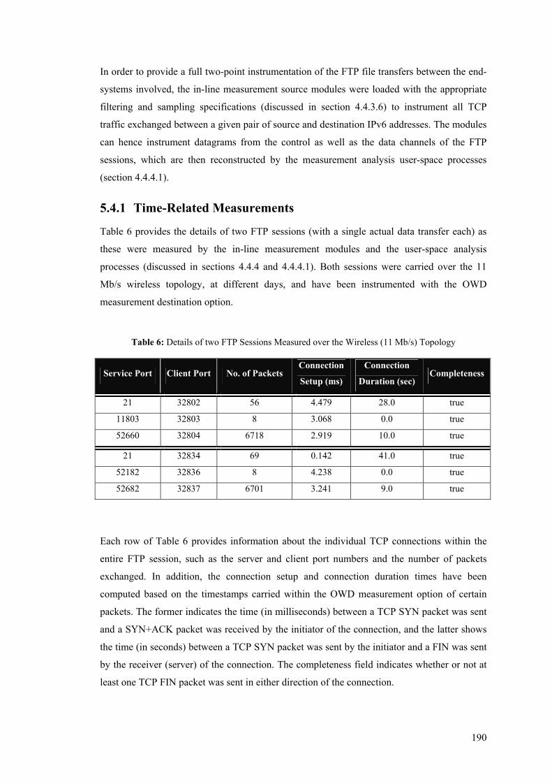
190

In order to provide a full two-point instrumentation of the FTP file transfers between the end-

systems involved, the in-line measurement source modules were loaded with the appropriate

filtering and sampling specifications (discussed in section 4.4.3.6) to instrument all TCP

traffic exchanged between a given pair of source and destination IPv6 addresses. The modules

can hence instrument datagrams from the control as well as the data channels of the FTP

sessions, which are then reconstructed by the measurement analysis user-space processes

(section 4.4.4.1).

5.4.1 Time-Related Measurements

Table 6 provides the details of two FTP sessions (with a single actual data transfer each) as

these were measured by the in-line measurement modules and the user-space analysis

processes (discussed in sections 4.4.4 and 4.4.4.1). Both sessions were carried over the 11

Mb/s wireless topology, at different days, and have been instrumented with the OWD

measurement destination option.

Table 6: Details of two FTP Sessions Measured over the Wireless (11 Mb/s) Topology

Service Port Client Port No. of Packets Connection

Setup (ms)

Connection

Duration (sec) Completeness

21 32802 56 4.479 28.0 true

11803 32803 8 3.068 0.0 true

52660 32804 6718 2.919 10.0 true

21 32834 69 0.142 41.0 true

52182 32836 8 4.238 0.0 true

52682 32837 6701 3.241 9.0 true

Each row of Table 6 provides information about the individual TCP connections within the

entire FTP session, such as the server and client port numbers and the number of packets

exchanged. In addition, the connection setup and connection duration times have been

computed based on the timestamps carried within the OWD measurement option of certain

packets. The former indicates the time (in milliseconds) between a TCP SYN packet was sent

and a SYN+ACK packet was received by the initiator of the connection, and the latter shows

the time (in seconds) between a TCP SYN packet was sent by the initiator and a FIN was sent

by the receiver (server) of the connection. The completeness field indicates whether or not at

least one TCP FIN packet was sent in either direction of the connection.

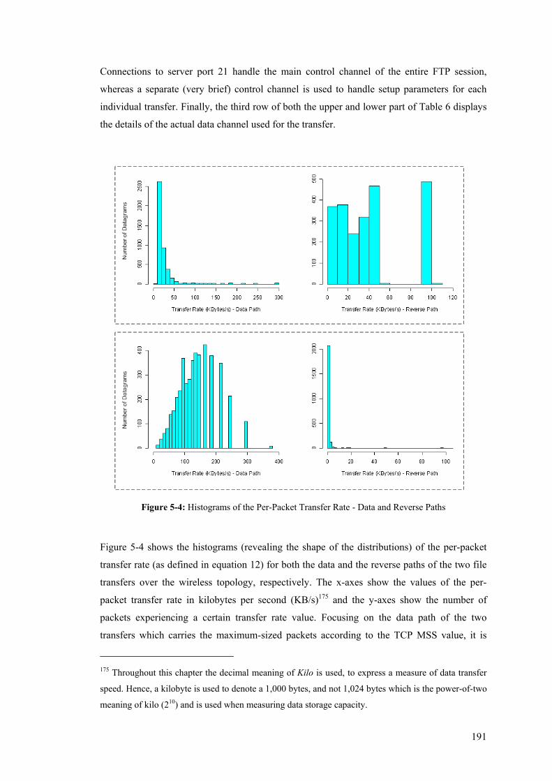
191

Connections to server port 21 handle the main control channel of the entire FTP session,

whereas a separate (very brief) control channel is used to handle setup parameters for each

individual transfer. Finally, the third row of both the upper and lower part of Table 6 displays

the details of the actual data channel used for the transfer.

Figure 5-4: Histograms of the Per-Packet Transfer Rate - Data and Reverse Paths

Figure 5-4 shows the histograms (revealing the shape of the distributions) of the per-packet

transfer rate (as defined in equation 12) for both the data and the reverse paths of the two file

transfers over the wireless topology, respectively. The x-axes show the values of the per-

packet transfer rate in kilobytes per second (KB/s)175 and the y-axes show the number of

packets experiencing a certain transfer rate value. Focusing on the data path of the two

transfers which carries the maximum-sized packets according to the TCP MSS value, it is

175 Throughout this chapter the decimal meaning of Kilo is used, to express a measure of data transfer

speed. Hence, a kilobyte is used to denote a 1,000 bytes, and not 1,024 bytes which is the power-of-two

meaning of kilo (210) and is used when measuring data storage capacity.

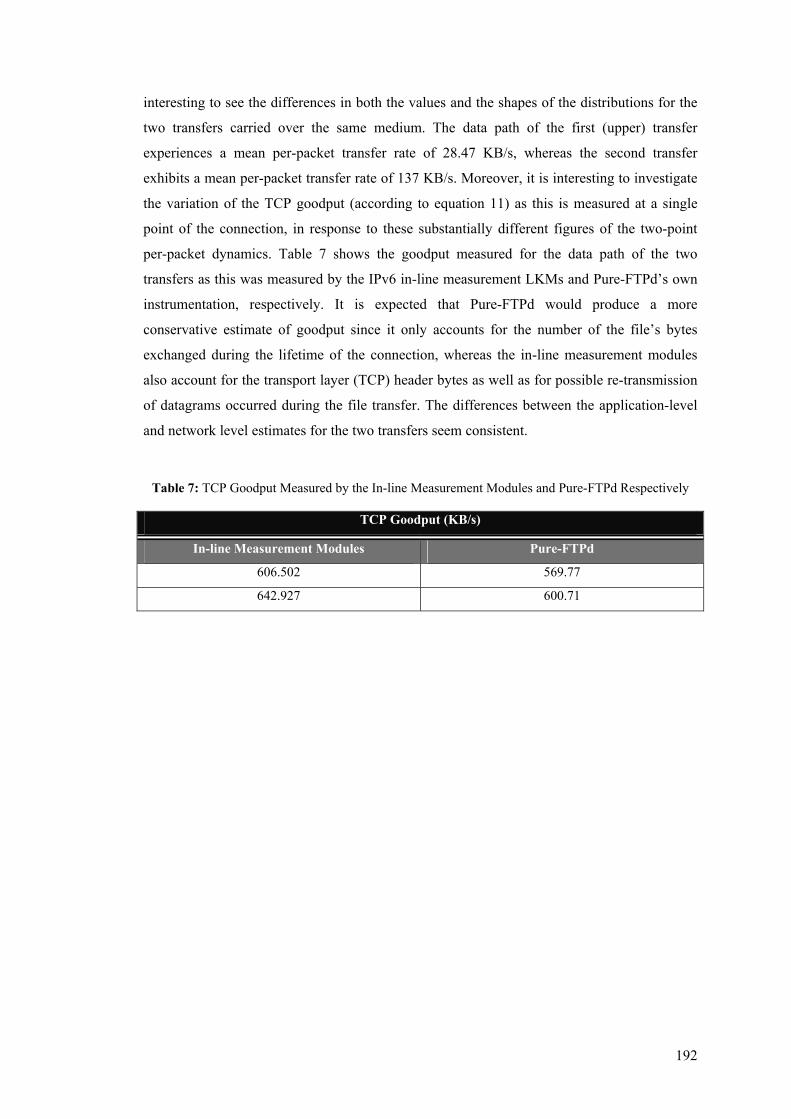
192

interesting to see the differences in both the values and the shapes of the distributions for the

two transfers carried over the same medium. The data path of the first (upper) transfer

experiences a mean per-packet transfer rate of 28.47 KB/s, whereas the second transfer

exhibits a mean per-packet transfer rate of 137 KB/s. Moreover, it is interesting to investigate

the variation of the TCP goodput (according to equation 11) as this is measured at a single

point of the connection, in response to these substantially different figures of the two-point

per-packet dynamics. Table 7 shows the goodput measured for the data path of the two

transfers as this was measured by the IPv6 in-line measurement LKMs and Pure-FTPd’s own

instrumentation, respectively. It is expected that Pure-FTPd would produce a more

conservative estimate of goodput since it only accounts for the number of the file’s bytes

exchanged during the lifetime of the connection, whereas the in-line measurement modules

also account for the transport layer (TCP) header bytes as well as for possible re-transmission

of datagrams occurred during the file transfer. The differences between the application-level

and network level estimates for the two transfers seem consistent.

Table 7: TCP Goodput Measured by the In-line Measurement Modules and Pure-FTPd Respectively

TCP Goodput (KB/s)

In-line Measurement Modules Pure-FTPd

606.502 569.77

642.927 600.71

193

Focusing on the estimates produced by the in-line measurement modules for the two file

transfers, the ratio between the mean per-packet transfer times ( 28.47 /137 0.208≈ ) is

largely different from the ratio of the overall goodputs ( 606.502 / 642.927 0.94≈ ), which is

much closer to 1, indicating the similarity in the two goodput measures.

In order to investigate the differences between the values of the two-point per-packet transfer

rate and the single-point aggregate per-connection goodput, one can take a closer look at how

these metrics are computed. Based on equation 12, the mean per-packet transfer rate for a

connection consisting of n packets is calculated as follows:

1

1 ni

r si i i

pRn t t=

=−∑ (20)

where ip is the size of each packet and r si it t− is the one-way delay experienced by this

packet between the sender and the receiver. Accordingly, the overall goodput of a connection

(based on equation 10) consisting of n packets is calculated as follows:

1

1

n

iir rn

pG

t t==−

∑ (21)

where ip is the size of each packet and 1r rnt t− is the total transfer time computed as the

difference between the times the last and the first packets of the connection arrived at the

receiver. For the data path of a connection it is safe to assume a common packet size ip p=

for all datagrams exchanged. Indeed, this is verified by the measurement traces which show

that, apart from very few datagrams that initiate and terminate the connection, all the rest are

maximum-sized datagrams specified by the negotiated TCP MSS value between the two

communication ends. Based on equations 20 and 21 the ratio between the mean per-packet

transfer time and the connection goodput is:

( )1 1

11 1

1

1

1

11 1 1

1( )

( )

i

n ni

r sr s r sp pi ii ii i i i

n

r ri r rni n

r rn

r s r ri i n

r si ir r

n

p ppt tn t t n t tR

np npG pt t t t

t t

t t t tn n t t

t t

== =

=

−− − = = = =

− −−

− −= =

−−

∑ ∑

∑ (22)

In the experiments over the wireless topology, this ratio has been less than one (1), since the

goodput in both cases was larger than the mean per-packet transfer rate. Hence,

194

1 11 ( )( )

r r r rr sn ni ir s

i i

t t t t t tnn t t

− −< ⇒ < −

− (23)

Equation 23 implies that for the RG

ratio to be less than one, the mean per-packet one-way

delay needs to be greater than the average per-packet arrival time, as this is computed by the

total transfer time divided by the number of packets. Table 8 summarises these metrics for the

two file transfers over the wireless topology.

Table 8: Average Arrival Time and Mean One-Way Delay for the two File Transfers

1r rnt t

n−

( )r si it t−

2.373 ms 82.48 ms

2.237 ms 13.56 ms

It is evident from Table 8 that the mean one-way delay is in both cases substantially greater

than the average packet arrival time and hence the mean per-packet transfer time much less

than the overall goodput of the connections. What is also interesting to note is that while the

average packet arrival time is similar between the two transfers (and hence the goodput is also

similar), the mean per-packet one-way delay is substantially diverse.

Figure 5-5 shows the packet inter-departure time from the sender plotted over the packet inter-

arrival time at the receiver for the pairs of successive packets of the data paths of the two file

transfers.

Figure 5-5: Packet Inter-Departure vs. Inter-Arrival Times - Data Path

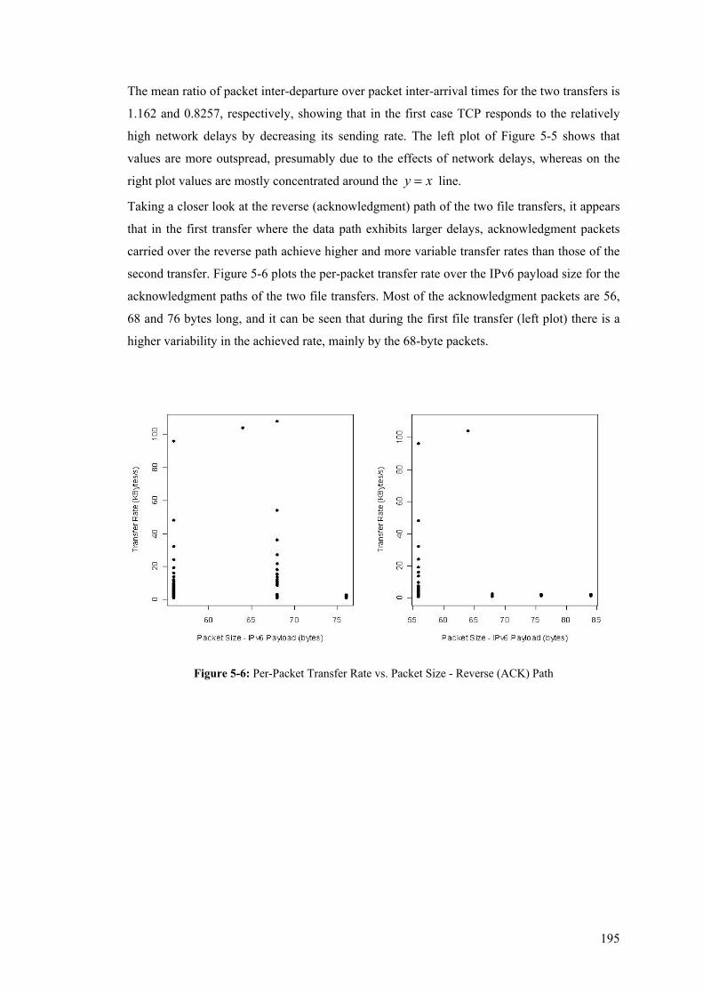
195

The mean ratio of packet inter-departure over packet inter-arrival times for the two transfers is

1.162 and 0.8257, respectively, showing that in the first case TCP responds to the relatively

high network delays by decreasing its sending rate. The left plot of Figure 5-5 shows that

values are more outspread, presumably due to the effects of network delays, whereas on the

right plot values are mostly concentrated around the y x= line.

Taking a closer look at the reverse (acknowledgment) path of the two file transfers, it appears

that in the first transfer where the data path exhibits larger delays, acknowledgment packets

carried over the reverse path achieve higher and more variable transfer rates than those of the

second transfer. Figure 5-6 plots the per-packet transfer rate over the IPv6 payload size for the

acknowledgment paths of the two file transfers. Most of the acknowledgment packets are 56,

68 and 76 bytes long, and it can be seen that during the first file transfer (left plot) there is a

higher variability in the achieved rate, mainly by the 68-byte packets.

Figure 5-6: Per-Packet Transfer Rate vs. Packet Size - Reverse (ACK) Path

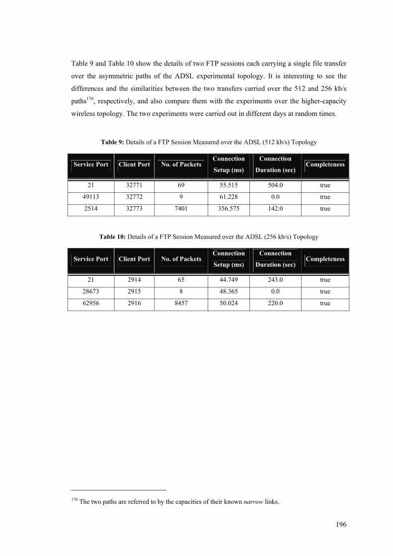
196

Table 9 and Table 10 show the details of two FTP sessions each carrying a single file transfer

over the asymmetric paths of the ADSL experimental topology. It is interesting to see the

differences and the similarities between the two transfers carried over the 512 and 256 kb/s

paths176, respectively, and also compare them with the experiments over the higher-capacity

wireless topology. The two experiments were carried out in different days at random times.

Table 9: Details of a FTP Session Measured over the ADSL (512 kb/s) Topology


Setup (ms)

Connection


21 32771 69 55.515 504.0 true

49113 32772 9 61.228 0.0 true

2514 32773 7401 356.575 142.0 true

Table 10: Details of a FTP Session Measured over the ADSL (256 kb/s) Topology


Setup (ms)

Connection


21 2914 65 44.749 243.0 true

28673 2915 8 48.365 0.0 true

62956 2916 8457 50.024 220.0 true

176 The two paths are referred to by the capacities of their known narrow links.

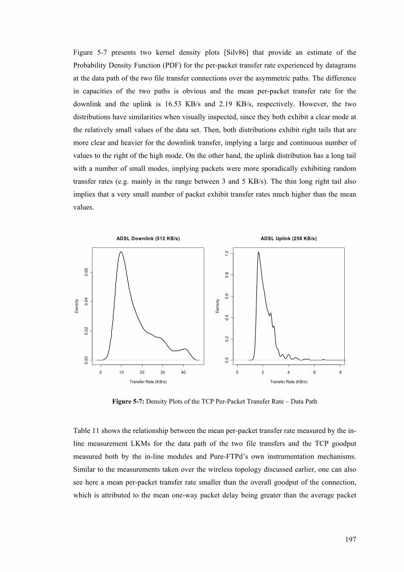
197

Figure 5-7 presents two kernel density plots [Silv86] that provide an estimate of the

Probability Density Function (PDF) for the per-packet transfer rate experienced by datagrams

at the data path of the two file transfer connections over the asymmetric paths. The difference

in capacities of the two paths is obvious and the mean per-packet transfer rate for the

downlink and the uplink is 16.53 KB/s and 2.19 KB/s, respectively. However, the two

distributions have similarities when visually inspected, since they both exhibit a clear mode at

the relatively small values of the data set. Then, both distributions exhibit right tails that are

more clear and heavier for the downlink transfer, implying a large and continuous number of

values to the right of the high mode. On the other hand, the uplink distribution has a long tail

with a number of small modes, implying packets were more sporadically exhibiting random

transfer rates (e.g. mainly in the range between 3 and 5 KB/s). The thin long right tail also

implies that a very small number of packet exhibit transfer rates much higher than the mean

values.

0 10 20 30 40

0.00

0.02

0.04

0.06

ADSL Downlink (512 KB/s)

Transfer Rate (KB/s)

Den

sity

0 2 4 6 8

0.0

0.2

0.4

0.6

0.8

1.0

ADSL Uplink (256 KB/s)

Transfer Rate (KB/s)

Den

sity

Figure 5-7: Density Plots of the TCP Per-Packet Transfer Rate – Data Path

Table 11 shows the relationship between the mean per-packet transfer rate measured by the in-

line measurement LKMs for the data path of the two file transfers and the TCP goodput

measured both by the in-line modules and Pure-FTPd’s own instrumentation mechanisms.

Similar to the measurements taken over the wireless topology discussed earlier, one can also

see here a mean per-packet transfer rate smaller than the overall goodput of the connection,

which is attributed to the mean one-way packet delay being greater than the average packet

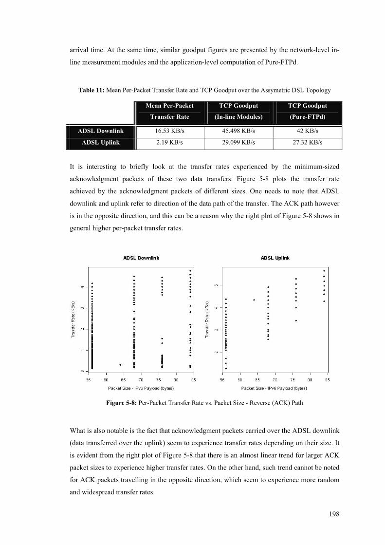
198

arrival time. At the same time, similar goodput figures are presented by the network-level in-

line measurement modules and the application-level computation of Pure-FTPd.

Table 11: Mean Per-Packet Transfer Rate and TCP Goodput over the Assymetric DSL Topology

Mean Per-Packet

Transfer Rate

TCP Goodput

(In-line Modules)

TCP Goodput

(Pure-FTPd)

ADSL Downlink 16.53 KB/s 45.498 KB/s 42 KB/s

ADSL Uplink 2.19 KB/s 29.099 KB/s 27.32 KB/s

It is interesting to briefly look at the transfer rates experienced by the minimum-sized

acknowledgment packets of these two data transfers. Figure 5-8 plots the transfer rate

achieved by the acknowledgment packets of different sizes. One needs to note that ADSL

downlink and uplink refer to direction of the data path of the transfer. The ACK path however

is in the opposite direction, and this can be a reason why the right plot of Figure 5-8 shows in

general higher per-packet transfer rates.

Figure 5-8: Per-Packet Transfer Rate vs. Packet Size - Reverse (ACK) Path

What is also notable is the fact that acknowledgment packets carried over the ADSL downlink

(data transferred over the uplink) seem to experience transfer rates depending on their size. It

is evident from the right plot of Figure 5-8 that there is an almost linear trend for larger ACK

packet sizes to experience higher transfer rates. On the other hand, such trend cannot be noted

for ACK packets travelling in the opposite direction, which seem to experience more random

and widespread transfer rates.

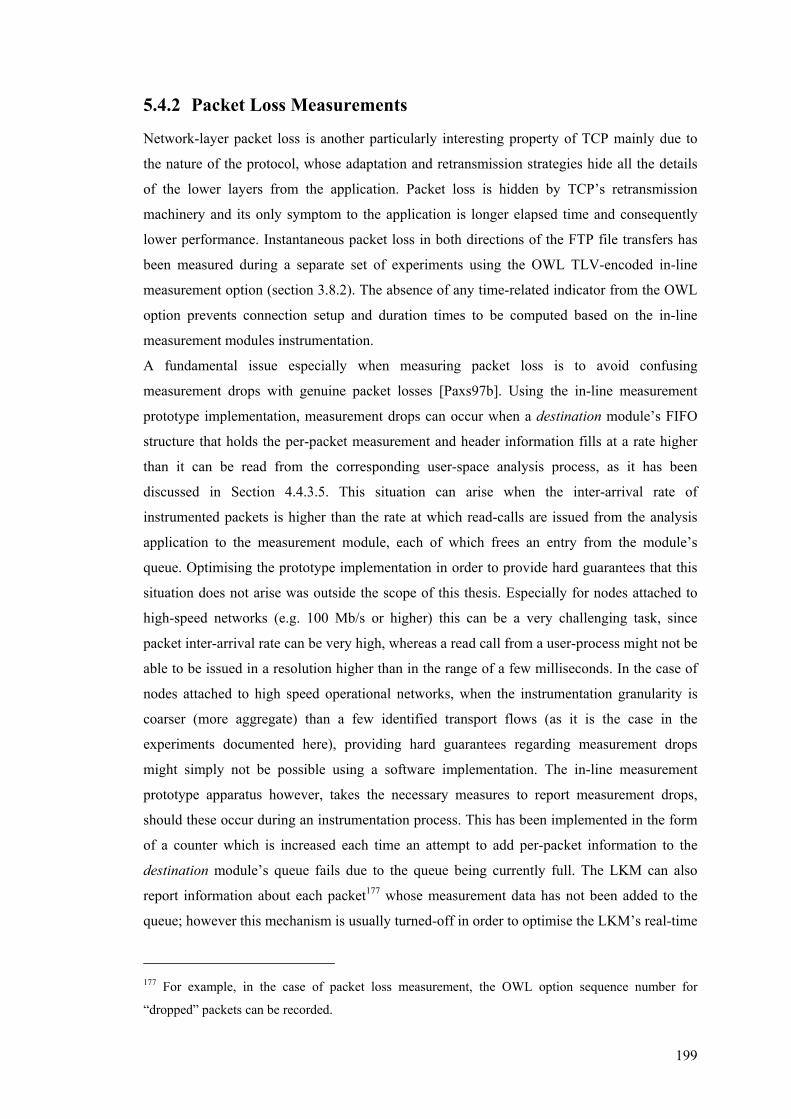
199

5.4.2 Packet Loss Measurements

Network-layer packet loss is another particularly interesting property of TCP mainly due to

the nature of the protocol, whose adaptation and retransmission strategies hide all the details

of the lower layers from the application. Packet loss is hidden by TCP’s retransmission

machinery and its only symptom to the application is longer elapsed time and consequently

lower performance. Instantaneous packet loss in both directions of the FTP file transfers has

been measured during a separate set of experiments using the OWL TLV-encoded in-line

measurement option (section 3.8.2). The absence of any time-related indicator from the OWL

option prevents connection setup and duration times to be computed based on the in-line

measurement modules instrumentation.

A fundamental issue especially when measuring packet loss is to avoid confusing

measurement drops with genuine packet losses [Paxs97b]. Using the in-line measurement

prototype implementation, measurement drops can occur when a destination module’s FIFO

structure that holds the per-packet measurement and header information fills at a rate higher

than it can be read from the corresponding user-space analysis process, as it has been

discussed in Section 4.4.3.5. This situation can arise when the inter-arrival rate of

instrumented packets is higher than the rate at which read-calls are issued from the analysis

application to the measurement module, each of which frees an entry from the module’s

queue. Optimising the prototype implementation in order to provide hard guarantees that this

situation does not arise was outside the scope of this thesis. Especially for nodes attached to

high-speed networks (e.g. 100 Mb/s or higher) this can be a very challenging task, since

packet inter-arrival rate can be very high, whereas a read call from a user-process might not be

able to be issued in a resolution higher than in the range of a few milliseconds. In the case of

nodes attached to high speed operational networks, when the instrumentation granularity is

coarser (more aggregate) than a few identified transport flows (as it is the case in the

experiments documented here), providing hard guarantees regarding measurement drops

might simply not be possible using a software implementation. The in-line measurement

prototype apparatus however, takes the necessary measures to report measurement drops,

should these occur during an instrumentation process. This has been implemented in the form

of a counter which is increased each time an attempt to add per-packet information to the

destination module’s queue fails due to the queue being currently full. The LKM can also

report information about each packet177 whose measurement data has not been added to the

queue; however this mechanism is usually turned-off in order to optimise the LKM’s real-time

177 For example, in the case of packet loss measurement, the OWL option sequence number for

“dropped” packets can be recorded.

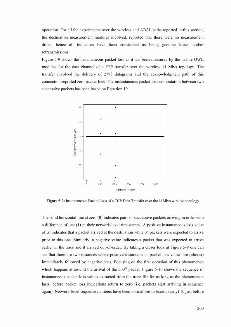
200

operation. For all the experiments over the wireless and ADSL paths reported in this section,

the destination measurement modules involved, reported that there were no measurement

drops, hence all indicators have been considered as being genuine losses and/or

retransmissions.

Figure 5-9 shows the instantaneous packet loss as it has been measured by the in-line OWL

modules for the data channel of a FTP transfer over the wireless 11 Mb/s topology. The

transfer involved the delivery of 2793 datagrams and the acknowledgment path of this

connection reported zero packet loss. The instantaneous packet loss computation between two

successive packets has been based on Equation 19.

Figure 5-9: Instantaneous Packet Loss of a TCP Data Transfer over the 11Mb/s wireless topology

The solid horizontal line at zero (0) indicates pairs of successive packets arriving in order with

a difference of one (1) in their network-level timestamps. A positive instantaneous loss value

of x indicates that a packet arrived at the destination while x packets were expected to arrive

prior to this one. Similarly, a negative value indicates a packet that was expected to arrive

earlier in the trace and it arrived out-of-order. By taking a closer look at Figure 5-9 one can

see that there are two instances where positive instantaneous packet loss values are (almost)

immediately followed by negative ones. Focusing on the first occasion of this phenomenon

which happens at around the arrival of the 500th packet, Figure 5-10 shows the sequence of

instantaneous packet loss values extracted from the trace file for as long as the phenomenon

lasts, before packet loss indications return to zero (i.e. packets start arriving in sequence

again). Network-level sequence numbers have been normalised to (exemplarily) 10 just before

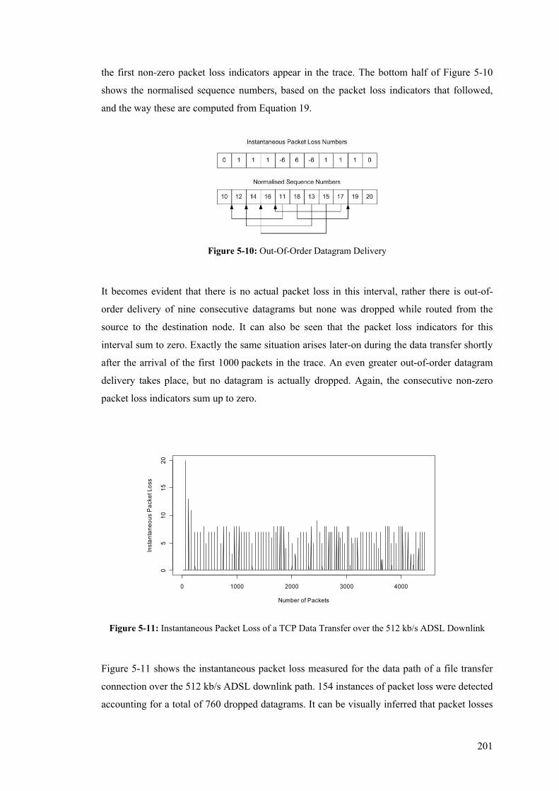
201

the first non-zero packet loss indicators appear in the trace. The bottom half of Figure 5-10

shows the normalised sequence numbers, based on the packet loss indicators that followed,

and the way these are computed from Equation 19.

Figure 5-10: Out-Of-Order Datagram Delivery

It becomes evident that there is no actual packet loss in this interval, rather there is out-of-

order delivery of nine consecutive datagrams but none was dropped while routed from the

source to the destination node. It can also be seen that the packet loss indicators for this

interval sum to zero. Exactly the same situation arises later-on during the data transfer shortly

after the arrival of the first 1000 packets in the trace. An even greater out-of-order datagram

delivery takes place, but no datagram is actually dropped. Again, the consecutive non-zero

packet loss indicators sum up to zero.

0 1000 2000 3000 4000

05

1015

20

Number of Packets

Inst

anta

neou

s P

acke

t Los

s

Figure 5-11: Instantaneous Packet Loss of a TCP Data Transfer over the 512 kb/s ADSL Downlink

Figure 5-11 shows the instantaneous packet loss measured for the data path of a file transfer

connection over the 512 kb/s ADSL downlink path. 154 instances of packet loss were detected

accounting for a total of 760 dropped datagrams. It can be visually inferred that packet losses

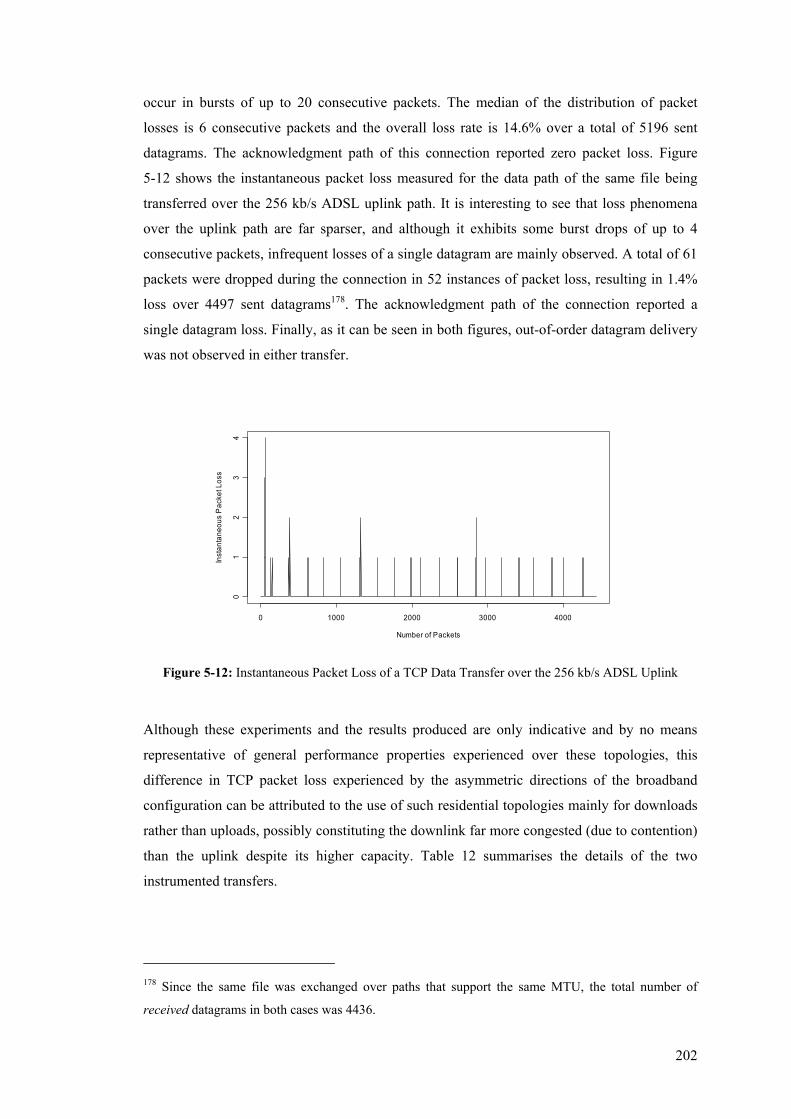
202

occur in bursts of up to 20 consecutive packets. The median of the distribution of packet

losses is 6 consecutive packets and the overall loss rate is 14.6% over a total of 5196 sent

datagrams. The acknowledgment path of this connection reported zero packet loss. Figure

5-12 shows the instantaneous packet loss measured for the data path of the same file being

transferred over the 256 kb/s ADSL uplink path. It is interesting to see that loss phenomena

over the uplink path are far sparser, and although it exhibits some burst drops of up to 4

consecutive packets, infrequent losses of a single datagram are mainly observed. A total of 61

packets were dropped during the connection in 52 instances of packet loss, resulting in 1.4%

loss over 4497 sent datagrams178. The acknowledgment path of the connection reported a

single datagram loss. Finally, as it can be seen in both figures, out-of-order datagram delivery

was not observed in either transfer.

0 1000 2000 3000 4000

01

23

4

Number of Packets

Inst

anta

neou

s P

acke

t Los

s

Figure 5-12: Instantaneous Packet Loss of a TCP Data Transfer over the 256 kb/s ADSL Uplink

Although these experiments and the results produced are only indicative and by no means

representative of general performance properties experienced over these topologies, this

difference in TCP packet loss experienced by the asymmetric directions of the broadband

configuration can be attributed to the use of such residential topologies mainly for downloads

rather than uploads, possibly constituting the downlink far more congested (due to contention)

than the uplink despite its higher capacity. Table 12 summarises the details of the two

instrumented transfers.

178 Since the same file was exchanged over paths that support the same MTU, the total number of

received datagrams in both cases was 4436.

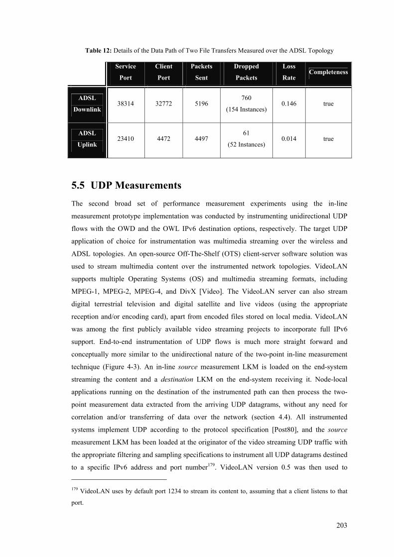
203

Table 12: Details of the Data Path of Two File Transfers Measured over the ADSL Topology

Service

Port

Client

Port

Packets

Sent

Dropped

Packets

Loss

Rate Completeness

ADSL

Downlink 38314 32772 5196

760

(154 Instances) 0.146 true

ADSL

Uplink 23410 4472 4497

61

(52 Instances) 0.014 true

5.5 UDP Measurements The second broad set of performance measurement experiments using the in-line

measurement prototype implementation was conducted by instrumenting unidirectional UDP

flows with the OWD and the OWL IPv6 destination options, respectively. The target UDP

application of choice for instrumentation was multimedia streaming over the wireless and

ADSL topologies. An open-source Off-The-Shelf (OTS) client-server software solution was

used to stream multimedia content over the instrumented network topologies. VideoLAN

supports multiple Operating Systems (OS) and multimedia streaming formats, including

MPEG-1, MPEG-2, MPEG-4, and DivX [Video]. The VideoLAN server can also stream

digital terrestrial television and digital satellite and live videos (using the appropriate

reception and/or encoding card), apart from encoded files stored on local media. VideoLAN

was among the first publicly available video streaming projects to incorporate full IPv6

support. End-to-end instrumentation of UDP flows is much more straight forward and

conceptually more similar to the unidirectional nature of the two-point in-line measurement

technique (Figure 4-3). An in-line source measurement LKM is loaded on the end-system

streaming the content and a destination LKM on the end-system receiving it. Node-local

applications running on the destination of the instrumented path can then process the two-

point measurement data extracted from the arriving UDP datagrams, without any need for

correlation and/or transferring of data over the network (section 4.4). All instrumented

systems implement UDP according to the protocol specification [Post80], and the source

measurement LKM has been loaded at the originator of the video streaming UDP traffic with

the appropriate filtering and sampling specifications to instrument all UDP datagrams destined

to a specific IPv6 address and port number179. VideoLAN version 0.5 was then used to 179 VideoLAN uses by default port 1234 to stream its content to, assuming that a client listens to that

port.

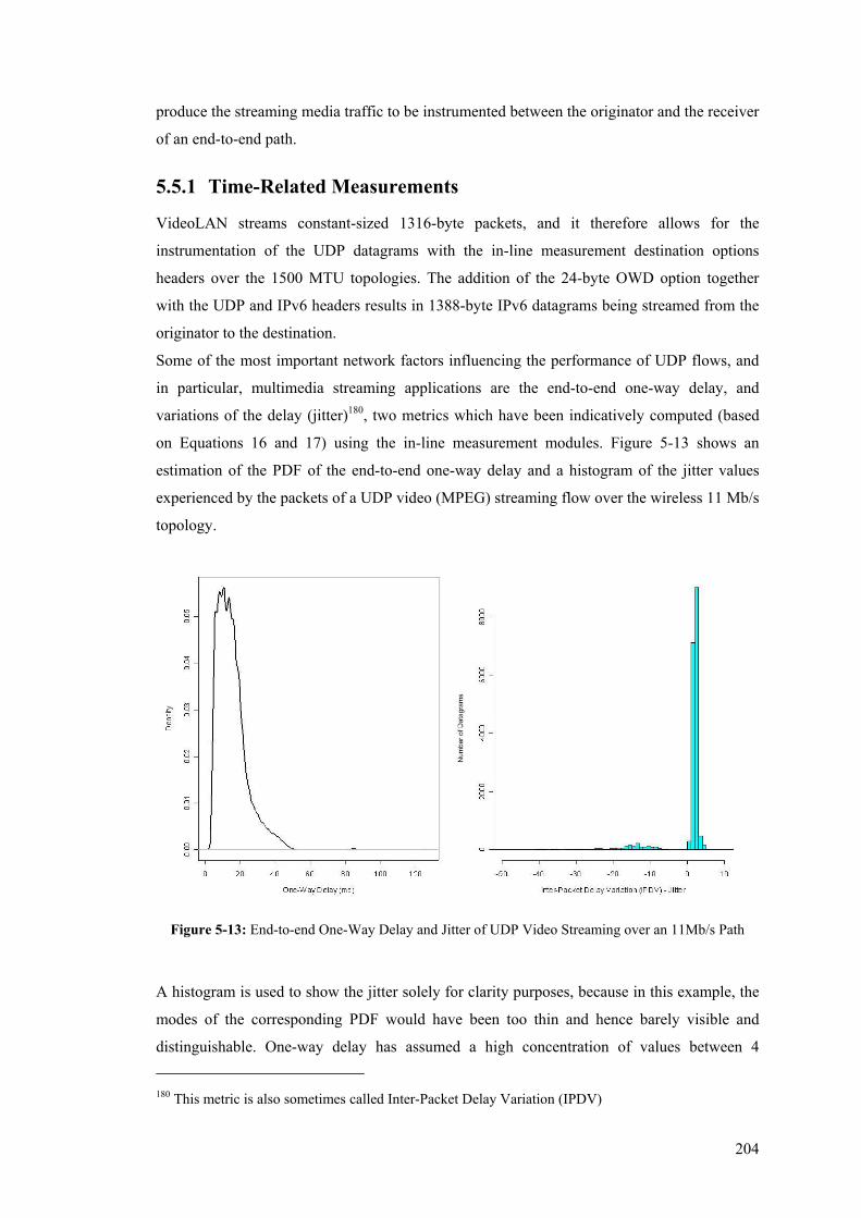
204

produce the streaming media traffic to be instrumented between the originator and the receiver

of an end-to-end path.

5.5.1 Time-Related Measurements

VideoLAN streams constant-sized 1316-byte packets, and it therefore allows for the

instrumentation of the UDP datagrams with the in-line measurement destination options

headers over the 1500 MTU topologies. The addition of the 24-byte OWD option together

with the UDP and IPv6 headers results in 1388-byte IPv6 datagrams being streamed from the

originator to the destination.

Some of the most important network factors influencing the performance of UDP flows, and

in particular, multimedia streaming applications are the end-to-end one-way delay, and

variations of the delay (jitter)180, two metrics which have been indicatively computed (based

on Equations 16 and 17) using the in-line measurement modules. Figure 5-13 shows an

estimation of the PDF of the end-to-end one-way delay and a histogram of the jitter values

experienced by the packets of a UDP video (MPEG) streaming flow over the wireless 11 Mb/s

topology.

Figure 5-13: End-to-end One-Way Delay and Jitter of UDP Video Streaming over an 11Mb/s Path

A histogram is used to show the jitter solely for clarity purposes, because in this example, the

modes of the corresponding PDF would have been too thin and hence barely visible and

distinguishable. One-way delay has assumed a high concentration of values between 4 180 This metric is also sometimes called Inter-Packet Delay Variation (IPDV)

205

(minimum) and 19 (75% quantile) milliseconds, whereas almost 25% of packets experience

delay between 19 and 50 milliseconds. Higher delays are very infrequently (and sparsely)

experienced mainly between 80 and 90 milliseconds, as it is indicated by the very small mode

of the PDF at around these values. The spikes on the high mode of the distribution that may

seem to imply some discontinuity among the popular delay values are most probably due to

the fact that one-way delay has been discretised to millisecond approximation (as it will be

discussed in Section 5.6). Jitter mainly assumes small positive values, implying a slightly

increasing trend in the one-way delay, with 89% of the observations between 0 and 5

milliseconds. At the same time some relatively large negative values can be seen mainly

between 8 and 20 milliseconds, implying (sporadic) sudden decreases in the delay of

successive packets throughout the duration of the UDP flow. Another interesting observation

can be made by looking at Figure 5-14 which shows the departure time between pairs of

successive packets from the sender and their corresponding inter-arrival time at the receiver. It

can be seen that the sender mainly transmits pairs of datagrams with steady inter-departure

time, mostly at multiples of 20 milliseconds. It is also clear that the medium has the capacity

(and available resources) to accommodate sender’s inter-packet spacing of more than or equal

to 20 milliseconds, and hence the corresponding inter-arrival times are lower. On the other

hand, it can be seen that pairs of packets departing with (close to) zero spacing exhibit large

inter-arrival times.

Figure 5-14: Packet Inter-Departure vs. Packet Inter-Arrival Times - UDP Streaming over the 11 Mb/s

Path

What is not evident from the visual inspection of Figure 5-14 is that the mean packet inter-

departure time at the sender is approximately 7 milliseconds, and that 75% of the packets are

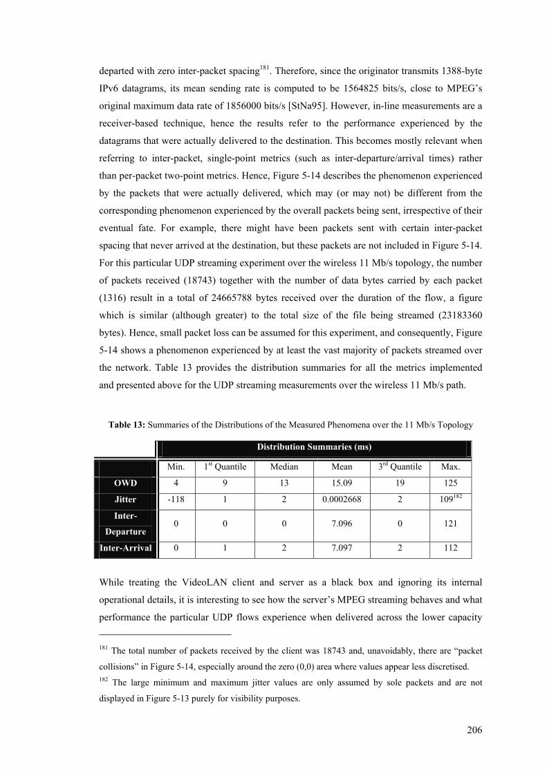
206

departed with zero inter-packet spacing181. Therefore, since the originator transmits 1388-byte

IPv6 datagrams, its mean sending rate is computed to be 1564825 bits/s, close to MPEG’s

original maximum data rate of 1856000 bits/s [StNa95]. However, in-line measurements are a

receiver-based technique, hence the results refer to the performance experienced by the

datagrams that were actually delivered to the destination. This becomes mostly relevant when

referring to inter-packet, single-point metrics (such as inter-departure/arrival times) rather

than per-packet two-point metrics. Hence, Figure 5-14 describes the phenomenon experienced

by the packets that were actually delivered, which may (or may not) be different from the

corresponding phenomenon experienced by the overall packets being sent, irrespective of their

eventual fate. For example, there might have been packets sent with certain inter-packet

spacing that never arrived at the destination, but these packets are not included in Figure 5-14.

For this particular UDP streaming experiment over the wireless 11 Mb/s topology, the number

of packets received (18743) together with the number of data bytes carried by each packet

(1316) result in a total of 24665788 bytes received over the duration of the flow, a figure

which is similar (although greater) to the total size of the file being streamed (23183360

bytes). Hence, small packet loss can be assumed for this experiment, and consequently, Figure

5-14 shows a phenomenon experienced by at least the vast majority of packets streamed over

the network. Table 13 provides the distribution summaries for all the metrics implemented

and presented above for the UDP streaming measurements over the wireless 11 Mb/s path.

Table 13: Summaries of the Distributions of the Measured Phenomena over the 11 Mb/s Topology

Distribution Summaries (ms)

Min. 1st Quantile Median Mean 3rd Quantile Max.

OWD 4 9 13 15.09 19 125

Jitter -118 1 2 0.0002668 2 109182

Inter-

Departure 0 0 0 7.096 0 121

Inter-Arrival 0 1 2 7.097 2 112

While treating the VideoLAN client and server as a black box and ignoring its internal

operational details, it is interesting to see how the server’s MPEG streaming behaves and what

performance the particular UDP flows experience when delivered across the lower capacity

181 The total number of packets received by the client was 18743 and, unavoidably, there are “packet

collisions” in Figure 5-14, especially around the zero (0,0) area where values appear less discretised. 182 The large minimum and maximum jitter values are only assumed by sole packets and are not

displayed in Figure 5-13 purely for visibility purposes.

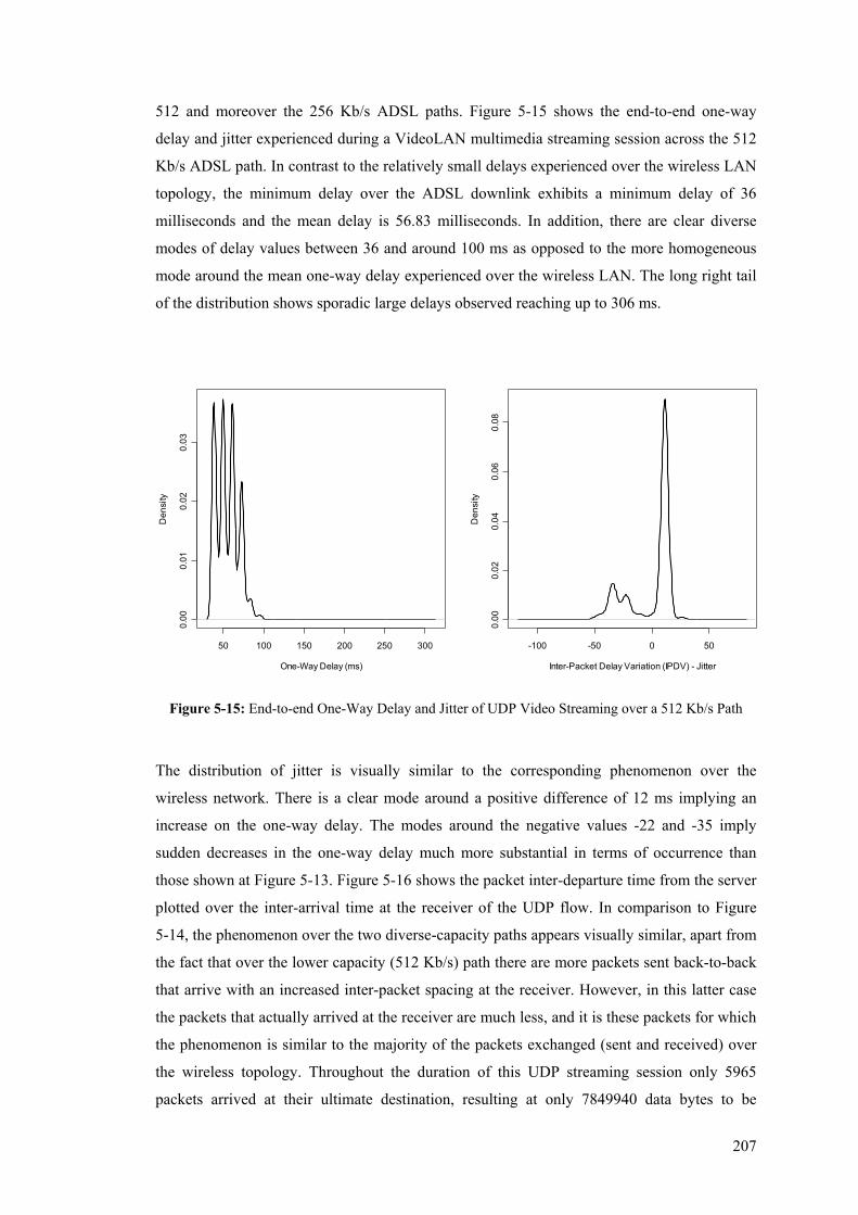
207

512 and moreover the 256 Kb/s ADSL paths. Figure 5-15 shows the end-to-end one-way

delay and jitter experienced during a VideoLAN multimedia streaming session across the 512

Kb/s ADSL path. In contrast to the relatively small delays experienced over the wireless LAN

topology, the minimum delay over the ADSL downlink exhibits a minimum delay of 36

milliseconds and the mean delay is 56.83 milliseconds. In addition, there are clear diverse

modes of delay values between 36 and around 100 ms as opposed to the more homogeneous

mode around the mean one-way delay experienced over the wireless LAN. The long right tail

of the distribution shows sporadic large delays observed reaching up to 306 ms.

50 100 150 200 250 300

0.00

0.01

0.02

0.03

One-Way Delay (ms)

Den

sity

-100 -50 0 50

0.00

0.02

0.04

0.06

0.08

Inter-Packet Delay Variation (IPDV) - Jitter

Den

sity

Figure 5-15: End-to-end One-Way Delay and Jitter of UDP Video Streaming over a 512 Kb/s Path

The distribution of jitter is visually similar to the corresponding phenomenon over the

wireless network. There is a clear mode around a positive difference of 12 ms implying an

increase on the one-way delay. The modes around the negative values -22 and -35 imply

sudden decreases in the one-way delay much more substantial in terms of occurrence than

those shown at Figure 5-13. Figure 5-16 shows the packet inter-departure time from the server

plotted over the inter-arrival time at the receiver of the UDP flow. In comparison to Figure

5-14, the phenomenon over the two diverse-capacity paths appears visually similar, apart from

the fact that over the lower capacity (512 Kb/s) path there are more packets sent back-to-back

that arrive with an increased inter-packet spacing at the receiver. However, in this latter case

the packets that actually arrived at the receiver are much less, and it is these packets for which

the phenomenon is similar to the majority of the packets exchanged (sent and received) over

the wireless topology. Throughout the duration of this UDP streaming session only 5965

packets arrived at their ultimate destination, resulting at only 7849940 data bytes to be

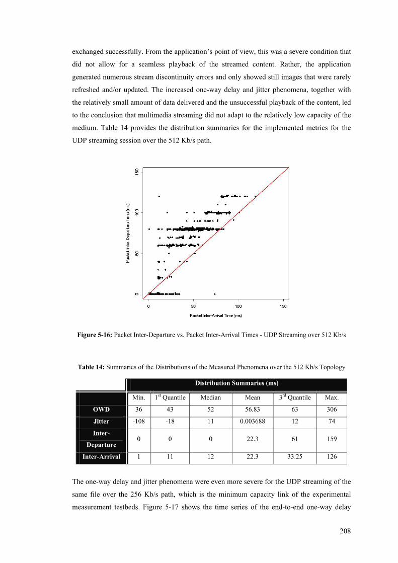
208

exchanged successfully. From the application’s point of view, this was a severe condition that

did not allow for a seamless playback of the streamed content. Rather, the application

generated numerous stream discontinuity errors and only showed still images that were rarely

refreshed and/or updated. The increased one-way delay and jitter phenomena, together with

the relatively small amount of data delivered and the unsuccessful playback of the content, led

to the conclusion that multimedia streaming did not adapt to the relatively low capacity of the

medium. Table 14 provides the distribution summaries for the implemented metrics for the

UDP streaming session over the 512 Kb/s path.

Figure 5-16: Packet Inter-Departure vs. Packet Inter-Arrival Times - UDP Streaming over 512 Kb/s

Table 14: Summaries of the Distributions of the Measured Phenomena over the 512 Kb/s Topology



OWD 36 43 52 56.83 63 306

Jitter -108 -18 11 0.003688 12 74

Inter-

Departure 0 0 0 22.3 61 159

Inter-Arrival 1 11 12 22.3 33.25 126

The one-way delay and jitter phenomena were even more severe for the UDP streaming of the

same file over the 256 Kb/s path, which is the minimum capacity link of the experimental

measurement testbeds. Figure 5-17 shows the time series of the end-to-end one-way delay

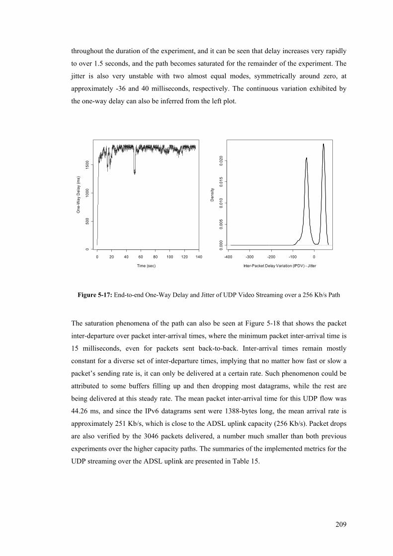
209

throughout the duration of the experiment, and it can be seen that delay increases very rapidly

to over 1.5 seconds, and the path becomes saturated for the remainder of the experiment. The

jitter is also very unstable with two almost equal modes, symmetrically around zero, at

approximately -36 and 40 milliseconds, respectively. The continuous variation exhibited by

the one-way delay can also be inferred from the left plot.

0 20 40 60 80 100 120 140

050

010

0015

00

Time (sec)

One

-Way

Del

ay (m

s)

-400 -300 -200 -100 0

0.00

00.

005

0.01

00.

015

0.02

0

Inter-Packet Delay Variation (IPDV) - Jitter

Den

sity

Figure 5-17: End-to-end One-Way Delay and Jitter of UDP Video Streaming over a 256 Kb/s Path

The saturation phenomena of the path can also be seen at Figure 5-18 that shows the packet

inter-departure over packet inter-arrival times, where the minimum packet inter-arrival time is

15 milliseconds, even for packets sent back-to-back. Inter-arrival times remain mostly

constant for a diverse set of inter-departure times, implying that no matter how fast or slow a

packet’s sending rate is, it can only be delivered at a certain rate. Such phenomenon could be

attributed to some buffers filling up and then dropping most datagrams, while the rest are

being delivered at this steady rate. The mean packet inter-arrival time for this UDP flow was

44.26 ms, and since the IPv6 datagrams sent were 1388-bytes long, the mean arrival rate is

approximately 251 Kb/s, which is close to the ADSL uplink capacity (256 Kb/s). Packet drops

are also verified by the 3046 packets delivered, a number much smaller than both previous

experiments over the higher capacity paths. The summaries of the implemented metrics for the

UDP streaming over the ADSL uplink are presented in Table 15.

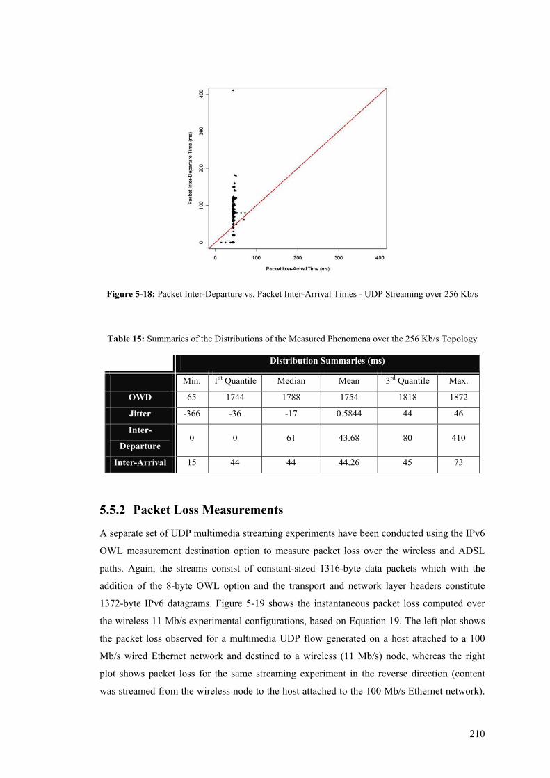
210

Figure 5-18: Packet Inter-Departure vs. Packet Inter-Arrival Times - UDP Streaming over 256 Kb/s

Table 15: Summaries of the Distributions of the Measured Phenomena over the 256 Kb/s Topology



OWD 65 1744 1788 1754 1818 1872

Jitter -366 -36 -17 0.5844 44 46

Inter-

Departure 0 0 61 43.68 80 410

Inter-Arrival 15 44 44 44.26 45 73

5.5.2 Packet Loss Measurements

A separate set of UDP multimedia streaming experiments have been conducted using the IPv6

OWL measurement destination option to measure packet loss over the wireless and ADSL

paths. Again, the streams consist of constant-sized 1316-byte data packets which with the

addition of the 8-byte OWL option and the transport and network layer headers constitute

1372-byte IPv6 datagrams. Figure 5-19 shows the instantaneous packet loss computed over

the wireless 11 Mb/s experimental configurations, based on Equation 19. The left plot shows

the packet loss observed for a multimedia UDP flow generated on a host attached to a 100

Mb/s wired Ethernet network and destined to a wireless (11 Mb/s) node, whereas the right

plot shows packet loss for the same streaming experiment in the reverse direction (content

was streamed from the wireless node to the host attached to the 100 Mb/s Ethernet network).

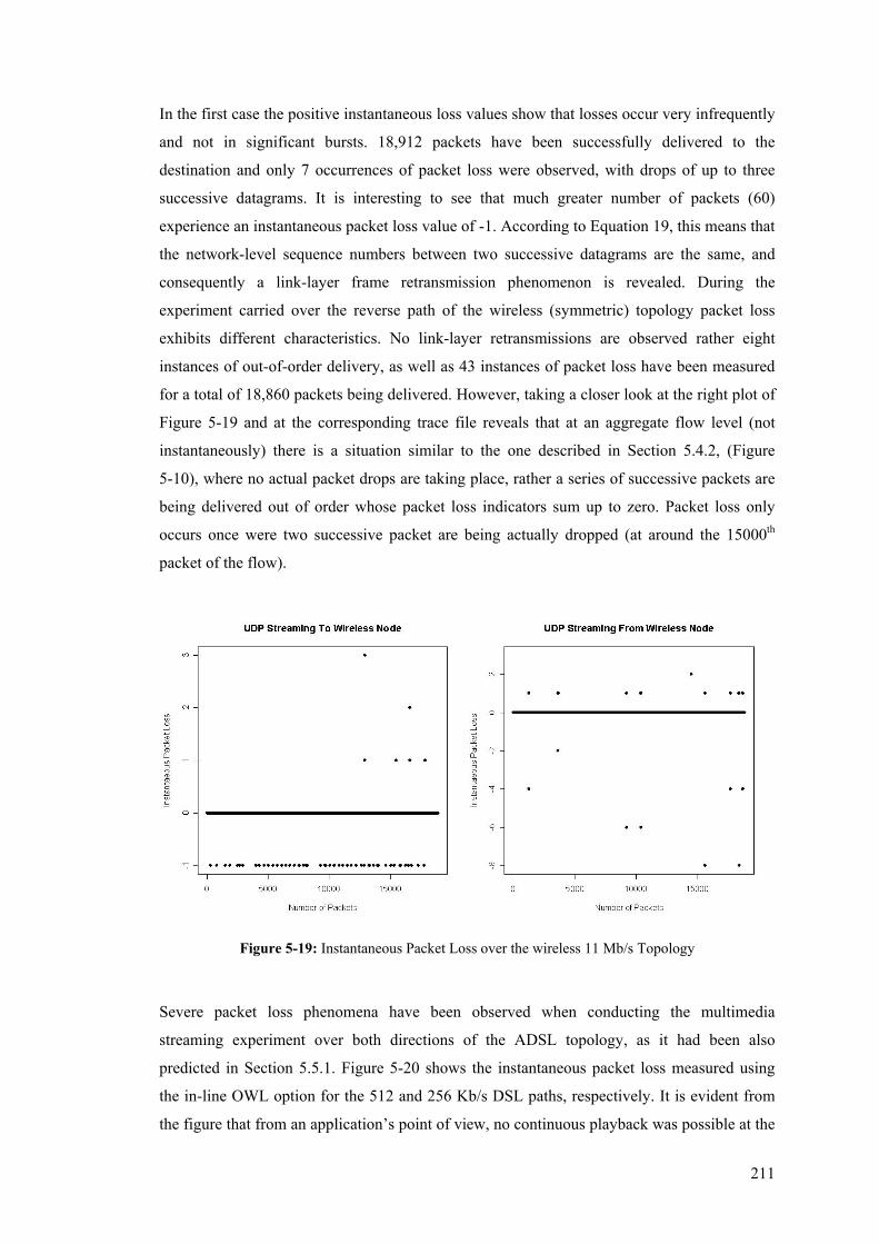
211

In the first case the positive instantaneous loss values show that losses occur very infrequently

and not in significant bursts. 18,912 packets have been successfully delivered to the

destination and only 7 occurrences of packet loss were observed, with drops of up to three

successive datagrams. It is interesting to see that much greater number of packets (60)

experience an instantaneous packet loss value of -1. According to Equation 19, this means that

the network-level sequence numbers between two successive datagrams are the same, and

consequently a link-layer frame retransmission phenomenon is revealed. During the

experiment carried over the reverse path of the wireless (symmetric) topology packet loss

exhibits different characteristics. No link-layer retransmissions are observed rather eight

instances of out-of-order delivery, as well as 43 instances of packet loss have been measured

for a total of 18,860 packets being delivered. However, taking a closer look at the right plot of

Figure 5-19 and at the corresponding trace file reveals that at an aggregate flow level (not

instantaneously) there is a situation similar to the one described in Section 5.4.2, (Figure

5-10), where no actual packet drops are taking place, rather a series of successive packets are

being delivered out of order whose packet loss indicators sum up to zero. Packet loss only

occurs once were two successive packet are being actually dropped (at around the 15000th

packet of the flow).

Figure 5-19: Instantaneous Packet Loss over the wireless 11 Mb/s Topology

Severe packet loss phenomena have been observed when conducting the multimedia

streaming experiment over both directions of the ADSL topology, as it had been also

predicted in Section 5.5.1. Figure 5-20 shows the instantaneous packet loss measured using

the in-line OWL option for the 512 and 256 Kb/s DSL paths, respectively. It is evident from

the figure that from an application’s point of view, no continuous playback was possible at the

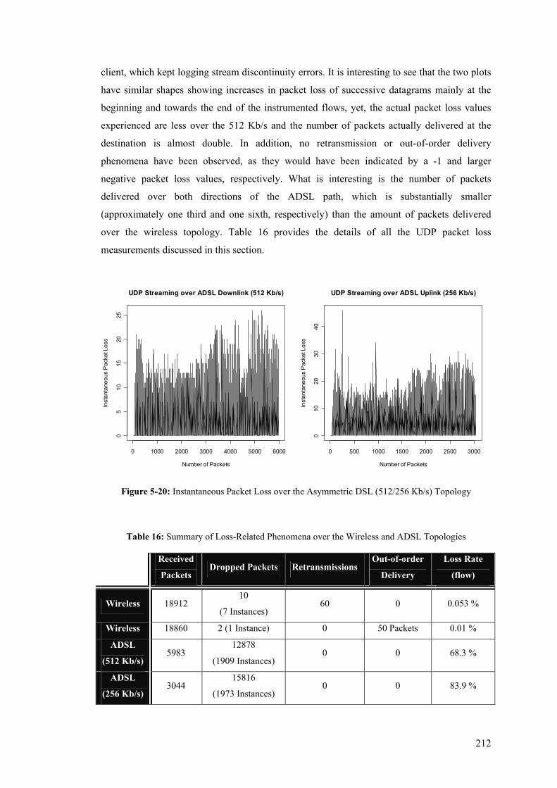
212

client, which kept logging stream discontinuity errors. It is interesting to see that the two plots

have similar shapes showing increases in packet loss of successive datagrams mainly at the

beginning and towards the end of the instrumented flows, yet, the actual packet loss values

experienced are less over the 512 Kb/s and the number of packets actually delivered at the

destination is almost double. In addition, no retransmission or out-of-order delivery

phenomena have been observed, as they would have been indicated by a -1 and larger

negative packet loss values, respectively. What is interesting is the number of packets

delivered over both directions of the ADSL path, which is substantially smaller

(approximately one third and one sixth, respectively) than the amount of packets delivered

over the wireless topology. Table 16 provides the details of all the UDP packet loss

measurements discussed in this section.

0 1000 2000 3000 4000 5000 6000

05

1015

2025

UDP Streaming over ADSL Downlink (512 Kb/s)

Number of Packets

Inst

anta

neou

s P

acke

t Los

s

0 500 1000 1500 2000 2500 3000

010

2030

40

UDP Streaming over ADSL Uplink (256 Kb/s)

Number of Packets

Inst

anta

neou

s P

acke

t Los

s

Figure 5-20: Instantaneous Packet Loss over the Asymmetric DSL (512/256 Kb/s) Topology

Table 16: Summary of Loss-Related Phenomena over the Wireless and ADSL Topologies

Received

Packets Dropped Packets Retransmissions

Out-of-order

Delivery

Loss Rate

(flow)

Wireless 18912 10

(7 Instances) 60 0 0.053 %

Wireless 18860 2 (1 Instance) 0 50 Packets 0.01 %

ADSL

(512 Kb/s) 5983

12878

(1909 Instances) 0 0 68.3 %

ADSL

(256 Kb/s) 3044

15816

(1973 Instances) 0 0 83.9 %

213

5.6 Time Synchronisation Issues Time-related per-packet metrics measured between two-points in the network such as the per-

packet transfer rate and the one-way delay, both of which have been implemented by the in-

line measurement prototype and presented in the previous sections, are relying on the clocks

of the two instrumented systems being accurately synchronised. That is, the instrumented

systems involved in a particular time-related measurement experiment need to maintain the

same notion of time with respect to a universal “correct” time, and most importantly between

them183. For the purposes of the in-line measurement which was implemented on top of

inexpensive commodity PC configurations, the Network Time Protocol (NTP) [Mill91] has

been used to achieve clock synchronisation between instrumented systems, as it was stated in

section 5.2.1. NTP is not based on the principles of directly synchronising machines with each

other, rather it is based on having all machines getting as close as possible to the correct time,

by keeping offset errors from a reference clock as low as possible. Accuracy, of course, even

for the purposes of network measurement cannot be an abstract, absolute definition rather it

relates to the properties of the measured phenomenon. Therefore, for example, an offset error

of one millisecond is acceptable for one-way delays in the range of hundreds of milliseconds

[PaVe02]. NTP is a hierarchical system of time servers whose accuracy is defined by a

number called the stratum. On top of the hierarchy, primary (stratum 1) servers are directly

synchronised to a primary reference source (stratum 0), which usually is a timecode receiver

or a calibrated atomic clock (such as, for example, a Global Positioning System (GPS)

receiver, or a Pulse Per Second (PPS) radio receiver). Lower stratum servers are then

synchronised with higher stratum servers through the Internet itself184. Both the absolute and

relative accuracy of a (NTP-synchronised) clock mainly depend on two attributes, the

difference between the time reported by the clock and the true reference time (offset), and the

rate of the clock and its difference (skew) with respect to the reference rate [MoST99]. Of the

two, the offset has traditionally generated more concern and NTP is a widely used mechanism

to enforce synchronisation. As it has been also stated in section 5.2.1, NTP provides

synchronisation accuracies in the range of a millisecond in LANs that lack many sources of

183 For the purposes of two-point measurement, it is more important to retain accurate synchronisation

between the two systems’ clocks throughout the measurement process than it is for these two clocks to

accurately maintain the notion of true time, based on some reference time source; however, the latter is

often used in order to achieve the former. 184 Regardless of the source of time for a server, its accuracy depends on its time signals, which can

vary between servers. Hence, if synchronising to true time is the objective, it is important to use

multiple time sources and verify their accuracy (The NTP daemon can choose an optimal time source

from a given set).

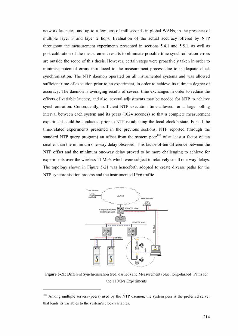
214

network latencies, and up to a few tens of milliseconds in global WANs, in the presence of

multiple layer 3 and layer 2 hops. Evaluation of the actual accuracy offered by NTP

throughout the measurement experiments presented in sections 5.4.1 and 5.5.1, as well as

post-calibration of the measurement results to eliminate possible time synchronisation errors

are outside the scope of this thesis. However, certain steps were proactively taken in order to

minimise potential errors introduced to the measurement process due to inadequate clock

synchronisation. The NTP daemon operated on all instrumented systems and was allowed

sufficient time of execution prior to an experiment, in order to achieve its ultimate degree of

accuracy. The daemon is averaging results of several time exchanges in order to reduce the

effects of variable latency, and also, several adjustments may be needed for NTP to achieve

synchronisation. Consequently, sufficient NTP execution time allowed for a large polling

interval between each system and its peers (1024 seconds) so that a complete measurement

experiment could be conducted prior to NTP re-adjusting the local clock’s state. For all the

time-related experiments presented in the previous sections, NTP reported (through the

standard NTP query program) an offset from the system peer185 of at least a factor of ten

smaller than the minimum one-way delay observed. This factor-of-ten difference between the

NTP offset and the minimum one-way delay proved to be more challenging to achieve for

experiments over the wireless 11 Mb/s which were subject to relatively small one-way delays.

The topology shown in Figure 5-21 was henceforth adopted to create diverse paths for the

NTP synchronisation process and the instrumented IPv6 traffic.

Figure 5-21: Different Synchronisation (red, dashed) and Measurement (blue, long-dashed) Paths for

the 11 Mb/s Experiments

185 Among multiple servers (peers) used by the NTP daemon, the system peer is the preferred server

that lends its variables to the system’s clock variables.

215

An additional 100 Mb/s Ethernet interface was used on the wireless node to connect directly

to the University’s backbone network and carry the NTP synchronisation messages, while the

instrumented traffic was routed through the wireless interface. The NTP offset reported over

the 100 Mb/s links was always in the range of few hundreds of microseconds. In addition, the

100 Mb/s network links to which some instrumented systems were attached, never

experienced large or highly variable delays since all experiments were carried over at least a

factor of ten narrower operational topologies which constituted the bottleneck for the

instrumented traffic. Hence, a portion of the 100 Mb/s paths used from NTP synchronisation

being common with a portion of the instrumented path (as shown in Figure 5-21) did not

cause any major side-effects to the NTP messages (such as, for example, significantly

increased network delays).

Although the OWD IPv6 measurement destination option is able to deliver timestamps with

microsecond accuracy, given the widely reported limitation of NTP not being able to

practically achieve a better than one millisecond synchronisation via an ethernet network

[PaVe02], the microsecond fraction of timestamps used for the implementation of the one-

way delay metric was not taken into consideration, and therefore, the one-way delay and jitter

results presented in the previous sections appear more discretised around integer millisecond

values.

5.7 Overhead The different classes of Internet measurement techniques, as well as broader advances in

network Measurement, Monitoring and Control (MMC) have been thoroughly discussed in

chapter 2 and a discussion of the fundamental limitations of the two broad measurement

categories (including their associated overhead), namely the active and passive measurements,

has been provided at the beginning of chapter 3. Providing insight into the operation of the

network is a task conceptually coupled with the control plane of the Internet, since it does not

directly facilitate and/or improve forwarding of the operational traffic, rather it attempts to

reveal how this traffic is treated by the infrastructure and/or how the infrastructure operates at

certain time intervals or under different traffic loads. This conceptual separation between the

data and the control planes makes activities that concentrate on the latter to be subject to

rigorous critiques regarding their associated overhead186. The overhead associated with the

IPv6-based in-line measurement technique can be classified to overhead incurred by the

technique itself and overhead incurred by a particular instantiation of a measurement system

or prototype that implements in-line measurements. Of course, the overhead of a particular 186 For example, a 20-octet measurement protocol header may be more readily considered as network

overhead than the 20-octet TCP header which is necessary to carry operational data end-to-end.

216

measurement technique needs to be jointly considered with their ability to measure or

approximate network phenomena experienced by the operational traffic. Hence, for example,

ICMP-based active measurement incur additional network load at certain time intervals and

they measure specific metrics related to the performance experienced by the probe traffic,

which may or may not approximate the performance experienced by the operational traffic.

Particular instantiations of ICMP-based measurement such as, for example, the ping utility on

a Linux platform incurs by default an additional load of 84-byte IP datagrams per second,

until stopped. On the other hand, packet monitoring techniques do not incur any disruption to

the network due to additional load, but blind monitoring of data has tremendous storage space

requirements before even attempting to measure specific properties of the traffic.

In-line measurements do not directly produce additional network load in the form of special-

purpose synthetic traffic which could potentially experience unique behaviour from the

Internet infrastructure. Rather, the technique uses a small fraction of a packet’s IPv6 payload

data to encapsulate the measurement indicators within the operational IPv6 traffic and then

compute a specific per-packet metric. This computation will henceforth reflect a performance

aspect experienced by the actual network traffic. Although the technique can be extensible to

directly implement a larger set of performance metrics, it also has the advantage that each

TLV-encoded measurement options header has a strictly defined size. Hence, for the two

measurement options presented and demonstrated in this thesis (the OWD and OWL) the

associated overhead is 24 and 8 octets of measurement traffic187 per-instrumented packet,

respectively. Additional metrics that could potentially be defined in terms of a separate IPv6

TLV-encoded option would also have a fixed-sized overhead per-instrumented packet, and not

an implementation-specific variable overhead, as it is the case with protocols that incorporate

variable-length options fields, like the existing transport protocols as well as measurement

protocols such as IPMP (section 2.2.5). Table 17 indicatively shows the overhead details that

relate to the cumulative measurement data used to instrument every single packet for a

representative set of the flows whose performance details were presented in the previous

sections. Byte overhead has been computed for both the OWD and the OWL IPv6

measurement options defined in this thesis for the data and reverse paths of a TCP connection

and a unidirectional UDP streaming flow. As it can be seen from Table 17, the overhead

incurred by the piggybacked measurement data is well below 2% for flows consisting of large

packets that make optimal use of Internet resources, providing an overall efficiency for the

data exchanged over the network between 98.3 and 99.5%. Obviously, for minimum-sized

187 These also include compulsory header fields for the IPv6 destination options header and individual

options, and are not pure measurement data, which is 20 and 4 octets, respectively (sections 3.8.1 and

3.8.2).

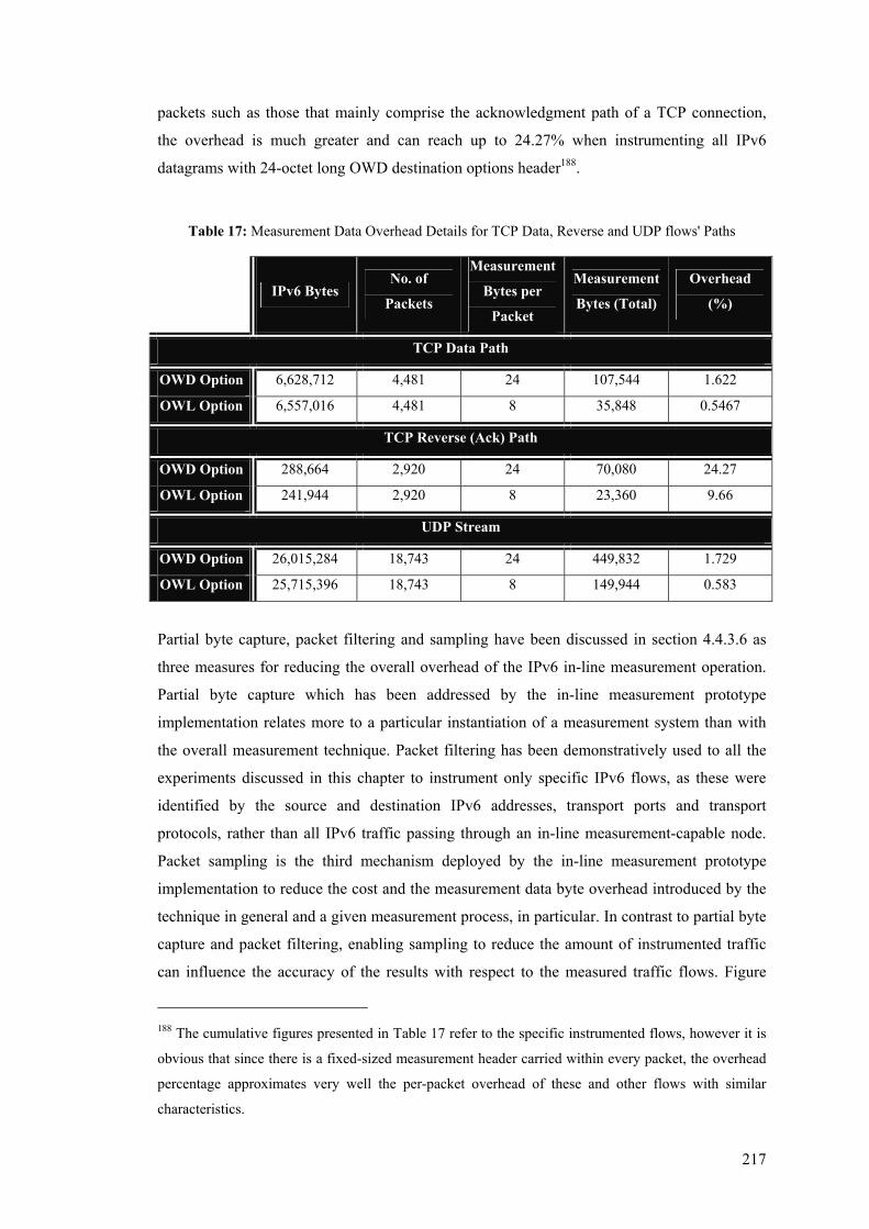
217

packets such as those that mainly comprise the acknowledgment path of a TCP connection,

the overhead is much greater and can reach up to 24.27% when instrumenting all IPv6

datagrams with 24-octet long OWD destination options header188.

Table 17: Measurement Data Overhead Details for TCP Data, Reverse and UDP flows' Paths

IPv6 Bytes No. of

Packets

Measurement

Bytes per

Packet

Measurement

Bytes (Total)

Overhead

(%)

TCP Data Path

OWD Option 6,628,712 4,481 24 107,544 1.622

OWL Option 6,557,016 4,481 8 35,848 0.5467

TCP Reverse (Ack) Path

OWD Option 288,664 2,920 24 70,080 24.27

OWL Option 241,944 2,920 8 23,360 9.66

UDP Stream

OWD Option 26,015,284 18,743 24 449,832 1.729

OWL Option 25,715,396 18,743 8 149,944 0.583

Partial byte capture, packet filtering and sampling have been discussed in section 4.4.3.6 as

three measures for reducing the overall overhead of the IPv6 in-line measurement operation.

Partial byte capture which has been addressed by the in-line measurement prototype

implementation relates more to a particular instantiation of a measurement system than with

the overall measurement technique. Packet filtering has been demonstratively used to all the

experiments discussed in this chapter to instrument only specific IPv6 flows, as these were

identified by the source and destination IPv6 addresses, transport ports and transport

protocols, rather than all IPv6 traffic passing through an in-line measurement-capable node.

Packet sampling is the third mechanism deployed by the in-line measurement prototype

implementation to reduce the cost and the measurement data byte overhead introduced by the

technique in general and a given measurement process, in particular. In contrast to partial byte

capture and packet filtering, enabling sampling to reduce the amount of instrumented traffic

can influence the accuracy of the results with respect to the measured traffic flows. Figure

188 The cumulative figures presented in Table 17 refer to the specific instrumented flows, however it is

obvious that since there is a fixed-sized measurement header carried within every packet, the overhead

percentage approximates very well the per-packet overhead of these and other flows with similar

characteristics.

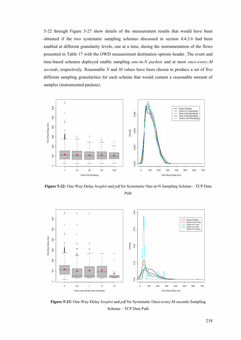
218

5-22 through Figure 5-27 show details of the measurement results that would have been

obtained if the two systematic sampling schemes discussed in section 4.4.3.6 had been

enabled at different granularity levels, one at a time, during the instrumentation of the flows

presented in Table 17 with the OWD measurement destination options header. The event and

time-based schemes deployed enable sampling one-in-N packets and at most once-every-M

seconds, respectively. Reasonable N and M values have been chosen to produce a set of five

different sampling granularities for each scheme that would contain a reasonable amount of

samples (instrumented packets).

1 10 20 50 100

010

020

030

040

050

060

0

One-in-N Sampling

One

-Way

Del

ay (m

s)

0 100 200 300 400 500 600 700

0.00

00.

002

0.00

40.

006

One-Way Delay (ms)

Den

sity

Every PacketOne-in-10 SamplingOne-in-20 SamplingOne-in-50 SamplingOne-in-100 Sampling

Figure 5-22: One-Way-Delay boxplot and pdf for Systematic One-in-N Sampling Scheme – TCP Data

Path

0 0.5 1 5 10

010

020

030

040

050

060

0

Once-every-M Seconds Sampling

One

-Way

Del

ay (m

s)

0 100 200 300 400 500 600 700

0.00

0.01

0.02

0.03

0.04

One-Way Delay (ms)

Den

sity

Every PacketOnce-in-0.5 secOnce-in-1 secOnce-in-5 secOnce-in-10 sec

Figure 5-23: One-Way-Delay boxplot and pdf for Systematic Once-every-M seconds Sampling

Scheme – TCP Data Path

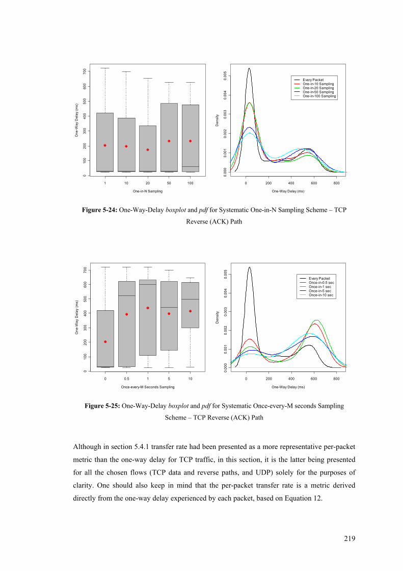
219

1 10 20 50 100

010

020

030

040

050

060

070

0

One-in-N Sampling

One

-Way

Del

ay (m

s)

0 200 400 600 800

0.00

00.

001

0.00

20.

003

0.00

40.

005

One-Way Delay (ms)

Den

sity


Figure 5-24: One-Way-Delay boxplot and pdf for Systematic One-in-N Sampling Scheme – TCP

Reverse (ACK) Path

0 0.5 1 5 10

010

020

030

040

050

060

070

0


One

-Way

Del

ay (m

s)

0 200 400 600 800

0.00

00.

001

0.00

20.

003

0.00

40.

005

One-Way Delay (ms)

Den

sity



Scheme – TCP Reverse (ACK) Path

Although in section 5.4.1 transfer rate had been presented as a more representative per-packet

metric than the one-way delay for TCP traffic, in this section, it is the latter being presented

for all the chosen flows (TCP data and reverse paths, and UDP) solely for the purposes of

clarity. One should also keep in mind that the per-packet transfer rate is a metric derived

directly from the one-way delay experienced by each packet, based on Equation 12.

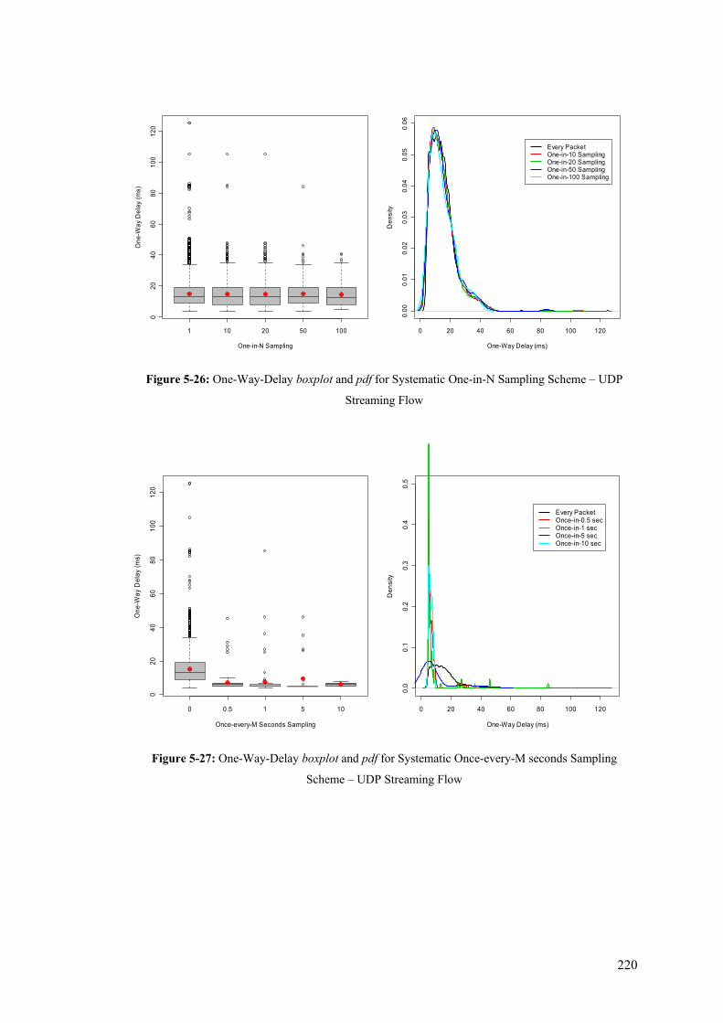
220

1 10 20 50 100

020

4060

8010

012

0

One-in-N Sampling

One

-Way

Del

ay (m

s)

0 20 40 60 80 100 120

0.00

0.01

0.02

0.03

0.04

0.05

0.06

One-Way Delay (ms)

Den

sity


Figure 5-26: One-Way-Delay boxplot and pdf for Systematic One-in-N Sampling Scheme – UDP

Streaming Flow

0 0.5 1 5 10

020

4060

8010

012

0


One

-Way

Del

ay (m

s)

0 20 40 60 80 100 120

0.0

0.1

0.2

0.3

0.4

0.5

One-Way Delay (ms)

Den

sity



Scheme – UDP Streaming Flow

221

In each of Figure 5-22 to Figure 5-27 the left plot shows the boxplots for the different

granularities of each sampling scheme deployed189. Boxplots provide a nice graphical

representation of each distribution’s summary. The lower and upper horizontal lines indicate

the minimum and maximum values, respectively, and each box represents the values between

the 1st and 3rd quantiles. The height of each box essentially provides a visual indication of the

variance of each distribution and the horizontal line within the box the median (50% quantile).

In addition, the large (red) dots reveal the mean value for each distribution, whereas points

outside the minimum-maximum boundaries represent outliers, automatically computed by the

statistical package [Rpro]. The kernel density plots [Silv86] on the right of each figure provide

an estimate of the Probability Density Function (PDF) for the measurement results obtained

by each of the sampling intervals.

An overall observation that can be made based on all figures (Figure 5-22 to Figure 5-27) is

that the event-based sampling scheme provides for a far better approximation of the one-way

delay experienced by all packets in the measured flows than the time-based scheme, for all

three different types of flows (TCP data and ACK paths, and UDP) and even for large

sampling intervals such as the one-in-100 packet sampling. Especially for the bulk TCP data

channel and the unidirectional UDP streaming flows (both of which transmit large IPv6

datagrams) the event-based sampling scheme’s approximation to the one-way delay of the

parent population is very satisfactorily accurate as demonstrated by Figure 5-22 and Figure

5-26. For the TCP reverse path that consists of small-sized acknowledgments both schemes

show fluctuations on the measured phenomenon independent from the sampling space, yet the

event-based scheme still provides a better approximation (Figure 5-24). However, this

particular TCP acknowledgment path experiences highly-variable one-way delays, something

that can certainly have influenced the accuracy of the two sampling schemes.

Table 18 indicatively shows the cost and overhead reduction of the one-in-100 packets

sampling scheme applied to the bulk TCP data and UDP streaming flows that produced

accurate estimates of the one-way delay experienced by all packets in the instrumented flows.

The measurement data overhead can be kept to a minimum of around 0.02% providing for

data efficiency in the range of 99.9%, while managing to accurately reveal the one-way delay

experienced by the instrumented flows. These measures, of course, refer to the particular

experiments and can only be used as indicative. However, they still demonstrate example test-

cases where accurate approximations of the measured phenomena can be achieved while

maintaining high data efficiency. In order to safely make generalised assumptions of flow-

189 The leftmost boxplot in each figure shows the details of the parent distribution obtained by

instrumenting every packet in the flow (i.e. every 1 packet for the event-based scheme and every 0

seconds for the time-based scheme, respectively)

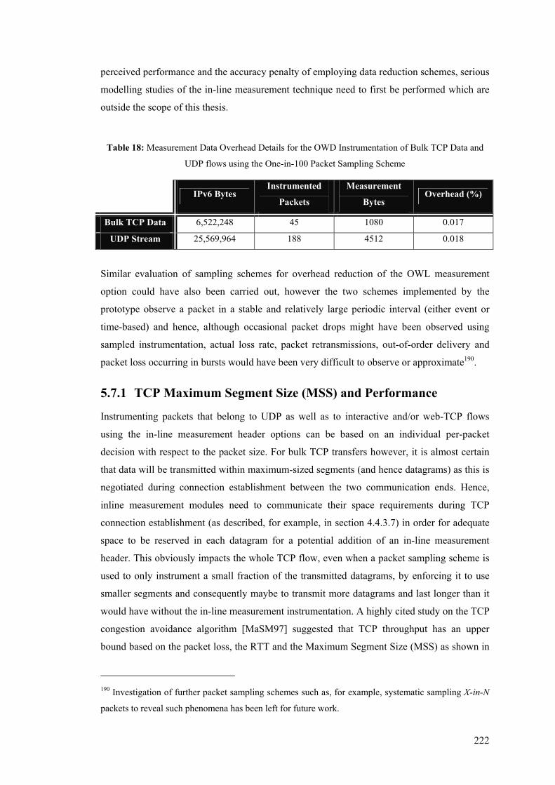
222

perceived performance and the accuracy penalty of employing data reduction schemes, serious

modelling studies of the in-line measurement technique need to first be performed which are

outside the scope of this thesis.

Table 18: Measurement Data Overhead Details for the OWD Instrumentation of Bulk TCP Data and

UDP flows using the One-in-100 Packet Sampling Scheme

IPv6 Bytes Instrumented

Packets

Measurement

Bytes Overhead (%)

Bulk TCP Data 6,522,248 45 1080 0.017

UDP Stream 25,569,964 188 4512 0.018

Similar evaluation of sampling schemes for overhead reduction of the OWL measurement

option could have also been carried out, however the two schemes implemented by the

prototype observe a packet in a stable and relatively large periodic interval (either event or

time-based) and hence, although occasional packet drops might have been observed using

sampled instrumentation, actual loss rate, packet retransmissions, out-of-order delivery and

packet loss occurring in bursts would have been very difficult to observe or approximate190.

5.7.1 TCP Maximum Segment Size (MSS) and Performance

Instrumenting packets that belong to UDP as well as to interactive and/or web-TCP flows

using the in-line measurement header options can be based on an individual per-packet

decision with respect to the packet size. For bulk TCP transfers however, it is almost certain

that data will be transmitted within maximum-sized segments (and hence datagrams) as this is

negotiated during connection establishment between the two communication ends. Hence,

inline measurement modules need to communicate their space requirements during TCP

connection establishment (as described, for example, in section 4.4.3.7) in order for adequate

space to be reserved in each datagram for a potential addition of an in-line measurement

header. This obviously impacts the whole TCP flow, even when a packet sampling scheme is

used to only instrument a small fraction of the transmitted datagrams, by enforcing it to use

smaller segments and consequently maybe to transmit more datagrams and last longer than it

would have without the in-line measurement instrumentation. A highly cited study on the TCP

congestion avoidance algorithm [MaSM97] suggested that TCP throughput has an upper

bound based on the packet loss, the RTT and the Maximum Segment Size (MSS) as shown in

190 Investigation of further packet sampling schemes such as, for example, systematic sampling X-in-N

packets to reveal such phenomena has been left for future work.

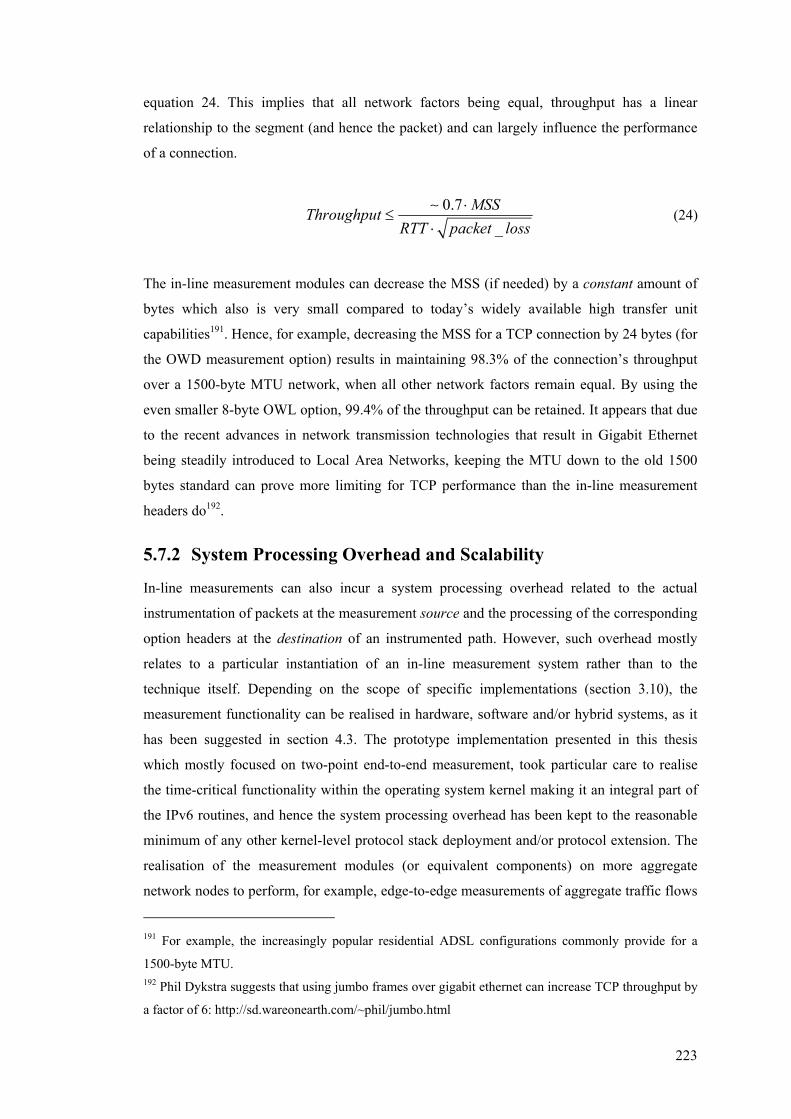
223

equation 24. This implies that all network factors being equal, throughput has a linear

relationship to the segment (and hence the packet) and can largely influence the performance

of a connection.

0.7

_MSSThroughput

RTT packet loss⋅

≤⋅∼

(24)

The in-line measurement modules can decrease the MSS (if needed) by a constant amount of

bytes which also is very small compared to today’s widely available high transfer unit

capabilities191. Hence, for example, decreasing the MSS for a TCP connection by 24 bytes (for

the OWD measurement option) results in maintaining 98.3% of the connection’s throughput

over a 1500-byte MTU network, when all other network factors remain equal. By using the

even smaller 8-byte OWL option, 99.4% of the throughput can be retained. It appears that due

to the recent advances in network transmission technologies that result in Gigabit Ethernet

being steadily introduced to Local Area Networks, keeping the MTU down to the old 1500

bytes standard can prove more limiting for TCP performance than the in-line measurement

headers do192.

5.7.2 System Processing Overhead and Scalability

In-line measurements can also incur a system processing overhead related to the actual

instrumentation of packets at the measurement source and the processing of the corresponding

option headers at the destination of an instrumented path. However, such overhead mostly

relates to a particular instantiation of an in-line measurement system rather than to the

technique itself. Depending on the scope of specific implementations (section 3.10), the

measurement functionality can be realised in hardware, software and/or hybrid systems, as it

has been suggested in section 4.3. The prototype implementation presented in this thesis

which mostly focused on two-point end-to-end measurement, took particular care to realise

the time-critical functionality within the operating system kernel making it an integral part of

the IPv6 routines, and hence the system processing overhead has been kept to the reasonable

minimum of any other kernel-level protocol stack deployment and/or protocol extension. The

realisation of the measurement modules (or equivalent components) on more aggregate

network nodes to perform, for example, edge-to-edge measurements of aggregate traffic flows

191 For example, the increasingly popular residential ADSL configurations commonly provide for a

1500-byte MTU. 192 Phil Dykstra suggests that using jumbo frames over gigabit ethernet can increase TCP throughput by

a factor of 6: http://sd.wareonearth.com/~phil/jumbo.html

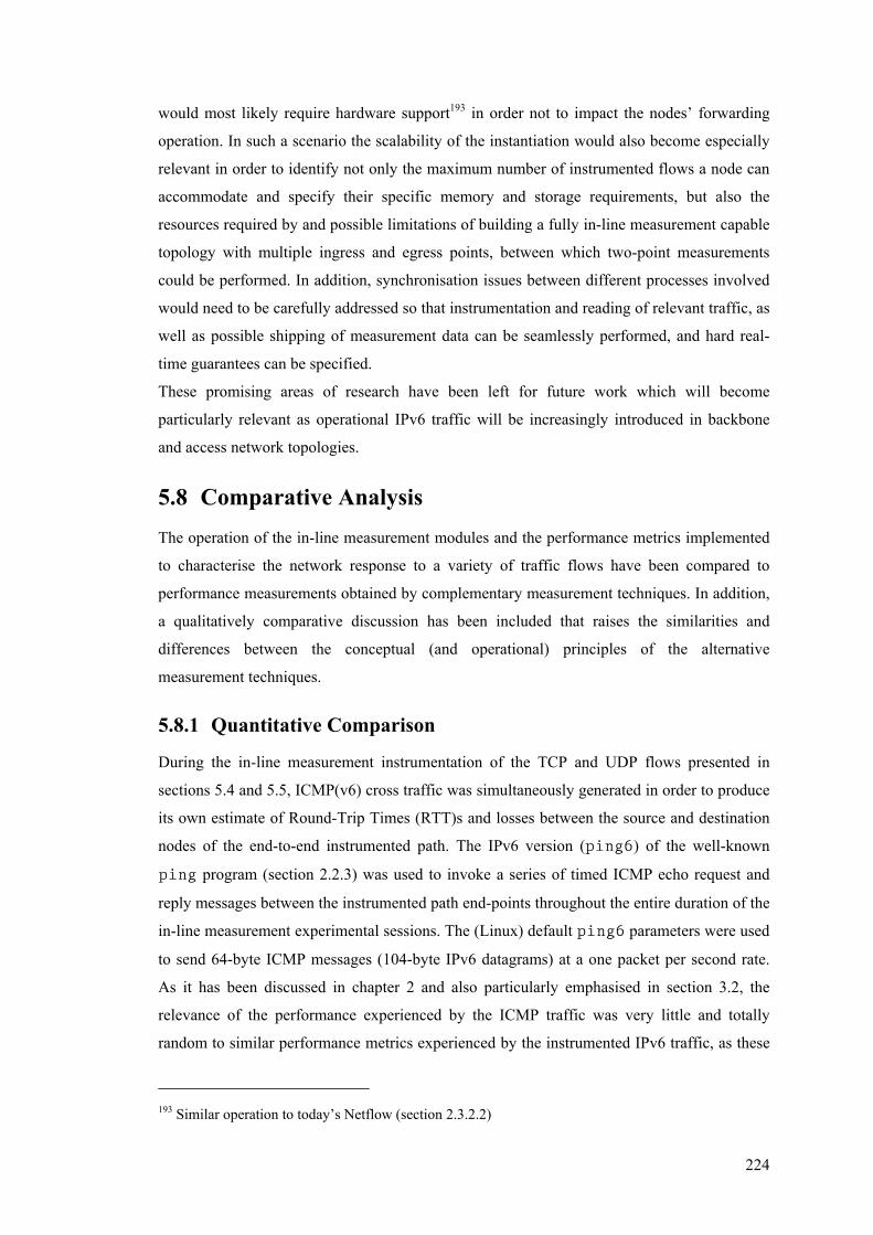
224

would most likely require hardware support193 in order not to impact the nodes’ forwarding

operation. In such a scenario the scalability of the instantiation would also become especially

relevant in order to identify not only the maximum number of instrumented flows a node can

accommodate and specify their specific memory and storage requirements, but also the

resources required by and possible limitations of building a fully in-line measurement capable

topology with multiple ingress and egress points, between which two-point measurements

could be performed. In addition, synchronisation issues between different processes involved

would need to be carefully addressed so that instrumentation and reading of relevant traffic, as

well as possible shipping of measurement data can be seamlessly performed, and hard real-

time guarantees can be specified.

These promising areas of research have been left for future work which will become

particularly relevant as operational IPv6 traffic will be increasingly introduced in backbone

and access network topologies.

5.8 Comparative Analysis The operation of the in-line measurement modules and the performance metrics implemented

to characterise the network response to a variety of traffic flows have been compared to

performance measurements obtained by complementary measurement techniques. In addition,

a qualitatively comparative discussion has been included that raises the similarities and

differences between the conceptual (and operational) principles of the alternative

measurement techniques.

5.8.1 Quantitative Comparison

During the in-line measurement instrumentation of the TCP and UDP flows presented in

sections 5.4 and 5.5, ICMP(v6) cross traffic was simultaneously generated in order to produce

its own estimate of Round-Trip Times (RTT)s and losses between the source and destination

nodes of the end-to-end instrumented path. The IPv6 version (ping6) of the well-known

ping program (section 2.2.3) was used to invoke a series of timed ICMP echo request and

reply messages between the instrumented path end-points throughout the entire duration of the

in-line measurement experimental sessions. The (Linux) default ping6 parameters were used

to send 64-byte ICMP messages (104-byte IPv6 datagrams) at a one packet per second rate.

As it has been discussed in chapter 2 and also particularly emphasised in section 3.2, the

relevance of the performance experienced by the ICMP traffic was very little and totally

random to similar performance metrics experienced by the instrumented IPv6 traffic, as these

193 Similar operation to today’s Netflow (section 2.3.2.2)

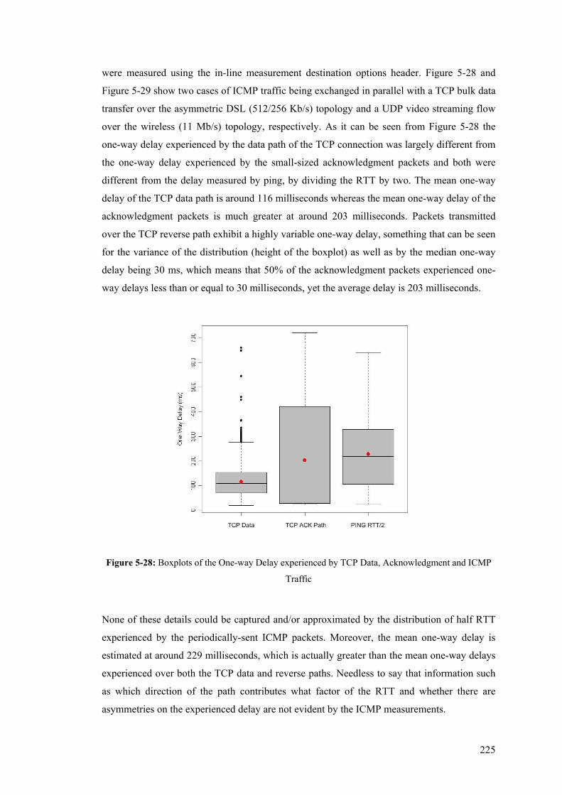
225

were measured using the in-line measurement destination options header. Figure 5-28 and

Figure 5-29 show two cases of ICMP traffic being exchanged in parallel with a TCP bulk data

transfer over the asymmetric DSL (512/256 Kb/s) topology and a UDP video streaming flow

over the wireless (11 Mb/s) topology, respectively. As it can be seen from Figure 5-28 the

one-way delay experienced by the data path of the TCP connection was largely different from

the one-way delay experienced by the small-sized acknowledgment packets and both were

different from the delay measured by ping, by dividing the RTT by two. The mean one-way

delay of the TCP data path is around 116 milliseconds whereas the mean one-way delay of the

acknowledgment packets is much greater at around 203 milliseconds. Packets transmitted

over the TCP reverse path exhibit a highly variable one-way delay, something that can be seen

for the variance of the distribution (height of the boxplot) as well as by the median one-way

delay being 30 ms, which means that 50% of the acknowledgment packets experienced one-

way delays less than or equal to 30 milliseconds, yet the average delay is 203 milliseconds.

Figure 5-28: Boxplots of the One-way Delay experienced by TCP Data, Acknowledgment and ICMP

Traffic

None of these details could be captured and/or approximated by the distribution of half RTT

experienced by the periodically-sent ICMP packets. Moreover, the mean one-way delay is

estimated at around 229 milliseconds, which is actually greater than the mean one-way delays

experienced over both the TCP data and reverse paths. Needless to say that information such

as which direction of the path contributes what factor of the RTT and whether there are

asymmetries on the experienced delay are not evident by the ICMP measurements.

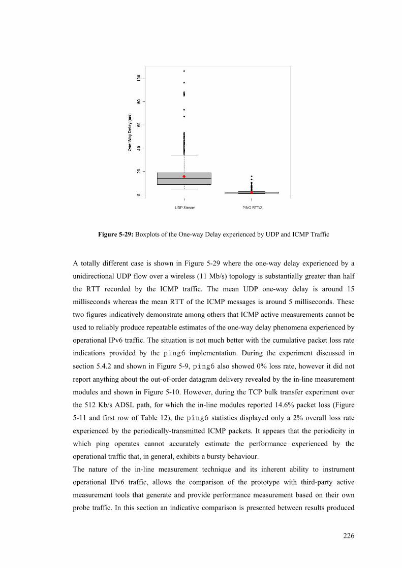
226

Figure 5-29: Boxplots of the One-way Delay experienced by UDP and ICMP Traffic

A totally different case is shown in Figure 5-29 where the one-way delay experienced by a

unidirectional UDP flow over a wireless (11 Mb/s) topology is substantially greater than half

the RTT recorded by the ICMP traffic. The mean UDP one-way delay is around 15

milliseconds whereas the mean RTT of the ICMP messages is around 5 milliseconds. These

two figures indicatively demonstrate among others that ICMP active measurements cannot be

used to reliably produce repeatable estimates of the one-way delay phenomena experienced by

operational IPv6 traffic. The situation is not much better with the cumulative packet loss rate

indications provided by the ping6 implementation. During the experiment discussed in

section 5.4.2 and shown in Figure 5-9, ping6 also showed 0% loss rate, however it did not

report anything about the out-of-order datagram delivery revealed by the in-line measurement

modules and shown in Figure 5-10. However, during the TCP bulk transfer experiment over

the 512 Kb/s ADSL path, for which the in-line modules reported 14.6% packet loss (Figure

5-11 and first row of Table 12), the ping6 statistics displayed only a 2% overall loss rate

experienced by the periodically-transmitted ICMP packets. It appears that the periodicity in

which ping operates cannot accurately estimate the performance experienced by the

operational traffic that, in general, exhibits a bursty behaviour.

The nature of the in-line measurement technique and its inherent ability to instrument

operational IPv6 traffic, allows the comparison of the prototype with third-party active

measurement tools that generate and provide performance measurement based on their own

probe traffic. In this section an indicative comparison is presented between results produced

227

by the Iperf traffic generator and the corresponding performance metrics as they were

implemented by the in-line measurement modules that were used to instrument the generated

probe traffic. Iperf is a widely used and long standing traffic generator developed by National

Laboratory for Applied Network Research (NLANR) and it was among the early active

measurement tools to incorporate IPv6 support [Iper]. Iperf version 1.7.0 which has been used

together with the in-line measurement modules to produce some comparative results, can

measure bandwidth of a TCP connection as well as the packet inter-arrival jitter and packet

loss for UDP streams of specified bandwidth. TCP goodput computed by the in-line

measurement modules has been compared and proved very similar to the FTP software’s own

instrumentation (section 5.4.1), hence the focus on this section has been on exemplary

comparing delay jitter and packet loss for unidirectional UDP streams. Iperf continuously

calculates jitter computed by the server, as described within the Real-Time Transport Protocol

(RTP) specification [ScCF96]. RTP specification defines inter-arrival jitter as being the mean

deviation of the difference in packet spacing at the receiver compared to the sender for a pair

of packets. Difference in packet spacing ( 1, )i iD − between two successively received packets

and1 i i− is computed according to Equation 18. The inter-arrival jitter is calculated

according to the following equation:

( 1, )| |16

i iD JJ J − −= + (25)

Equation 25 provides for a good noise reduction factor and an overall smoothed jitter

calculation [ScCF96]. The in-line measurement prototype software has been modified to

compute inter-arrival jitter based on Equation 25, and the OWD measurement modules have

been used with Iperf to instrument a 60-second long UDP flow of 512-byte packets sent at a

rate of 100000 bits per second over the ADSL 512 Kb/s path. Iperf was configured to provide

periodic inter-arrival jitter reports every 10 seconds. Figure 5-30 shows the smoothed inter-

arrival jitter for every 10-second interval as this has been measured by the in-line

measurement modules, and Table 19 shows the comparative results obtained for the six 10-

second intervals, as well as the overall jitter calculation for the flow, both by the in-line

measurement modules and Iperf’s own instrumentation. It can be seen that jitter experiences a

relatively higher variability during the interval between the 20th and 30th second, whereas a

sustained increase in jitter values can be observed within the last two 10-second intervals

(between the 40th and 60th seconds). Iperf has been treated as a black box and its exact internal

computations have not been investigated, and hence the jitter values displayed are assumed to

be the averages for a given sub-interval. Both the mean and median values of jitter computed

by the in-line measurement have been provided in Table 19.

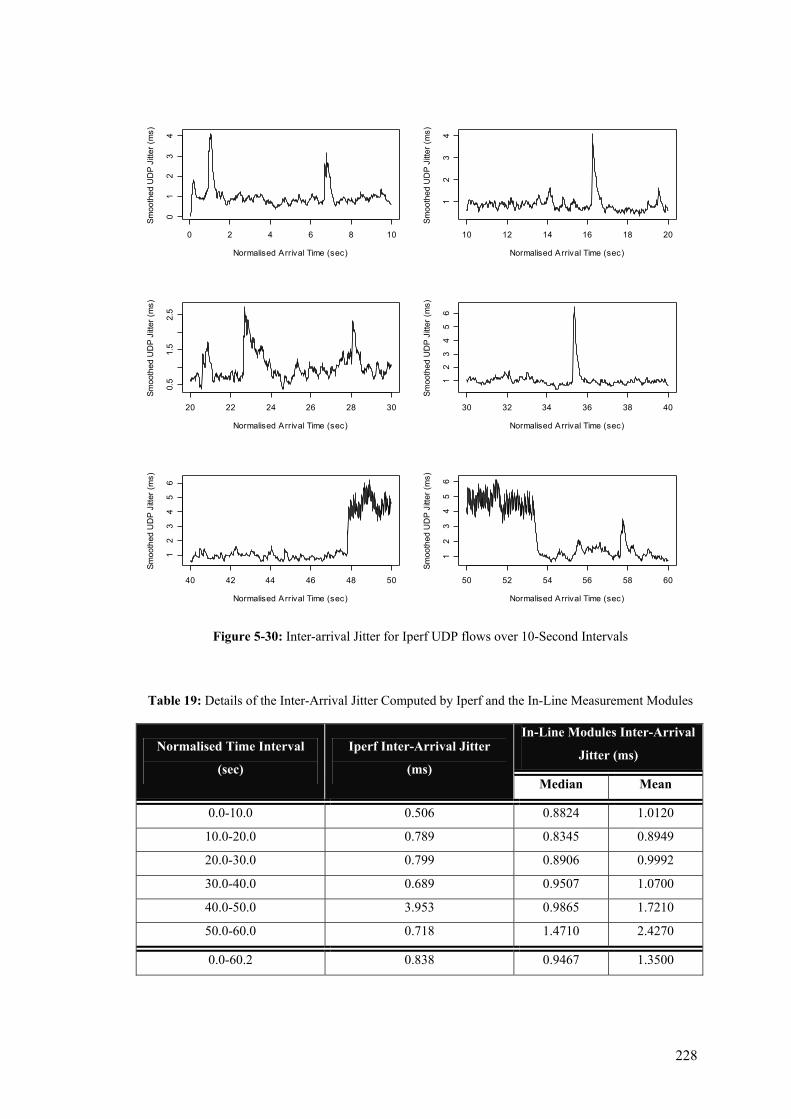
228

0 2 4 6 8 10

01

23

4

Normalised Arrival Time (sec)

Smoo

thed

UD

P Ji

tter (

ms)

10 12 14 16 18 20

12

34


Smoo

thed

UD

P Ji

tter (

ms)

20 22 24 26 28 30

0.5

1.5

2.5


Smoo

thed

UD

P Ji

tter (

ms)

30 32 34 36 38 40

12

34

56

Normalised Arrival Time (sec)Sm

ooth

ed U

DP

Jitte

r (m

s)

40 42 44 46 48 50

12

34

56


Smoo

thed

UD

P Ji

tter (

ms)

50 52 54 56 58 60

12

34

56


Smoo

thed

UD

P Ji

tter (

ms)

Figure 5-30: Inter-arrival Jitter for Iperf UDP flows over 10-Second Intervals

Table 19: Details of the Inter-Arrival Jitter Computed by Iperf and the In-Line Measurement Modules

In-Line Modules Inter-Arrival

Jitter (ms) Normalised Time Interval

(sec)

Iperf Inter-Arrival Jitter

(ms) Median Mean

0.0-10.0 0.506 0.8824 1.0120

10.0-20.0 0.789 0.8345 0.8949

20.0-30.0 0.799 0.8906 0.9992

30.0-40.0 0.689 0.9507 1.0700

40.0-50.0 3.953 0.9865 1.7210

50.0-60.0 0.718 1.4710 2.4270

0.0-60.2 0.838 0.9467 1.3500

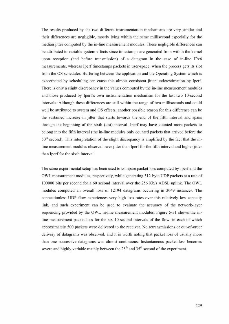
229

The results produced by the two different instrumentation mechanisms are very similar and

their differences are negligible, mostly lying within the same millisecond especially for the

median jitter computed by the in-line measurement modules. These negligible differences can

be attributed to variable system effects since timestamps are generated from within the kernel

upon reception (and before transmission) of a datagram in the case of in-line IPv6

measurements, whereas Iperf timestamps packets in user-space, when the process gets its slot

from the OS scheduler. Buffering between the application and the Operating System which is

exacerbated by scheduling can cause this almost consistent jitter underestimation by Iperf.

There is only a slight discrepancy in the values computed by the in-line measurement modules

and those produced by Iperf’s own instrumentation mechanism for the last two 10-second

intervals. Although these differences are still within the range of two milliseconds and could

well be attributed to system and OS effects, another possible reason for this difference can be

the sustained increase in jitter that starts towards the end of the fifth interval and spans

through the beginning of the sixth (last) interval. Iperf may have counted more packets to

belong into the fifth interval (the in-line modules only counted packets that arrived before the

50th second). This interpretation of the slight discrepancy is amplified by the fact that the in-

line measurement modules observe lower jitter than Iperf for the fifth interval and higher jitter

than Iperf for the sixth interval.

The same experimental setup has been used to compare packet loss computed by Iperf and the

OWL measurement modules, respectively, while generating 512-byte UDP packets at a rate of

100000 bits per second for a 60 second interval over the 256 Kb/s ADSL uplink. The OWL

modules computed an overall loss of 12194 datagrams occurring in 3049 instances. The

connectionless UDP flow experiences very high loss rates over this relatively low capacity

link, and such experiment can be used to evaluate the accuracy of the network-layer

sequencing provided by the OWL in-line measurement modules. Figure 5-31 shows the in-

line measurement packet loss for the six 10-second intervals of the flow, in each of which

approximately 500 packets were delivered to the receiver. No retransmissions or out-of-order

delivery of datagrams was observed, and it is worth noting that packet loss of usually more

than one successive datagrams was almost continuous. Instantaneous packet loss becomes

severe and highly variable mainly between the 25th and 35th second of the experiment.

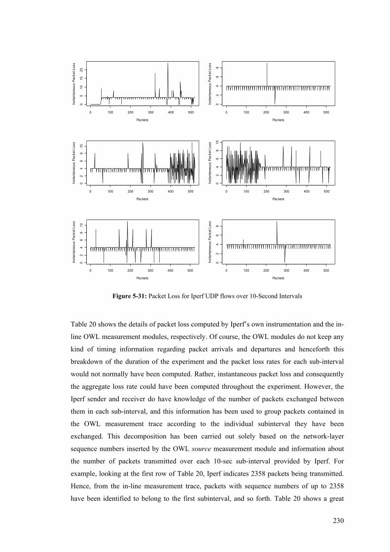
230

0 100 200 300 400 500

05

1015

20

Packets

Inst

anta

neou

s Pa

cket

Los

s

0 100 200 300 400 500

02

46

8

Packets

Inst

anta

neou

s Pa

cket

Los

s

0 100 200 300 400 500

02

46

810

Packets

Inst

anta

neou

s Pa

cket

Los

s

0 100 200 300 400 500

02

46

810

Packets

Inst

anta

neou

s Pa

cket

Los

s

0 100 200 300 400 500

02

46

810

Packets

Inst

anta

neou

s Pa

cket

Los

s

0 100 200 300 400 500

02

46

8

Packets

Inst

anta

neou

s Pa

cket

Los

s

Figure 5-31: Packet Loss for Iperf UDP flows over 10-Second Intervals

Table 20 shows the details of packet loss computed by Iperf’s own instrumentation and the in-

line OWL measurement modules, respectively. Of course, the OWL modules do not keep any

kind of timing information regarding packet arrivals and departures and henceforth this

breakdown of the duration of the experiment and the packet loss rates for each sub-interval

would not normally have been computed. Rather, instantaneous packet loss and consequently

the aggregate loss rate could have been computed throughout the experiment. However, the

Iperf sender and receiver do have knowledge of the number of packets exchanged between

them in each sub-interval, and this information has been used to group packets contained in

the OWL measurement trace according to the individual subinterval they have been

exchanged. This decomposition has been carried out solely based on the network-layer

sequence numbers inserted by the OWL source measurement module and information about

the number of packets transmitted over each 10-sec sub-interval provided by Iperf. For

example, looking at the first row of Table 20, Iperf indicates 2358 packets being transmitted.

Hence, from the in-line measurement trace, packets with sequence numbers of up to 2358

have been identified to belong to the first subinterval, and so forth. Table 20 shows a great

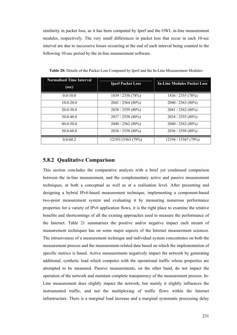
231

similarity in packet loss, as it has been computed by Iperf and the OWL in-line measurement

modules, respectively. The very small differences in packet loss that occur in each 10-sec

interval are due to successive losses occurring at the end of each interval being counted to the

following 10-sec period by the in-line measurement software.

Table 20: Details of the Packet Loss Computed by Iperf and the In-Line Measurement Modules

Normalised Time Interval

(sec) Iperf Packet Loss In-Line Modules Packet Loss

0.0-10.0 1839 / 2358 (78%) 1836 / 2355 (78%)

10.0-20.0 2041 / 2564 (80%) 2040 / 2563 (80%)

20.0-30.0 2038 / 2559 (80%) 2041 / 2562 (80%)

30.0-40.0 2037 / 2558 (80%) 2034 / 2555 (80%)

40.0-50.0 2040 / 2562 (80%) 2040 / 2562 (80%)

50.0-60.0 2036 / 2558 (80%) 2036 / 2558 (80%)

0.0-60.2 12193/15363 (79%) 12194 / 15367 (79%)

5.8.2 Qualitative Comparison

This section concludes the comparative analysis with a brief yet condensed comparison

between the in-line measurement, and the complementary active and passive measurement

techniques, at both a conceptual as well as at a realisation level. After presenting and

designing a hybrid IPv6-based measurement technique, implementing a component-based

two-point measurement system and evaluating it by measuring numerous performance

properties for a variety of IPv6 application flows, it is the right place to examine the relative

benefits and shortcomings of all the existing approaches used to measure the performance of

the Internet. Table 21 summarises the positive and/or negative impact each stream of

measurement techniques has on some major aspects of the Internet measurement sciences.

The intrusiveness of a measurement technique and individual system concentrates on both the

measurement process and the measurement-related data based on which the implementation of

specific metrics is based. Active measurements negatively impact the network by generating

additional, synthetic load which competes with the operational traffic whose properties are

attempted to be measured. Passive measurements, on the other hand, do not impact the

operation of the network and maintain complete transparency of the measurement process. In-

Line measurement does slightly impact the network, but mainly it slightly influences the

instrumented traffic, and not the multiplexing of traffic flows within the Internet

infrastructure. There is a marginal load increase and a marginal systematic processing delay

232

which can impact the performance of the measured flows marginally, as shown in the

previous sections. The measurement-related data generated on both active and inline

measurements are small in comparison with the vast amounts of data generated by passive

measurements. The reason is twofold; first, data is generated at one-point in the network while

conducting a two-point performance measurement and it might not be generated at all if the

instrumented systems also perform the analysis of the gathered data, something that is a

common approach which was also adopted by the in-line measurement prototype. And

second, it is usually only the measurement data (i.e. a fraction of the network data) that is

shipped, when needed. On the contrary, passive measurement needs to correlate data captured

in two different points in the network in order to perform two-point performance

measurements. In addition, in most cases this is a vast amount of untargeted monitoring data

that need be shipped and post-processed.

Table 21: Benefits and Shortcomings of Active, Passive, and Inline Measurement Techniques

Aspect / Property Active Measurement Passive Measurement In-Line Measurement

Impact on network

(process)

- Intrusive: Additional

Load competing for

resources

++ Non-intrusive: No

impact on network

+ Intrusive: Marginal

load increase and minor

delay might be incurred

Impact on network

(data)

+ Load generated at one

end-point

- Load generated at one

or both ends

+ Load generated at one

end point

Confidence

- Artificially-injected

traffic used to infer

performance of

operational traffic

- Test traffic may be

treated differently

- Injected traffic affects

performance

+ Measures real user

traffic

+ Measures real user

traffic

- Possibility that

instrumented traffic is

distinguishable and

treated differently

Controllability

+ Can test any traffic,

path, sampling method,

protocol, etc., at any time

- Can only measure

available traffic

- Can only measure

available traffic

- Requires an

accommodating protocol

Security / Privacy + Private, injected traffic

+ Real data not examined - Observing real traffic

-- Observation and

modification of real

traffic

Scalability Issues

+ Can be dynamically

deployed on a per-

interface basis

- Probes per interface at

ingress & egress

- Full packet capture is

+ Can be dynamically

deployed on a per node

or per interface basis

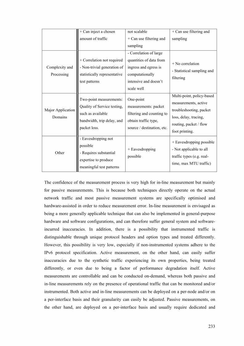
233

+ Can inject a chosen

amount of traffic

not scalable

+ Can use filtering and

sampling

+ Can use filtering and

sampling

Complexity and

Processing

+ Correlation not required

- Non-trivial generation of

statistically representative

test patterns

- Correlation of large

quantities of data from

ingress and egress is

computationally

intensive and doesn’t

scale well

+ No correlation

- Statistical sampling and

filtering

Major Application

Domains

Two-point measurements:

Quality of Service testing,

such as available

bandwidth, trip delay, and

packet loss.

One-point

measurements: packet

filtering and counting to

obtain traffic type,

source / destination, etc.

Multi-point, policy-based

measurements, active

troubleshooting, packet

loss, delay, tracing,

routing, packet / flow

foot printing.

Other

- Eavesdropping not

possible

- Requires substantial

expertise to produce

meaningful test patterns

+ Eavesdropping

possible

+ Eavesdropping possible

- Not applicable to all

traffic types (e.g. real-

time, max MTU traffic)

The confidence of the measurement process is very high for in-line measurement but mainly

for passive measurements. This is because both techniques directly operate on the actual

network traffic and most passive measurement systems are specifically optimised and

hardware-assisted in order to reduce measurement error. In-line measurement is envisaged as

being a more generally applicable technique that can also be implemented in general-purpose

hardware and software configurations, and can therefore suffer general system and software-

incurred inaccuracies. In addition, there is a possibility that instrumented traffic is

distinguishable through unique protocol headers and option types and treated differently.

However, this possibility is very low, especially if non-instrumented systems adhere to the

IPv6 protocol specification. Active measurement, on the other hand, can easily suffer

inaccuracies due to the synthetic traffic experiencing its own properties, being treated

differently, or even due to being a factor of performance degradation itself. Active

measurements are controllable and can be conducted on-demand, whereas both passive and

in-line measurements rely on the presence of operational traffic that can be monitored and/or

instrumented. Both active and in-line measurements can be deployed on a per-node and/or on

a per-interface basis and their granularity can easily be adjusted. Passive measurements, on

the other hand, are deployed on a per-interface basis and usually require dedicated and

234

expensive hardware support. The complexity of the measurement process is very large on

passive measurement systems and it usually is a multistage activity. In contrast, active and in-

line measurements can directly implement a set of performance metrics. Consequently, the

major application domain of passive measurement is traffic characterisation and network

engineering operations, whereas active and in-line measurements can be used for service-

oriented operation, such as QoS testing and end-to-end performance evaluation. Finally, in-

line measurement can potentially instrument any type of operational network data and model

the performance experienced by different traffic flows at different aggregation levels. Passive

measurement can infer properties of traffic experienced over certain topologies and existing

traffic loads, whereas active measurements need to produce statistically representative test

traffic in order to advocate the validity and relevance of the results produced.

5.9 Summary In this chapter, the in-line measurement IPv6 destination option headers have been used to

instrument a number of representative traffic flows including bulk TCP data and reverse (ack)

paths, and unidirectional UDP streaming flows, and revealed different aspects of their

perceived performance. The experiments mostly focused on measuring two-point empirical

per-packet metrics, which were also related to single-point inter-packet metrics that have

traditionally been used for Internet performance measurements, as well as to aggregate flow

metrics (such as, for example, the throughput of a bulk TCP transfer). Through experiments, it

was shown how TCP adapts its operation over different capacity Internet paths that experience

variable delays and packet drops, and how unresponsive UDP flows can saturate a low-

capacity path and cause multimedia applications to stall.

Systematic count-based sampling proved a reliable overhead reduction mechanism for TCP

data, reverse, and UDP flows, and maintained measurement accuracy even with a significantly

reduced sample space. Systematic time-based sampling did not maintain the same level of

measurement accuracy, even for relatively large sample spaces.

Through comparative analysis, it was shown that active measurement techniques based on

synthetic traffic can produce arbitrarily different results than the actual performance

experienced by the operational network traffic flows. In addition, in-line measurement

instrumentation of flows produced by a complementary measurement traffic generator (Iperf)

showed a very high level of measurement accuracy achieved by the in-line measurement

prototype implementation. A comparative discussion that focused on the major differences

between the complementary active, passive, and in-line measurement techniques, raised the

advantages of deploying in-line measurements over the operational IPv6 Internet to carefully

instrument potentially any type of traffic and assess its perceived performance.

235

Chapter 6

6Conclusions and Future

Work 6.1 Overview This thesis has described the design, prototype implementation, and evaluation through

experimentation over operational IPv6 configurations of in-line measurement, a multi-point

measurement technique able to accurately assess the actual traffic-perceived performance

between two or more Internet nodes. A thorough and critical survey of existing network

measurement techniques and particular infrastructures and tools preceded, and motivated the

definition of in-line measurement to overcome the main inherent limitations of both active and

passive measurements. The technique proposed the insertion of measurement indicators

within the actual (non-synthetic) traffic at identified points in the network, and their

subsequent observation and/or amendment elsewhere to implement several multi-point

performance metrics and reveal the network response elicited by the different operational

traffic flows, at short timescales. By exploiting IPv6 extensibility mechanisms such as the

destination options extension header definition and the selective protocol option processing,

in-line measurement has been seamlessly realised to provide an un-intrusive universal

instrumentation mechanism of the next generation Internet.

This chapter provides a summary of the work documented in this thesis and highlights its

main research contributions. Areas of future work are identified both at an infrastructural

implementation as well as at a broader research level. Concluding remarks complete this

chapter and this thesis.

236

6.2 Thesis Summary This thesis has argued that the Internet currently lacks a generic mechanism to reliably

measure and assess the different aspects of the operational traffic’s perceived performance at

short timescales. Active measurement techniques are able to measure certain performance

properties experienced by specific synthetic traffic, and passive measurements post-process

untargeted monitoring data mainly to assess aggregate traffic behaviour at relatively long

timescales, over statically configured topologies. However, the Internet is becoming an

increasingly diverse global communications environment where numerous types of traffic

aggregates are multiplexed and carried over a variety of topologies with different

infrastructural and operational characteristics. Therefore, the need for ubiquitous mechanisms

able to accurately and reliably assess the performance experienced by this largely diverse set

of traffic flows is ever increasing. This thesis presented a novel measurement technique that

can potentially become an integral part of the Internet’s next generation core forwarding

mechanism (IPv6) by seeking minimal cooperation only at identified network nodes, while

being equally applicable to any type of traffic carried on top of IPv6 over any physical

network infrastructure.

Chapter 1 raised the importance of employing measurement mechanisms to provide for

always-on quantitative assessment of Internet’s traffic-perceived performance, and their

particular relevance to the gradual evolution of the Internet into a global telecommunications

medium, where the provision of services other than best-effort will eventually become

essential. After stating the broad aims of this thesis for enabling measurement instrumentation

that can be carefully and selectively integrated with the Internet’s main forwarding operation,

the principal motivating factors were discussed, which are mainly driven by the emergence of

multi-service networks, the desire for providing differentiated levels of service over the

Internet environment, and the evolution of traffic types with varying dynamics and

multiplexing properties. The different stakeholders as well as the primary factors that

contributed to Internet measurement becoming a highly active research area were also

discussed.

Chapter 2 provided a survey of the major deployments and advances in network and Internet

measurement. The well-known classification into active and passive measurement techniques

has been adopted in this chapter, based on whether part of the measurement process is the

generation of additional network traffic, or the process simply observes the operational traffic

based on which the measurement is conducted. Yet, a further original decomposition of each

main stream of measurement techniques down to different sub-categories has been

documented, and representative developments in each category have been presented. Active

measurement infrastructures and tools have been classified based on the protocols they

237

employ and hence the type of synthetic traffic they generate to elicit the desirable response

form the network components. Passive measurement systems have been categorised based on

their operational granularity with respect to the collected measurement information (from

aggregate per-link statistics to fine-grained per-packet data).

Chapter 3 introduced the in-line measurement technique after carefully identifying the main

limitations of both active and passive measurements. The main requirements and hence

driving forces for the investigation and the definition of a novel measurement technique have

been outlined, and the feasibility of embodying such a mechanism within different layers of

current networking stacks has been discussed. The extensibility features of the next generation

Internet Protocol (IPv6) were then presented and the particular suitability of the protocol to

incorporate in-line measurement as an integral part of its operation has been raised. The

detailed definition of specific in-line measurement structures (in the form of IPv6 TLV-

encoded destination options) to directly implement unidirectional multi-point performance

metrics has been presented. The different points in the network between which multi-point in-

line measurement functionality can be deployed, as well as the consequential benefits of such

integrated measurement instrumentation mechanism have also been discussed.

Chapter 4 described the implementation of a software-based in-line measurement prototype

realised on commodity PC configurations. The decision of adopting a modular design where

specific measurements are carried out by distinct software components has been elaborated,

and the potential of the measurement modules being employed as the core components of a

distributed measurement framework has been raised. The realisation of in-line measurement

modules as Linux Dynamically Loadable Kernel Modules (LKM)s has been presented and the

cost reduction mechanisms employed by the prototype have been discussed. Higher-level

accompanying processes to consume the raw measurement indicators and implement more

synthetic performance metrics have also been briefly described.

Chapter 5 presented the evaluation of the in-line measurement prototype implementation,

through experimentation with representative Off-The-Shelf (OTS) applications’ flows, over

different capacity operational IPv6 configurations. This chapter focused on the two-point end-

to-end in-line measurement instrumentation to exemplarily implement numerous per-packet

metrics as these were perceived by flows operating over both reliable and un-reliable transport

protocols. Different aspects of the associated measurement overhead have been discussed, and

the effectiveness of the cost reduction mechanisms employed by the prototype has been

indicatively assessed. The technique was quantitatively compared to complementary

measurement tools, and a qualitatively discussion that compared the benefits and

shortcomings of active, passive and in-line measurement concluded the chapter.

238

6.3 Main Contributions The primary contributions of this thesis relate to the in-line measurement technique itself, the

way it has been specified and engineered, and its inherent characteristics which make it a

powerful instrumentation mechanism potentially capable of becoming an integral part of the

next generation Internet’s forwarding operation. Additional contributions relate to the original

taxonomy and critical survey of existing deployments in (inter-)network measurement

research, to particular benefits of the in-line measurement prototype implementation, and to

particular performance findings through the two-point end-to-end in-line measurement

instrumentation of representative traffic flows.

6.3.1 Ubiquity

In-line measurement is a network-layer instrumentation mechanism for operational IPv6

traffic. It henceforth exhibits the properties of potentially being ubiquitously applicable to all

traffic types routed over the Internet, and at the same time it constitutes a topology-neutral

mechanism, deployable between any set of nodes.

TLV-encoded in-line measurement structures can be piggybacked as IPv6 destination options

between the main network header and the higher layer (transport) header to potentially

instrument any type of IPv6 traffic and directly implement performance metrics of interest.

Hence, a single instrumentation mechanism can be used to measure the performance

experienced by the diverse set network traffic flows.

In addition, in-line measurement capability can be implemented as part of the IPv6 stack, as it

was discussed mainly in chapter 4. Therefore, the minimal measurement option processing

can potentially be integrated to the network stack operation of any IPv6-enabled device and

constitute a universally present mechanism (similar to the ICMP echo responder built in all

modern networking stacks) that can be exploited to instrument traffic from/to any IPv6 node;

the need for dedicated measurement systems usually attached to statically-provisioned

network topologies to monitor and collect aggregate traffic information is obviated. At the

same time, piggybacked measurement data can assess the network performance with respect

to its operational load without the need for additional synthetic traffic generation. This

property is particularly relevant to topologies where operators enforce usage-based charging

and the generation of additional measure traffic might be considered expensive and not

desirable.

6.3.2 Relevance to Operational Traffic Service Quality

By avoiding any reliance on synthetic traffic and through the instrumentation of the

operational IPv6 flows, in-line measurement can guarantee with a high probability that the

239

measured performance closely matches the actual network response experienced by actual

user traffic. “Heisenberg” effects in which additional synthetic traffic perturbs the network

and biases the resulting analysis can be completely avoided, and in addition, the technique has

be engineered in a way that minimises the possibility of traffic carrying measurement

indicators being treated differently than non-instrumented traffic. Indeed, using the IPv6

destination options header to encapsulate the measurement indicators, the need for defining a

distinct protocol structure is obviated and consequently identification of instrumented traffic

through a unique protocol number is prevented. At the same time, the inherent selective

processing of IPv6 destination options only by nodes whose address is identified at the

destination field of the main IPv6 header (ultimate or explicitly-specified intermediate

destinations), eliminates the concerns of instrumented datagrams being treated differently due

to en-route processing. Intermediate nodes do not process IPv6 options, and hence additional

systematic delays and/or datagram switching between the fast (hardware) and slow (software)

paths in core routers are avoided.

6.3.3 Minimal Impact on the Network

The in-line measurement instrumentation mechanism incurs a minimal impact on the network

both in terms of the additional systematic processing overhead as well as in terms of the

additional generated load. Selective measurement option processing only at well-identified

nodes in the network is guaranteed by the IPv6 specification, as opposed to IPv4 which

specified option processing en-route by all IP modules. It is envisaged that instrumented edge

systems will have the capacity to accommodate the simple measurement option processing,

whereas intermediate nodes will store-and-forward datagrams irrespective of whether they

carry measurement options or not.

Per-instrumented-packet byte overhead is also kept minimal by defining separate

measurement options to implement different performance metrics, as this has been illustrated

by the One-Way Delay (OWD) and One-Way Loss (OWL) measurement destination options

(described at sections 3.8.1 and 3.8.2). In contrast to dedicated (active) measurement protocols

like, for example, the IPMP (section 2.2.5) that try to encode multiple measurement

information within a single datagram, in-line measurement adopts an inherently modular

approach where options carry minimal information related only to a particular metric

implementation. Especially when employing further cost reduction techniques like sampling,

it was shown (section 5.7) that accurate results can be obtained while keeping the

measurement overhead as low as 0.017%, maintaining data efficiency in the order of 99%.

240

6.3.4 Direct (Targeted) Service Measurement

Through the direct implementation of per-packet performance metrics, in-line measurement is

a targeted technique to assess the service quality experienced by the operational traffic flows,

at different levels of granularity. Although post-processing of measurement data can be

employed to implement more synthetic metrics or even synthesize overall flows’ properties,

simple per-packet metrics are directly computed in real-time as part of the minimal IPv6

option processing that can be tuned through filtering to operate at micro flow or aggregate

levels. Hence, in contrast to un-targeted packet monitoring, which is the primary real-time

activity of passive measurement systems, in-line measurement directly implements some per-

packet metric that relates to a corresponding traffic-perceived service quality characteristic.

Therefore, any post-processing activity receives as input not only data relevant to a particular

measurement of a specific traffic subset, but also highly tuned measurement data as opposed

to raw (even partial) datagram traces, and can hence operate more efficiently and in short

timescales.

6.3.5 Transparency

Although in-line measurement capability can be built into networked applications by

exploiting the advanced sockets API for IPv6 to encoded and receive measurement destination

options, one of the main benefits of the technique lies in its ability to instrument application

traffic in complete transparency. This important property which is due to the enforcement of

in-line measurement at the ubiquitous IP layer has been demonstrated by the design choices of

the specific prototype implementation documented in chapter 4. Applications do not need to

be aware of any in-line measurement instrumentation taking place along the end-to-end

Internet path, and moreover, by not breaking the strict networking protocol layering, the

technique can be applied not only end-to-end but also between adequately-provisioned

Internet edge nodes (as described in section 3.9).

6.3.6 Incremental Deployment

One of the most important properties of the in-line measurement technique lies in its ability to

be incrementally deployed over the Internet, something particularly relevant due to its

operation at the traffic data path. The technique has been designed in a way that not only

ensures that the presence of measurement options in the datagrams does not incur any

additional overhead to intermediate nodes, but also that if a non-instrumented system has to

process a datagram containing in-line measurement options, its response will be graceful with

respect to the datagram’s further processing. The internal encoding of the measurement

options specifies that if a node is required (by the IPv6 specification) to process an option that

241

it does not understand, it can skip it and continue processing the datagram. By taking

particular care in order not to detrimentally affect un-supportive nodes, in-line measurement

can be deployed incrementally over the Internet, potentially enabling a gradual migration to an

environment where measurement instrumentation will be widespread, and consequently

service quality assessment of the operational traffic flows an integral part of the next

generation Internet’s operation.

6.3.7 Additional Contributions

In addition to the primary contributions of this thesis described above that relate to the

definition, design, and operation of the in-line measurement technique, the hereinabove

documented research contributed to the understanding of a specific field within the broader

Internet measurement research area, to the development of an open-system optimised

measurement prototype, as well as to the assessment of numerous performance aspects of

IPv6 traffic over complex operational configurations.

6.3.7.1 Internet Measurement Techniques Taxonomy

The description and critical review of the major developments in the Internet measurement

techniques, and their novel classification based on appropriate reasoning as presented in

chapter 2 promotes the understanding of how and why researchers have tried to instrument

parts of the Internet. At the same time, it helps the reader to identify why new contributions in

this research field are essential and how many aspects of the Internet traffic’s performance

still remain practically immeasurable.

6.3.7.2 Modular In-line Measurement System Prototype

The particular instantiation of the in-line measurement system documented in this thesis

demonstrated how minimal processing modules can be dynamically loaded (and unloaded) to

extend the functionality of a node’s networking stack and to provide for an explicitly on-off

measurement instrumentation mechanism. Chapter 4 revealed the details of an open-system

network model and IPv6 stack implementation, and critically discussed the different

implementation alternatives for the software-based in-line measurement prototype.

6.3.7.3 Per-Packet Measurement Experimental Findings

The experiments presented in chapter 5 for representative types of microflows over native and

tunnelled IPv6 configurations revealed numerous interesting properties of per-packet and flow

performance. Among others, per-packet transfer rate for bulk connection-oriented flows was

indicatively compared to aggregate flow throughput, internal packet loss phenomena such as

packet re-ordering, retransmission and successive packet drop were described, and the

242

potential of unresponsive flows easily causing saturation has been presented. In addition, the

arbitrary relevance of ICMP measurements to the operational TCP and UDP traffic-perceived

performance has been shown, and the efficacy of count-based sampling to approximate two-

point per-packet metrics due to its ability to capture the burstiness of the traffic has also been

demonstrated.

6.4 Future Directions This thesis has documented the definition and the design of in-line measurement, a novel

instrumentation technique for traffic performance evaluation over the next generation Internet

infrastructure. Several areas of future work have been identified not only to complement and

extend the implementation and evaluation aspects addressed in this thesis, but also to suggest

research directions that will couple in-line measurement instrumentation with broader network

management and traffic engineering activities. The following list summarises such future

directions that can contribute towards the integration of measurement research with network

control and operations areas.

• Distributed Measurement Architecture

Before focusing on the core measurement components of the prototype implementation and

suggesting that their operation should be decoupled from particular measurement applications,

chapter 4 briefly described a distributed measurement framework under which in-line

measurement modules can potentially be deployed. Further investigation of such measurement

architecture and precise specification of its components can benefit network operations and

management research by leading to the definition and deployment of a network-wide in-line

instrumentation system. There have already been some occasions where measurement systems

have been configured under a broader control framework providing regular services for

Internet Service Providers (ISP)s [CiMR03, GeGK01]. A distributed in-line measurement

architecture can be deployed within Autonomous System (AS) boundaries to facilitate multi-

point edge-to-edge performance measurement between network ingress and egress points.

Identification of the interdependencies between system components, the level of

(de)centralisation, and the amount of necessary correlation of measurement data to provide for

network-wide performance information from two-point measurement traces are among the

principal activities of such investigation.

243

• Large-scale End-to-end Measurements for Empirical Traffic Evaluation

Comprehensive studies of end-to-end Internet packet dynamics and routing behaviour have

been conducted by large-scale experiments involving a representative set of Internet paths

whose end-systems employed specific measurement functionality [Paxs97b]. These studies

have mainly focused on assessing the behaviour of traffic carried over the dominant TCP

transport protocol, precisely due to the lack of a global instrumentation mechanism that could

measure the performance of any type of IP traffic, at the time. Two-point end-to-end in-line

measurements can be exploited in similar ways to empirically evaluate the performance of

traffic flows over representative IPv6 Internet paths. Being a ubiquitous measurement

mechanism operating at the network layer it can facilitate the instrumentation of numerous

traffic types, and reveal their individual service quality characteristics as well as their

multiplexing properties.

• Coupling with Active Components for Traffic Engineering

It has been argued that in-line measurement can constitute an integral part of the IPv6 data

path and its main forwarding operation. In addition, the technique seeks minimal cooperation

from well-identified network nodes. This overall store-compute-and-forward model lends

itself well to programmable network technology. The possibility of deploying in-line

measurement functionality as a set of active components on a programmable network platform

[ScFS01] has already been initially investigated [PeSS04]. By continuously measuring

different performance metrics experienced by the actual traffic between two programmable

nodes, one can define additional parameters within the intra-domain protocol data structures

to reflect the network response over specific links. Such values can then be taken into

consideration when computing the link costs194 to facilitate load sensitive, service-oriented

routing. The importance of such a mechanism is better realised in the presence of virtual links

where the conventional routing metrics and link-cost assignment systems collapse.

• Processing Overhead and Scalability Assessment

Experimentation with the in-line measurement prototype system documented in this thesis has

focused on the two-point end-to-end deployment of measurement modules to assess a number

of performance properties of traffic microflows. Further experimentation can focus on the

edge-to-edge instantiation of in-line measurement between network boundaries to instrument

traffic at different levels of aggregation. The processing and system overhead of the technique

on a network edge node that handles traffic aggregates can be evaluated, and the scalability of 194 Currently, cost values are computed based on static link properties, such as the medium’s capacity.

244

particular instantiations with respect to the number of instrumented flows can be assessed.

Such investigation can become particularly important when (major) portions of the Internet

will fully migrate to IPv6, and therefore serious volumes of operational IPv6 aggregate traffic

will start appearing in the network.

• Efficacy and Applicability of further Packet Sampling Schemes

Experimental results documented in this thesis showed that systematic event-based sampling

provide a good approximation of the per-packet one-way delay experienced by the parent

population (all packets in a measured flow) for both reliable and unreliable transports, in

contrast to time-based sampling that fails to capture the burstiness of the traffic. Future work

can focus on assessing the accuracy as well as the relative cost reduction of further sampling

schemes applied at two-point performance metrics, as opposed to single-point inter-packet

metrics which have been the main focus of existing work.

• Implementation of additional Performance Metrics

This thesis focused on the definition, design, implementation and evaluation of two distinct

in-line measurement destination header options, able to implement a number of performance

metrics. Further TLV-encoded measurement options can be defined to encode additional

indicators and consequently implement further metrics to expand the features of this

measurement instrumentation mechanism.

6.5 Concluding Remarks The continuous expansion of the Internet to include a large number of heterogeneously inter-

connected systems, together with the evolution of new types of services and applications

constitute it an even more complex system with unpredictable dynamics. Appropriate

mechanisms to continuously assess the network’s traffic-perceived performance become a

necessity for such a global communications medium to be able to offer consistently

predictable performance characteristics, even in the onset of rapidly-varying traffic dynamics.

Although Internet measurement is a highly active research area, most of the recent

developments focus on the empirical analysis of distinct measurement observations over

specific network topologies, which are unique and non-reproducible, and therefore cannot

directly lead to the identification of typical or invariant factors of the network’s internal

behaviour.

This thesis has focused on the definition of a new measurement technique which, by being

able to reveal the actual service response experienced by any type of operational traffic carried

245

over the next generation Internet infrastructure, can provide a solid mechanism for always-on

traffic evaluation, and open up new horizons for measurement-based network operations.

246

References [AlCK02] Alves, M., Corsello, L., Karrenberg, D., Ögüt, C., Santcroos,. M., Sojka, R.,

Uijterwaal, H., Wilhelm, R., New Measurements with the RIPE NCC Test

Traffic Measurements Setup, Passive and Active Measurement Workshop

(PAM2002), Colorado, USA, March 25-26, 2002

[AlKZ99a] Almes, G., Kalidindi,. S., Zekauskas, M., A One-way Delay Metric for IPPM,

IETF, IPPM Working Group, RFC2679, September 1999

[AlKZ99b] Almes, G., Kalidindi,. S., Zekauskas, M., A One-way Packet Loss Metric for

IPPM, , IETF, IPPM Working Group, RFC2680, September 1999

[AlKZ99c] Almes, G., Kalidindi,. S., Zekauskas, M., A Round-trip Delay Metric for IPPM,

IETF, IPPM Working Group, RFC2681, September 1999

[AlPS99] Allman, M., Paxson, V., Stevens, W., TCP Congestion Control, IETF, Network

Working Group, RFC2581, April 1999

[AmCa89] Amer, P., D., Cassel, L., N., Management of Sampled Real-Time Network

Measurements, 14th Local Computer Network Conference (LCN’89)

Minneapolis, USA, October 1989

[AmKK87] Amer, P., D., Kumar, R., N., Kao, R., Phillips, J., T., Cassel, L., N., Local Area

Broadcast Network Measurement: Traffic Characterisation, IEEE Computer

Society International Conference (Compcon’87), San Francisco, February 1987

[AnCD97] Anerousis, N., Caceres, R., Duffield, N., Feldmann, A., Greenberg, A.,

Kalmanek, C., Mishra, P., Ramakrishnan, K., K., Rexford, J., Using the AT&T

PacketScope for Internet Measurement, Design, and Performance Analysis,

November 1997

[ApCT96] Apisdorf, J., Claffy, K., Thompson, K., Wilder, R., OC3MON: flexible,

affordable, high performance statistics collection, the 10th USENIX conference

on System administration (LISA’96), Chicago, USA, September 29 - October 4,

1996

[Awdu99] Awduche, D., MPLS and Traffic Engineering in IP Networks, IEEE

Communications Magazine, Volume 37, Issue 12, December 1999

[AzGu03] Azzouna, N., B., Guillemin, F., Analysis of ADSL traffic on an IP Backbone

link, in Proceedings of IEEE Globecom 2003, San Francisco, USA, December

1-5, 2003

[BaCr99] Barford, P., Crovella, M., Measuring Web Performance in the Wide-Area,

ACM SIGMETRICS Performance Evaluation Review, Volume 27, Issue 2, pp.

37-48, 1999, ISSN: 0163-5999

247

[Benn03] Bennett, J., C., R., The case for an Internet Measurement Protocol, IETF

Internet Measurement Research Group (IMRG) Discussion Archive, November

2003, available at: http://www1.ietf.org/mail-

archive/web/imrg/current/msg00154.html, (date accessed: 08/07/2005)

[Beve02] Beverly, R., RTG: A Scalable SNMP Statistics Architecture for Service

Providers, 16th Conference on Large Installation System Administration

(LISA’02), Philadelphia, USA, November 3-8, 2002

[Bier05] Bieringer, P., Linux IPv6 HOWTO, Revision Release 0.48, January 2005, On-

line Document, available at: http://www.tldp.org/HOWTO/Linux+IPv6-

HOWTO/ (date accessed: 09/07/2005)

[BlBC98] Blake, S., Black, D., Carlson, M., Davies, E., Wang, Z., Weiss, W., An

Architecture for Differentiated Services, IETF DiffServ Working Group,

Request For Comments (RFC) 2475, December 1998

[BoMH02] Bovy, C., J., Mertodimedjo, H., T., Hooghiemstra, G., Uijterwaal, H., Van

Mielghem, P., Analysis of End-to-end Delay Measurements in Internet, Passive

and Active Measurement Workshop (PAM2002), Colorado, USA, March 25-

26, 2002

[Brad89] Braden, S., Requirements for Internet Hosts - Communication Layers, IETF

Network Working Group, Request For Comments (RFC) 1122, October 1989

[BrCl02] Brownlee, N., Claffy, K., C., Understanding Internet Traffic Streams:

Dragonflies and Tortoises, IEEE Communications Magazine, Volume 40, Issue

10, pp. 110- 117, October 2002

[BrCS94] Braden, R., Clark, D., Shenker, S., Integrated Services in the Internet

Architecture: an Overview, IETF IntServ Working Group, Request For

Comments (RFC) 1633, June 1994

[BrMa93] Bradner, S., Mankin, A., IP: Next Generation (IPng) White Paper Solicitation,

IETF Network Working Group, Request For Comments (RFC) 1550, December

1993

[BrMa95] Bradner, S., Mankin, A., The Recommendation for the IP Next Generation

Protocol, IETF Network Working Group, Request For Comments (RFC) 1752,

January 1995

[BrMa96] Bradner, S., O., Mankin, A., IPng: Future Direction of the Internet Protocol,

Addison-Wesley, 1996, ISBN-0201633957

[BrMR99] Brownlee, N., Mills, C., Ruth, G., Traffic Flow Measurement: Architecture,

IETF, Network Working Group, RFC2722, October 1999

[BrMu01] Brownlee, N., Murray, M., Streams, Flows and Torrents, Passive and Active

248

Measurement Workshop (PAM2001), Amsterdam, NL, April 23-24, 2001

[Brow01] Brownlee, N., Using NeTraMet for Production Traffic Measurement,

IFIP/IEEE International Symposium on Integrated Network Management

(IM’01), Seattle, USA, May 14-18, 2001

[Brow97] Brownlee, N., Traffic Flow Measurement: Experiences with NeTraMet, IETF,

Network Working Group, RFC2123, March 1997

[Brow99a] Brownlee, J., N., Internet Traffic Measurement: an Overview, Background

paper for the ICAIS seminar (APEC Telecommunications Ministers' meeting)

Miyazaki, Japan, March 1999

[Brow99b] Brownlee, N., Traffic Flow Measurement: Meter MIB, IETF, Network Working

Group, RFC2720, October 1999

[Brow99c] Brownlee, N., SRL: A Language for Describing Traffic Flows and

Specifying Actions for Flow Groups, IETF, Network Working Group,

RFC2723, October 1999

[Cace89] Cáceres, R., Measurements of Wide Area Internet Traffic, Technical Report

(CSD-89-550), University of California at Berkeley, USA, 1989

[CaDF00] Cáceres, R., Duffield, N., Feldmann, A., Friedmann, J., D., Greenberg, A.,

Greer, R., Johnson, T., Kalmanek, C., R., Krishnamurthy, B., Lavelle, D.,

Mishra, P., P., Rexford, J., Ramakrishnan, K., K., True, F., D., van der Merwe,

J., E., Measurement and Analysis of IP Network Usage and Behaviour, IEEE

Communications Magazine, Volume 38, Issue 5, May 2000

[CaDJ91] Cáceres, R., Danzig, P., B., Jamin, S., Mitzel, D., J., Characteristics of Wide-

Area TCP/IP Conversations, ACM SIGCOMM Computer Communication

Review, Volume 21, Issue 4, Pages 101-112, September 1991

[CaDV00] Cao, J., Davis, D., Vander Wiel, S., Yu, B., Time Varying Network

Tomography: Router Link Data, Journal of the American Statistical

Association, Volume 95, Number 452, December 2000

[CaMR93] Case, J., McCloghrie, K., Rose, M., Waldbusser, S., Protocol Operations for

version 2 of the Simple Network Management Protocol (SNMPv2), , IETF,

Network Working Group, RFC1448, April 1993

[CaFS90] Case, J., Fedor, M., Schoffstall, M., Davin, J., Simple Network Management

Protocol (SNMP), IETF, Network Working Group, RFC1157, May 1990

[Caid] Cooperative Association for Internet Data Analysis (CAIDA) On-line Internet

and TCP/IP Measurement Tools and Network Visualization Resources,

available at: http://www.caida.org/tools/taxonomy/, date accessed: July 2005

[ChLi98] Che, H., Li, S., Q., Fast Algorithms for Measurement-Based Traffic Modelling,

249

IEEE Journal on Selected Areas in Communications (JSAC), Volume 16,

Number 5, pp. 612-625, June 1998

[ChMZ04] Choi, B., Moon, S., Zhang, Z., Papagiannaki, K., Diot, C., Analysis of Point-to-

Point Packet Delay in an Operational Network, in Proceedings of IEEE

INFOCOM’04, Hong Kong, March 7– 11, 2004

[CiMR03] Ciavattone, L., Morton, A., Ramachandran, G., Standardised Active

Measurements on a Tier 1 IP Backbone, IEEE Communications Magazine,

Volume 41, Issue 6, pp. 90-97, June 2003

[Cisc05] What's New in the Cisco 7600 Series, July 2005 (date accessed), available at:

http://www.cisco.com/en/US/products/hw/routers/ps368/products_

qanda_item09186a00801df233.shtml, date accessed: July 2005

[Clar88] Clark, D., D., The Design Philosophy of the Darpa Internet Protocols, , ACM

SIGCOMM '88, Stanford, California, USA, August 16-19, 1988

[ClBP95] Claffy, K., C., Braun, H-W., Polyzos, G., C., A parameterisable methodology

for Internet traffic flow profiling, IEEE Journal on Selected Areas in

Communications (JSAC), Volume 3, Number 8, pp. 1481-1494, October 1995

[ClDG00] Cleary, J., Donnelly, S., Graham, I., McGregor, A., Pearson, M., Design

Principles for Accurate Passive Measurements, Passive and Active

Measurement Workshop (PAM'00), Hamilton, New Zealand, April 3-4, 2000

[ClGM02] Cleary, J., Graham, I., McGregor, T., Pearson, M., Ziedins, I., Curtis, J.,

Donnelly, S., Martens, J., Martin, S., High Precision Traffic Measurement,

IEEE Communication Magazine, Volume 40, Issue 3, March 2002

[ClJe99] Clark, M., Jeffay, K., Application-Level Measurements of Performance on the

vBNS, International Conference on Multimedia Computing and Systems

(ICMCS '99), Florence, Italy, June 7-11, 1999

[ClMT98] Claffy, K., C., Miller, G., Thompson, K., The Nature Of The Beast: Recent

Traffic Measurements From An Internet Backbone, The Eighth Annual

Conference of the Internet Society (INET'98), Geneva, Switzerland, July 21-24,

1998

[ClPB93a] Claffy, K., C., Polyzos, G., C., Braun, H-W., Measurement Considerations for

Assessing Unidirectional Latencies, Journal of Internetworking, Volume 4,

Number 3, January 1993

[ClPB93b] Claffy, K., Braun, H.-W., Polyzos, G., Traffic characteristics of the T1

NSFNET backbone, IEEE INFOCOM’93, San Francisco, CA, USA, March 28

- April 1, 1993

[ClPB93c] Claffy, K., Polyzos, G., Braun, H.-W., Application of Sampling Methodologies

250

to Network Traffic Characterisation, ACM SIGCOMM’93, San Francisco,

California, USA, September 13-14, 1993

[ClPR03] Clark, D., D., Partridge, C., Ramming, J., C., Wroclawski, J., T., A Knowledge

Plane for the Internet, in Proceedings of ACM SIGCOMM’03, Karlsruhe,

Germany, August 25-29, 2003

[CoLW03] Cottrell, R., L., Logg, C., Williams, J., PingER History and Methodology,

Second Open Round Table on Developing Countries Access to Scientific

Knowledge: Quantifying the Digital Divide, The Abdus Salam International

Centre for Theoretical Physics (ICTP) in Trieste, Italy, October 23-24, 2003

[Come00] Comer, D., E., Internetworking with TCP/IP, Principles, Protocols, and

Architectures, Prentice Hall, 2000, ISBN 0-13-018380-6

[CPMT] Cooperative Association for Internet Data Analysis (CAIDA) Performance

Measurement Tools Taxonomy, available at:

http://www.caida.org/tools/taxonomy/performance.xml, date accessed: July

2005

[CrWa91] Crowcroft, J., Wakeman, I., Traffic Analysis of some UK-US Academic

Network Data, in Proceedings of The First Annual Conference of the Internet

Society (INET'91), Copenhagen, June 1991

[DAG] The DAG Project, On-line Resource, available at: http://dag.cs.waikato.ac.nz/,

date accessed: July 2005

[DeCh02] Demichelis, C., Chimento, P., IP Packet Delay Variation Metric for IP

Performance Metrics (IPPM), IETF, IPPM Working Group, RFC3393,

November 2002

[DeHi98] Deering, S., Hinden, R., Internet Protocol, Version 6 (IPv6) Specification, IETF

Network Working Group, Request For Comments (RFC) 2460, December 1998

[DeSu00] Deri, L., Suin, S., Effective Traffic Measurement Using ntop, IEEE

Communications Magazine, Volume 38, Issue 5, May 2000

[DLPI00] Data Link Provider Interface (DLPI) Version 2, Technical Standards, January

2000, ISBN 1-85912-251-5

[DoGW01] Donnely, S., Graham, I., Wilhelm, R., Passive Calibration of an Active

Measurement System, Passive and Active Measurement Workshop

(PAM2001), Amsterdam, NL, April 23-24, 2001

[DoRM04] Dovrolis, C., Ramanathan, P., Moore, D., Packet dispersion techniques and a

capacity estimation methodology, IEEE/ACM Transactions in Networking,

Volume 12 , Issue 6 , pp. 963-977, ISSN:1063-6692, December 2004

[Down99] Downey, A., B., Using Pathchar to estimate Internet Link Characteristics, ACM

251

SIGCOMM’99, Cambridge, MA, USA, August 31- September 3, 1999

[Duff04] Duffield, N., Sampling for Passive Internet Measurement: a Review, Statistical

Science, Volume 19, Issue 3, Pages 472-498, Institute of Mathematical

Statistics, 2004

[Duff05] Duffield, N., A Framework for Packet Selection and Reporting, Internet Draft

(draft-ietf-psamp-framework-10.txt), IETF, Expiration Date: July 2005

[DuGr01] Duffield, N., G., Grossglauser, M., Trajectory Sampling for Direct Traffic

Observation, IEEE/ACM Transaction on Networking, Volume 9, Issue 3, pp.

280-292, June 2001, ISSN:1063-6692

[Dyks99] Dykstra, P., Gigabit Ethernet Jumbo Frames And why you should care, On-Line

Document, available at: http://sd.wareonearth.com/~phil/jumbo.html, December

1999 (date accessed: 09/07/2005)

[EsKM04] Estan, C., Keys, K., Moore, D., Varghese, G., Building a Better Netflow, ACM

SIGCOMM’04, Oregon, USA, August 30 – September 3, 2004

[EsVa02] Estan, C., Varghese, G., New Directions in Traffic Measurement and

Accounting, ACM SIGCOMM’02, Pittsburgh, USA, August 19-23, 2002

[Faq605] IPv6 Frequently Asked Questions, On-line Resource, available at: http://www-

mice.cs.ucl.ac.uk/multimedia/software/

documentation/ipv6.html, July 2005 (date accessed)

[FeGL00] Feldmann, A., Greenberg, A., Lund, C., Reingold, N., Rexford, J., Netscope:

Traffic Engineering for IP Networks, IEEE Network Magazine, Volume 14,

Issue 2, March/April 2000

[FeGL01] Feldmann, A., Greenberg, A., Lund, C., Reingold, N., Rexford, J., True, F.,

Deriving Traffic Demands For Operational IP Networks: Methodology And

Experience, IEEE/ACM Transactions on Networking, Volume 9, Issue 3, pp.

265-279, June 2001, ISSN: 1063-6692

[FeHu98] Ferguson, P., Huston, G., Quality of Service on the Internet: Fact, Fiction, or

Compromise?, The Eighth Annual Conference of the Internet Society

(INET'98), Geneva, Switzerland, July 21-24, 1998

[Feit95] Feit, S., SNMP: A Guide to Network Management, New York: McGraw-Hill,

1995, ISBN: 0070203598

[FeRe01] Feldmann, A., Rexford, J., IP Network Configuration for Intradomain Traffic

Engineering, IEEE Network Magazine, Volume 15 , Issue 5 , September-

October 2001

[FlFa99] Floyd, S., Fall, K., Promoting the Use of End-to-End Congestion Control in the

Internet, IEEE/ACM Transactions on Networking, Volume 7, Issue 4, pp. 458-

252

472, August 1999

[FlHe99] Floyd, S., Henderson, T., The NewReno Modification to TCP's Fast Recovery

Algorithm, IETF Network Working Group, Request For Comments (RFC)

2582, April 1999

[FlMA05] The Swiss Education and Research Network (SWITCH), Flow Management

(FloMA) Pointers and Software, available at http://www.switch.ch/tf-

tant/floma/software.html, July 2005 (date accessed)

[FloMA] Flow Management On-line Resource, The Swiss Education & Research

Network (SWITCH), available at: http://www.switch.ch/tf-

tant/floma/software.html

[Floy91] Floyd, S., Connections with Multiple Congested Gateways in Packet-Switched

Networks Part 1: One-way Traffic, ACM SIGCOMM Computer

Communication Review, Volume 21, Issue 5, Pages: 30 – 47, October 1991,

ISSN:0146-4833

[Fluc95] Fluckiger, F., Understanding Networked Multimedia: Applications and

Technologies, Prentice Hall, August 1995, ISBN: 0131909924

[FoKM04] Fomenkov, M., Keys, K., Moore, D., Claffy, K., Longitudinal study of Internet

traffic in 1998-2003, Winter International Symposium on Information and

Communication Technologies (WISICT’04), Cancun, Mexico, January 5-8th,

2004

[FOKU] Measurement Technologies and Network Research (METEOR) Competence

Centre, Fraunhofer FOKUS, on-line resource, available at: http://www.ip-

measurement.org/tools/avail.html, date accessed: July 2005

[FrDL01] Fraleigh, C., Diot, C., Lyles, B., Moon, S., Owezarski, P., Papagiannaki, D.,

Tobagi, F., Design and Deployment of a Passive Monitoring Infrastructure,

Passive and Active Measurement Workshop (PAM2001), Amsterdam, NL,

April 23-24, 2001

[FrML03] Fraleigh, C., Moon, S., Lyles, B., Cotton, C., Khan, M., Moll, D., Rockell, R.,

Seely, T, Diot, C., Packet-Level Traffic Measurements from the Sprint IP

Backbone, IEEE Network Magazine, Volume 17 , Issue 6 , pp. 6-16,

November-December 2003

[GaBa02] Gast, J., Barford, P., Modelling Congestion in Backbone Routers, University of

Wisconsin Madison Computer Science Technical Report 1451, 2002, available

at: http://www.cs.wisc.edu/~pb/bb_cong_paper.pdf

[GeGK01] Georgatos, F., Gruber, F., Karrenberg, D., Santcroos, M., Susanj, A.,

Uijterwaal, H., Wilhelm, R., Providing Active Measurements as a Regular

253

Service for ISP's, Passive and Active Measurement Workshop (PAM2001),

Amsterdam, NL, April 23-24, 2001

[GiTB99] Gilligan, R., Thomson, S., Bound, J., Stevens, W., Basic Socket Interface

Extensions for IPv6, IETF Network Working Group, Request For Comments

(RFC) 2553, March 1999

[GrDM98] Graham, I., D., Donnelly, S., F., Martin, S., Martens, J., Cleary, J., G.,

Nonintrusive and Accurate Measurement of Unidirectional Delay and Delay

Variation on the Internet, The Eighth Annual Conference of the Internet Society

(INET'98), Geneva, Switzerland, July 21-24, 1998

[GrRe02] Grossglauser, M., Rexford, J., Passive Traffic Measurement for IP Operations,

The Internet as a Large-Scale Complex System (K. Park and W. Willinger,

eds.), Oxford University Press, 2002

[HaPW02] Harrington, D., Presuhn, R., Wijnen, B., An Architecture for Describing Simple

Network Management Protocol (SNMP) Management Frameworks, IETF,

Network Working Group, RFC3411, December 2002

[HaSB99] Handelman, S., Stibler, S., Brownlee, N., Ruth, G., RTFM: New Attributes for

Traffic Flow Measurement, IETF, Network Working Group, RFC2724, October

1999

[HeAN98] Hegering, H-G., Abeck, S., Neumair, B., Integrated Management of Networked

Systems: Concepts, Architectures, and Their Operational Application, Morgan

Kaufmann, 1999, ISBN: 1558605711

[Hend05] Henderson, B., Linux Loadable Kernel Module HOWTO, Revision v1.05,

January 2005, On-line Document, Available at:

http://www.tldp.org/HOWTO/Module-HOWTO/ (date accessed: 09/07/2005)

[Herr00] Herrin, G., Linux IP Networking, May 2000, On-line Document, available at:

http://www.kernelnewbies.org/documents/ipnetworking/linuxipnetworking.html

(date accessed: 09/07/2005)

[HFMC01] Huffaker. B., Fomenkov, M., Moore, D., Claffy, K., C., Macroscopic Analyses

of the Infrastructure: Measurement and visualisation of Internet Connectivity

and Performance, Passive and Active Measurement Workshop (PAM2001),

Amsterdam, NL, April 23-24, 2001

[HGS] Schulzrinne, H., G., Internet Technical Resources, Traffic Generators, On-line

resource, available at: http://www.cs.columbia.edu/~hgs/internet/traffic-

generator.html, date accessed: July 2005

[Horn97] Horneffer, M., Single Ping vs. a Group, IPPM Mailing List,

http://www.advanced.org/IPPM/archive.2/0246.html, January 1997

254

[Hube05] Hubert, B., Linux Advanced Routing & Traffic Control HOWTO, On-line

Document, available at: http://lartc.org/howto/, July 2005 (date accessed)

[Hust00] Huston, G., Internet Performance Survival Guide: QoS Strategies for

Multiservice Networks, John Wiley & Sons, 2000, ISBN - 0471378089

[Iper] Iperf – The TCP/UDP Banwidth Measurement Tool, On-line Resource,

available at: http://dast.nlanr.net/Projects/Iperf/, date accessed: July 2005

[IPFIX] IP Flow Information Export (IPFIX) Charter, Internet Engineering Task Force

(IETF), http://www.ietf.org/html.charters/ipfix-charter.html

[IPPM] Internet Protocol Performance Metrics (IPPM) Working Group, Internet

Engineering Task Force (IETF), http://www.ietf.org/html.charters/ippm-

charter.html, date accessed: July 2005

[Jaco88] Jacobson, V., Congestion Avoidance and Control, ACM SIGCOMM '88,

Stanford, California, USA, August 16-19, 1988

[JaDo02] Jain, M., Dovrolis, C., End-to-End Available Bandwidth: Measurement

Methodology, Dynamics, and Relation with TCP Throughput, ACM

SIGCOMM’02, Pittsburgh, USA, August 19-23, 2002

[JaNP99] Jacobson, V., Nichols, K., Poduri, K., An Expedited Forwarding PHB, IETF,

Network Working Group, RFC2598, June 1999

[JaRo86] Jain, R., Routhier, S., Packet Trains-Measurements and a New Model for

Computer Network Traffic, IEEE Journal of Selected Areas in Communications

(JSAC), Volume 4, No. 6, September 1986, pp. 986-995

[JiTi03] Jin, G., Tierney, B., L., System Capability Effects on Algorithms for Network

Bandwidth Measurement, 3rd ACM SIGCOMM conference on Internet

measurement (IMC’03), Miami, Florida, USA, October 27-29, 2003

[JoRF99] Joo, Y., Ribeiro, V., Feldmann, A., Gilbert, A., C., Willinger, W., On the

Impact of Variability on the Buffer Dynamics in IP Networks, 37th Annual

Allerton Conference on Communication, Control and Computing, September

1999

[Kand02] Kanda, M., USAGI stable release, USAGI Users Mailing List, January 2002,

available at: http://www.linux-ipv6.org/ml/usagi-users/msg01107.html (date

accessed: 09/07/2005)

[KaZe99] Kalidindi, S., Zekauskas, M., J., Surveyor: An Infrastructure for Internet

Performance Measurements, the 9th Annual International Networking (INET'99)

Conference, San Jose, CA, June 22-25, 1999

[KeAt98a] Kent, S., Atkinson, R., IP Authentication Header, IETF, Network Working

Group, RFC2402, November 1998

255

[KeAt98b] Kent, S., Atkinson, R., IP Encapsulating Security Payload (ESP), IETF,

Network Working Group, RFC2406, November 1998

[KeMK01] Keys, K., Moore, D., Koga, R., Lagache, E., Tesch, M., Claffy, K., The

Architecture of CoralReef: An Internet Traffic Monitoring Software Suite,

Passive and Active Measurement Workshop (PAM2001), Amsterdam, NL,

April 23-24, 2001

[Kern05] The Linux Kernel Archives, On-line Resource, available at:

http://www.kernel.org/, date accessed: July 2005

[KoRa02] Koodli, R., Ravikanth, R., One-way Loss Pattern Sample Metrics, IETF,

Network Working Group, RFC3357, August 2002

[Lein04] Leinen, S., Evaluation of Candidate Protocols for IP Flow Information Export

(IPFIX), IETF, Network Working Group, RFC3955, October 2004

[LeTW93] Leland, W., E., Taqqu, M., S., Willinger . W., On the Self-Similar Nature of

Ethernet Traffic, ACM SIGCOMM’93, San Francisco, California, USA,

September 13-14, 1993

[LuMB01] Luckie, M., McGregor, A., J., Braun, H-W., Towards Improving Packet

Probing Techniques, ACM SIGCOMM Internet Measurement Workshop (IMW

2001), San Francisco, USA, November 1-2, 2001

[LuMc02] Luckie, M., McGregor, A., J., IPMP: IP Measurement Protocol, Passive and

Active Measurement Workshop (PAM2002), Colorado, USA, March 25-26,

2002

[MaAl01] Mathis, M., Allman, M., A Framework for Defining Empirical Bulk Transfer

Capacity Metrics, IETF, Network Working Group, RFC3148, July 2001

[MaCo00a] Matthews, W., Cottrell, L., The PingER Project: Active Internet Performance

Monitoring for the HENP Community, IEEE Communications Magazine, May

2000

[MaCo00b] Matthews, W., Cottrell, L., Internet End-to-end Performance Monitoring for the

High-Energy Nuclear and Particle Physics Community, Passive and Active

Measurement Workshop (PAM'00), Hamilton, New Zealand, April 3-4, 2000

[Malk93] Malkin, G., Traceroute Using an IP Option, IETF Network Working Group,

Request for Comments (RFC) 1393, January 1993

[MaMF96] Mathis, M., Mahdavi, J., Floyd, S., Romanow, A., TCP Selective

Acknowledgement Options, IETF Network Working Group, Request For

Comments (RFC) 2018, October 1996

[MaPa99] Mahdavi, J., Paxson, V., IPPM Metrics for Measuring Connectivity, Network

Working Group, IETF, RFC2678, September 1999

256

[Mart00] Martin-Flatin, J., P., Web-based Management of IP Networks and Systems,

PhD Thesis, Swiss Federal Institute of Technology (EPFL), Lausanne, October

2000

[MaSM97] Mathis, M., Semke, J., Mahdavi, J., The Macroscopic Behaviour of the TCP

Congestion Avoidance Algorithm, ACM SIGCOMM Computer

Communication Review, Volume 27, Number 3, July 1997, ISSN: 0146-4833

[Math05] Mathis, M., Raising the Internet MTU, On-line Document, available at:

http://www.psc.edu/~mathis/MTU/, July 2005 (date accessed)

[McBB00] McGregor, T., Braun, H-W., Brown, J., The NLANR Network Analysis

Infrastructure, IEEE Communications Magazine, May 2000

[McBr00] McGregor, A., J., Braun, H-W., Automated Event Detection for Active

Measurement Systems, Passive and Active Measurement Workshop

(PAM2001), Amsterdam, NL, April 23-24, 2001

[McBr01] McGregor, T., Braun, H-W., Balancing Cost and Utility in Active Monitoring:

The AMP Example, Proceedings of The Global Internet Summit (INET2000),

Japan, Jul. 2000

[McDM96] McCann, J., Deering, S., Mogul, J., Path MTU Discovery for IP version 6, IETF

Network Working Group, Request For Comments (RFC) 1981, August 1996

[McJa93] McCanne, S., Jacobson, V., The BSD Packet Filter: A New Architecture for

User-level Packet Capture, USENIX Winter 1993 Conference, San Diego,

California, USA, January 1993

[McRo91] McCloghrie, K., Rose, M., Management Information Base for Network

Management of TCP/IP-based internets: MIB-II, IETF, Network Working

Group, RFC1213, March 1991

[MeBG00] Melander, B., Bjorkman, M., Gunningberg, P., A New End-to-End Probing and

Analysis Method for Estimation Bandwidth Bottlenecks, IEEE Global Internet

Symposium (GI’00), San Francisco, USA, November 27 –December 1, 2000

[MeBG02] Melander, B., Bjorkman, M., Gunningberg, P., Regression-Based Available

Bandwidth Measurements, International Symposium on Performance

Evaluation of Computer and Telecommunications Systems (SPECTS’02), San

Diego, California, USA, July 14-19, 2002

[MeTS02] Medina, A., Taft, N., Salamatian, K., Bhattacharyya, S., Diot, C., Traffic Matrix

Estimation: Existing Techniques and New Directions, ACM SIGCOMM’02,

Pittsburgh, USA, August 19-23, 2002

[MiDG01] Micheel, J., Donnelly, S., Graham, I., Precision Timestamping of Network

Packets, ACM SIGCOMM Internet Measurement Workshop (IMW’01), San

257

Francisco, USA, November 1-2, 2001

[Mill00] Miller, M., A., Implementing IPv6, Second Edition, M&T Books, ISBN:

0764545892, May 2000

[Mill91] Mills, D., L., Internet Time Synchronization: the Network Time Protocol, IEEE

Transactions on Communications, Volume 39, Issue 10, Pages 1482-1493,

October 1991

[MoQu04] Molina, M., Quittek, J., IP Traffic Measurements, Tools, Protocols, IEEE/IFIP

Network Operations and Management Symposium (NOMS’04), Seoul, Korea,

April 19-23, 2004

[MoST99] Moon, S., B., Skelly, P., Towsley, D., Estimation and Removal of Clock Skew

from Network Delay Measurements, Proceedings of IEEE INFOCOM, New

York, NY, March 21-25, 1999

[Netf05] The Netfilter/IPTables Project, July 2005 (date accessed), On-line Resource,

available at: http://www.netfilter.org/

[NFLP] Cisco IOS Netflow Performance Analysis White Paper, On-line Resource,

available at: http://www.cisco.com/en/US/tech/tk812/

technologies_white_paper0900aecd802a0eb9.shtml, date accessed: July 2005

[NiMR04] Niccolini, S., Molina, M., Raspall, F., Design and Implementation of a One

Way Delay Passive Measurement System, in Proceedings of the IEEE/IFIP

Network Operations and Management Symposium (NOMS’04), Seoul, Korea,

April 19-23, 2004

[NLAN] National Laboratory for Applied Network Research (NLANR) Network

Performance and Measurement Tools (NPMT) On-line resource, available at:

http://dast.nlanr.net/NPMT/, date accessed: July 2005

[NMS] Cisco Systems, Network Management System: Best Practices White Paper,

Document ID: 15114, August 2004, On-line Resource, available at:

http://www.cisco.com/warp/public/126/NMS_bestpractice.html, date accessed:

July 2005

[Nord04] Nordqvist, U., Protocol Processing in Network Terminals, Ph.D. Thesis,

Department of Electrical Engineering, Linköpings Universitet, Sweden, 2004

[Ntp05] Network Time Synchronization Project Homepage, On-line Resource, available

at: http://www.eecis.udel.edu/~mills/ntp.html, July 2005 (date accessed)

[Oeti98] Oetiker, T., MRTG – The Multi Router Traffic Grapher, 12th Conference on

Large Installation System Administration (LISA XII), Boston, USA, December

6-11, 1998

[PaAM00] Paxson, V., Adams, A., K., Mathis, M., Experiences with NIMI, Passive and

258

Active Measurement Workshop (PAM'00), Hamilton, New Zealand, April 3-4,

2000

[PaAM98] Paxson, V. Almes, G. Mahdavi, J. Mathis, M., Framework for IP Performance

Metrics, IETF, IPPM Working Group, RFC2330, May 1998

[PaFT98] Padhye, J., Firoiu, V., Towsley, D., Kurose, J., Modeling TCP Throughput: A

Simple Model and its Empirical Validation, in Proceedings of ACM

SIGCOMM’98, Vancouver, British Columbia, August 31-September 4 1998

[PaKa94] Partridge, C., Kastenholz, F., Technical Criteria for Choosing IP The Next

Generation (IPng), IETF Network Working Group, Request For Comments

(RFC) 1726, December 1994

[PaMA98] Paxson, V., Mahdavi, J., Adams, A., Mathis, M., An Architecture for Large-

Scale Internet Measurement, IEEE Communications Magazine, Volume 36,

Issue 8, pp. 48-54, August 1998

[Part92] Partridge, C., A Proposed Flow Specification, IETF, Network Working Group,

RFC1363, September 1992

[PaVe02] Pásztor, A., Veitch, D., PC Based Precision Timing Without GPS, Proceedings

of ACM SIGMETRICS’02, Marina Del Rey, California, June 15-19, 2002

[Paxs96] Paxson, V., Towards a Framework for Defining Internet Performance Metrics,

The Sixth Annual Conference of the Internet Society (INET'96), Montreal,

Canada, June 24-28, 1996

[Paxs97a] Paxson, V., End-to-End TCP Packet Dynamics, North American Network

Operators' Group (NANOG'97), San Francisco, CA, USA, February 10-11,

1997

[Paxs97b] Paxson, V., E., Measurements and Analysis of End-to-End Internet Dynamics,

PhD Thesis, University of California, Berkeley, CA, USA, April 1997

[Paxs98a] Paxson, V., On Calibrating Measurements of Packet Transit Times, ACM

SIGMETRICS'98, Madison , Wisconsin, USA, June 24-26, 1998

[Paxs98b] Paxson, V., An Introduction to Internet Measurement and Modelling, Tutorial,

ACM SIGCOMM’98, Vancouver, Canada, September 2-4, 1998

[PeMc97] Perkings, D., McGinnis, E., Understanding SNMP MIBs, Prentice Hall, 1997,

ISBN: 0134377087

[PeSS04] Pezaros, D., P., Sifalakis, M., Schmid, S., Hutchison, D., Dynamic Link

Measurements using Active Components, In Proceedings of 6th International

Working Conference on Active Networks (IFIP IWAN), Lawrence, KA, USA,

October 2004

[PiER] The Ping End-to-end Reporting (PingER) Project, Internet End-to-End-

259

Performance Monitoring (IEPM), Stanford Linear Accelerator Centre (SLAC),

On-line resource, available at: http://www-iepm.slac.stanford.edu/pinger/, date

accessed: July 2005

[PoGE05] Pouwelse, J., A., Garbacki, P., Epema, D., H., J., Sips, H., J., The Bittorrent

P2P File Sharing System: Measurements and Analysis, in Proceedings of the 4th

International Workshop on Peer-to-Peer Systems (IPTPS’05), New York,

February 24-25, 2005

[Pome00] Pomerantz, O., The Linux Kernel Module Programming Guide, Iuniverse Inc,

August 2000, ISBN: 0595100422

[Post80] Postel, J., User Datagram Protocol, IETF Network Working Group, Request For

Comments (RFC) 768, August 1980

[Post81] Postel, J., Internet Control Message Protocol, IETF, Network Working Group,

Request For Comments (RFC) 792, September 1981

[Post81a] Postel, J., Internet Protocol, IETF Standard, Network Working Group, Request

For Comments (RFC) 791, September 1981

[Post81b] Postel, J., Transmission Control Protocol, IETF Network Working Group,

Request For Comments (RFC) 793, September 1981

[PrDM03] Prasad, R., S., Dovrolis, C., Mah, B., A., The effect of Layer-2 Store-and-

Forward Devices on Per-Hop Capacity Estimation, IEEE INFOCOM’03, San

Francisco, USA, March 30 – April 3, 2003

[PrMD03] Prasad, R., S., Murray, M., Dovrolis, C., Claffy, K., Bandwidth estimation:

metrics, measurement techniques, and tools, IEEE Network Magazine,

November/December 2003

[PSAM] Packet Sampling (PSAMP) Charter, Internet Engineering Task Force (IETF),

On-line Resource, available at: http://www.ietf.org/html.charters/psamp-

charter.html, http://dag.cs.waikato.ac.nz/

[Pure] FTP Server On-line resource, available at: http://www.pureftpd.org/, date

accessed: July 2005

[QuUB02] Quoitin, B., Uhlig, S., Bonaventure, O., Using Redistribution Communities

For Interdomain Traffic Engineering, International Workshop on Quality of

Future Internet Services (QofiS’02), Zurich, Switzerland, October 16-18, 2002

[QuZC04] Quittek, J., Zseby, T., Claise, B., Zander, S., Requirements for IP Flow

Information Export (IPFIX), IETF, Network Working Group, RFC3917,

October 2004

[RaCC04] Rajahalme, J., Conta, A., Carpenter, B., Deering, S., IPv6 Flow Label

Specification, IETF, Network Working Group, RFC3697, March 2004

260

[RaGM02] Raisanen, V., Grotefeld, G., Morton, A., Network performance measurement

with periodic streams, IETF, Network Working Group, RFC3432, November

2002

[Rijs94] Rijsinghani, A., Computation of the Internet Checksum via Incremental Update,

IETF, Network Working Group, RFC1624, May 1994

[RIPE] RIPE NCC Test Traffic Measurement (TTM) Service, On-line Resource,

available at: http://www.ripe.net/ttm/index.html, date accessed: July 2005

[Rive00] Riverstone Networks Announces MPLS For Metropolitan Area Networks,

September 2000, available at:

http://www.riverstonenet.com/news/pr_2000/2000_09_18_mpls.shtml, date

accessed: July 2005

[RoMc90] Rose, M., McCloghrie, K., Structure and identification of management

information for TCP/IP-based internets, IETF, Network Working Group,

RFC1155, May 1990

[RoVC01] Rosen, E., Viswanathan, A., Callon, R., Multiprotocol Label Switching

Architecture, IETF, Network Working Group, RFC 3031, January 2001

[Rpro] The R Project for Statistical Computing, On-line Resource, available at:

http://www.r-project.org/, date accessed: July 2005

[Rusl99] Rusling, D., A., The Linux Kernel, Version 0.8-3, 1999, On-line Book,

available at: http://www.tldp.org/LDP/tlk/tlk.html (date accessed: 09/07/2005)

[Russ00] Russell, P., Writing a Module For Netfilter, Linux Magazine, June 2000,

available on-line at: http://www.linux-mag.com/content/view/516/2246/ (date

accessed: 09/07/2005)

[Russ02a] Russell, P., Linux 2.4 Packet Filtering HOWTO, Revision 1.26, January 2002,

On-line Document, available at: http://www.netfilter.org/documentation/

HOWTO/packet-filtering-HOWTO.html (date accessed: 09/07/2005)

[Russ02b] Russell, P., Linux Netfilter Hacking HOWTO, Revision 1.14, July 2002, On-

line Document, available at: http://www.netfilter.org/documentation/HOWTO/

netfilter-hacking-HOWTO.html (date accessed: 09/07/2005)

[RyCB01] Ryu, B., Cheney, D., Braun, H-W., Internet Flow Characterisation: Adaptive

Timeout Strategy and Statistical Modelling, Passive and Active Measurement

Workshop (PAM2001), Amsterdam, NL, April 23-24, 2001

[SaDD05] Salamatian, K., D’Antonio, S., Domingo-Pascual, J., Esposito, M., Janic, M.,

Larrieu, N., Marsh, I., Owezarski, P., Zseby, T., Internet Measurements: State

and some Challenges, to appear in Computer Communication, Special edition

on European research in Networking, 2005

261

[Sant03] Santcroos, M., Is there any work on IP option support in Internet?, IETF

Internet Measurement Research Group (IMRG) Discussion Archive, September

2003, available at: http://www1.ietf.org/mail-

archive/web/imrg/current/msg00113.html, (date accessed: 08/07/2005)

[SaPo03] Salzman, P., J., Pomerantz, O., The Linux Kernel Module Programming Guide,

Version 2.4.0, On-line Book, available at: http://www.faqs.org/docs/kernel/

(date accessed: 09/07/2005), April 2003

[ScCF96] Schulzrinne, H., Casner, S., Frederick, R., Jacobson, V., RTP: A Transport

Protocol for Real-Time Applications, IETF Network Working Group, Request

For Comments (RFC) 1889, January 1996

[ScFS01] Schmid, S., Finney, J., Scott, A., C., Shepherd, W., D., Component-based

Active Network Architecture, in Proceedings of the sixth IEEE Symposium on

Computers and Communications, Hammamet, Tunisia, July 3-5, 2001

[ScJR01] Scott, A., C., Finney, J., Race, N., J., P., Mobile Systems Research Laboratory

(MSRL) Core Infrastructure Proposal, Lancaster University, UK, October 2001

[ScPr04] Schönwälder, J., Pras, A., Internet Management: status and challenges,

IEEE/IFIP Network Operations and Management Symposium (NOMS’04),

Seoul, Korea, April 19-23, 2004

[ScSh02] Scott, A., C., Schmid, S., Mobile IPv6 Systems Research Laboratory (MSRL)

Project Progress Report: Core Infrastructure, Lancaster University, UK,

October 2002

[ScSR01] Scott, A., C., Schmid, S., Race, N., J., P., Mobile IPv6 Systems Research

Laboratory (MSRL) Project Progress Report: Core Infrastructure, Lancaster

University, UK, December 2001

[ShTe04] Shalunov, S., Teitelbaum, B., One-way Active Measurement Protocol

(OWAMP) Requirements, IETF, Network Working Group, RFC3763, April

2004

[ShTK05] Shalunov, S., Teitelbaum, B., Karp, A., Boote, J., W., Zekauskas, M., J., A

One-way Active Measurement Protocol (OWAMP), IETF, Network Working

Group, Internet Draft (draft-ietf-ippm-owdp-14.txt), Expiration Date: June 2005

[Silv86] Silverman, B., W., Density Estimation for Statistical Data Analysis, Chapman

& Hall/CRC, April 1986, ISBN: 0412246201

[SkAr] The Skitter Architecture, On-line Resource, available at:

http://www.caida.org/tools/measurement/skitter/architecture.xml, date accessed:

July 2005

[Skit] The Skitter Projetct, On-line Resource, available at:

262

http://www.caida.org/tools/measurement/skitter/index.xml, date accessed: July

2005

[SkPa] The Skitter Output Packets, On-line Resource, available at:

http://www.caida.org/tools/measurement/skitter/packets/, date accessed: July

2005

[SLAC] Cottrell, L., Network Monitoring Tools, On-line Resource, available at:

http://www.slac.stanford.edu/xorg/nmtf/nmtf-tools.html, Stanford Linear

Acceleration Centre (SLAC), date accessed: July 2005

[SpKP01] Spalink, T., Karlin, S., Peterson, L., Evaluating Network Processors in IP

Forwarding, Technical Report (TR–626–00), Department of Computer Science,

Princeton University, New Jersey, USA, January 2001

[SrGD03] Sridharan, A., Guerin, R., Diot, C., Achieving Near-Optimal Traffic

Engineering Solutions for Current OSPF/IS-IS Networks, IEEE INFOCOM’03,

San Francisco, USA, March 30 – April 3, 2003

[Stal93] Stallings, W., SNMP, SNMPv2, and CMIP, Reading, MA: Addison-Wesley,

1993, ISBN: 0-201-63331-0

[Stal96] Stallings, W., SNMP, SNMPv2 and RMON: Practical Network Management,

2nd Edition, Addison Wesley, 1996, ISBN: 0201634791

[Stal99] Stallings, W., SNMP, SNMPv2, SNMPv3, and RMON 1 and 2, 3rd edition,

Addison Wesley, 1999, ISBN: 0201485346

[Stev97] Stevens, W., TCP Slow Start, Congestion Avoidance, Fast Retransmit, and Fast

Recovery Algorithms, IETF Network Working Group, Request For Comments

(RFC) 2001, January 1997

[Stev98] Stevens, W., R., UNIX Network Programming, Volume 1, Second Edition:

Prentice Hall, 1998, ISBN: 0-13-490012-X

[StNa95] Steinmetz, R., Nahrstedt, K., Multimedia: Computing, Communications and

Applications, Prentice Hall PTR, May 1995, ISBN: 0133244350

[StTh98] Stevens, W., Thomas, M., Advanced Sockets API for IPv6, IETF Network

Working Group, Request For Comments (RFC) 2292, February 1998

[Tane96] Tanenbaum, A., S., Computer Networks, 3rd edition, Prentice Hall, 1996, ISBN:

0133499456

[UiKo97] Uijterwaal, H., Kolkman, O., Internet Delay Measurements using Test Traffic

Design Note, RIPE NCC, Document: RIPE – 158, May 30, 1997

[Usag05] UniverSAl playGround for Ipv6 (USAGI) Project - Linux IPv6 Development

Project, On-line Resource, available at: http://www.linux-ipv6.org/, date

accessed: July 2005

263

[VaEs04] Varghese, G., Estan, C., The Measurement Manifesto, ACM SIGCOMM

Computer Communication Review, Volume 34 , Issue 1, Pages: 9 – 14,

January 2004, ISSN:0146-4833

[VaGr03] Vaton, S., Gravey, A., Network Tomography: an iterative Bayesian analysis,

18th International Teletraffic Congress (ITC), Berlin, Germany, August 31 –

September 5, 2003

[Vard96] Vardi. Y., Network Tomography: Estimating Source-Destination Traffic

Intensities from Link Data, Journal of the American Statistical Association,

Volume 91, pp. 365-377, March 1996

[Vide] Video Streaming Solution On-line Resource, available at:

http://www.videolan.org/, date accessed: July 2005

[Wald00] Waldbusser, S., Remote Network Monitoring Management Information Base,

IETF, Network Working Group, RFC2819, May 2000

[Wald97] Waldbusser, S., Remote Network Monitoring Management Information Base

Version 2 using SMIv2, IETF, Network Working Group, RFC2021, January

1997

[WePR05] Wehrle, K., Pählke, F., Ritter, H., Müller, D., Bechler, M., The Linux

Networking Arhitecture, Pearson Prentice Hall, New Jersey, 2005, ISBN:

0131777203

264

List of Publications Parts of the research documented in this thesis have appeared in conference proceedings and

invited talks. These are listed below.

• Pezaros, D., P., Hutchison, D., Quality of Service Assurance for the Next Generation

Internet, in Proceedings of the Second Postgraduate Symposium in Networking,

Telecommunications and Broadcasting, Liverpool, UK, June 18-19, 2001

• Pezaros, D., P., Measurement, Monitoring and Control of Internet Traffic for Improved

QoS, Invited Talk, Dagstuhl Seminar 02441: Quality of Service in Networks and

Distributed Systems, Schloss Dagstuhl, Germany, October 27-31, 2002

• Pezaros, D., P., In-line Service Measurements: Instrumenting the IPv6 Internet, in

Proceedings of Multi-Service Networks (MSN’03), Cosener’s House, Abington, UK, July

3-4, 2003

• Garcia, F., J., Gardner, R., D., Pezaros, D., P., A native Measurement technique for IPv6-

based Networks, Invited Talk, RIPE 47 Meeting, Amsterdam, the Netherlands, January

26-30, 2004

• Pezaros, D., P., Hutchison, D., Garcia, F., J., Gardner, R., D., Sventek, J., S., In-line

Service Measurements: An IPv6-based Framework for Traffic Evaluation and Network

Operations, in Proceedings of the 2004 Network Operations and Management Symposium

(NOMS’04), Seoul, Korea, April 19-23, 2004.

• Pezaros, D., P., Hutchison, D., Garcia, F., J., Gardner, R., D., Sventek, J., S., Service

Quality Measurements for IPv6 Inter-networks, in Proceedings of The Twelfth IEEE

International Workshop on Quality of Service (IWQoS’04), Montreal, Canada, June 7-9,

2004

• Pezaros, D., P., Hutchison, D., Garcia, F., J., Gardner, R., D., Sventek, J., S., Inline

Measurements: A Native Measurement Technique for IPv6 Networks, in Proceedings of

The International Networking and Communications Conference (INCC’04), Lahore,

Pakistan, June 11-13, 2004

• Pezaros, D., P., Sifalakis, M., Schmid, S., Hutchison, D., Dynamic Link Measurements

using Active Components, in Proceedings of the Sixth International Working Conference

on Active Networking (IWAN’04), Kansas, USA, October 27-29, 2004

Network Traffic Measurement for the Next Generation Internet · have been used to carry both the...

Documents

Transcript of Network Traffic Measurement for the Next Generation Internet · have been used to carry both the...