Moyal and Clifford Algebras in the Bohm Approach.

Basil J. Hiley

www.bbk.ac.uk/tpru.

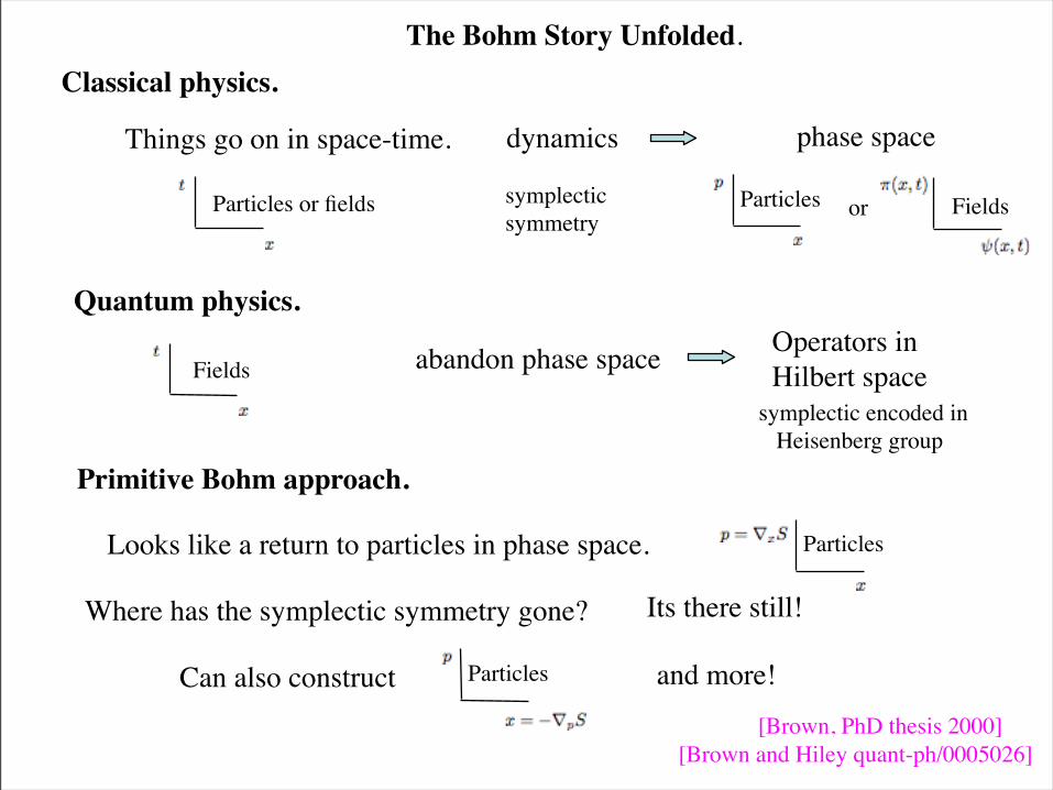
The Bohm Story Unfolded.Classical physics.

Quantum physics.

Things go on in space-time. dynamics phase space

Primitive Bohm approach.

Looks like a return to particles in phase space.

Particles or fields Particles Fieldsorsymplectic symmetry

Fields abandon phase space Operators in Hilbert space

symplectic encoded in Heisenberg group

Where has the symplectic symmetry gone? Its there still!

Particles

ParticlesCan also construct and more!

[Brown, PhD thesis 2000][Brown and Hiley quant-ph/0005026]

Non-commutativeAlgebraic structure.

Implicate order.

Holomovement

Possible explicate orders.

[D. Bohm Wholeness and the Implicate Order (1980])

The Overarching Structure

Process, activity

Shadowphase space

Shadowphase space

Shadowphase space

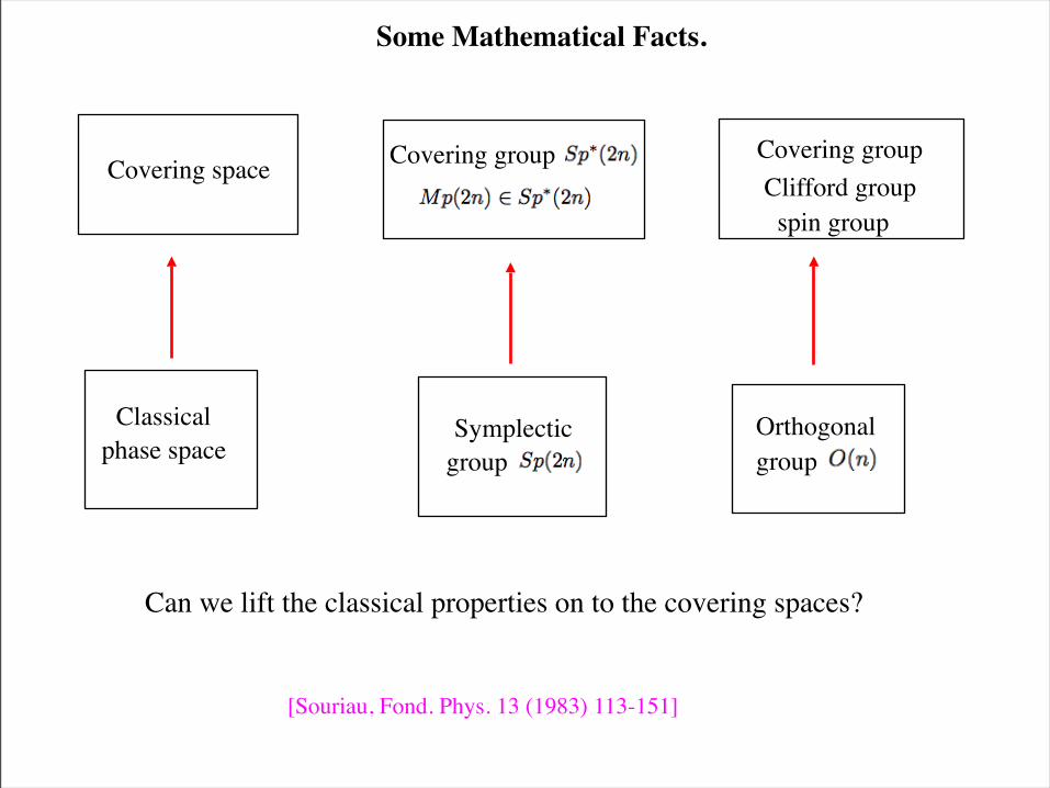
Can we lift the classical properties on to the covering spaces?

Classicalphase space

Covering space Covering group

Symplectic group

Orthogonalgroup

Covering groupClifford group spin group

Some Mathematical Facts.

[Souriau, Fond. Phys. 13 (1983) 113-151]

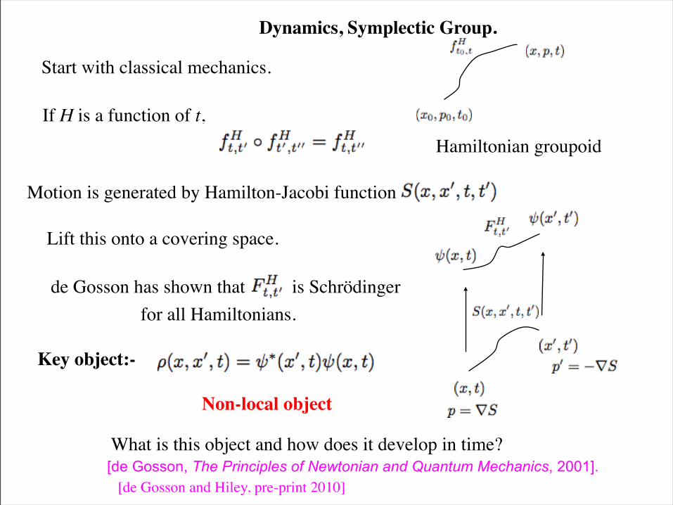
Dynamics, Symplectic Group.

Start with classical mechanics.

If H is a function of t,Hamiltonian groupoid

Motion is generated by Hamilton-Jacobi function

Lift this onto a covering space.

de Gosson has shown that is Schrödinger

What is this object and how does it develop in time?[de Gosson, The Principles of Newtonian and Quantum Mechanics, 2001].

for all Hamiltonians.

[de Gosson and Hiley, pre-print 2010]

Key object:-

Non-local object

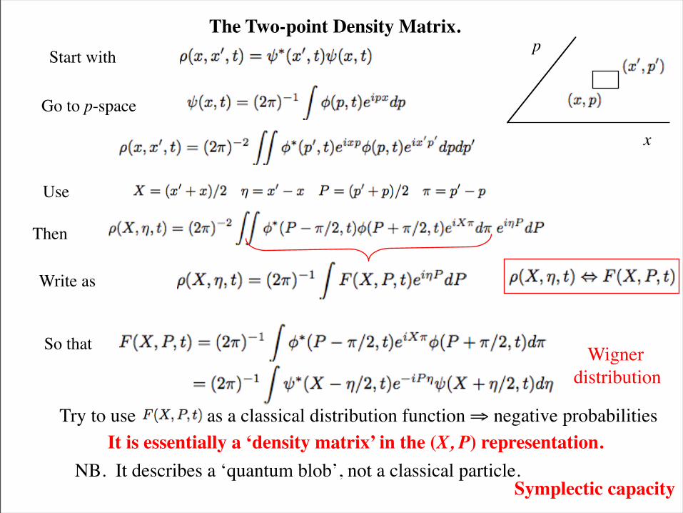
Start with

Use

Then

The Two-point Density Matrix.

x

p

(x1, p1)

(x2, p2)

So that

It is essentially a ‘density matrix’ in the (X, P) representation.

Wignerdistribution

Go to p-space

Write as

NB. It describes a ‘quantum blob’, not a classical particle.

Try to use as a classical distribution function ⇒ negative probabilities

Symplectic capacity

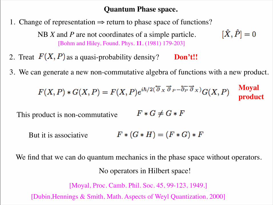
Quantum Phase space.1. Change of representation ⇒ return to phase space of functions?

NB X and P are not coordinates of a simple particle.

2. Treat as a quasi-probability density? Don’t!!

3. We can generate a new non-commutative algebra of functions with a new product.

[Dubin,Hennings & Smith, Math. Aspects of Weyl Quantization, 2000]

This product is non-commutative

But it is associative

We find that we can do quantum mechanics in the phase space without operators.

No operators in Hilbert space!

[Moyal, Proc. Camb. Phil. Soc. 45, 99-123, 1949.]

[Bohm and Hiley, Found. Phys. 11, (1981) 179-203]

Moyalproduct

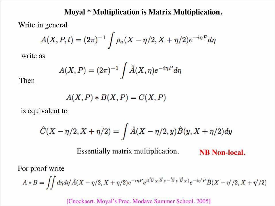
Moyal * Multiplication is Matrix Multiplication.Write in general

write as

Then

is equivalent to

Essentially matrix multiplication.

[Cnockaert, Moyal’s Proc. Modave Summer School, 2005]

For proof write

NB Non-local.

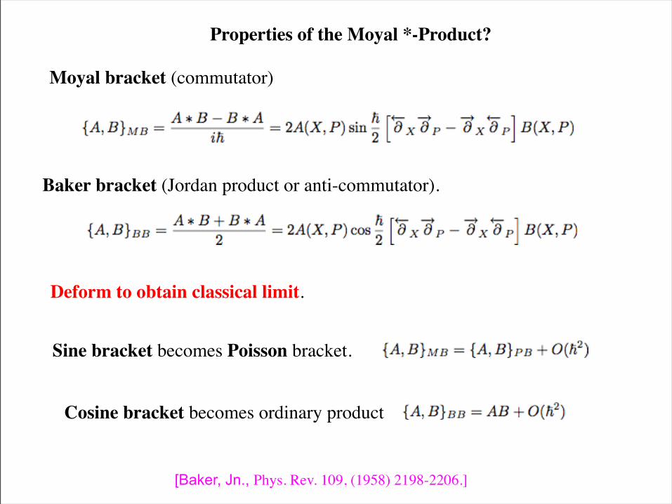
Moyal bracket (commutator)

Baker bracket (Jordan product or anti-commutator).

Properties of the Moyal *-Product?

Deform to obtain classical limit.

[Baker, Jn., Phys. Rev. 109, (1958) 2198-2206.]

Sine bracket becomes Poisson bracket.

Cosine bracket becomes ordinary product

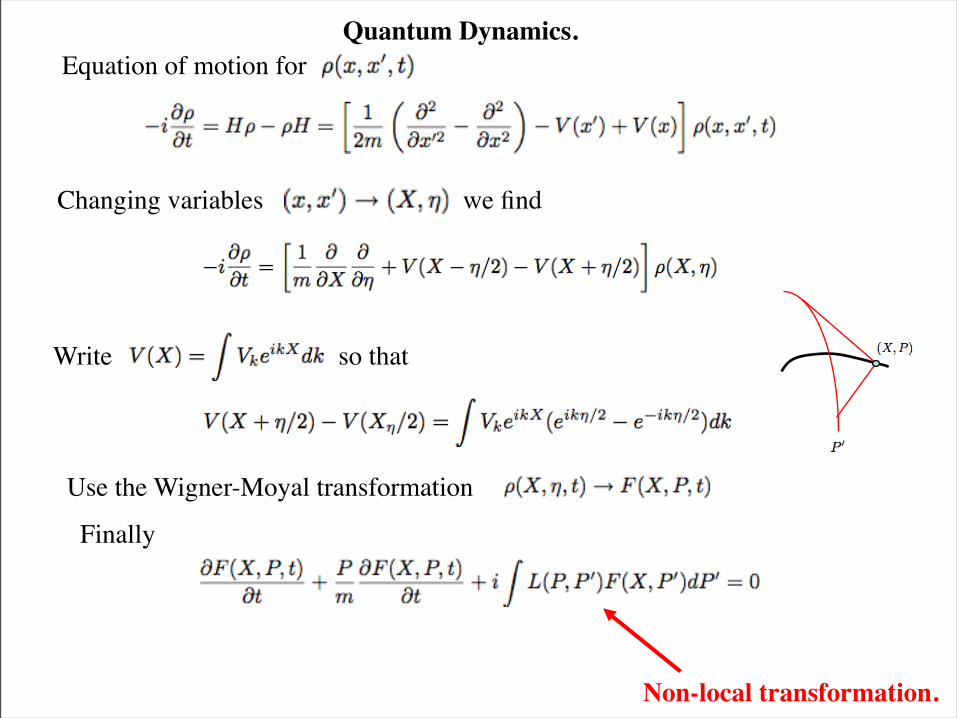
Quantum Dynamics.Equation of motion for

Changing variables we find

Write so that

Finally

Non-local transformation.

Use the Wigner-Moyal transformation

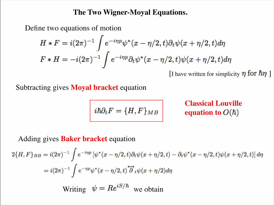
Define two equations of motion

Subtracting gives Moyal bracket equation

Adding gives Baker bracket equation

Classical Louvilleequation to

The Two Wigner-Moyal Equations.

[I have written for simplicity ]

Writing we obtain

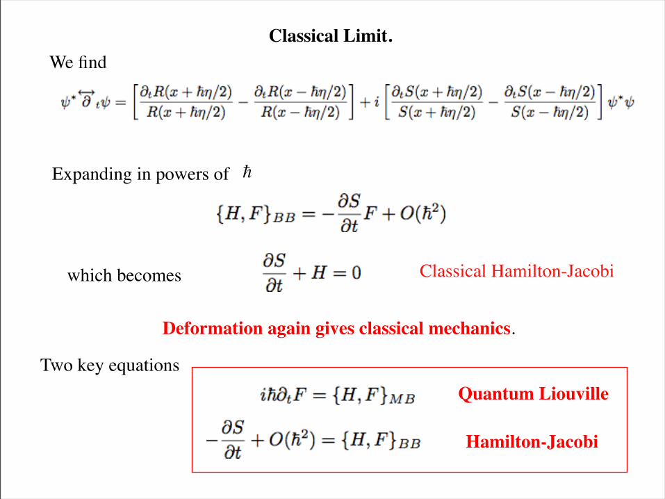
Classical Limit.We find

€

hExpanding in powers of

which becomes Classical Hamilton-Jacobi

Deformation again gives classical mechanics.

Two key equationsQuantum Liouville

Hamilton-Jacobi

Summary so far

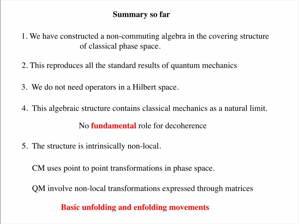
1. We have constructed a non-commuting algebra in the covering structure of classical phase space.

3. We do not need operators in a Hilbert space.

2. This reproduces all the standard results of quantum mechanics

4. This algebraic structure contains classical mechanics as a natural limit.

No fundamental role for decoherence

5. The structure is intrinsically non-local.

CM uses point to point transformations in phase space.

QM involve non-local transformations expressed through matrices

Basic unfolding and enfolding movements

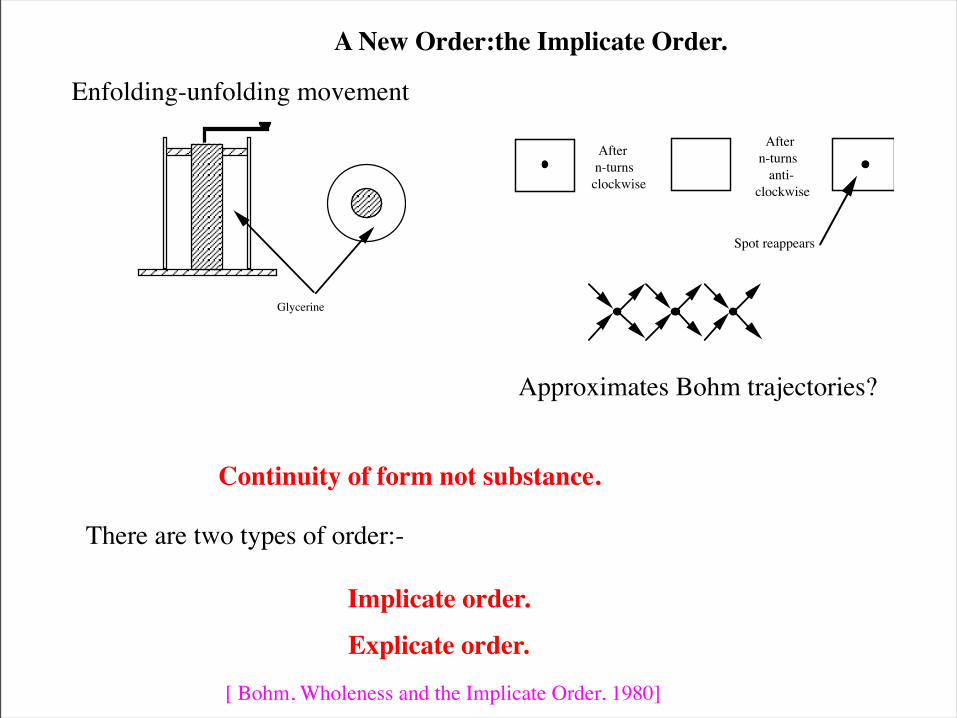
Glycerine

After n-turnsclockwise

After n-turns anti-clockwise

Spot reappears

Approximates Bohm trajectories?

Continuity of form not substance.

Enfolding-unfolding movement

There are two types of order:-

Implicate order.

Explicate order.

[ Bohm, Wholeness and the Implicate Order, 1980]

A New Order:the Implicate Order.

€

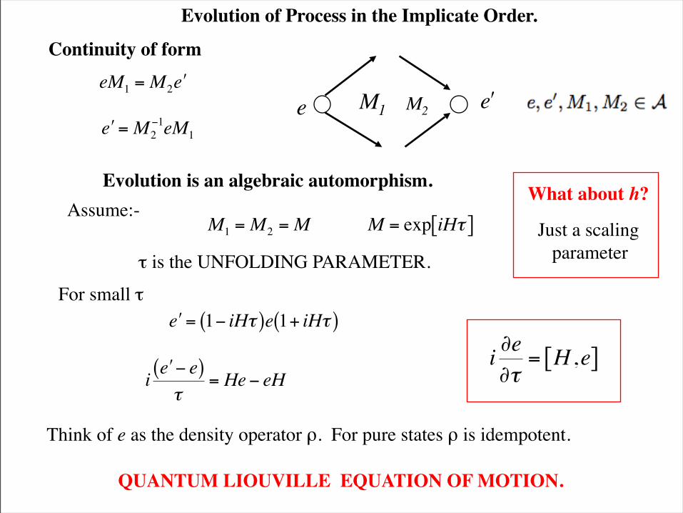
eM1 = M2 ′ e

€

′ e = M2−1eM1

e M1 M2

€

′ e

€

M1 = M2 = M M = exp iHτ[ ]

€

′ e = 1− iHτ( )e 1+ iHτ( )

€

i′ e − e( )τ

= He− eH

Continuity of form

Evolution is an algebraic automorphism.Assume:-

τ is the UNFOLDING PARAMETER.

For small τ

QUANTUM LIOUVILLE EQUATION OF MOTION.€

i ∂e∂τ

= H ,e[ ]

Think of e as the density operator ρ. For pure states ρ is idempotent.

What about h?

Just a scaling parameter

Evolution of Process in the Implicate Order.

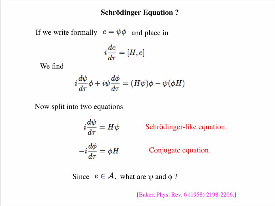
Schrödinger Equation ?

We find

Now split into two equations

If we write formally and place in

Schrödinger-like equation.

Conjugate equation.

Since , what are ψ and φ ?

[Baker, Phys. Rev. 6 (1958) 2198-2206.]

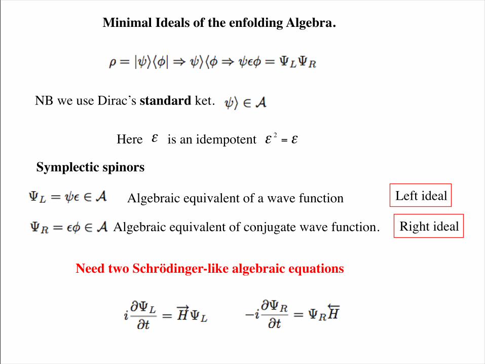
ε ε 2 = εHere is an idempotent

Symplectic spinors

Need two Schrödinger-like algebraic equations

Minimal Ideals of the enfolding Algebra.

NB we use Dirac’s standard ket.

Left idealAlgebraic equivalent of a wave function

Right idealAlgebraic equivalent of conjugate wave function.

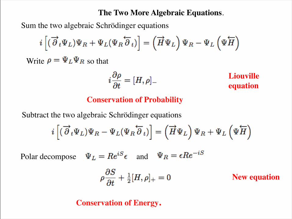
Sum the two algebraic Schrödinger equations

Conservation of Probability

Subtract the two algebraic Schrödinger equations

Conservation of Energy.

New equation

Liouvilleequation

The Two More Algebraic Equations.

Write so that

Polar decompose and

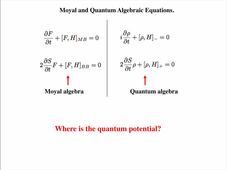
Moyal algebra Quantum algebra

Where is the quantum potential?

Moyal and Quantum Algebraic Equations.

€

ˆ H = ˆ p 2

2m+

Kˆ x 2

2

€

∂Sx

∂t+12m

∂Sx

∂x

2

+Kx 2

2−

12mRx

∂2Rx

∂x 2

= 0

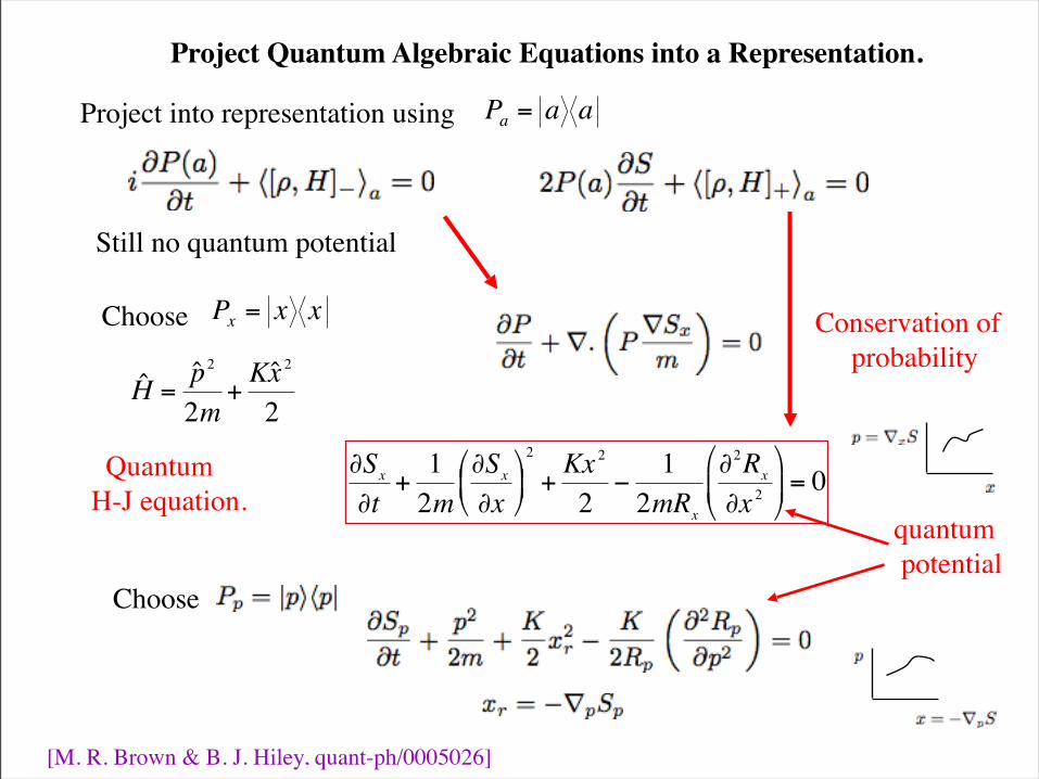
Project into representation using

€

Pa = a a

Still no quantum potential

Choose

€

Px = x x Conservation of probability

Quantum H-J equation.

quantum potential

[M. R. Brown & B. J. Hiley, quant-ph/0005026]

Project Quantum Algebraic Equations into a Representation.

Choose

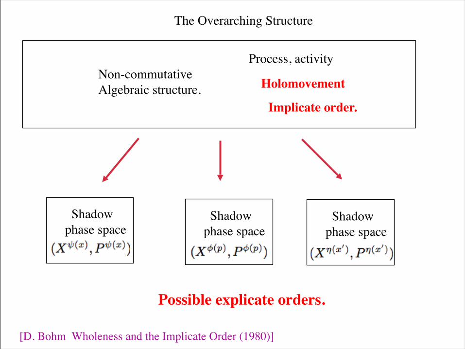
Non-commutativeAlgebraic structure.

Implicate order.

Holomovement

Possible explicate orders.

[D. Bohm Wholeness and the Implicate Order (1980)]

The Overarching Structure

Process, activity

Shadowphase space

Shadowphase space

Shadowphase space

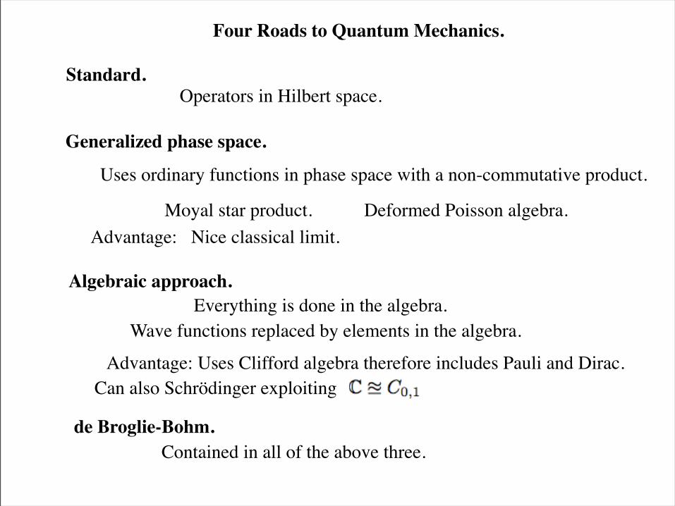
Four Roads to Quantum Mechanics.

Standard.Operators in Hilbert space.

Generalized phase space.

Uses ordinary functions in phase space with a non-commutative product.

Moyal star product. Deformed Poisson algebra.Advantage: Nice classical limit.

Algebraic approach.Everything is done in the algebra.

Wave functions replaced by elements in the algebra.

Advantage: Uses Clifford algebra therefore includes Pauli and Dirac.Can also Schrödinger exploiting

de Broglie-Bohm.Contained in all of the above three.

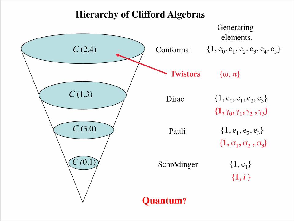
Hierarchy of Clifford Algebras

C (0,1)

C (3,0)

C (1,3)

C (2,4) Conformal

Dirac

Pauli

Schrödinger

{1, e1, e2, e3}

{1, e1}

{1, e0, e1, e2, e3}

{1, e0, e1, e2, e3, e4, e5}

Generating elements.

Quantum?

Twistors

{1, i }

{1, σ1, σ2 , σ3}

{1, γ0, γ1, γ2 , γ3}

{ω, π}

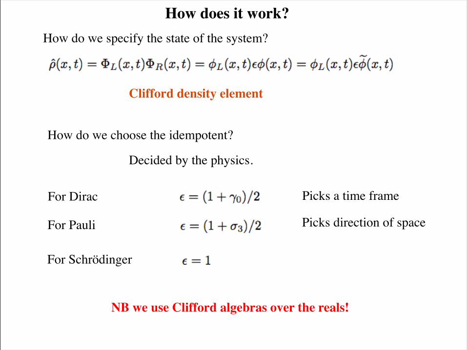
How does it work?How do we specify the state of the system?

Clifford density element

How do we choose the idempotent?

Decided by the physics.

For Schrödinger

For Pauli Picks direction of space

For Dirac Picks a time frame

NB we use Clifford algebras over the reals!

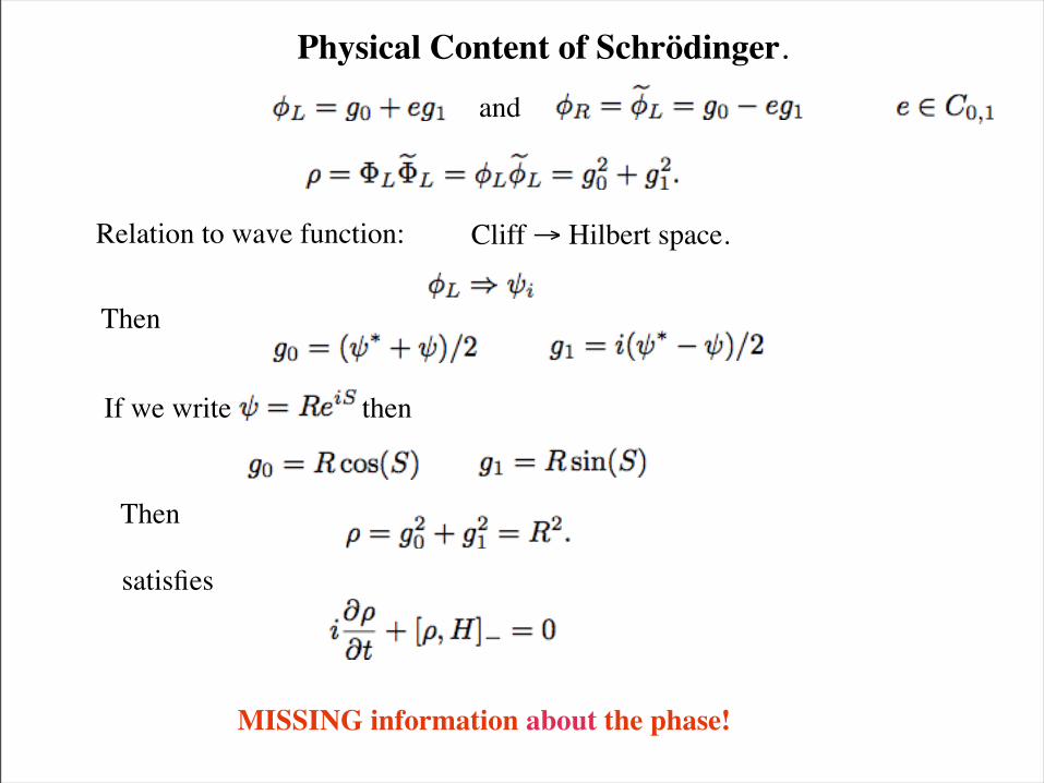
Physical Content of Schrödinger.

Then

MISSING information about the phase!

and

Relation to wave function: Cliff → Hilbert space.

Then

satisfies

If we write then

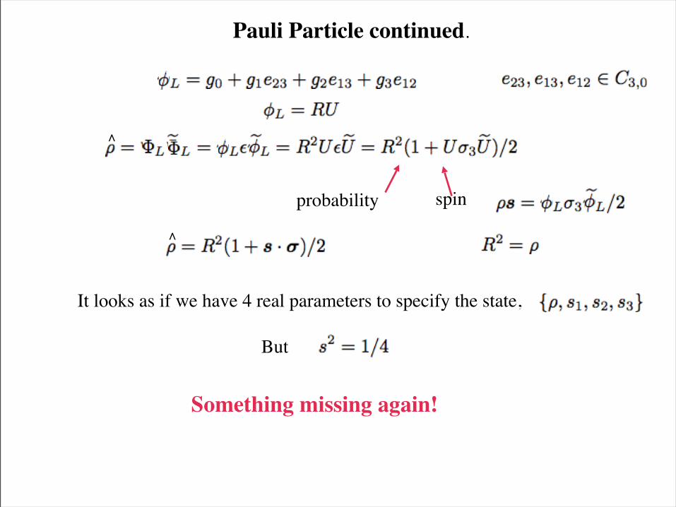
Pauli Particle continued.

It looks as if we have 4 real parameters to specify the state,

But

Something missing again!

probability spin

∧

∧

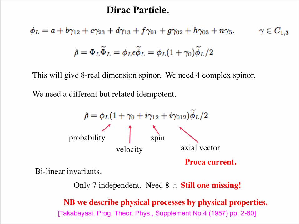
Dirac Particle.

This will give 8-real dimension spinor. We need 4 complex spinor.

We need a different but related idempotent.

probabilityvelocity

spinaxial vector

Proca current.Bi-linear invariants.

Only 7 independent. Need 8 ∴ Still one missing!

NB we describe physical processes by physical properties.[Takabayasi, Prog. Theor. Phys., Supplement No.4 (1957) pp. 2-80]

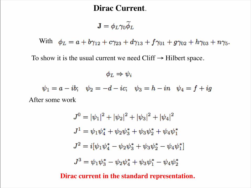
Dirac Current.

To show it is the usual current we need Cliff → Hilbert space.

After some work

Dirac current in the standard representation.

With

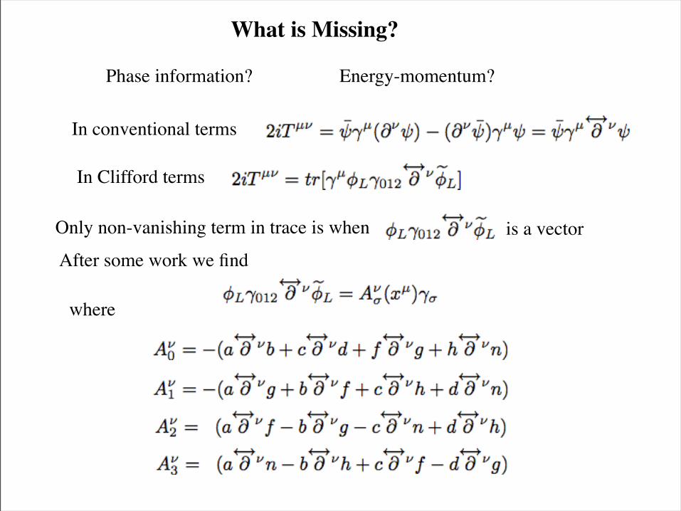
What is Missing?

Phase information? Energy-momentum?

In conventional terms

After some work we find

where

Only non-vanishing term in trace is when is a vector

In Clifford terms

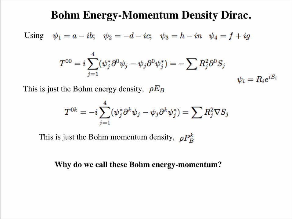
Bohm Energy-Momentum Density Dirac.Using

This is just the Bohm momentum density,

This is just the Bohm energy density,

Why do we call these Bohm energy-momentum?

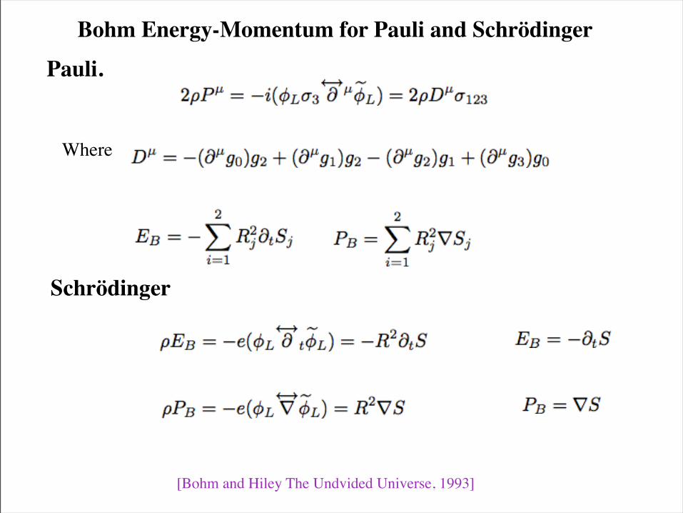
Bohm Energy-Momentum for Pauli and Schrödinger

Pauli.

Where

Schrödinger

[Bohm and Hiley The Undvided Universe, 1993]

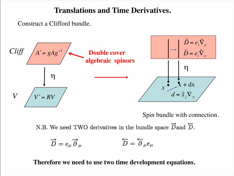
Translations and Time Derivatives.

Double cover algebraic spinors

Spin bundle with connection.

V

Cliff

η €

′ A = gAg−1

€

′ V = RV

€

r D = ei

r ∇ ei

€

s D = ei

s ∇ ei

x x + dx

€

d = ˆ x j∇ x j

η

Construct a Clifford bundle.

Therefore we need to use two time development equations.

and

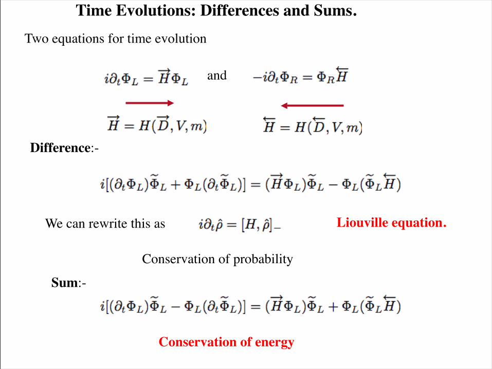
Time Evolutions: Differences and Sums.

Difference:-

We can rewrite this as Liouville equation.

Sum:-

Conservation of probability

Conservation of energy

Two equations for time evolution

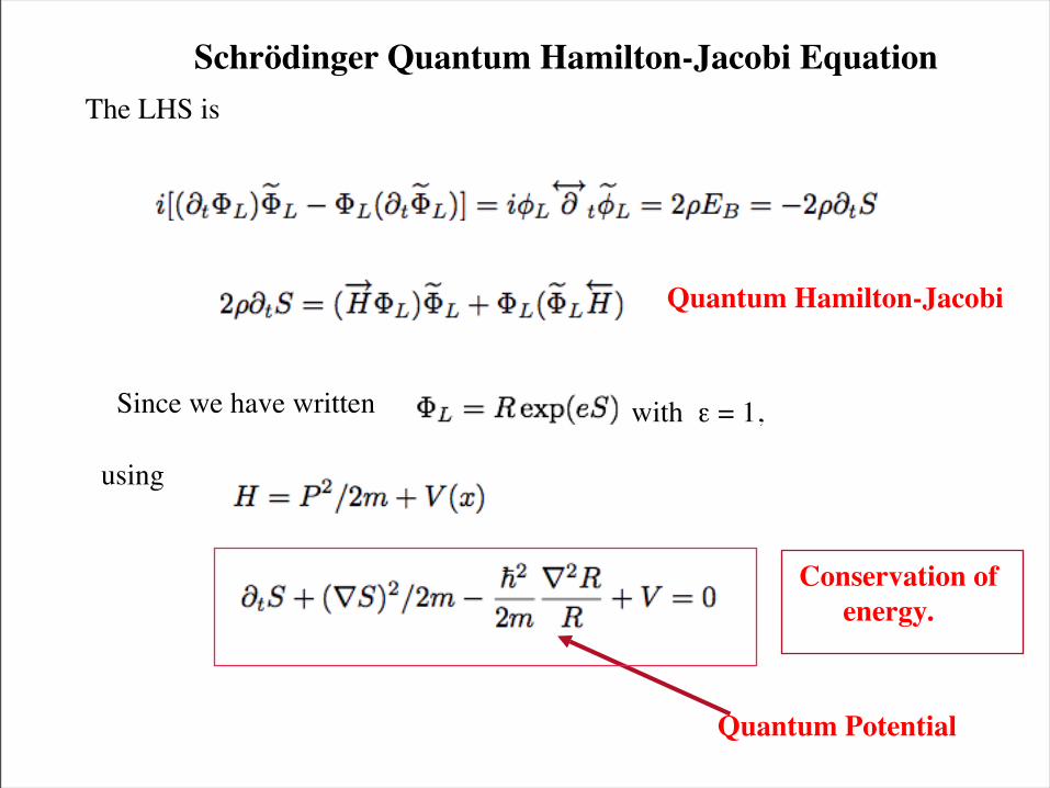
The LHS is

Quantum Hamilton-Jacobi

Since we have written with ε = 1,

using

Quantum Potential

Conservation of energy.

Schrödinger Quantum Hamilton-Jacobi Equation

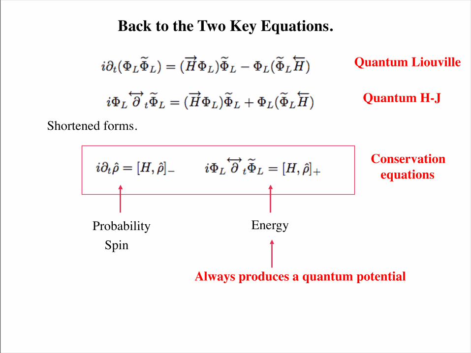
Back to the Two Key Equations.

Shortened forms.

ProbabilitySpin

Energy

Conservation equations

Always produces a quantum potential

Quantum Liouville

Quantum H-J

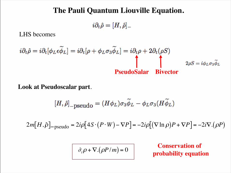
The Pauli Quantum Liouville Equation.

LHS becomes

€

2m H , ˆ ρ [ ]−pseudo = 2iρ 4S ⋅ P ⋅W( )−∇P[ ] = −2iρ ∇ lnρ( )P+∇P[ ] = −2i∇. ρP( )

€

∂tρ +∇. ρP /m( ) = 0 Conservation of probability equation

Look at Pseudoscalar part.

PseudoSalar Bivector

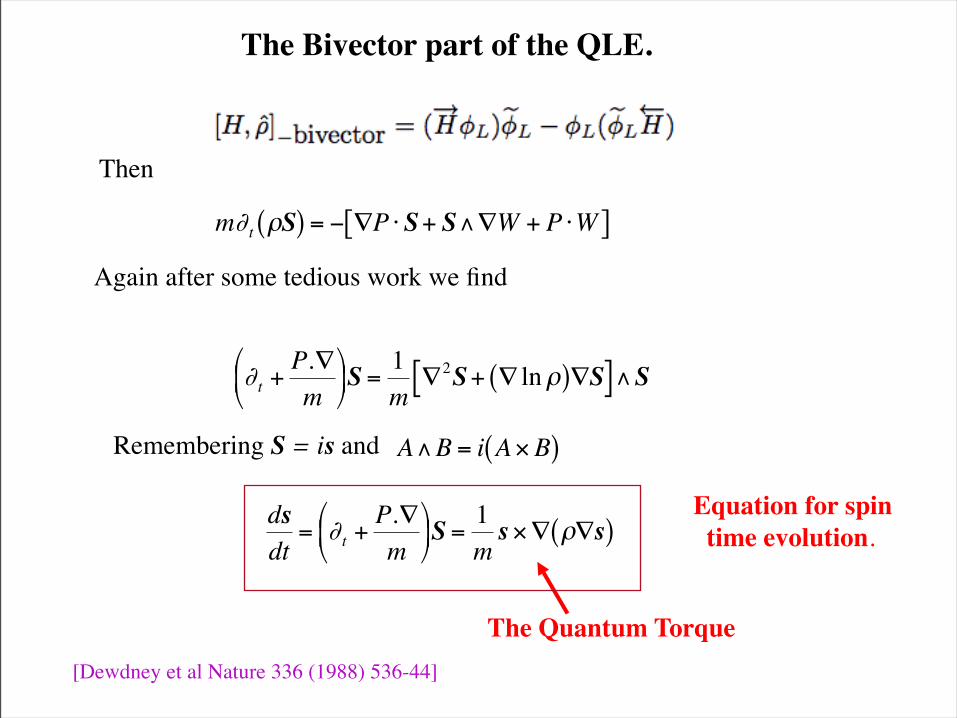
The Bivector part of the QLE.

Then

€

m∂t ρS( ) = − ∇P ⋅ S+ S∧∇W + P ⋅W[ ]

Again after some tedious work we find

€

∂t +P.∇m

S =

1m

∇2S+ ∇ lnρ( )∇S[ ]∧S

Remembering S = is and

€

A∧B = i A×B( )

€

dsdt

= ∂t +P.∇m

S =

1ms×∇ ρ∇s( )

Equation for spin time evolution.

The Quantum Torque[Dewdney et al Nature 336 (1988) 536-44]

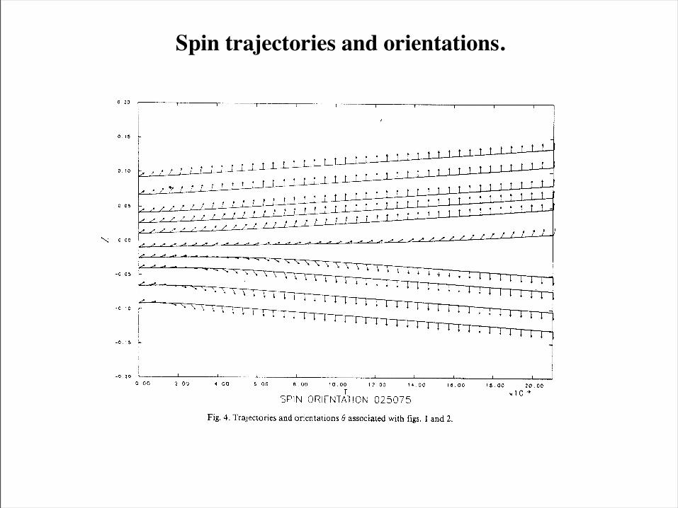
Spin trajectories and orientations.

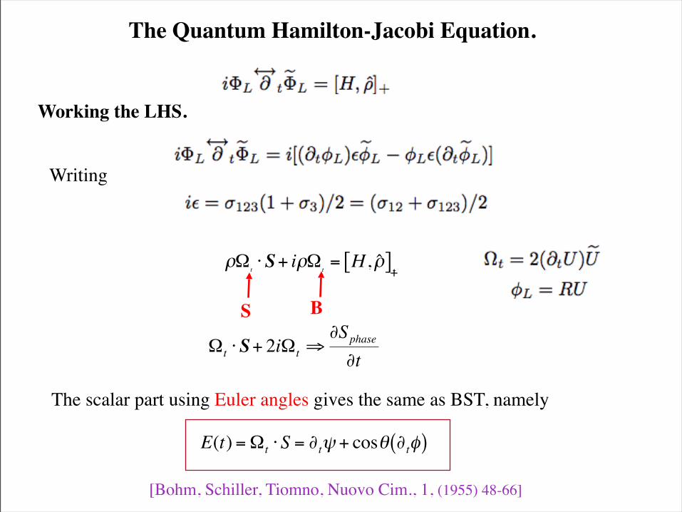
The Quantum Hamilton-Jacobi Equation.

S B

€

Ωt ⋅ S+ 2iΩt ⇒∂Sphase∂t

The scalar part using Euler angles gives the same as BST, namely

€

E(t) =Ωt ⋅S = ∂tψ + cosθ ∂tφ( )

Writing

Working the LHS.

[Bohm, Schiller, Tiomno, Nuovo Cim., 1, (1955) 48-66]

€

ρΩt⋅ S+ iρΩ

t= H , ˆ ρ [ ]

++

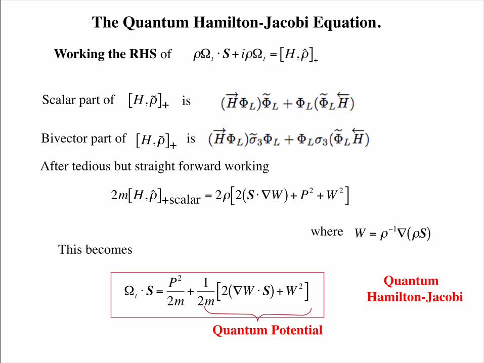
The Quantum Hamilton-Jacobi Equation.

where

€

W = ρ−1∇ ρS( )

€

ρΩt ⋅ S+ iρΩt = H , ˆ ρ [ ]+Working the RHS of

Scalar part of

€

H , ˜ ρ [ ]+

€

H , ˜ ρ [ ]+

is

Bivector part of is

After tedious but straight forward working

€

2m H , ˆ ρ [ ]+scalar = 2ρ 2 S ⋅ ∇W( ) + P2 +W 2[ ]

This becomes

€

Ωt ⋅ S =P2

2m+12m

2 ∇W ⋅ S( ) +W 2[ ] QuantumHamilton-Jacobi

Quantum Potential

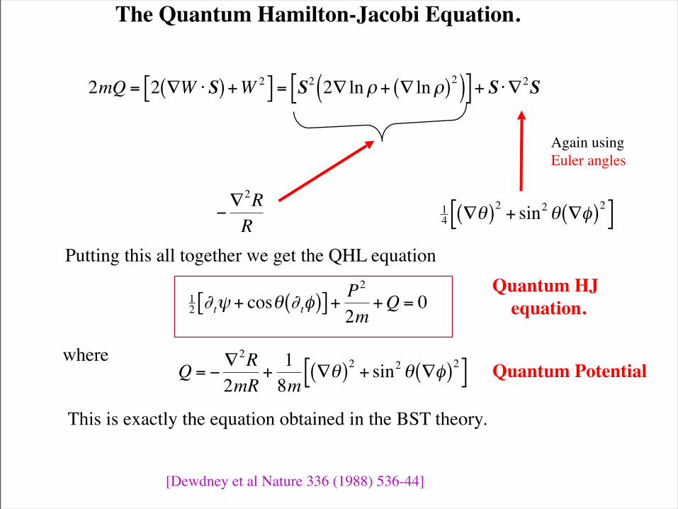
The Quantum Hamilton-Jacobi Equation.

€

2mQ = 2 ∇W ⋅ S( ) +W 2[ ] = S2 2∇ lnρ + ∇ lnρ( )2( )[ ] + S ⋅ ∇2S

€

−∇2RR

€

14 ∇θ( )2 + sin2θ ∇φ( )2[ ]

Putting this all together we get the QHL equation

€

12 ∂tψ + cosθ ∂tφ( )[ ] +

P2

2m+Q = 0

where

€

Q = −∇2R2mR

+18m

∇θ( )2 + sin2θ ∇φ( )2[ ]This is exactly the equation obtained in the BST theory.

[Dewdney et al Nature 336 (1988) 536-44]

Quantum Potential

Quantum HJ equation.

Again usingEuler angles

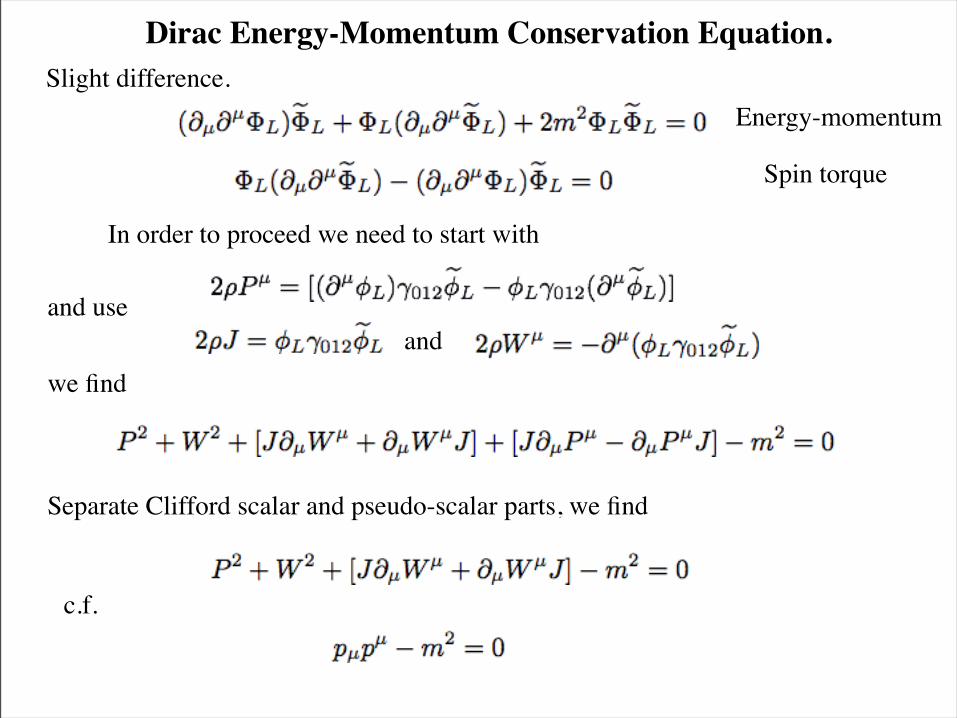
Dirac Energy-Momentum Conservation Equation.Slight difference.

Energy-momentum

Spin torque

In order to proceed we need to start with

and use

we find

Separate Clifford scalar and pseudo-scalar parts, we find

c.f.

and

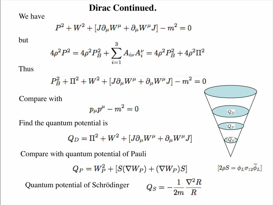
Dirac Continued.We have

but

Thus

Compare with

Find the quantum potential is

Compare with quantum potential of Pauli

Quantum potential of Schrödinger

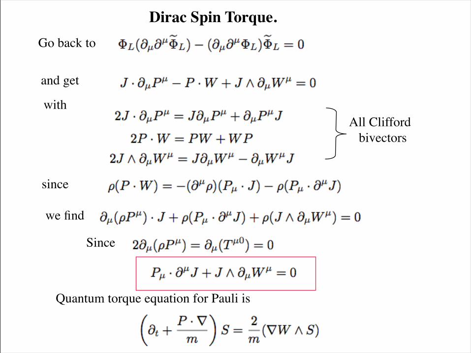
Dirac Spin Torque.

and get

withAll Clifford bivectors

since

we find

Since

Quantum torque equation for Pauli is

Go back to

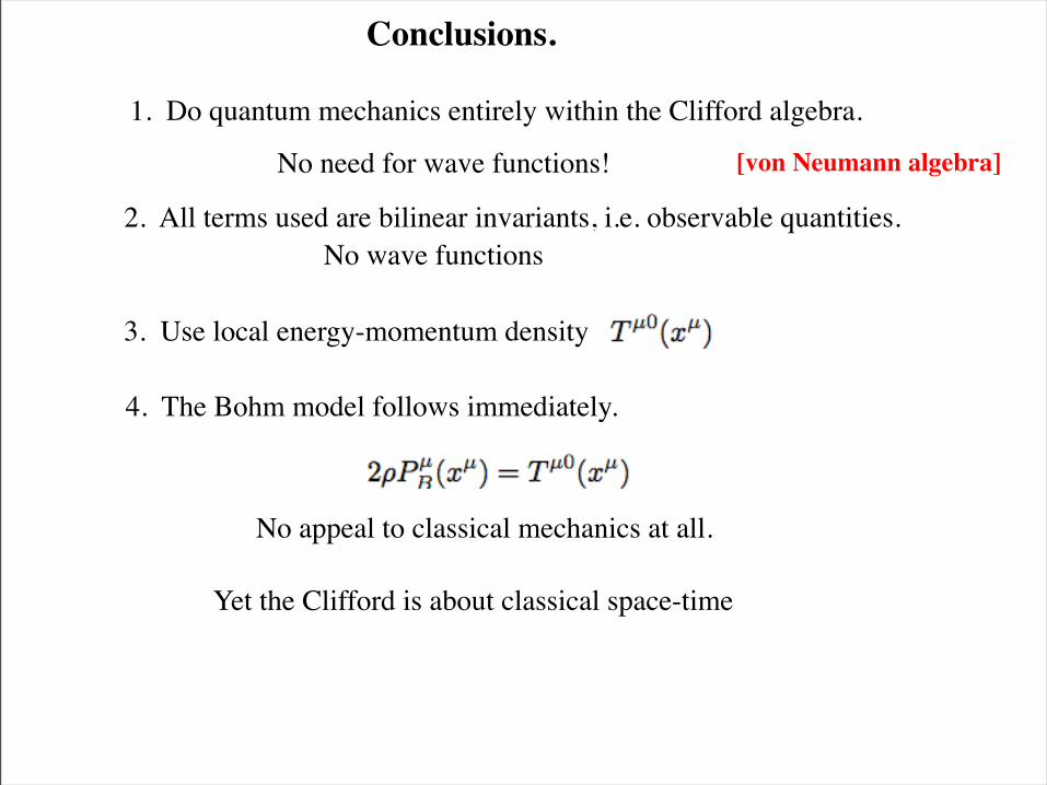
Conclusions.

1. Do quantum mechanics entirely within the Clifford algebra.

No need for wave functions!

2. All terms used are bilinear invariants, i.e. observable quantities.

4. The Bohm model follows immediately.

No appeal to classical mechanics at all.

3. Use local energy-momentum density

[von Neumann algebra]

Yet the Clifford is about classical space-time

No wave functions

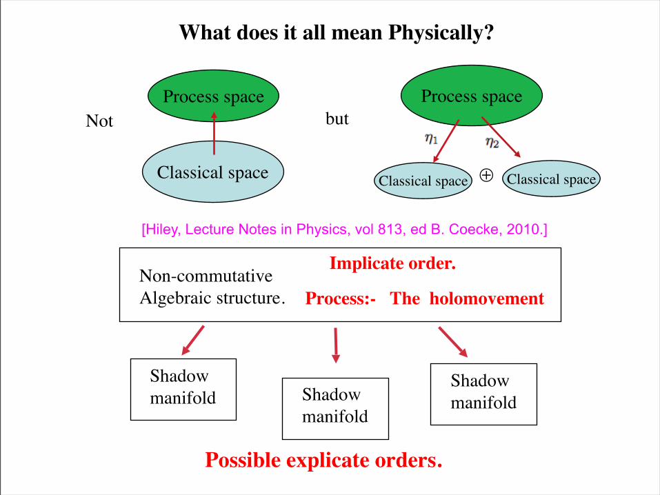
What does it all mean Physically?

Non-commutativeAlgebraic structure.

Implicate order.

Process:- The holomovement

Shadowmanifold

Possible explicate orders.

ShadowmanifoldShadow

manifold

Classical space

Process space Process spaceNot but

Classical spaceClassical space ⊕

[Hiley, Lecture Notes in Physics, vol 813, ed B. Coecke, 2010.]

References.Frescura, F. A. M. and Hiley, B. J., The Implicate Order, Algebras, and the Spinor, Found. Phys. 10, (1980), 7-31.

Frescura, F. A. M. and Hiley, B. J., (1984) Algebras, Quantum Theory and Pre-Space, Revista Brasilera de Fisica, Volume Especial, Os 70 anos de Mario Schonberg, 49-86.

Bohm, D., and Hiley, B. J., Generalization of the Twistor to Clifford Algebras as a basis for Geometry, Rev. Briasileira de Fisica, Volume Especial, Os 70 anos de Mario Schonberg, (1984) 1-26

Hestenes, D., and Gurtler, R., Local Observables in Quantum Theory, Am. J. Phys. 39, (1971) 1028-38.

Hiley, B. J., Non-commutative Quantum Geometry: a re-appraisal of the Bohm approach to quantum theory, Quo Vadis Quantum Mechanics, ed Elitzur, A., Dolev, S., and Kolenda, N., 299-324, Springer, Berlin (2005)

Hiley, B. J., Process, Distinction, Groupoids and Clifford Algebras: an Alternative View of the Quantum Formalism, Collection of Essays, ed., Coecke, B. (2009)

Hiley, B. J., and Callaghan, R. E., The Clifford Algebra approach to Quantum Mechanics A: The Schr\"{o}dinger and Pauli Particles.B: The Dirac Particle and its relation to the Bohm Approach, Pre-prints, (2009)