James Gayvert1, Alexandros Chremos2, Jack Douglas2

1Le Moyne College, 2National Institute of Standards and Technology(NIST), U.S. Department of Commerce, Gaithersburg, Maryland, USA

Molecular Dynamics Study of the Conformational Properties of Polymers

in an Explicit Solvent and the Identification of the θ-Temperature

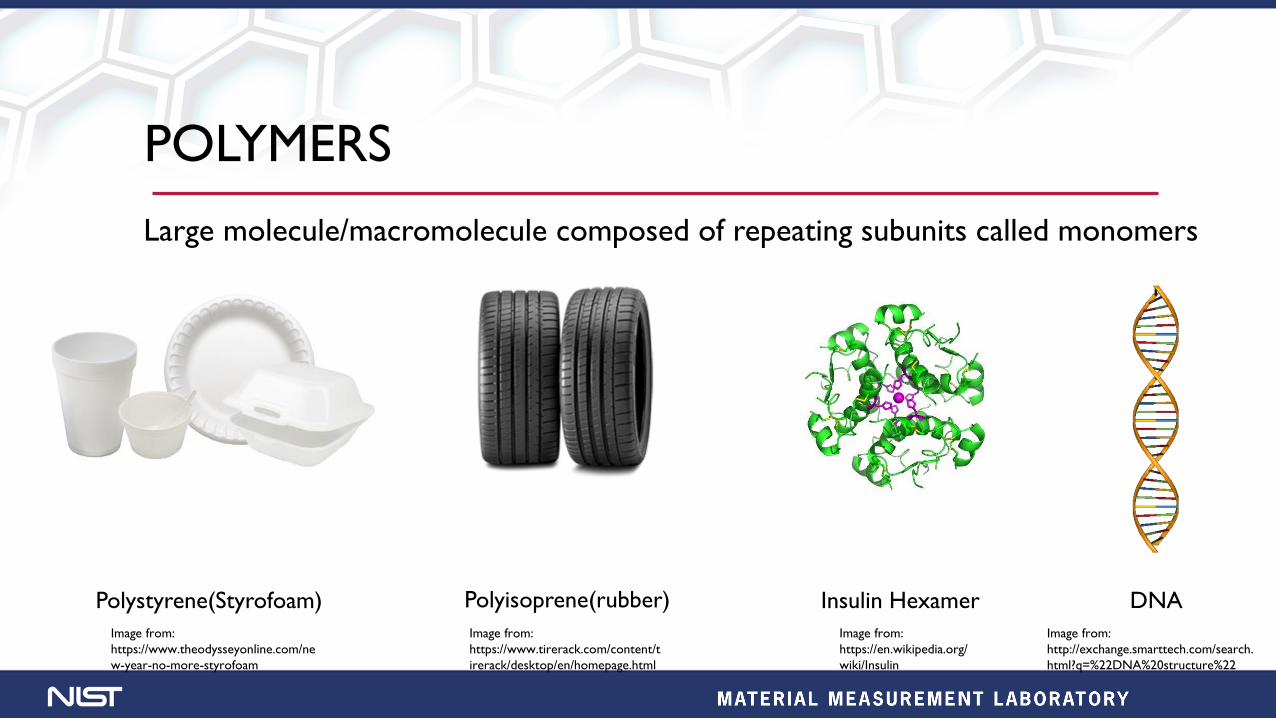
POLYMERS

Large molecule/macromolecule composed of repeating subunits called monomers

Polystyrene(Styrofoam) Polyisoprene(rubber) Insulin Hexamer DNA

Image from:

https://www.theodysseyonline.com/ne

w-year-no-more-styrofoam

Image from:

https://www.tirerack.com/content/t

irerack/desktop/en/homepage.html

Image from:

https://en.wikipedia.org/

wiki/Insulin

Image from:

http://exchange.smarttech.com/search.

html?q=%22DNA%20structure%22

POLYMER MODELS

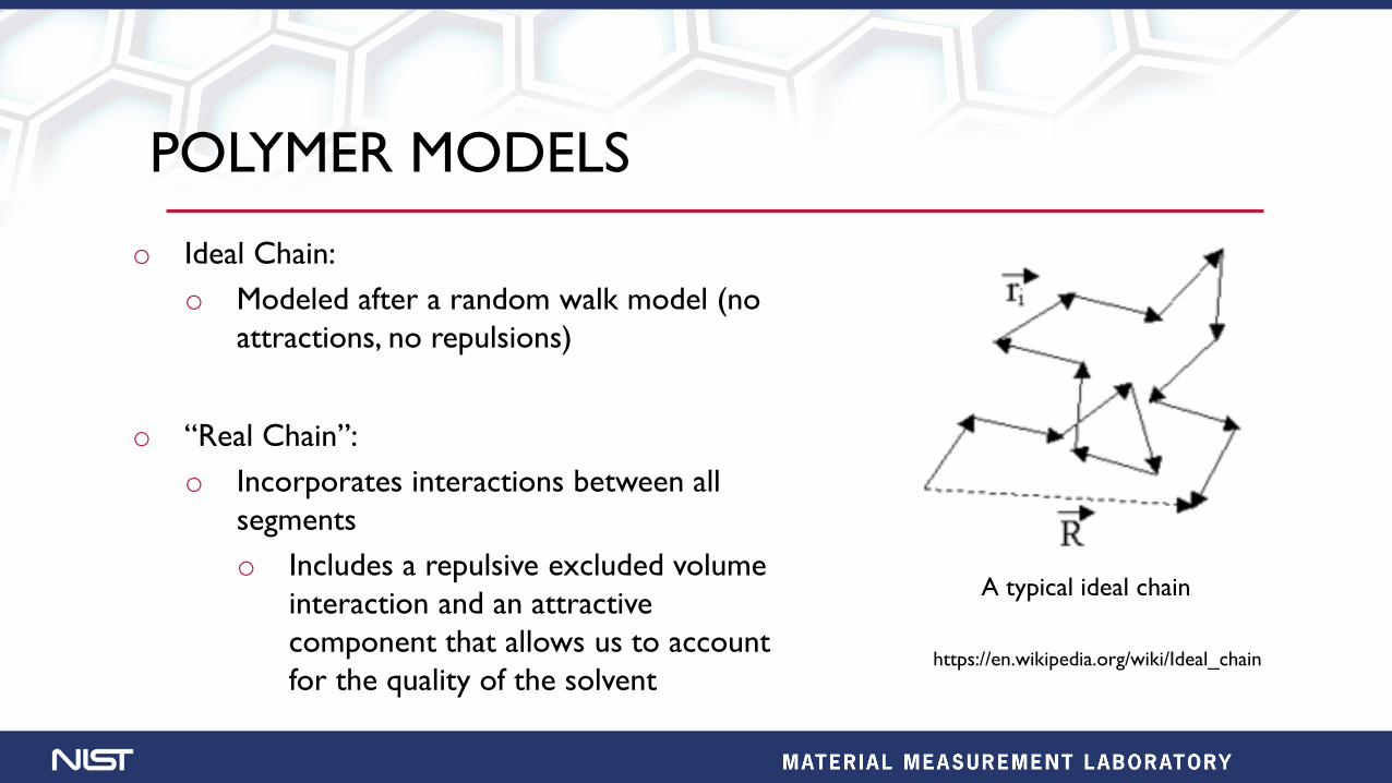
o Ideal Chain:

o Modeled after a random walk model (no

attractions, no repulsions)

o “Real Chain”:

o Incorporates interactions between all

segments

o Includes a repulsive excluded volume

interaction and an attractive

component that allows us to account

for the quality of the solvent

A typical ideal chain

https://en.wikipedia.org/wiki/Ideal_chain

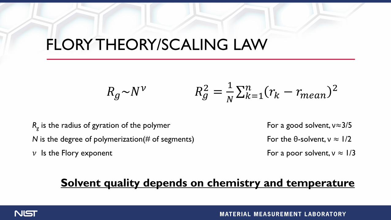
FLORY THEORY/SCALING LAW

𝑅𝑔~𝑁𝜈 𝑅𝑔

2 =1

𝑁σ𝑘=1𝑛 𝑟𝑘 − 𝑟𝑚𝑒𝑎𝑛

2

Rg is the radius of gyration of the polymer For a good solvent, ν≈3/5

N is the degree of polymerization(# of segments) For the θ-solvent, ν ≈ 1/2

𝜈 Is the Flory exponent For a poor solvent, ν ≈ 1/3

Solvent quality depends on chemistry and temperature

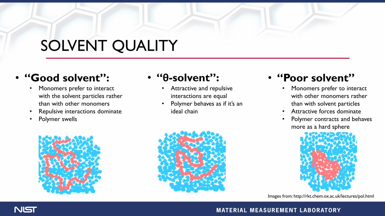
SOLVENT QUALITY

• “Good solvent”:• Monomers prefer to interact

with the solvent particles rather

than with other monomers

• Repulsive interactions dominate

• Polymer swells

• “θ-solvent”:• Attractive and repulsive

interactions are equal

• Polymer behaves as if it’s an

ideal chain

• “Poor solvent”• Monomers prefer to interact

with other monomers rather

than with solvent particles

• Attractive forces dominate

• Polymer contracts and behaves

more as a hard sphere

Images from: http://rkt.chem.ox.ac.uk/lectures/pol.html

OBJECTIVES

• Develop a model that can identify the θ-temperature

of a polymer solution

• Use molecular dynamics to simulate polymers of

varying chemistries and molecular architectures in an

explicit solvent

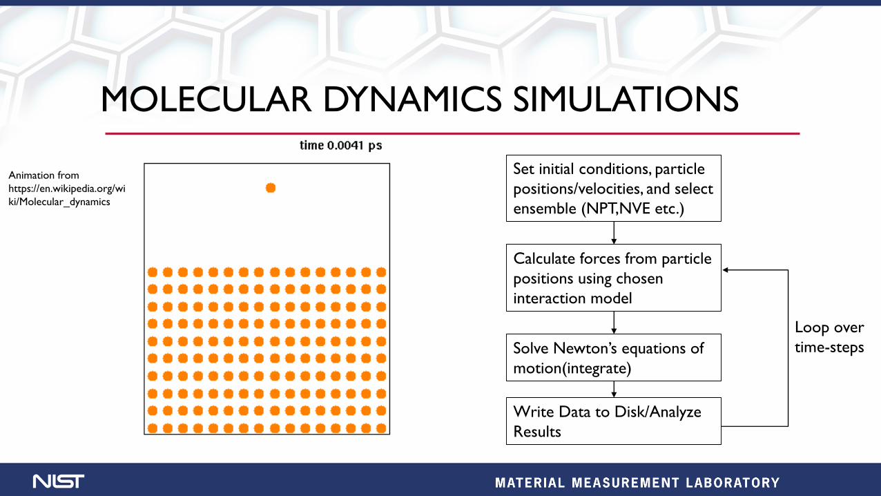
MOLECULAR DYNAMICS SIMULATIONS

Set initial conditions, particle

positions/velocities, and select

ensemble (NPT,NVE etc.)

Calculate forces from particle

positions using chosen

interaction model

Solve Newton’s equations of

motion(integrate)

Write Data to Disk/Analyze

Results

Loop over

time-steps

Animation from

https://en.wikipedia.org/wi

ki/Molecular_dynamics

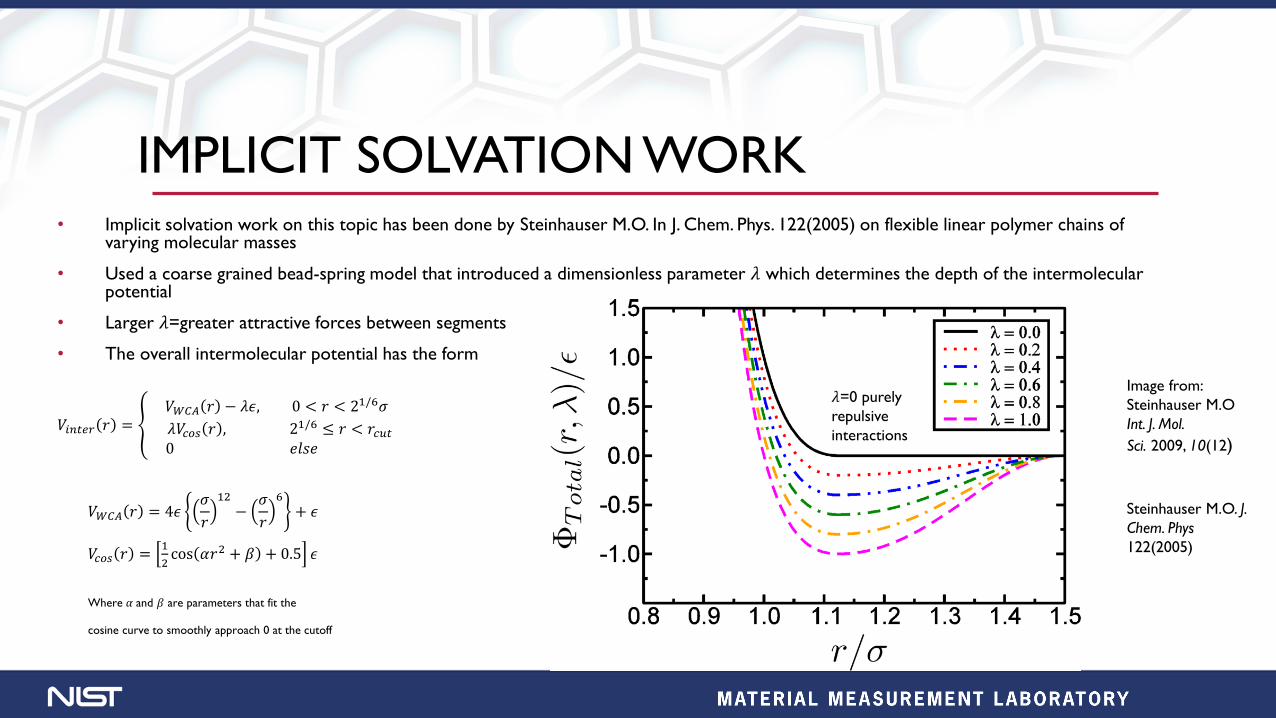
IMPLICIT SOLVATION WORK• Implicit solvation work on this topic has been done by Steinhauser M.O. In J. Chem. Phys. 122(2005) on flexible linear polymer chains of

varying molecular masses

• Used a coarse grained bead-spring model that introduced a dimensionless parameter 𝜆 which determines the depth of the intermolecular potential

• Larger 𝜆=greater attractive forces between segments

• The overall intermolecular potential has the form

𝑉𝑖𝑛𝑡𝑒𝑟 𝑟 = ൞𝑉𝑊𝐶𝐴 𝑟 − 𝜆𝜖, 0 < 𝑟 < 21/6𝜎

𝜆𝑉𝑐𝑜𝑠 𝑟 , 21/6 ≤ 𝑟 < 𝑟𝑐𝑢𝑡0 𝑒𝑙𝑠𝑒

𝑉𝑊𝐶𝐴 𝑟 = 4𝜖𝜎

𝑟

12

−𝜎

𝑟

6

+ 𝜖

𝑉𝑐𝑜𝑠 𝑟 =1

2cos 𝛼𝑟2 + 𝛽 + 0.5 𝜖

Where 𝛼 and 𝛽 are parameters that fit the

cosine curve to smoothly approach 0 at the cutoff

Image from:

Steinhauser M.O

Int. J. Mol.

Sci. 2009, 10(12)

Steinhauser M.O. J.

Chem. Phys

122(2005)

𝜆=0 purely

repulsive

interactions

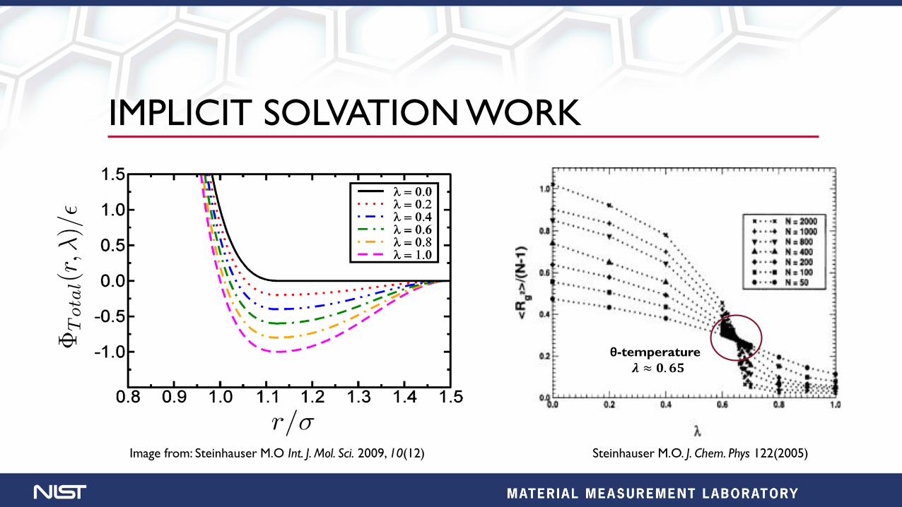
IMPLICIT SOLVATION WORK

Image from: Steinhauser M.O Int. J. Mol. Sci. 2009, 10(12) Steinhauser M.O. J. Chem. Phys 122(2005)

θ-temperature

𝝀 ≈ 𝟎. 𝟔𝟓

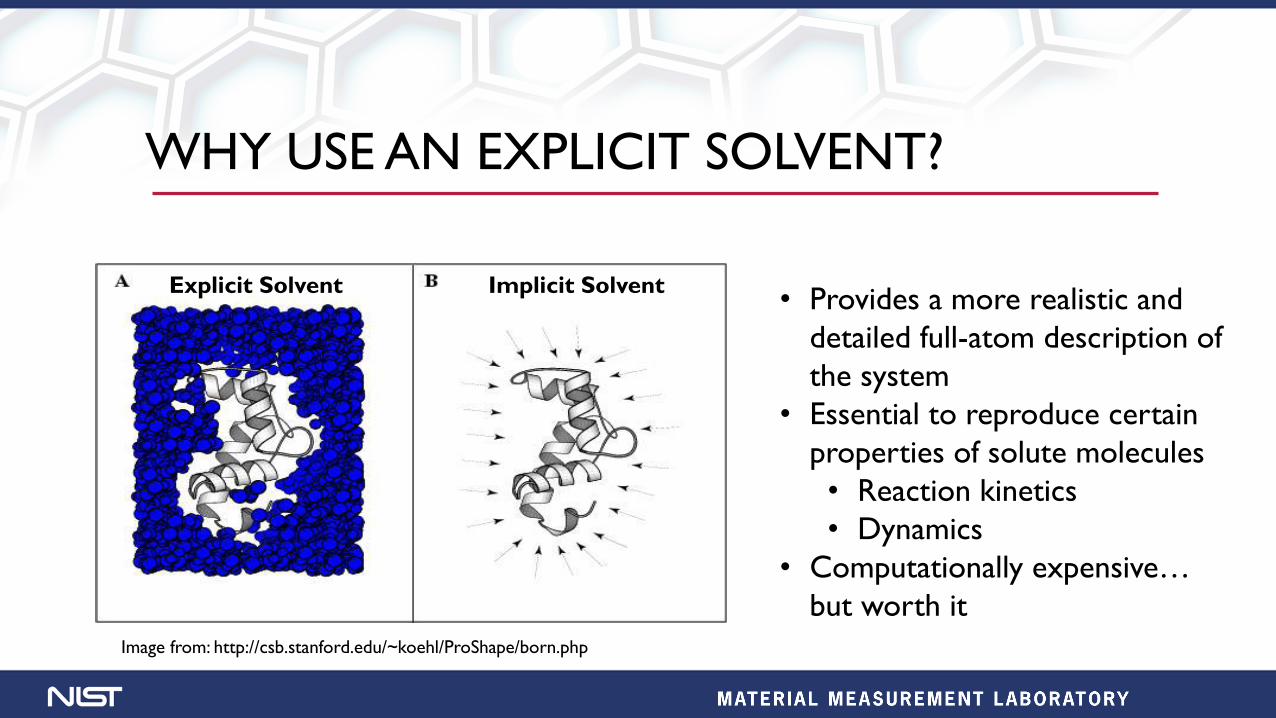
WHY USE AN EXPLICIT SOLVENT?

Explicit Solvent Implicit Solvent• Provides a more realistic and

detailed full-atom description of

the system

• Essential to reproduce certain

properties of solute molecules

• Reaction kinetics

• Dynamics

• Computationally expensive…

but worth it

Image from: http://csb.stanford.edu/~koehl/ProShape/born.php

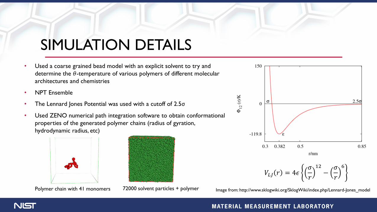
SIMULATION DETAILS• Used a coarse grained bead model with an explicit solvent to try and

determine the 𝜃-temperature of various polymers of different molecular

architectures and chemistries

• NPT Ensemble

• The Lennard Jones Potential was used with a cutoff of 2.5σ

• Used ZENO numerical path integration software to obtain conformational

properties of the generated polymer chains (radius of gyration,

hydrodynamic radius, etc)

𝑉𝐿𝐽 𝑟 = 4𝜖𝜎

𝑟

12

−𝜎

𝑟

6

Image from: http://www.sklogwiki.org/SklogWiki/index.php/Lennard-Jones_model72000 solvent particles + polymerPolymer chain with 41 monomers

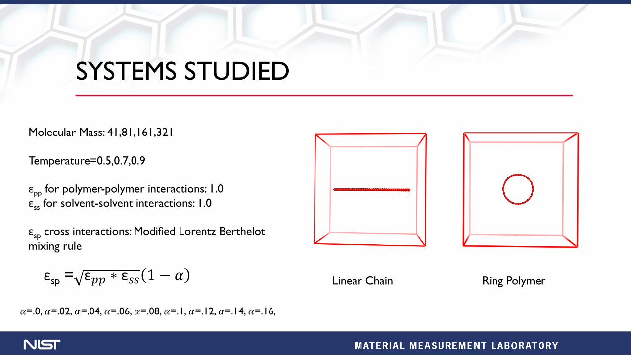
SYSTEMS STUDIED

Linear Chain Ring Polymer

Molecular Mass: 41,81,161,321

Temperature=0.5,0.7,0.9

εpp for polymer-polymer interactions: 1.0

εss for solvent-solvent interactions: 1.0

εsp cross interactions: Modified Lorentz Berthelot

mixing rule

εsp = ε𝑝𝑝 ∗ ε𝑠𝑠 1 − 𝛼

𝛼=.0, 𝛼=.02, 𝛼=.04, 𝛼=.06, 𝛼=.08, 𝛼=.1, 𝛼=.12, 𝛼=.14, 𝛼=.16,

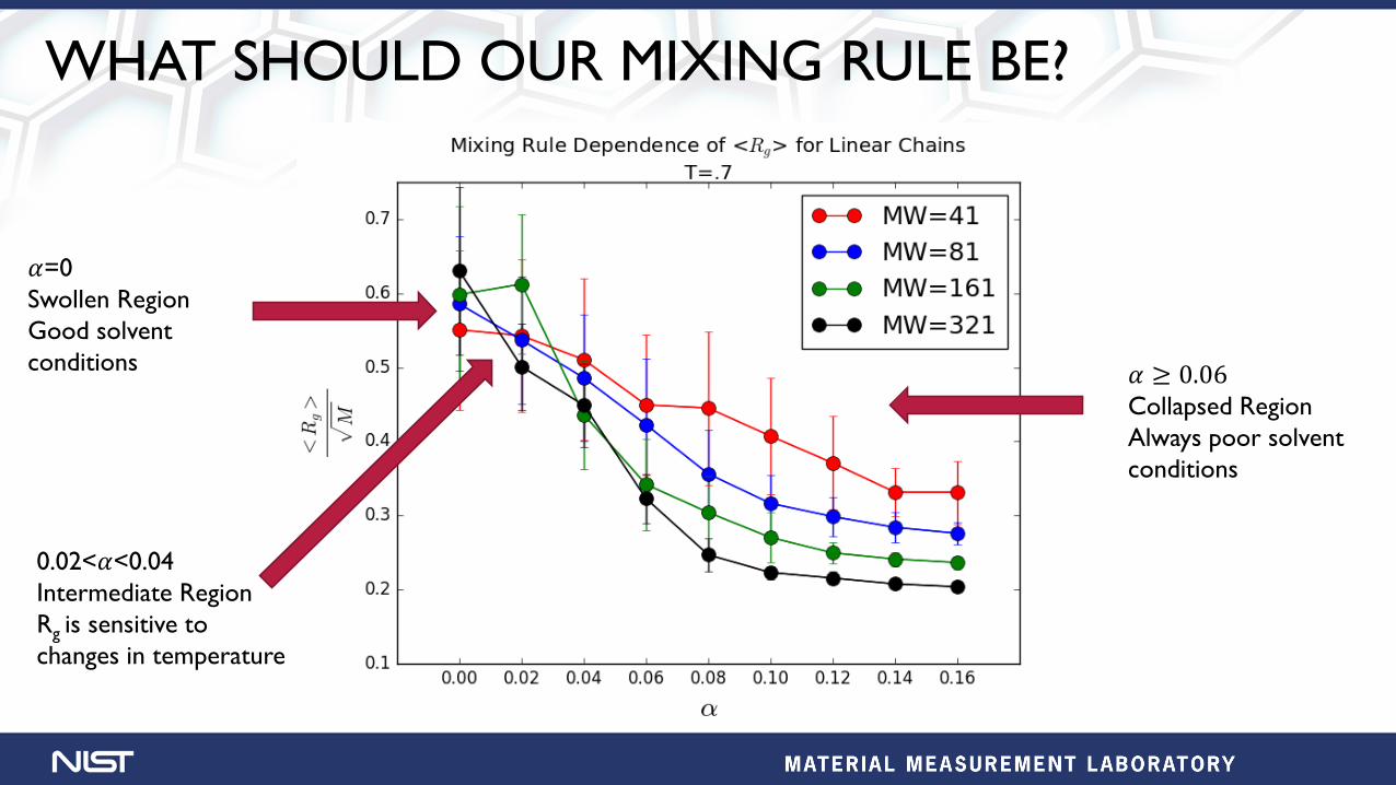
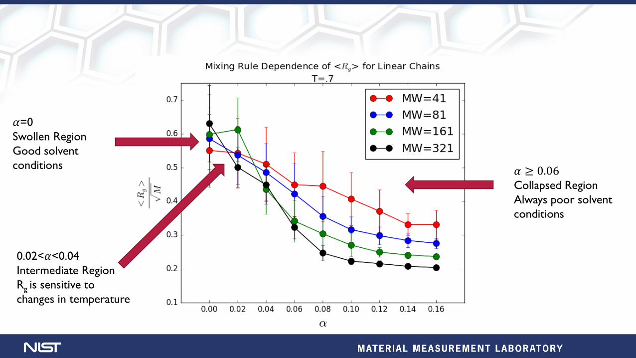
WHAT SHOULD OUR MIXING RULE BE?

𝛼 ≥ 0.06Collapsed Region

Always poor solvent

conditions

𝛼=0

Swollen Region

Good solvent

conditions

0.02<𝛼<0.04

Intermediate Region

Rg is sensitive to

changes in temperature

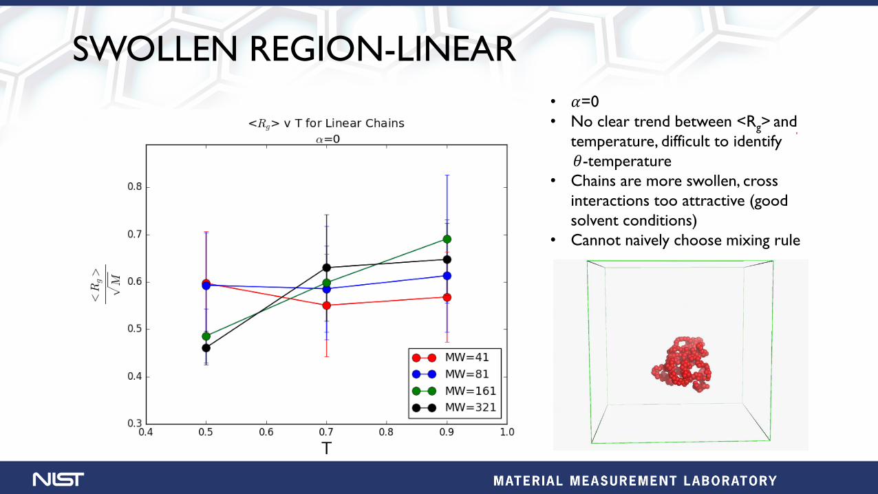
SWOLLEN REGION-LINEAR

• 𝛼=0

• No clear trend between <Rg> and

temperature, difficult to identify

𝜃-temperature

• Chains are more swollen, cross

interactions too attractive (good

solvent conditions)

• Cannot naively choose mixing rule

𝛼 ≥ 0.06Collapsed Region

Always poor solvent

conditions

𝛼=0

Swollen Region

Good solvent

conditions

0.02<𝛼<0.04

Intermediate Region

<Rg> is sensitive to

changes in temperature

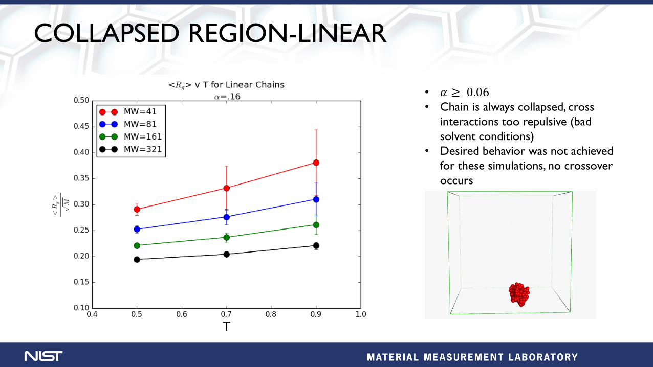
COLLAPSED REGION-LINEAR

• 𝛼 ≥ 0.06• Chain is always collapsed, cross

interactions too repulsive (bad

solvent conditions)

• Desired behavior was not achieved

for these simulations, no crossover

occurs

𝛼 ≥ 0.06Collapsed Region

Always poor solvent

conditions

𝛼=0

Swollen Region

Good solvent

conditions

0.02<𝛼<0.04

Intermediate Region

Rg is sensitive to

changes in temperature

INTERMEDIATE REGION-LINEAR

𝛼 = 0.02 𝛼 = 0.04

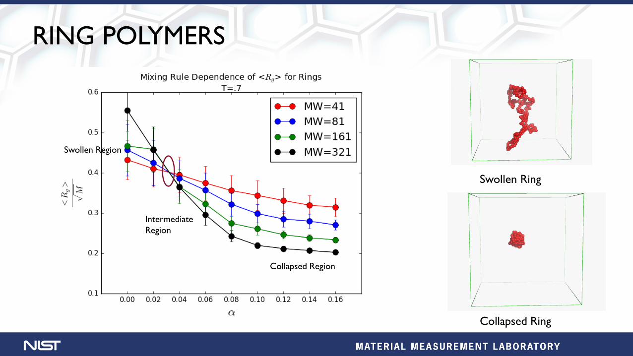
RING POLYMERS

Swollen Ring

Collapsed Ring

Collapsed Region

Intermediate

Region

Swollen Region

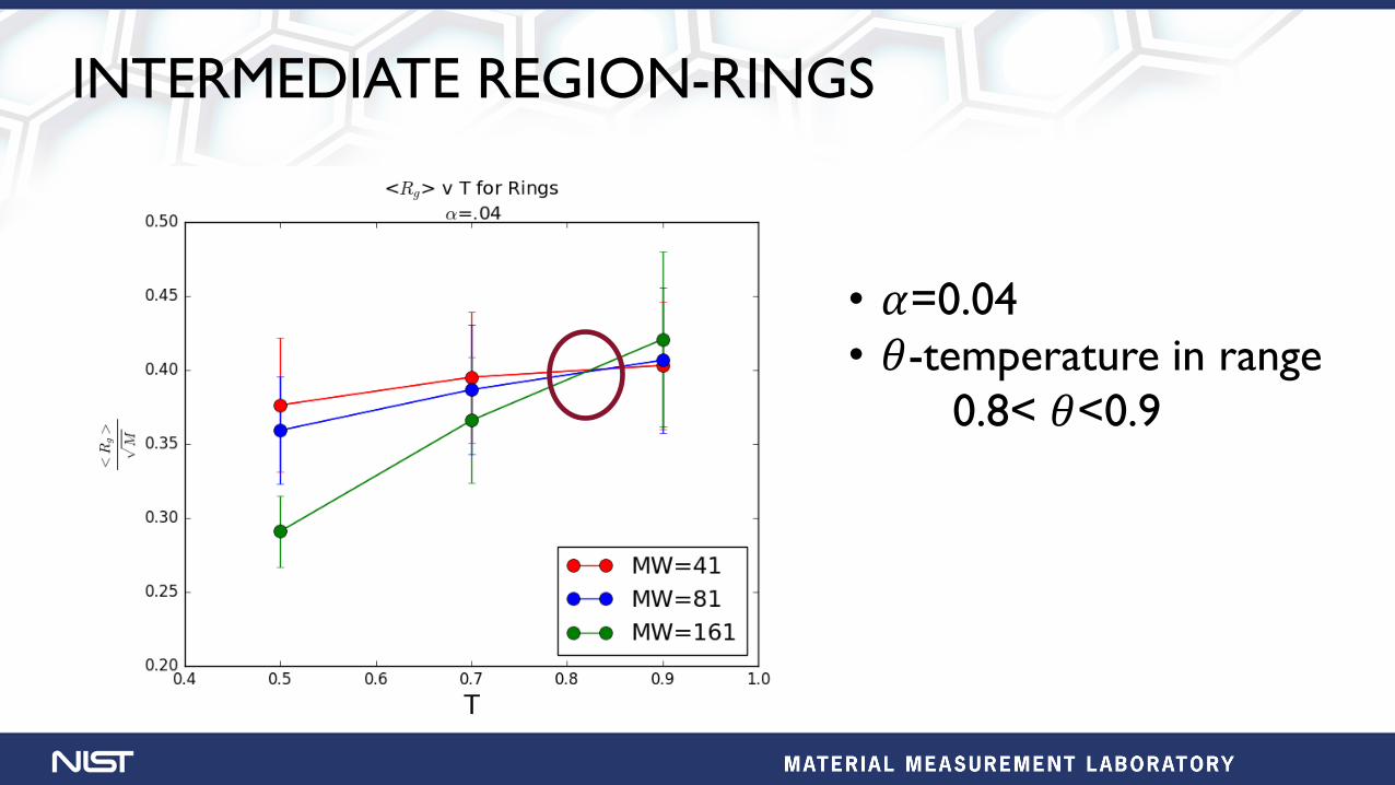
INTERMEDIATE REGION-RINGS

• 𝛼=0.04

• 𝜃-temperature in range

0.8< 𝜃<0.9

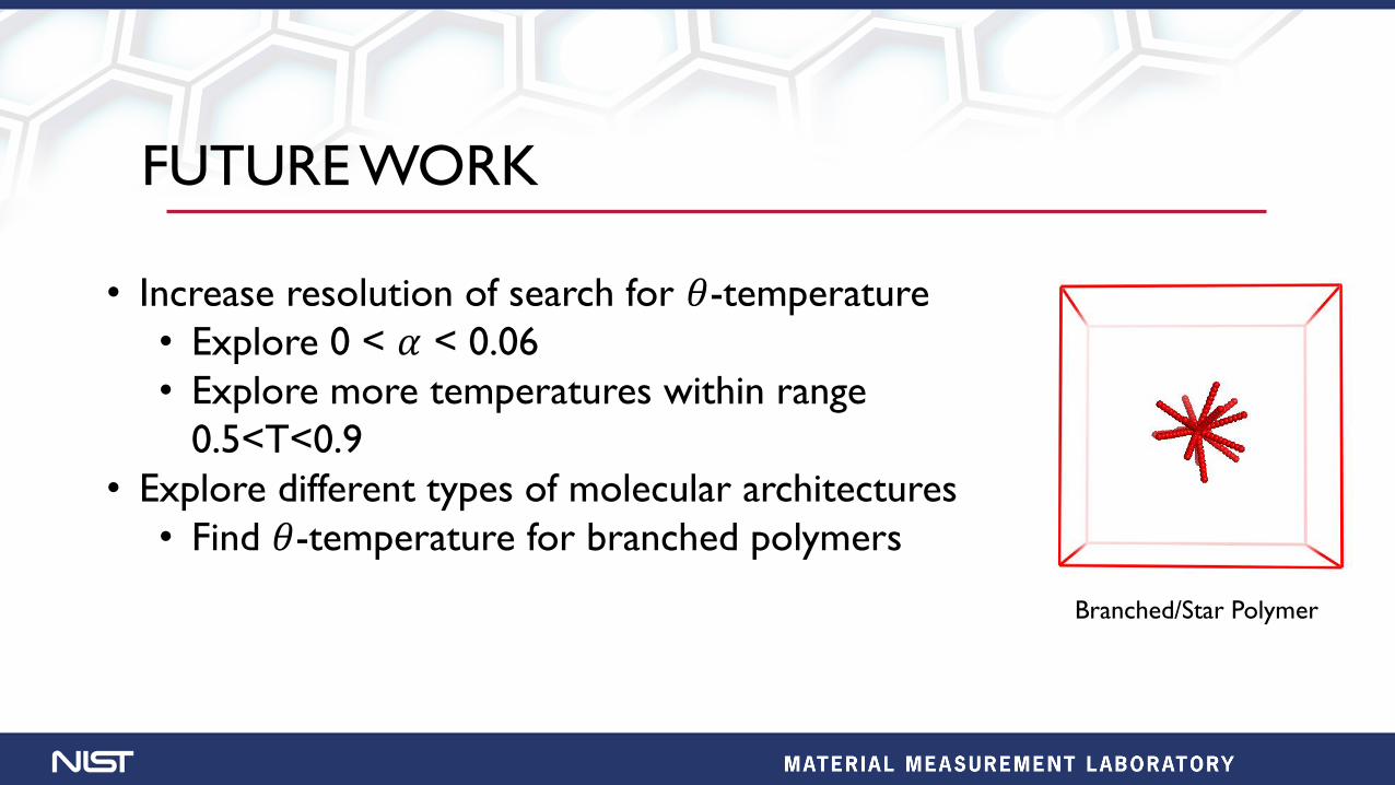
FUTURE WORK

• Increase resolution of search for 𝜃-temperature

• Explore 0 < 𝛼 < 0.06

• Explore more temperatures within range

0.5<T<0.9

• Explore different types of molecular architectures

• Find 𝜃-temperature for branched polymers

Branched/Star Polymer

ACKNOWLEDGMENTS

• Dr. Alexandros Chremos

• Dr. Jack Douglas

• Computational Soft Materials Working Group

(COMSOFT)

• NIST Material Measurement Laboratory (MML)

• NIST Summer Undergraduate Research Fellowship

(SURF) Program

• Le Moyne College