Infrared optical properties of α quartz by

molecular dynamics simulations

Fabrizio Gangemi∗ Roberto Gangemi∗ Andrea Carati†

Alberto Maiocchi† Luigi Galgani†

March 26, 2018

Abstract

This paper is concerned with theoretical estimates of the refractive–index curves for quartz, obtained by the Kubo formulæ in the classicalapproximation, through MD simulations for the motions of the ions. Twoobjectives are considered. The first one is to understand the role of non-linearities in situations where they are very large, as at the α–β structuralphase transition. We show that on the one hand they don’t play an essen-tial role in connection with the form of the spectra in the infrared. On theother hand they play an essential role in introducing a chaoticity whichinvolves a definite normal mode. This might explain why that mode isRaman active in the α phase, but not in the β phase. The second ob-jective concerns whether it is possible in a microscopic model to obtainnormal mode frequencies, or peak frequencies in the optical spectra, thatare in good agreement with the experimental data for quartz. Notwith-standing a lot of effort, we were unable to find results agreeing better thanabout 6%, as apparently also occurs in the whole available literature. Weinterpret this fact as indicating that some essential qualitative feature islacking in all models which consider, as the present one, only short–rangerepulsive potentials and unretarded long–range electric forces.

PACS: 78.20.Ci, 42.70.Ce, 63.20.Ry

1 Introduction

A subject of great current interest is that of a microscopic description of theferroelectric transition. It is known that at the transition a divergence of thedielectric constant ε(ω) at ω = 0 occurs, which in most cases is understood ascorresponding to the fact that the frequency of an infrared peak goes to zero. Onthe other hand, the infrared frequencies are usually studied via a linear analysis

∗DMMT, Universita di Brescia, Viale Europa 11, 25123 Brescia – Italy†Dep. Mathematics, Universita degli Studi di Milano, Via Saldini 50, 20133 Milano – Italy

1

arX

iv:1

609.

0195

7v1

[co

nd-m

at.m

trl-

sci]

7 S

ep 2

016

of phonon dispersion relations, while the nonlinear contribution to the dynamicsshould be relevant at the transition to the ferroelectric phase, as should be nearany phase transition. So the problem arises of how the infrared peaks shouldbe described in a fully nonlinear setting. A description can actually be giventhrough the study of the time autocorrelation of the polarization due to the ions,which can be computed in the classical approximation via molecular dynamicssimulations. Computations of this type were indeed performed successfully inthe case of LiF [1], with results that agree with the experimental data in asurprisingly good way.

At the moment, as will be explained below, we are unable to study ferro-electrics through molecular dynamics. So in this paper we limit ourselves toquartz, which is not a ferroelectric material, but however presents a divergencein the dielectric constant at the temperature of the α–β transition. We computehere its refractive index curves in the infrared region. Our main concerns arethe dynamical properties of the system, particularly at the α–β transition, andthe quantitative agreement between calculated and experimental spectra in theinfrared for α quartz.

As is well known [2], linear analysis shows that quartz is doubly refractiveand that the peaks in its refractive–index curves correspond to the frequencies ofthe active normal modes. Such qualitative results are confirmed by the presentmolecular dynamics simulations for α quartz at high temperatures, even at thetransition to the β phase, notwithstanding the high nonlinearity of the system.This quantitative agreement of the nonlinear results with those of the linearanalysis, in particular for the values of the frequencies, is quite surprising, inview of the large nonlinear contributions, and probably is due to some deepreason not yet fully understood. On the other hand, both the linear analysisand our nonlinear study fail in perfectly reproducing the experimental data,as some systematic deviations are observed. We tried several procedures forchoosing the parameters, both of the linear model and of the nonlinear one, inorder to find a better agreement with the experimental curves. But there wasno way of reducing the relative error below a threshold of the order of 6%. Thisfact, too, requires an explanation. These are the two main results of the presentwork.

2 The model

It is known that the primitive cell of quartz contains nine atoms (three siliconand six oxygen atoms). Moreover, it has the form of a right prism of rhomboidalbasis, corresponding to three basis vectors a,b, c with a and b forming an angleof 120◦ and c orthogonal to a and b. In Table 1 we report the lengths of thethree basis vectors at normal conditions of temperature and pressure (300 Kand 1 bar), as given by [3], which we use in our simulations. We also reportthe fractional coordinates x,y,z (along the three basis vectors) of a silicon atomand of an oxygen atom, out of which all other coordinates can be generated

2

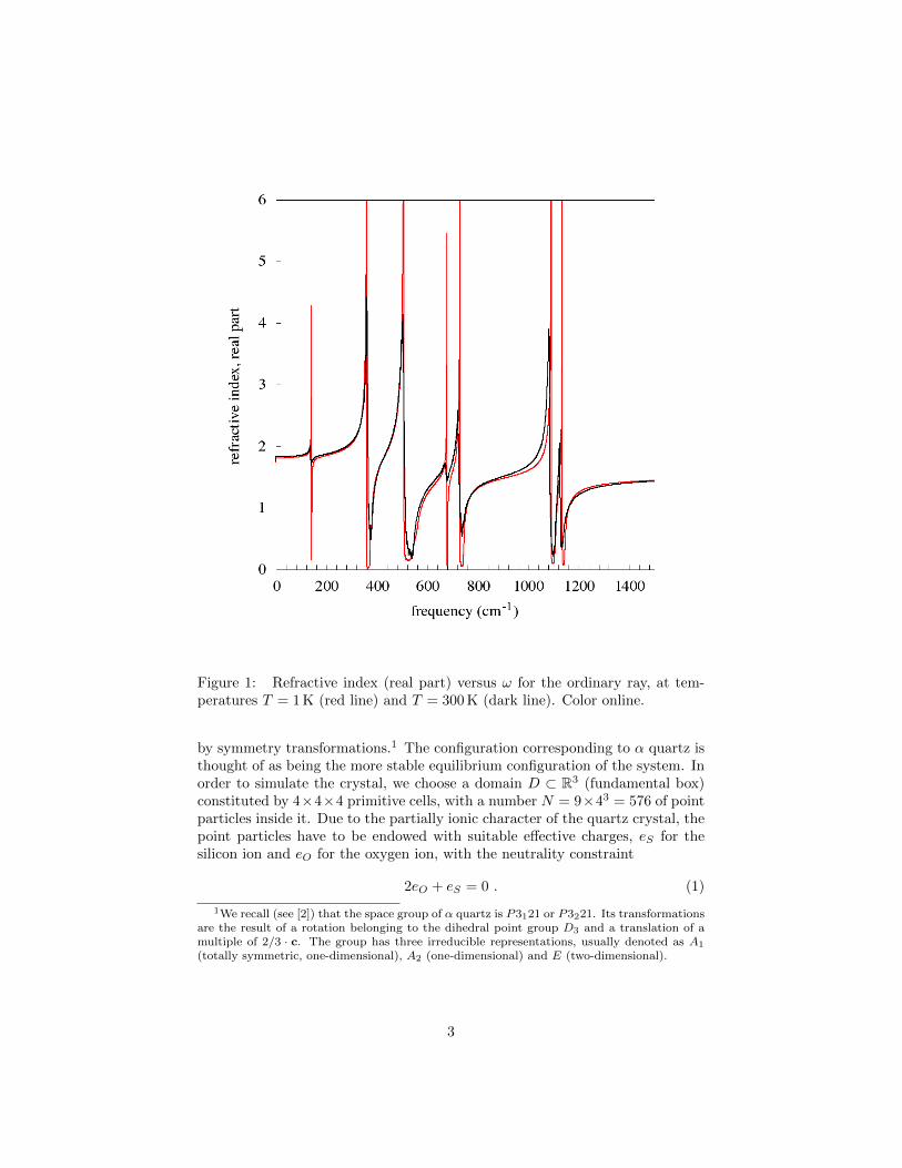
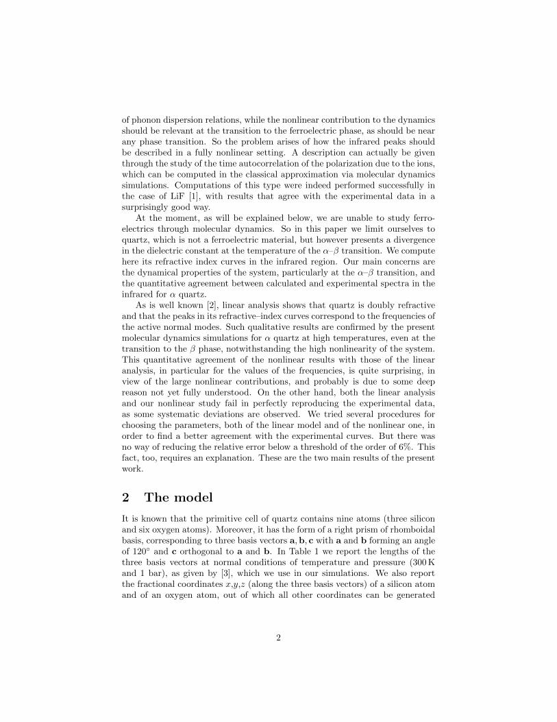
Figure 1: Refractive index (real part) versus ω for the ordinary ray, at tem-peratures T = 1 K (red line) and T = 300 K (dark line). Color online.

by symmetry transformations.1 The configuration corresponding to α quartz isthought of as being the more stable equilibrium configuration of the system. Inorder to simulate the crystal, we choose a domain D ⊂ R3 (fundamental box)constituted by 4×4×4 primitive cells, with a number N = 9×43 = 576 of pointparticles inside it. Due to the partially ionic character of the quartz crystal, thepoint particles have to be endowed with suitable effective charges, eS for thesilicon ion and eO for the oxygen ion, with the neutrality constraint

2eO + eS = 0 . (1)

1We recall (see [2]) that the space group of α quartz is P3121 or P3221. Its transformationsare the result of a rotation belonging to the dihedral point group D3 and a translation of amultiple of 2/3 · c. The group has three irreducible representations, usually denoted as A1

(totally symmetric, one-dimensional), A2 (one-dimensional) and E (two-dimensional).

3

Figure 2: Same as Figure 1 for the extraordinary ray.

Thus, Coulomb long range forces come into play and, in order to take them intoaccount, working however with a small numberN of particles, periodic boundaryconditions are imposed. In addition to the electric forces, short-range two-bodyspherically symmetric potentials are introduced, one for each of the pairs Si−Si,O−O, Si−O. These potentials are taken of a form which is extensively used forquartz, namely (see [4, 5]),

U(r) = Ae−Br − C

r6, (2)

(r being the interatomic distance), with a triple of parameters A, B, C a prioridifferent for each pair. In the numerical calculations, for the short-range inter-actions a cutoff of 9 A was imposed, while the Coulomb interactions were dealtwith through standard Ewald summations. This is exactly the point where somemodifications are required if one aims at dealing with ferroelectrics. Indeed theEwald resummation provides a periodic electric field having a vanishing mean,

4

at variance with what occurs with ferroelectrics. The problem of how to modifyaccordingly the Ewald procedure is left for a possible future work.

The masses are taken from the literature, so that to fix the model thereremains a total of 10 free parameters: one effective charge (for example that ofoxygen) and the three parameters A, B, C of the short-range potential for eachof the three pairs Si−O, O−O, Si−Si. The values of the potential parametersadopted are reported in Table 2, while we used the values eS = 2.04191 andeO = −1.02096 for the effective charge (in unit of electron charge) of Si andO respectively. They were determined by optimization procedures aimed atobtaining the best possible agreement between the computed refractive indexcurves and the empirical ones at 300 K, requiring in addition that the α structurebe stable at that temperature and at larger (but not too much) temperatures.With the values thus determined for the parameters of the model it turns out, aswill be shown below, that the α–β transition occurs at a temperature of aboutT = 700 K, which is a rather low value. We leave for a future work the taskof performing an optimization of the parameters with a procedure which takesboth the frequencies and the transition temperature into account.

The equations of motion were numerically solved using a Verlet algorithm,with integration step of 2 fs, at several values of temperature. Having chosento work in a purely Hamiltonian frame, temperature was determined throughthe choice of the initial data. In principle this should be obtained by extract-ing the data according to a Gibbs distribution. This being impracticable, wefollowed the alternative standard procedure. Namely, one puts the particles atthe α equilibrium point, while their velocities are extracted from a Maxwell–Boltzmann distribution at a suitable temperature. Then one lets the systemthermalize, which usually takes a time of the order of 2 ps (1000 integrationsteps), and temperature is eventually identified through the mean kinetic en-ergy of the ions. Then one starts computing means and correlations of therelevant quantities.

α quartz parametersa b c

4.9137 A 4.9137 A 5.4047 Ax y z

Si 0.4697 0.0000 0.0000O 0.4133 0.2672 0.1188

β quartz parametersa b c

4.9965 A 4.9965 A 5.4546 Ax y z

Si 0.5000 0.0000 0.0000O 0.4157 0.2078 0.1667

Table 1: Geometric parameters for α and β quartz (see text).

5

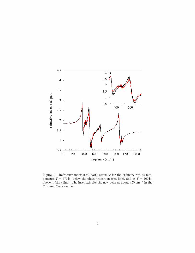
Figure 3: Refractive index (real part) versus ω for the ordinary ray, at tem-perature T = 670 K, below the phase transition (red line), and at T = 700 K,above it (dark line). The inset exhibits the new peak at about 455 cm−1 in theβ phase. Color online.

6

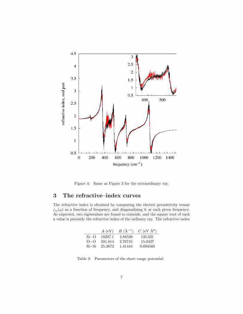
Figure 4: Same as Figure 3 for the extraordinary ray.

3 The refractive–index curves

The refractive index is obtained by computing the electric permittivity tensorεij(ω) as a function of frequency, and diagonalizing it at each given frequency.As expected, two eigenvalues are found to coincide, and the square root of sucha value is precisely the refractive index of the ordinary ray. The refractive index

A (eV) B (A−1) C (eV A6)

Si−O 18207.1 4.88538 135.021O−O 501.814 2.76745 15.0427Si−Si 25.3672 1.41444 0.694560

Table 2: Parameters of the short range potential.

7

of the extraordinary ray is instead the square root of the remaining eigenvalue.2

The connection with dynamics is obtained through the susceptibility tensorχij(ω) due to the ions, which is related to permittivity by

εij(ω) = δij + 4π(χij(ω) + χelij

). (3)

Here, χel is the contribution of the electrons, which turns out to be constant inthe infrared domain (see [6]). Instead, the ions’ contribution χij(ω) is obtainednumerically according to Green-Kubo linear response theory (see for example[7]) as follows. One considers the polarization P, which is defined in microscopicterms as

P =1

V

∑l

elxl , (4)

where V is the volume of the simulation domain (or fundamental box), while xlis the position vector of the l–th ion, of charge el.

Then at temperature T one has

χij(ω) =V

kBT

∫ +∞

0

e−iωt〈Pi(t)Pj(0)〉dt , (5)

kB being the Boltzmann constant. Here 〈·〉 should in principle be the canonicalaverage. Actually the averages were estimated as the mean of the time averagescalculated along a certain number (usually 40) of different MD trajectories,calculated for 200 ps.

A first set of results is illustrated in Figures 1 and 2. In the first figure wereport, vs frequency, the real part of the refractive index for the ordinary ray atT = 300 K (dark line) and at T = 1 K (red line). The analogous spectra for theextraordinary ray are reported in Figure 2. At a temperature as low as T = 1 Kthe spectrum is determined essentially by the linear approximation, so that thepeaks correspond to the frequencies of the normal modes (actually, those ofthe so called type A2 and E; see [2]). The results show that the spectrum atT = 300 K does not differ essentially from that corresponding to 1 K, apart froma consistent broadening of the peaks and some small shifts in their frequencies.

A second set of results concerns the behavior of the spectra at the structuralα–β phase transition which, in the present microscopic model, with the choicemade for the parameters, turns out to occur in a region of temperatures roughlyaround T = 690 K. This will be shown in a moment. So we computed therefractive–index curves at T = 670 K, an T = 700 K, which are reported inFigure 3 for the ordinary ray and in Figure 4 for the extraordinary ray.

The figures show that, at the transition, the optical spectra are still dom-inated by the linear behavior. Indeed, in both figures the two curves relativeto the two temperatures essentially superpose one another, and one can noticethe same peaks of the previous Figures 1 e 2, just a little more broadened andnoisy.

2It may be useful to keep to the following criterion: the eigenvalue corresponding to theeigenvector with larger component along the c-axis of the lattice is always associated with theextraordinary ray.

8

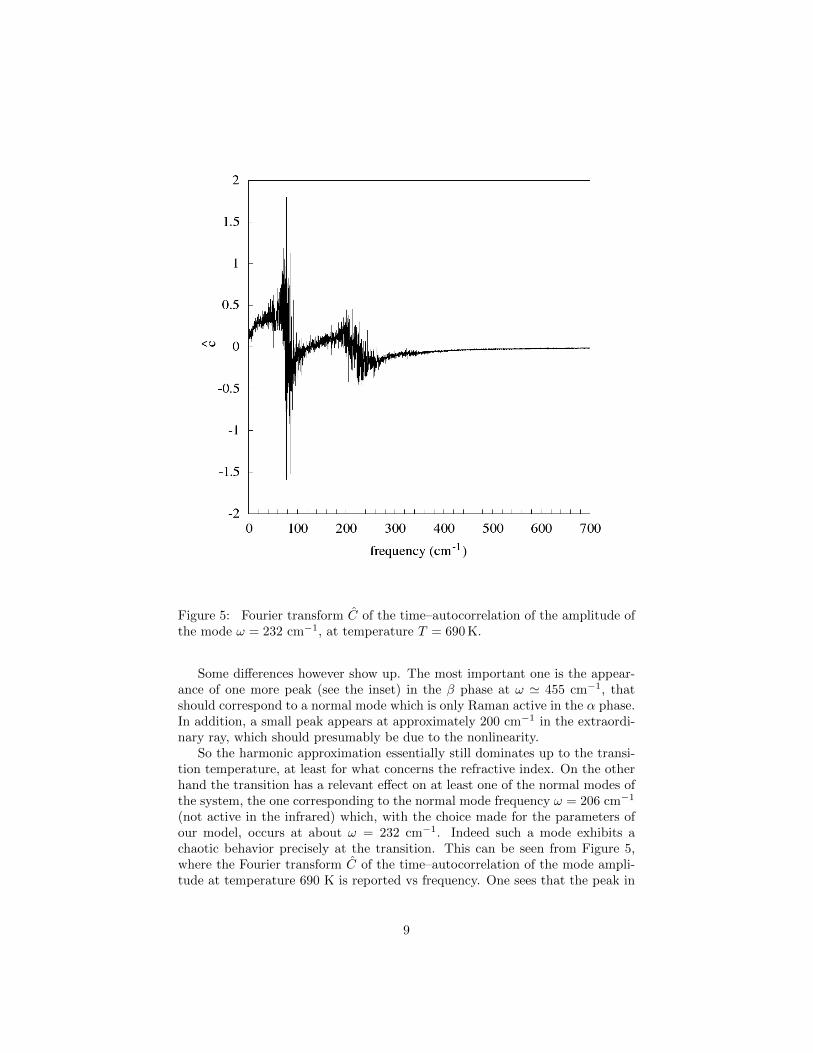
Figure 5: Fourier transform C of the time–autocorrelation of the amplitude ofthe mode ω = 232 cm−1, at temperature T = 690 K.

Some differences however show up. The most important one is the appear-ance of one more peak (see the inset) in the β phase at ω ' 455 cm−1, thatshould correspond to a normal mode which is only Raman active in the α phase.In addition, a small peak appears at approximately 200 cm−1 in the extraordi-nary ray, which should presumably be due to the nonlinearity.

So the harmonic approximation essentially still dominates up to the transi-tion temperature, at least for what concerns the refractive index. On the otherhand the transition has a relevant effect on at least one of the normal modes ofthe system, the one corresponding to the normal mode frequency ω = 206 cm−1

(not active in the infrared) which, with the choice made for the parameters ofour model, occurs at about ω = 232 cm−1. Indeed such a mode exhibits achaotic behavior precisely at the transition. This can be seen from Figure 5,where the Fourier transform C of the time–autocorrelation of the mode ampli-tude at temperature 690 K is reported vs frequency. One sees that the peak in

9

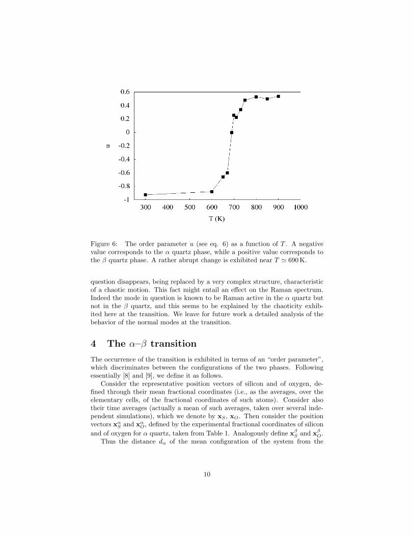
Figure 6: The order parameter u (see eq. 6) as a function of T . A negativevalue corresponds to the α quartz phase, while a positive value corresponds tothe β quartz phase. A rather abrupt change is exhibited near T ' 690 K.

question disappears, being replaced by a very complex structure, characteristicof a chaotic motion. This fact might entail an effect on the Raman spectrum.Indeed the mode in question is known to be Raman active in the α quartz butnot in the β quartz, and this seems to be explained by the chaoticity exhib-ited here at the transition. We leave for future work a detailed analysis of thebehavior of the normal modes at the transition.

4 The α–β transition

The occurrence of the transition is exhibited in terms of an “order parameter”,which discriminates between the configurations of the two phases. Followingessentially [8] and [9], we define it as follows.

Consider the representative position vectors of silicon and of oxygen, de-fined through their mean fractional coordinates (i.e., as the averages, over theelementary cells, of the fractional coordinates of such atoms). Consider alsotheir time averages (actually a mean of such averages, taken over several inde-pendent simulations), which we denote by xS , xO. Then consider the positionvectors xαS and xαO, defined by the experimental fractional coordinates of silicon

and of oxygen for α quartz, taken from Table 1. Analogously define xβS and xβO.Thus the distance dα of the mean configuration of the system from the

10

equilibrium α configuration is naturally estimated as

dα =√‖xS − xαS‖2 + ‖xO − xαO‖2 ,

and analogously for the distance dβ from the equilibrium β configuration. Soone can introduce the variable u defined by

u =dα − dβdα,β

(6)

where dα,β is a normalizing factor, the distance between the two equilibria,defined in the natural way.

A negative value of u clearly indicates that the atoms are, in the mean,near to the α configuration, while a positive value indicates that they are in themean near to the β configuration. The graph of u vs temperature, is reportedin Figure 6. One sees that a rather abrupt passage from a negative to a positivevalue occurs in a small region of temperatures about T = 690 K, at which a valueof u very near to zero is obtained. Instead a value of about −0.6 is obtainedat T = 670 K and a value of about +0.25 is obtained at T = 700 K. Thisshows that at these temperatures the nonlinear effects become so important asto trigger a phase transition.

5 Comparison with the experimental data

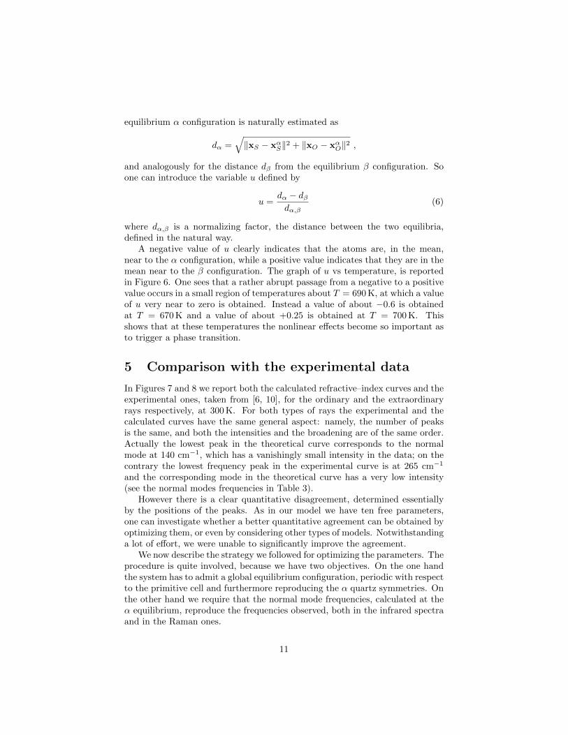
In Figures 7 and 8 we report both the calculated refractive–index curves and theexperimental ones, taken from [6, 10], for the ordinary and the extraordinaryrays respectively, at 300 K. For both types of rays the experimental and thecalculated curves have the same general aspect: namely, the number of peaksis the same, and both the intensities and the broadening are of the same order.Actually the lowest peak in the theoretical curve corresponds to the normalmode at 140 cm−1, which has a vanishingly small intensity in the data; on thecontrary the lowest frequency peak in the experimental curve is at 265 cm−1

and the corresponding mode in the theoretical curve has a very low intensity(see the normal modes frequencies in Table 3).

However there is a clear quantitative disagreement, determined essentiallyby the positions of the peaks. As in our model we have ten free parameters,one can investigate whether a better quantitative agreement can be obtained byoptimizing them, or even by considering other types of models. Notwithstandinga lot of effort, we were unable to significantly improve the agreement.

We now describe the strategy we followed for optimizing the parameters. Theprocedure is quite involved, because we have two objectives. On the one handthe system has to admit a global equilibrium configuration, periodic with respectto the primitive cell and furthermore reproducing the α quartz symmetries. Onthe other hand we require that the normal mode frequencies, calculated at theα equilibrium, reproduce the frequencies observed, both in the infrared spectraand in the Raman ones.

11

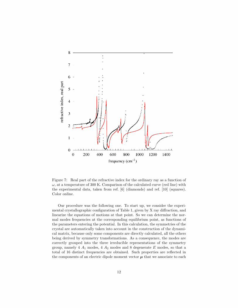
Figure 7: Real part of the refractive index for the ordinary ray as a function ofω, at a temperature of 300 K. Comparison of the calculated curve (red line) withthe experimental data, taken from ref. [6] (diamonds) and ref. [10] (squares).Color online.

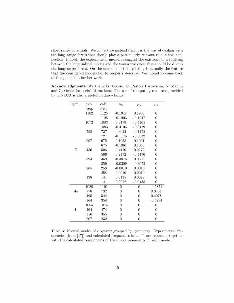
Our procedure was the following one. To start up, we consider the experi-mental crystallographic configuration of Table 1, given by X ray diffraction, andlinearize the equations of motions at that point. So we can determine the nor-mal modes frequencies at the corresponding equilibrium point, as functions ofthe parameters entering the potential. In this calculation, the symmetries of thecrystal are automatically taken into account in the construction of the dynami-cal matrix, because only some components are directly calculated, all the othersbeing derived by symmetry transformations. As a consequence, the modes arecorrectly grouped into the three irreducible representations of the symmetrygroup, namely 4 A1 modes, 4 A2 modes and 8 degenerate E modes, so that atotal of 16 distinct frequencies are obtained. Such properties are reflected inthe components of an electric dipole moment vector µ that we associate to each

12

Figure 8: Same as Figure 7 for the extraordinary ray. Here, however, theexperimental data (diamonds) are taken only from ref. [6].

mode by multiplying the Cartesian displacement of each atom by its effectivecharge and summing all the vectors thus obtained (see Table 3). This gives aneasy criterion for the correct identification of frequencies in the minimizationprocedure, i.e. in the search for the parameters of the potential that minimizethe function

W =1

16

16∑i

(ωi − ωexiωexi

)2

, (7)

where ωexi are the experimental values. This optimization procedure was per-formed using a simulated annealing algorythm [11], especially useful for multi-variate functions. Actually this algorithm provides many different solutions tothe optimization problem, possibly due to the presence of many local minimain the function that has to be minimized.

Then, for any single set of parameters obtained we determine the correspond-ing equilibrium position and the corresponding set of normal mode frequencies.

13

The set of parameters is accepted if the calculated equilibrium position is suffi-ciently near to the experimental one of α quartz, the frequencies are sufficientlynear to the experimental ones, and furthermore the α structure is stable up tosufficiently high temperatures. No set of parameters found gave an agreementfor the frequencies better than about 6–7%.

Other attempts were as follows. We started from the power n = 6 entering(2), letting n be a free parameter, different for each pair, adapting the cutoffparameter to each choice. No substantial improvement was obtained. Then wechanged completely the form of the potentials, using Lennard–Jones ones. Butthis gave a drastic worsening of the results.

These facts show that the results depend in a very sensitive way on theform of the potentials. In order to bypass this problem we decided to restrictour studies to the linear model, assigning as parameters directly the elasticconstants. In such a way one even eliminates the constraint that the elasticconstants should be defined in terms of first and second derivatives of a givenpotential. However, no progress was obtained.

As a last resort, we eliminated the neutrality constraint (1) on the effectivecharge, by assuming both charges to be free parameters, but again withoutsubstantial improvement.

Actually, in the whole literature we were unable to find a paper in whichthe calculated frequencies agree with the experimental ones, in the mean, betterthan 3%, which is the result obtained in the old paper [12]. In such a papera linear model is considered, which takes into account also the polarization ofoxygen ions as a free parameter. However, the maximum error was larger than7%.

In the more recent paper [13], a nonlinear model was investigated by MDsimulations. Both the short range potentials and the ions polarizability wereobtained through ab initio computations, but again, in the very words of theauthors, “The calculated frequencies are systematically underestimated, but dif-ferences are below 7%–8%.”. The authors point out that their results constitutean improvement with respect to those of previous works, for example those ofpaper [14], in which “The discrepancy in the lower energy bending vibrationsis somewhat higher, usually around 10–20%”. The authors of [13] ascribe theimprovement to the fact of having taken the ions’ polarization into account.

Neither does the consideration of three–body potentials, apparently, improvethe agreement between computed and observed frequencies. For example, inpaper [9] the errors can reach 20% for some modes (see their Table V), as alsooccurs in paper [15] where for example (see fig. 10) one of the computed lineslies near 600 cm−1, against the observed value near to 500 cm−1.

We interpret these facts as indicating that some structural deficiency ispresent in all models (including ours) that have been considered. Such a de-ficiency was sometimes acknowledged. For example, in paper [16] it is statedthat “The deviations of the calculation with respect to the experiment are notrandom, but systematic: the higher phonon frequencies, above the mean, are in-variably too low with respect to the experiment, while the lower frequencies areinvariably too high.”. These facts are usually ascribed to some deficiency in the

14

short range potentials. We conjecture instead that it is the way of dealing withthe long–range forces that should play a particularly relevant role in this con-nection. Indeed, the experimental measures suggest the existence of a splittingbetween the longitudinal modes and the transverse ones, that should be due tothe long–range forces. On the other hand this splitting is actually the featurethat the considered models fail to properly describe. We intend to come backto this point in a further work.

Acknowledgments. We thank G. Grosso, G. Pastori Parravicini, N. Maniniand G. Onida for useful discussions. The use of computing resources providedby CINECA is also gratefully acknowledged.

sym. exp. calc. µx µy µzfreq. freq.1162 1125 -0.1947 0.1903 0

1125 -0.1903 -0.1947 01072 1083 0.3479 -0.4105 0

1083 -0.4105 -0.3479 0795 727 0.3032 -0.1175 0

727 -0.1175 -0.3032 0697 675 0.1058 0.1061 0

675 -0.1061 0.1058 0E 450 506 0.4470 0.2172 0

506 0.2172 -0.4470 0394 359 -0.3075 0.0309 0

359 -0.0309 -0.3075 0265 258 -0.0010 0.0010 0

258 0.0010 0.0010 0128 141 0.0435 0.0072 0

141 0.0072 -0.0435 01080 1101 0 0 -0.5871

A2 778 732 0 0 0.3754495 544 0 0 0.4078364 358 0 0 -0.42941085 1074 0 0 0

A1 464 474 0 0 0356 355 0 0 0207 232 0 0 0

Table 3: Normal modes of α quartz grouped by symmetry. Experimental fre-quencies (from [17]) and calculated frequencies in cm−1 are reported, togetherwith the calculated components of the dipole moment µ for each mode.

15

References

[1] Gangemi F., Carati A., Galgani L., Gangemi R., Maiocchi A.,Europhys. Lett 110, (2015) 47003.

[2] Spitzer W.G., Kleinman D.A., Phys. Rev. 121, (1961) 1324.

[3] Kihara K., Eur. J. Mineral. 2, (1990) 63.

[4] Tsuneyuki S., Tsukada M., Aoki H., Matsui Y., Phys. Rev. Lett. 61,(1988) 869.

[5] Kramer G. J., Farragher N. P., van Beest B. W. H., van SantenR. A., Phys. Rev. B 43, (1991) 5068.

[6] Palik E., Handbook of optical constants of solids (Academic Press, Ams-terdam) (1998), p. 719.

[7] Carati A., Galgani L., Eur. Phys. J. D 68, (2014) 307.

[8] Tsuneyuki F., Aoki H., Tsukada M., Matsui Y., Phys. Rev. Lett 64,(1990) 776.

[9] Ma W., Garofalini S.H., Phys. Rev. B 73, (2006) 174109.

[10] Cummings K. D., Tanner D. B., J. Opt. Soc. Am. 70, (1980) 123.

[11] Kirkpatrick S., Gelatt Jr. C. D., Vecchi M. P., Science 220,(1983) 671

[12] Iishi K., Zeits. f. Kristall. 144, (1976) 289.

[13] Liang Y., Miranda C.R., Scandolo S., J. Chem. Phys 125, (2006)194524.

[14] Tse S., Klug D.D., J. Chem. Phys. 95, (1991) 9176.

[15] Huang L., Kieffer J., J. Chem Phys. 118, (2003) 1487.

[16] Della Valle R.G., Andersen H.G., J. Chem. Phys. 94, (1991) 5056.

[17] Scott J.F., Porto S.P.S., Phys. Rev. 161, (1967) 903.

16