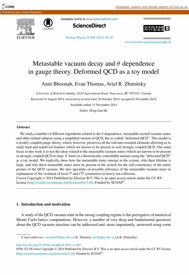
Available online at www.sciencedirect.com

CORE Metadata, citation and similar papers at core.ac.uk

Provided by Open Access Repository

ScienceDirect

Nuclear Physics B 890 (2015) 30–47

www.elsevier.com/locate/nuclphysb

Metastable vacuum decay and θ dependencein gauge theory. Deformed QCD as a toy model

Amit Bhoonah, Evan Thomas, Ariel R. Zhitnitsky

University of British Columbia, 6224 Agricultural Road, Vancouver, BC V6T1Z1, Canada

Received 14 August 2014; received in revised form 29 October 2014; accepted 6 November 2014

Available online 11 November 2014

Editor: Hong-Jian He

Abstract

We study a number of different ingredients related to the θ dependence, metastable excited vacuum states and other related subjects using a simplified version of QCD, the so-called “deformed QCD”. This model is a weakly coupled gauge theory, which, however, preserves all the relevant essential elements allowing us to study hard and nontrivial features which are known to be present in real strongly coupled QCD. Our main focus in this work is to test the ideas related to the metastable vacuum states (which are known to be present in strongly coupled QCD in large N limit) in a theoretically controllable manner using the “deformed QCD” as a toy model. We explicitly show how the metastable states emerge in the system, why their lifetime is large, and why these metastable states must be present in the system for the self-consistency of the entire picture of the QCD vacuum. We also speculate on possible relevance of the metastable vacuum states in explanation of the violation of local P and CP symmetries in heavy ion collisions.Crown Copyright © 2014 Published by Elsevier B.V. This is an open access article under the CC BY license (http://creativecommons.org/licenses/by/3.0/). Funded by SCOAP3.

1. Introduction and motivation

A study of the QCD vacuum state in the strong coupling regime is the prerogative of numerical Monte Carlo lattice computations. However, a number of very deep and fundamental questions about the QCD vacuum structure can be addressed and, more importantly, answered using some

E-mail addresses: zucchini@phas.ubc.ca (E. Thomas), arz@phas.ubc.ca (A.R. Zhitnitsky).

http://dx.doi.org/10.1016/j.nuclphysb.2014.11.0070550-3213/Crown Copyright © 2014 Published by Elsevier B.V. This is an open access article under the CC BY license (http://creativecommons.org/licenses/by/3.0/). Funded by SCOAP3.

A. Bhoonah et al. / Nuclear Physics B 890 (2015) 30–47 31

simplified versions of QCD. In the present paper, we study a set of questions related to metastable vacuum states and their decay to the true vacuum state using the so-called “deformed QCD” toy model wherein we can work analytically. This model describes a weakly coupled gauge theory, which, however, preserves many essential elements expected for true QCD, such as confinement, degenerate topological sectors, proper θ dependence, etc. This allows us to study difficult and nontrivial features, particularly related to vacuum structure, in an analytically tractable manner.

The fact that some high energy metastable vacuum states must be present in a gauge theory system in the large N limit has been known for quite some time [1]. A similar conclusion also follows from the holographic description of QCD as originally discussed in [2]. Furthermore, it has been known since [3] that the decay rate of these excited vacua in large N limit in strongly coupled pure gauge theory can be estimated as Γ ∼ exp(−N4).

The fundamental observation on the emergence of these excited vacuum states was made in a course of studies related to the resolution of the U(1)A problem in QCD in the large Nlimit [4–6]. In the present work we do not introduce quarks (which play an essential role in the formulation of the U(1)A problem) into the system, but, rather, study pure gluodynamics, and the metastable vacuum states which occur there. Nevertheless, the key object relevant for the resolution of the U(1)A problem, the so-called topological susceptibility χ , still emerges in our discussions in pure gluodynamics because it plays an important role in understanding of the spectrum of the ground state and multiple metastable states. Indeed, the topological suscepti-

bility is defined as χ(θ) = ∂2Evac(θ)

∂θ2 . Therefore, the information about the ground (or in general metastable) states Evac(θ) is related to the θ behaviour of the system formulated in terms of the topological susceptibility χ(θ).

When some deep questions are studied in a simplified version of a theory, there is always a risk that some effects which emerge in the simplified version of the theory could be just artifacts of the approximation, rather than genuine consequences of the original underlying theory. Our study using the “deformed QCD” as a toy model is not free from this potential difficulty with misinterpretation of artifacts as inherent features underlying QCD. Nevertheless, there are few strong arguments suggesting that we indeed study some intrinsic features of the system rather than some artificial effects. The first argument is discussed in the original paper on “deformed QCD” [7] where it has been claimed that this model describes a smooth interpolation between strongly coupled QCD and the weakly coupled “deformed QCD” without any phase transition. In addition, there are a few more arguments based on our previous experience with the “deformed QCD” model, see below, which also strongly suggest that we indeed study some intrinsic features of QCD rather than some artifact of the deformation.

Our arguments are based on the computation [8] of the contact term in the “deformed QCD”, see also [9] with some related discussions. The key point is that this contact term with a pos-itive sign (in the Euclidean formulation) in the topological susceptibility χ is required for the resolution of the U(1)A problem [4–6]. At the same time, any physical propagating degrees of freedom must contribute with a negative sign, see [8] with details. In [4] this positive contact term has been simply postulated while in [5,6] an unphysical Veneziano ghost was introduced into the system to saturate this term with the “wrong” sign in the topological susceptibility. This entire, very non-trivial picture, has been successfully confirmed by numerical lattice computa-tions. More importantly for the present studies, this picture has been supported by analytical computations in “deformed QCD” in which all the nontrivial crucial elements for the resolution of the U(1)A problem indeed emerge in analytical analysis.

Indeed, the non-dispersive contact term in topological susceptibility can be explicitly com-puted in this model and is given by [8]

32 A. Bhoonah et al. / Nuclear Physics B 890 (2015) 30–47

χcontact =ˆ

d4x⟨q(x), q(0)

⟩ ∼ˆ

d3x[δ(x)

], (1)

where q(x) is the topological density operator. It has the required “wrong sign” as this contri-bution is not related to any physical propagating degrees of freedom, but is rather related to the topological structure of the theory, and has a δ(x) function structure as it should. In this model χ is saturated by fractionally charged weakly interacting monopoles describing the tunnelling transitions between topologically distinct, but physically equivalent topological winding sectors. Furthermore, the δ(x) function in (1) should be understood as total divergence related to the infrared (IR) physics, rather than to ultraviolet (UV) behaviour as explained in [8]

χcontact ∼ˆ

δ(x) d3x =ˆ

d3x∂μ

(xμ

4πx3

). (2)

The singular behaviour of the contact term has been confirmed by the lattice computations where it has been found that the singular behaviour at x → 0 is an inherent IR feature of the underlying QCD rather than some lattice size effect [10–13].

In addition, one can explicitly see how the Veneziano ghost postulated in [5,6] is explicitly expressed in terms of auxiliary topological fields which saturate the contact term (1) in this model [14]. In other words, the η′ field in this model generates its mass (which is precisely the formulation of the U(1)A problem) as a result of a mixture of the Goldstone field with the topological auxiliary field governed by a Chern–Simons like action, see [14] for the details.

All these features related to the θ dependence which are known to be present in strongly coupled regime also emerge in the weakly coupled “deformed QCD” toy model. Therefore, we interpret such behaviour as a strong argument supporting our assumption that the “deformed QCD” model properly describes, at least qualitatively, the features related to the θ dependence and vacuum structure of QCD, including the presence of metastable states which is main subject of the present work.

The specific computations we perform related to the metastable vacuum states have never been performed using numerical lattice (or any other) methods. Therefore, we do not have the same level of luxury present in our previous studies of the contact term [8] in which our results were supported by numerous lattice computations. Nevertheless, as the specific questions about the metastable states are closely related to much more generic studies of the θ dependence in the system, as reviewed above, we are still confident that our results presented below, based on the “deformed QCD” model, are inherent qualitative properties of QCD rather than some artificial effects which may occur due to the deformation.

Our presentation is organized as follows. We start in Section 2 by reviewing a simplified (“deformed”) version of QCD which, on one hand, is a weakly coupled gauge theory wherein computations can be performed in theoretically controllable manner. On other hand, this de-formation preserves all the elements relevant to our study such as confinement, degeneracy of topological sectors, nontrivial θ dependence, presence of non-dispersive contribution to topo-logical susceptibility, and other crucial aspects pertinent to the study of the metastable states. In Section 2.2 we explicitly demonstrate the presence of metastable states in this model. In Sec-tion 3 we review the general strategy to compute a decay of metastable vacuum states to the true vacuum in the path integral formulation. Finally, in Section 4 we present our numerical analysis on the lifetime of the metastable states as a function of a “semi-classicality” which is a parameter determining the region of validity of our semiclassical computations. We conclude in Section 5 with speculations on possible consequences and manifestations of our results for physics of heavy ion collisions where a metastable state might be formed as a result of collision,

A. Bhoonah et al. / Nuclear Physics B 890 (2015) 30–47 33

and the system, which is order the size of a nuclei, might be locked in this state for sufficiently long period of time ∼10 fm/c.

2. Deformed QCD

Here we overview the “center-stabilized” deformed Yang–Mills developed in [7]. In the deformed theory an extra “deformation” term is put into the Lagrangian in order to prevent the center symmetry breaking that characterizes the QCD phase transition between “confined” hadronic matter and “deconfined” quark–gluon plasma, thereby explicitly preventing that tran-sition. Basically the extra term describes a potential for the order parameter. The basics of this model are reviewed in Section 2.1, while in Section 2.2 we classify the metastable states which is inherent element of the system.

2.1. The model

We start with pure Yang–Mills (gluodynamics) with gauge group SU(N) on the manifold R

3 × S1 with the standard action

SYM =ˆ

R3×S1

d4x1

2g2tr[F 2

μν(x)], (3)

and add to it a deformation action,

S ≡ˆ

R3

d3x1

L3P

[Ω(x)

], (4)

built out of the Wilson loop (Polyakov loop) wrapping the compact dimension

Ω(x) ≡P[ei

¸dx4A4(x,x4)

]. (5)

The parameter L here is the length of the compactified dimension which is assumed to be small. The coefficients of the polynomial P [Ω(x)] can be suitably chosen such that the deformation potential (4) forces unbroken symmetry at any compactification scales. At small compactifica-tion L the gauge coupling is small so that the semiclassical computations are under complete theoretical control [7].

As described in [7], the proper infrared description of the theory is a dilute gas of N types of monopoles, characterized by their magnetic charges, which are proportional to the simple roots and affine root αa ∈ Δaff of the Lie algebra for the gauge group U(1)N . For a fundamental monopole with magnetic charge αa ∈ Δaff (the affine root system), the topological charge is given by

Q =ˆ

R3×S1

d4x1

16π2tr[FμνF̃

μν] = ± 1

N, (6)

and the Yang–Mills action is given by

SYM =ˆ

3 1

d4x1

2g2tr[F 2

μν

] = 8π2

g2|Q|. (7)

R ×S

34 A. Bhoonah et al. / Nuclear Physics B 890 (2015) 30–47

The θ -parameter in the Yang–Mills action can be included in conventional way,

SYM → SYM + iθ

ˆ

R3×S1

d4x1

16π2tr[FμνF̃

μν], (8)

with F̃ μν ≡ εμνρσ Fρσ .The system of interacting monopoles, including the θ parameter, can be represented in the

dual sine-Gordon form as follows [7,8],

Sdual =ˆ

R3

d3x1

2L

(g

2π

)2

(∇σ )2 − ζ

ˆ

R3

d3x

N∑a=1

cos

(αa · σ + θ

N

), (9)

where ζ is magnetic monopole fugacity which can be explicitly computed in this model using the conventional semiclassical approximation. The θ parameter enters the effective Lagrangian (9)as θ/N which is the direct consequence of the fractional topological charges of the monopoles (6). Nevertheless, the theory is still 2π periodic. This 2π periodicity of the theory is restored not due to the 2π periodicity of Lagrangian (9). Rather, it is restored as a result of summation over all branches of the theory when the levels cross at θ = π(mod 2π) and one branch replaces another and becomes the lowest energy state as discussed in [8].

Finally, the dimensional parameter which governs the dynamics of the problem is the Debye correlation length of the monopole’s gas,

m2σ ≡ Lζ

(4π

g

)2

. (10)

The average number of monopoles in a “Debye volume” is given by

N ≡ m−3σ ζ =

(g

4π

)3 1√L3ζ

� 1, (11)

The last inequality holds since the monopole fugacity is exponentially suppressed, ζ ∼ e−1/g2,

and in fact we can view (11) as a constraint on the region validity where semiclassical approxi-mation is justified. This parameter N is therefore one measure of “semi-classicality”.

For our studies in what follows it is convenient to express the action in terms of dimensionless variables. We rescale x as follows x = x ′/mσ such that x′ becomes a dimensionless coordinate. All distances now are measured in units of m−1

σ . With this rescaling the potential term is explicitly proportional to the parameter of semi-classicality N . The coefficient on the kinetic term in the above action (9) also esquires the same factor N such that the action (9) assumes a very nice form:

S =Nˆ

R3

d3x

N∑n=1

1

2(∇σn)

2 −Nˆ

R3

d3x

N∑a=1

cos

(σn − σn+1 + θ

N

), (12)

with σN+1 identified with σ1. In formula (12) we used x rather than x′ to simplify notations. The Lagrangian entering the action (12) is then dimensionless with a prefactor N , such that the rest of the action depends on N (in the number of fields), but no longer depends on g, the gauge coupling, or L, the compactification scale. This is the form of the action we use in our calculations. Note that the large N limit in the so-called “double scaling” limit had been

A. Bhoonah et al. / Nuclear Physics B 890 (2015) 30–47 35

discussed previously in [7]. It has been argued that in this limit we can consider any finite N but cannot consider the formal limit N → ∞ since the parameter space shrinks to a point. This will not matter for the present work as we always carry out the computations for large, but finite N .

2.2. Metastable vacuum states

Here we concentrate on the Euclidean potential density for the σ fields at θ = 0,

U(σ ) =N∑

n=1

[1 − cos(σn − σn+1)

], (13)

where again σN+1 is identified with σ1. To simplify notations we skip a large common factor Nin our discussions which follow. We restore this factor in our final formula. Also, we have added a constant (N ) so that the potential is positive semi-definite. The lowest energy state, denoted by σ (−), is the state with all σ fields sitting at the same value (σn = σn+1) and has zero energy. This is clearly the true ground state of the system, but there are also potentially some higher energy metastable states. For an extremal state we must have

∂U

∂σn

= 0 (14)

for all n, which gives immediately

sin(σn − σn+1) = sin(σn−1 − σn). (15)

A necessary condition for a higher energy minimum of the potential is thus that the σ fields are evenly spaced around the unit circle or (up to a total rotation),

σn = m2πn

N, (16)

where m is an integer. A sufficient condition is then

∂2U

∂σ 2n

> 0, (17)

again for all n. This gives us

cos(σn − σn+1) + cos(σn−1 − σn) > 0, (18)

which using (16) gives

cos

(m

2π

N

)> 0. (19)

So, we get a constraint on m in the form of (19), and also on N . From (19) it is quite obvious that metastable states always exist for sufficiently large N , which is definitely consistent with old and very generic arguments [1]. In our simplified version of the theory one can explicitly see how these metastable states emerge in the system, and how they are classified in terms of the scalar magnetic potential fields σ (x).

36 A. Bhoonah et al. / Nuclear Physics B 890 (2015) 30–47

One should also remark here that a non-trivial solution with m = 0 in (19) does not exist1

in this simplified model for the lowest N = 2, 3, 4. Therefore, in our study we always assume N ≥ 5.

Looking back at the potential (13), the lowest energy of the possibilities are given by m = ±1, so that the lowest energy metastable states, denoted by σ (+), are given by (again up to a constant rotation)

σ (+)n = ±2πn

N. (20)

To understand the physical meaning of the solutions describing the nontrivial metastable vac-uum states, we recall that the operator eiαa ·σ (x) is the creation operator for a monopole of type aat point x, as it was explicitly demonstrated in [8],

Ma(x) = eiαa ·σ (x). (21)

Therefore, the vacuum expectation value 〈Ma(x)〉 describes the magnetization of a given metastable ground state classified by the parameter m. As one can see from (16), the corre-sponding vacuum expectation value 〈Ma(x)〉 always assumes the element from the centre of the SU(N) group. Specifically, for the lowest metastable vacuum states given by (20), the magneti-zation is given by

⟨Ma(x)

⟩ = exp

[±i

2π

N

]. (22)

The fact that the confinement in this model is due to the condensation of fractionally charged monopoles has been known since the original paper [7]. Now we understand the structure of the excited metastable states also; mainly, these metastable vacuum states can be also thought of as a condensate of the monopoles. However, the condensates of different monopole types, n from (20), are now shifted by a phase such that the corresponding magnetization receives a non-trivial phase (22).

A different, but equivalent way to classify all these new metastable vacuum states is to com-pute the expectation values for the topological density operator for those states. By definition⟨

1

16π2tr[FμνF̃

μν]⟩

m

≡ −i∂Sdual(θ)

∂θ

∣∣∣∣θ=0

= −iζ

L

⟨sin(αa · σ )

⟩m

= −iζ

Lsin

(2πm

N

). (23)

The imaginary i in this expression should not confuse the readers as we work in the Euclidean space–time. In Minkowski space–time this expectation value is obviously a real number. A sim-ilar phenomenon is known to occur in the exactly solvable two-dimensional Schwinger model wherein the expectation value for the electric field in the Euclidean space–time has an i, see [15]for discussions within present context. The expectation value (23) is the order parameter of a given metastable state.

The crucial point we want to make here is that a metastable vacuum state with m = 0 in general violates P and CP invariance since the topological density operator itself is not invariant

1 N = 4 deserves a special consideration as at m = ±1 the second derivative (17) vanishes. It may imply a presence of the massless particles in the spectrum for these excited vacuum states. It may also correspond to a saddle point in configuration space. We shall not elaborate on this matter in present work.

A. Bhoonah et al. / Nuclear Physics B 890 (2015) 30–47 37

under these symmetries. Precisely this observation inspires our suggestion, to be discussed in conclusion, that such metastable states could be the major source of the local P and CP violation observed in heavy ion collisions at the Relativistic Heavy Ion Collider (RHIC) at Brookhaven, and the Large Hadron Collider (LHC).

Now we come back to our discussions of the lowest metastable states (20). Putting the metastable configuration back into the potential (13) we find that the energy density separation between the true ground state and the lowest metastable states (20) is given by2

ε ≡ (E(+) − E(−)

) = N

[1 − cos

(2π

N

)]. (24)

The choice of sign in (20) is irrelevant for the purposes of calculating the vacuum decay since the two states m = ±1 are degenerate in terms of energy and have the same energy splitting with respect to the ground state. These states, however, are physically distinct as the expectation value of the gauge invariant operator (23) has opposite signs for these two metastable vacuum states. This implies that all P and CP effects will have the opposite signs for these two states, while the probability to form these two metastable states is identical, as is the decay rate. So, while our fundamental Lagrangian is invariant under these symmetries, the metastable vacuum states, if formed, may spontaneously break that symmetry.

3. Metastable vacuum decay

In this section we briefly review the general theory and framework for calculating metastable vacuum decay rates in Quantum Field Theory, restating the important results for the three-dimensional model discussed above. For a more thorough discussion see [16–18]. The process for the decay of a metastable vacuum state to the true vacuum state is analogous to a bubble nucleation process in statistical physics. Considering a fluid phase around the vaporization point, thermal fluctuations will cause bubbles of vapor to form. If the system is heated beyond the va-porization point, the vapor phase becomes the true ground state for the system. Then, the energy gained by the bulk of a bubble transitioning to the vapor phase goes like a volume while the energy cost for forming a surface (basically a domain wall) goes like an area. Thus, there is some critical size such that smaller bubbles represent a net cost in energy and will collapse while larger bubbles represent a net gain in energy. Once a bubble forms which is larger than the critical size it will grow to consume the entire volume and transition the whole of the sample to the vapor phase. To understand the lifetime of such a ‘superheated’ liquid state, the important calculation is, therefore, the rate of nucleation of critical bubbles per unit time per unit volume (Γ/V ). Sim-ilarly, we aim to calculate this decay rate for our system with from the metastable state σ (+)

to the ground state σ (−), though through quantum rather than thermal fluctuations. Classically, a system in the configuration σ (+) is stable, but quantum mechanically the system is rendered unstable through barrier penetration (tunneling).

2 One should comment here that the vacuum energy of the ground state E(±) ∼ N in this model scales as N in contrast with conventional N2 scaling in strongly coupled QCD. However, the ratio ε/E(±) ∼ N−2 shows the same scaling as in strongly coupled QCD. The difference in behaviour in large N limit between weakly coupled “deformed QCD” and strongly coupled QCD obviously implies that one should anticipate a different asymptotic scaling for the decay rate in large N limit in our simplified model in comparison with result [3]. As we discuss in Sections 4.2, 4.3 this is indeed the case.

Furthermore, the region of validity in this model shrinks to a point in the limit N → ∞ as discussed in [7]. Therefore, the asymptotical behaviour at N → ∞ should be considered with great caution.

38 A. Bhoonah et al. / Nuclear Physics B 890 (2015) 30–47

The semiclassical expression for the tunneling rate per unit volume is given by [16–18]

Γ

V= Ae−SE(σ b)/h̄

[1 + O(h̄)

], (25)

where SE is the Euclidean action (12) and is evaluated in the field configuration called the “Eu-clidean bounce” which we have denoted σb . The Euclidean bounce is a finite action, spherically symmetric configuration which solves the classical equations of motion and interpolates from the metastable state to a configuration “near” the ground state and back.

In the limit of small separation energy ε the bounce approaches σ (−) more closely and spends longer in the region nearby, so that the bounce configuration resembles a bubble with the interior at σ (−), the exterior at σ (+), and a domain wall surface interpolating between the two.3 If the bubble is very large, corresponding to very small ε, then the curvature at the interpolating surface is small and the surface appears flat.

Therefore, if the separation energy, ε, between the two states is small, we need only solve for the one-dimensional soliton interpolating between σ (+) and σ (−) which solves

S1 =ˆ

dx

N∑n=1

[1

2

(dσn

dx

)2

+ 1 − cos(σn − σn+1)

]. (26)

This is called the thin-wall approximation, and is the framework in which we will work. In the deformed model, as discussed in the previous section, the separation ε ∼ 1/N , so that the thin-wall approximation coincides with the large N approximation.

For the thin wall approximation the full action reduces to

S3 = 4πR2S1 − 4

3πR3ε = 16

3π

S31

ε2, (27)

where the last step is computed by using variational analysis to get R = 2S1/ε. Notice again the similarity to a bubble nucleation problem. This extremal action with respect to the bubble size is in fact a maximum, and as such the action increases with R for smaller size and decreases with Rfor larger. Hence, the bounce configuration which saturates the decay rate is essentially a bubble of critical size as discussed when making this analogy to bubble nucleation.

The condition for the validity of the thin wall approximation is essentially that the interior of the bubble is very near the true ground state σ (−) so that it is nearly stable and stays near σ (−)

for large ρ. We want Rμ � 1, where μ2 = ∂2U/∂σ 2n (σ (−)) is the curvature of the potential at

the ground state; here μ = √2. Thus, we need

2√

2S1 � ε, (28)

where ε is given by (24).We now have everything required to calculate the exponent for the vacuum decay (25) assum-

ing we can solve for a classical path associated with the one-dimensional action (26) interpolating between the two states σ (+) and σ (−). We have not discussed the coefficient A, and indeed it is a much more complicated problem related to the functional determinant of the full differential

3 One should comment here that this model also exhibits very different types of the domain walls considered in [19]. The objects discussed in [19] are fundamentally different from solutions discussed in the present work as they essentially describe the tunnelling events between different topological sectors, while in the present work the domain wall-like objects play the auxiliary role in order to evaluate the lifetime of a metastable state.

A. Bhoonah et al. / Nuclear Physics B 890 (2015) 30–47 39

operator, δ2S/δσ 2. This calculation is beyond the scope of this work for the deformed model as it does not change the basic physical picture advocating in this work. We want to see that the leading factor in the decay rate is indeed exponentially small, and our computations are justified as long as our semiclassical parameter (11) is sufficiently large, N � 1. Furthermore, we antici-pate that the dependence on N in the exponent is much more important than the N dependence in pre-exponential factor ∼δ2S/δσ 2. The only power-like corrections which may emerge from the determinant is through a factor of

√SE/2π for each zero mode [17], and we can safely ne-

glect these corrections in comparison with much more profound exponential behaviour in N , see below Sections 4.2, 4.3.

4. Computations

We now proceed to solve the equations of motion

d2σn

dx2= sin(σn − σn+1) − sin(σn−1 − σn), (29)

with σN+1 identified with σ1, derived from the action (26) subject to the boundary conditions

σn(x → −∞) = 0, (30)

and

σn(x → +∞) = 2π

Nn + ϕ. (31)

The ϕ in (31) is a relative rotation angle between the two boundaries, since each of the two states are only defined up to a rotation. The angle is determined by demanding a minimal ac-tion interpolation. That is, we should minimize the action with respect to the interpolating field configuration and also with respect to this angle ϕ. The final solution thus obtained will then be defined only up to an arbitrary total rotation which will be important later. Additionally, we ex-pect the solution to be a soliton (instanton-like) in the sense that it should be well contained with only exponential tails away from the center so that the interpolation occurs in an exponentially small region. The characteristic size of this region, we expect, is given by m−1

σ in the original model, or just 1 in dimensionless notations used here. Then, we can calculate the vacuum decay rate as

Γ

V∼

(S3

2π

)3

e−S3 , (32)

where we have put in the part of the coefficient that we can calculate related to the zero modes in the system. There are six zero modes: three translations, two spacial rotations, and the one global σ -rotation discussed earlier. We now discuss in Section 4.1 the numerical technique employed to solve this problem, and in Section 4.2 the results of these numerical calculations.

4.1. Numerical technique

Numerical techniques can be broadly classified as Iterative or Explicit Finite Difference (EFD). EFD methods involve approximating the derivatives as an N × N matrix and then in-verting the latter only once to find the solution. They work well for simple linear problems where there is a unique non-trivial solution to the equations of motion. In iterative methods, we first

40 A. Bhoonah et al. / Nuclear Physics B 890 (2015) 30–47

define an initial guess for the solution and then relax that solution until the residual is below a certain user defined precision. This is a better technique for non-linear systems where several non-trivial solutions may exist, and is therefore the method we employ here. The equations of motion (29) are a coupled version of the sine-Gordon equation and are quite non-linear.

The sine-Gordon equation for a single field, u′′ = sin(u), has a soliton solution given by

u(x) = 4 arctan(ex

), (33)

interpolating between 0 and 2π , which seems like good starting point. As such, we choose a similar form for the initial guess at the solution for the coupled equations, and hence define our initial guess to be of the form

σn =(

n

N+ ϕ

2π

)4 arctan

(ex

). (34)

This initial guess has two important properties; it satisfies the boundary conditions (30) and (31), and tails off toward those boundaries as decaying exponentials for x → ±∞, which is the type of behaviour expected, as discussed previously.

The equations of motion (29) are on an infinite domain and must be truncated to be solved numerically. We want to truncate the domain to a region beyond which changes in the σi(r)

are numerically insignificant. Given that the tails of the σn(r) (and we expect the final solution) are decaying exponentials, choosing the domain [−16, 16] means that the boundary values are within ∼10−7 of their final values and is suitable for our purpose.

In order to promote numerical stability particularly around the boundary values we employ Chebyshev spectral methods for integrals and derivatives, as described in [20,21], using an un-evenly spaced Chebyshev grid given by

xi = cos

(πi

Np

), ∀0 ≤ i ≤ Np, (35)

where Np is the number of grid points. Notice that the Chebyshev grid defines a domain [−1, 1]and so we scale x → x

16 in order to express functions with the chosen domain on the spectral grid.

From now on, we will use the following notation: σ in denotes the ith grid point of the nth field,

where N is the total number of fields while Np is the number of grid points. The differentiation matrix (Np × Np) is given by [20, p. 570] as

Dij =

⎧⎪⎪⎪⎪⎪⎪⎪⎨⎪⎪⎪⎪⎪⎪⎪⎩

2N2p+16 i = j = 0,

− 2N2p+16 i = j = Np,

− xj

2(1−x2j )

0 < i = j < Np,

(−1)i+j pi

pj (xi−xj )i = j,

(36)

where

pj ={

2 j = 0 or N,

1 otherwise.Any higher derivative is then given by repeated multiplication by D. This differentiation ma-

trix (36) is basically just the linear operator describing interpolating a function on the grid points by an Npth order polynomial and differentiating that polynomial. Since it uses knowledge of

A. Bhoonah et al. / Nuclear Physics B 890 (2015) 30–47 41

the entire function rather than just the few nearby points like a finite difference, the accuracy of the derivative is generally much better than any small order finite difference. Furthermore, using a grid spaced in this way provides much more numerical stability, counteracting the Runge phenomenon [21].

The algorithm we employ to minimize the action with respect to the field configuration is essentially to treat the action as a potential over the configuration space formed by each σ field at each grid point, then to take steps in the negative gradient direction. Essentially, iterating the expression

σ in → σ i

n − δdS1

dσ in

, (37)

σ in → σ i

n + δ(D2σn

)i − δ sin(σ i

n − σ in+1

) + δ sin(σ i

n−1 − σ in

), (38)

where δ is a chosen step size, which we start as δ = 1. At each iteration, we enforce the boundary conditions and check if the action (26) applied to the new configuration is in fact smaller than the old configuration. If so, we move to the new configuration. If not, the step was too large and we have overstepped the section of the potential with a downward slope, so we go back to the old configuration and reduce the step size by δ → δ/2 and iterate this procedure until we find a good step or reduce the step size below our desired precision. We then reset δ = 1 and continue until we cannot find a good step within our desired precision. Once reaching a position from which no step reduces the action, we are within the defined precision of a minimum of the action. In order to probe more of the configuration space we took a Monte-Carlo-like approach wherein we adjusted our initial guess by adding some Gaussian noise in an envelope, (1 − |x|)2. We chose an envelope of this form because we expect that the solution has the sort of exponential tails of our initial guess (34), while we do not know the form of the core of the domain wall. Thus, it is sensible to probe more of the configuration space related to the specific details of the core.

4.2. Results

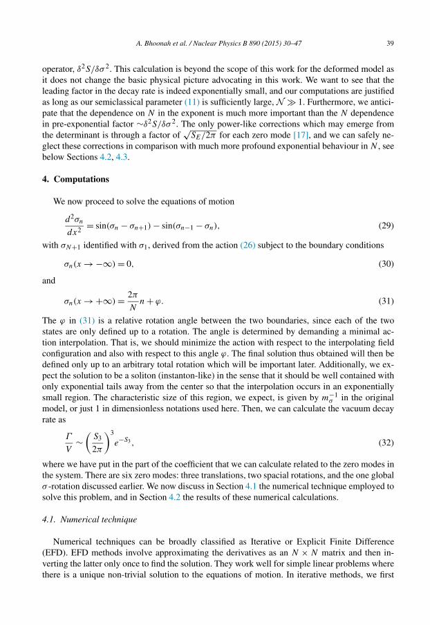
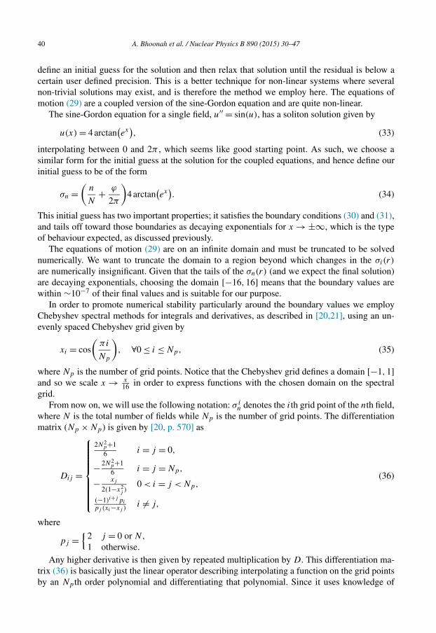
The first issue we address is the question about the favoured angle, ϕ, between the two bound-aries, (30) and (31). In order to find the angle we chose (arbitrarily) N = 7 and varied the angle in the range [−π, π] − 8π/7, and look at the action S1 as a function of ϕ. The results of that simulation are plotted in Fig. 1. The center point on the plot, −8π/7, may seem odd, but it is the value for ϕ which leads to a maximally symmetric solution, so it is very believable minimum for the potential, and indeed this is what we see. The solution for the minimal σ field configuration corresponding to ϕ = −8π/7 is shown in Fig. 2 across the domain wall. Extending these results to arbitrary N we set

ϕ = −π

(N + 1

N

), (39)

which just ensures that the solution we look for is maximally symmetric in the same sense as the fields in Fig. 2, basically that σn = −σN+1−n. We have checked that this choice of ϕ, (39), does in fact lead to the lowest action configuration for N = 20 and N = 35 with results much like those shown in Fig. 1 for N = 7, so we are comfortable with our assumption.

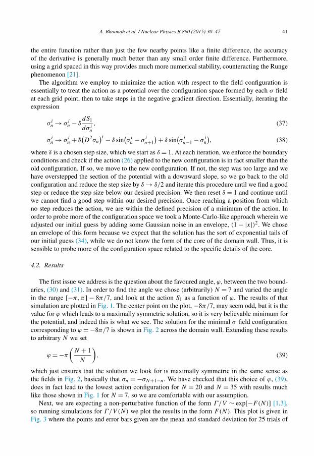
Next, we are expecting a non-perturbative function of the form Γ/V ∼ exp[−F(N)] [1,3], so running simulations for Γ/V (N) we plot the results in the form F(N). This plot is given in Fig. 3 where the points and error bars given are the mean and standard deviation for 25 trials of

42 A. Bhoonah et al. / Nuclear Physics B 890 (2015) 30–47

Fig. 1. A plot of some simulation data for the one-dimensional action (26) as a function of the angle ϕ between the boundary conditions done for N = 7.

Fig. 2. A plot of some simulation data for the σ field configuration plotted across the domain wall done for N = 7.

our simulation at each N between 15 and 75 using 312 Chebyshev grid points; it is shown on a log–log scale to emphasize the power law behaviour of F(N).

The particular fit parameters are given for completeness but should not be regarded as terribly important. In fact, the most important result for the present analysis is that the computations are

A. Bhoonah et al. / Nuclear Physics B 890 (2015) 30–47 43

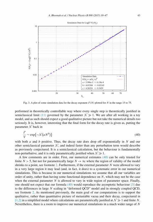
Fig. 3. A plot of some simulation data for the decay exponent F(N) plotted for N in the range 15 to 75.

performed in theoretically controllable way where every single step is theoretically justified in semiclassical limit (11) governed by the parameter N � 1. We are after all working in a toy model, and as such should expect a good qualitative picture but not take the numerical details too seriously. It is, however, interesting that the final form for the decay rate is given as, putting the parameter N back in

Γ

V∼ exp

{−N(aNb

)}(40)

with both a and b positive. Thus, the decay rate does drop off exponentially in N and our other semiclassical parameter N , and indeed faster than any perturbation term would describe as previously conjectured. It is a semiclassical calculation, but the behaviour is fundamentally non-perturbative, and it is only parametrically justified when N � 1.

A few comments are in order. First, our numerical estimates (40) can be only trusted for finite N > 5, but not for parametrically large N → ∞ where the region of validity of the model shrinks to a point, see footnote 2. Furthermore, if the external parameter N were allowed to vary in a very large region it may lead (and, in fact, it does) to a systematic error in our numerical simulations. This is because in our numerical simulations we assume that all our variables are order of unity, rather than having some functional dependence on N , which may not be the case when the external parameter N is allowed to vary in wide region of parameter space. Finally, one should not expect that our formula (40) would reproduce the asymptotic behaviour [3] due to the differences in large N scaling in “deformed QCD” model and in strongly coupled QCD, see footnote 2. As mentioned previously, the main goal of our computations is to support the qualitative, rather than quantitative picture of metastable vacua and their decay, conjectured in [1,2] in a simplified model where calculations are parametrically justified at N � 1 and finite N . Nevertheless, there is a room to improve our numerical simulations in a much wider range of N

44 A. Bhoonah et al. / Nuclear Physics B 890 (2015) 30–47

as a result of the recent analysis [31] in which the asymptotic expression at N → ∞ has been analytically computed. These improvements are discussed in the next section.

4.3. Improved results

Recently, an analytical analysis of the asymptotic behaviour of this calculation, inspired by the above numerical results, has been carried out [31] with the asymptotic expression for the decay rate per unit volume given by

Γ

V∼ exp

[−N 256N7/2

9√

3π(π − θ)2

]. (41)

The asymptotic expression (41) gives us a hint about how to produce a better estimate for the decay rate for very large N � 1 in comparison with our naive numerical results presented in Section 4.2 above, wherein we assumed that parameter N is not allowed to vary in an extended region of parameter space.

Indeed, the analysis in [31] suggests the specific reason for the disparity between the asymp-totic expression and the numerical results shown in Fig. 3 for large N . Mainly, the asymptotic guess solution is given by

σn(x) =(

4n

N− 2

)arctan

[exp

(−2

√3

Nx

)], (42)

which has a size ∼√N changing with the parameter N . Our guess solution (34) does not scale

with N and so becomes an increasingly bad guess at asymptotically larger N , such that our numerical solver becomes increasingly likely to find some other local minimum of the action. Furthermore, our integration domain was fixed for all N as we did not even attempt to consider any large variations with N in our analysis in Section 4.2. When we allow the external parameter N to become “large”, the true minimal action interpolating trajectory eventually will not “fit” in the finite size numerical grid which we fixed for all N . Essentially, forcing boundary conditions on too small a domain also forces a higher action local minimum as N increases. This is pre-cisely the mechanism by which a systematic error is introduced into the numerical simulations as a result of large variation in the external parameter N , as suggested in the previous section after (40).

Fortunately, the analytical expression (42) which is valid for asymptotically large N suggests a simple fix to improve our numerical solution at higher N by explicitly taking into account the variation of the trajectory size with this parameter. Technically, we can allow the integration domain to scale ∼√

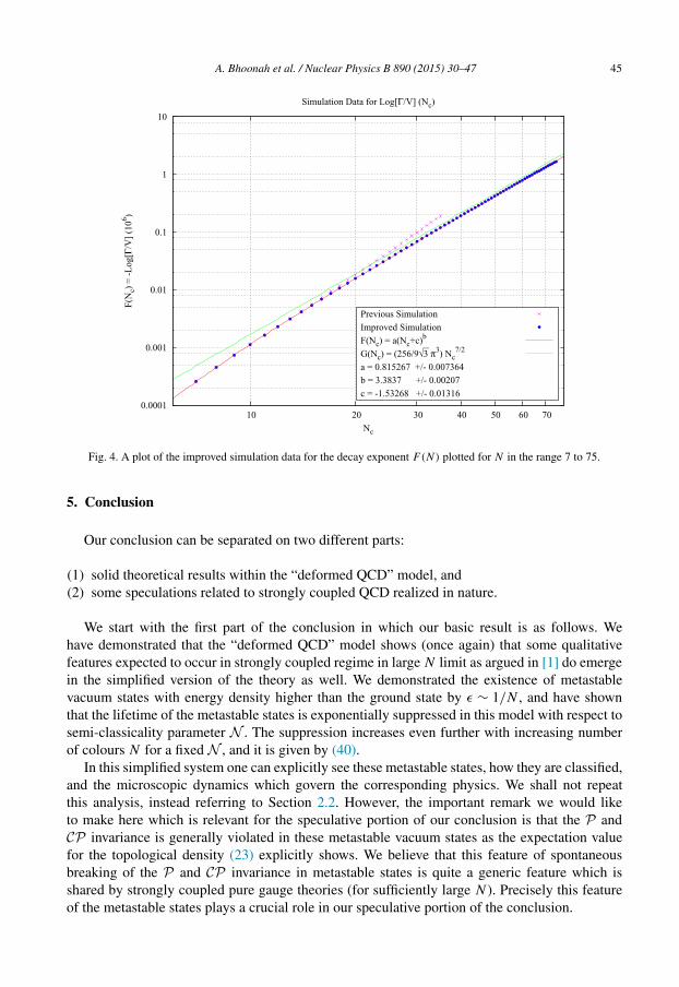
N , and start with the asymptotic guess (42) in which the large parameter Nexplicitly enters, as the initial guess for the “improved” numerical algorithm. Again, we added some Gaussian noise to get an ensemble of 25 initial guesses for each N and relaxed them as described in Section 4.1 to arrive at a minimum of the action. These improved results are shown in Fig. 4 plotted along with the asymptotic expression for the decay rate and the first few points from the original simulations in Section 4.2. They reproduce the previous results for finite N ≤ 15 and approach the asymptotic result (41) given in [31] from below for large N . Numerically, the asymptotic expression (41), which is formally valid at N → ∞, describes our improved simulation data sufficiently well (with accuracy better than 10%) only at large N ≥ 35.

A. Bhoonah et al. / Nuclear Physics B 890 (2015) 30–47 45

Fig. 4. A plot of the improved simulation data for the decay exponent F(N) plotted for N in the range 7 to 75.

5. Conclusion

Our conclusion can be separated on two different parts:

(1) solid theoretical results within the “deformed QCD” model, and(2) some speculations related to strongly coupled QCD realized in nature.

We start with the first part of the conclusion in which our basic result is as follows. We have demonstrated that the “deformed QCD” model shows (once again) that some qualitative features expected to occur in strongly coupled regime in large N limit as argued in [1] do emerge in the simplified version of the theory as well. We demonstrated the existence of metastable vacuum states with energy density higher than the ground state by ε ∼ 1/N , and have shown that the lifetime of the metastable states is exponentially suppressed in this model with respect to semi-classicality parameter N . The suppression increases even further with increasing number of colours N for a fixed N , and it is given by (40).

In this simplified system one can explicitly see these metastable states, how they are classified, and the microscopic dynamics which govern the corresponding physics. We shall not repeat this analysis, instead referring to Section 2.2. However, the important remark we would like to make here which is relevant for the speculative portion of our conclusion is that the P and CP invariance is generally violated in these metastable vacuum states as the expectation value for the topological density (23) explicitly shows. We believe that this feature of spontaneous breaking of the P and CP invariance in metastable states is quite a generic feature which is shared by strongly coupled pure gauge theories (for sufficiently large N ). Precisely this feature of the metastable states plays a crucial role in our speculative portion of the conclusion.

46 A. Bhoonah et al. / Nuclear Physics B 890 (2015) 30–47

Therefore, we now speculate that precisely this spontaneous symmetry breaking effect is re-sponsible for the asymmetries in event by event studies observed at the RHIC (Relativistic Heavy Ion Collider) and the LHC (Large Hadron Collider). To be more specific, the violation of local Pand CP symmetries has been the subject of intense studies for the last couple of years as a result of very interesting ongoing experiments at RHIC [22,23] and, more recently, at the LHC [24–27], see [29] for a recent review and introduction to the subject with a large number of references to original papers.

The main idea for explaining the observed asymmetries is to assume [28,29] that an effective θ(�x, t)ind = 0 is induced in the process of cooling of the system representing the high temperature quark–gluon plasma. In other words, the system in the process of cooling may spontaneously choose one or another state which is not the absolute minimum of the system corresponding to the θ = 0, but rather, some excited state, similar to the old idea when the disoriented chiral condensate can be formed as a result of heavy ion collisions. The key assumption is that this induced θ(�x, t)ind = 0 is coherent on a large scale of order of nuclei ∼10 fm, rather than on much smaller scale of order of 1 fm. If a state with 〈θ(�x, t)ind〉 = 0 is indeed induced, it implies a violation of the local P and CP symmetries on the same scales where θ(�x, t)ind = 0 is correlated. It may then generate a number of P and CP violating effects, such as Charge/Chiral Separation (CSE) and Chiral Magnetic (CME) Effects, see [29] for a recent review.

One of the critical questions for the applications of the CME to heavy ion collisions is a correlation length of the induced 〈θ(�x, t)ind〉 = 0. Why are these P odd domains large?

We would like to speculate that the crucial element in the understanding of this key question might be related to the metastable states which are the subject of the present work. To be more specific, we suggest that the system being originally formed at high temperature might be locked in one of these metastable states during the cooling stage.4 If this happens one should obviously expect a number of P and CP effects to occur coherently in the entire system characterized by a large scale of order the size of nuclei L � Λ−1

QCD. We therefore identify θ(�x, t)ind = 0 from [28]with the effective theta parameter 2π/N which enters (23) and which manifests a spontaneous violation of the P and CP symmetries in the system.

The presence of such long range order (which itself is a consequence of a spontaneous select-ing of a metastable vacuum state in the entire system during the cooling process) may explain why CME is operational in this system and how the asymmetry can be coherently accumulated from entire system. This identification would justify the effective Lagrangian approach advo-cated in [28,30] wherein θ(�x, t)ind is treated as slow background field with correlation length much larger than any conventional QCD fluctuations, L � Λ−1

QCD. It is important to emphasize that the P and CP symmetries are good symmetries of the fundamental QCD. As mentioned in footnote 4 the asymmetries can only be observed in heavy ion collisions in event by event anal-ysis when the system might be locked for sufficiently long period of time τ ∼ L/c � Λ−1

QCD in a metastable state in one collision with one specific sign for the topological density (23). Because the metastable states with opposite signs for the topological density operator (23) have the same energy, which state is chosen for a particular event is random and evenly distributed. Thus, it is clear that if one averages over large number of events, the asymmetry will be washed out as the probability to form these metastable states is identical and the lifetime for the two is the same

4 The P and CP symmetries, of course, are good symmetries in QCD. The probability to produce m = +1 state from Eq. (19) is identically the same as produce m = −1 state. Therefore, there will be no any P and CP violating effects if one averages over large number of events. However, one should expect some asymmetries if one analyzes the system on event by event basis, which is precisely the procedure used at RHIC and the LHC, see Ref. [29] for a recent review.

A. Bhoonah et al. / Nuclear Physics B 890 (2015) 30–47 47

as we mentioned in Section 2.2. However, in the event by event studies the asymmetry will be evident in the system. Apparently, this is precisely what has been observed, see the recent review paper [29] for the details.

Acknowledgements

E. Thomas would like to thank Michael Forbes and Darren Smyth for discussions related to the solving of nonlinear boundary value problems.

This research was supported in part by the Natural Sciences and Engineering Research Coun-cil of Canada.

References

[1] E. Witten, Ann. Phys. 128 (1980) 363.[2] E. Witten, Phys. Rev. Lett. 81 (1998) 2862, arXiv:hep-th/9807109.[3] M.A. Shifman, Phys. Rev. D 59 (1999) 021501, arXiv:hep-th/9809184.[4] E. Witten, Nucl. Phys. B 156 (1979) 269.[5] G. Veneziano, Nucl. Phys. B 159 (1979) 213.[6] P. Di Vecchia, G. Veneziano, Nucl. Phys. B 171 (1980) 253.[7] M. Ünsal, L.G. Yaffe, Phys. Rev. D 78 (2008) 065035, arXiv:0803.0344 [hep-th].[8] E. Thomas, A.R. Zhitnitsky, Phys. Rev. D 85 (2012) 044039, arXiv:1109.2608 [hep-th].[9] M. Unsal, Phys. Rev. D 86 (2012) 105012, arXiv:1201.6426 [hep-th].

[10] I. Horvath, A. Alexandru, J.B. Zhang, Y. Chen, S.J. Dong, T. Draper, K.F. Liu, N. Mathur, et al., Phys. Lett. B 617 (2005) 49–59, arXiv:hep-lat/0504005.

[11] E.-M. Ilgenfritz, K. Koller, Y. Koma, G. Schierholz, T. Streuer, V. Weinberg, Phys. Rev. D 76 (2007) 034506, arXiv:0705.0018 [hep-lat].

[12] E.-M. Ilgenfritz, D. Leinweber, P. Moran, K. Koller, G. Schierholz, V. Weinberg, Phys. Rev. D 77 (2008) 074502, arXiv:0801.1725 [hep-lat];E.-M. Ilgenfritz, D. Leinweber, P. Moran, K. Koller, G. Schierholz, V. Weinberg, Phys. Rev. D 77 (2008) 099902 (Erratum).

[13] F. Bruckmann, F. Gruber, N. Cundy, A. Schafer, T. Lippert, Phys. Lett. B 707 (2012) 278, arXiv:1107.0897 [hep-lat].[14] A.R. Zhitnitsky, Ann. Phys. 336 (2013) 462, arXiv:1301.7072 [hep-ph].[15] A.R. Zhitnitsky, Phys. Rev. D 88 (10) (2013) 105029, arXiv:1308.1960 [hep-th].[16] I.Y. Kobzarev, L.B. Okun, M.B. Voloshin, Sov. J. Nucl. Phys. 20 (1975) 644;

I.Y. Kobzarev, L.B. Okun, M.B. Voloshin, Yad. Fiz. 20 (1974) 1229.[17] S. Coleman, Phys. Rev. D 15 (1977) 2929.[18] C.G. Callan, S. Coleman, Phys. Rev. D 16 (1977) 1762.[19] E. Thomas, A.R. Zhitnitsky, Phys. Rev. D 87 (8) (2013) 085027, arXiv:1208.2030 [hep-ph].[20] J. Boyd, Chebyshev and Fourier Spectral Methods, 2nd ed., General Publishing Company, Toronto, 2001.[21] L. Trefethen, Spectral Methods in Matlab, Society for Industrial and Applied Mathematics, Philadelphia, 2000.[22] B.I. Abelev, et al., STAR Collaboration, Phys. Rev. C 81 (2010) 054908, arXiv:0909.1717 [nucl-ex].[23] G. Wang, STAR Collaboration, arXiv:1210.5498 [nucl-ex].[24] I. Selyuzhenkov, ALICE Collaboration, PoS WPCF 2011 (2011) 044, arXiv:1203.5230 [nucl-ex].[25] B. Abelev, et al., ALICE Collaboration, arXiv:1207.0900 [nucl-ex].[26] S.A. Voloshin, ALICE Collaboration, arXiv:1211.5680 [nucl-ex].[27] I. Selyuzhenkov, arXiv:1212.5489 [nucl-ex].[28] D. Kharzeev, A. Zhitnitsky, Nucl. Phys. A 797 (2007) 67, arXiv:0706.1026 [hep-ph].[29] D.E. Kharzeev, Prog. Part. Nucl. Phys. 75 (2014) 133, arXiv:1312.3348 [hep-ph].[30] A.R. Zhitnitsky, Nucl. Phys. A 886 (2012) 17, arXiv:1201.2665 [hep-ph].[31] X. Li, M.B. Voloshin, arXiv:1408.3054 [hep-th].