Maxwell Equations; Magnetism of Matter · Ampere-Maxwell Law Ampere’s law, gives the magnetic...

Maxwell Equations; Magnetism of Matter

Chapter 32

Copyright © 2014 John Wiley & Sons, Inc. All rights reserved.

32-1 Gauss’ Law for Magnetic Fields

32.01 Identify that the simplest magnetic structure is a magnetic dipole.

32.02 Calculate the magnetic flux ϕ through a surface by integrating the dot product of the magnetic field vector B and the area vector dA (for patch elements) over the surface.

32.03 Identify that the net magnetic flux through a Gaussian surface (which is a closed surface) is zero.

Learning Objectives

© 2014 John Wiley & Sons, Inc. All rights reserved.

32-1 Gauss’ Law for Magnetic Fields

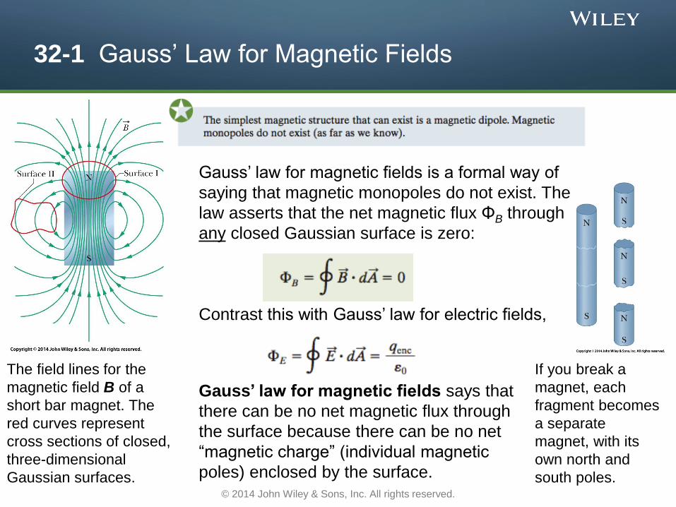
Gauss’ law for magnetic fields is a formal way of

saying that magnetic monopoles do not exist. The

law asserts that the net magnetic flux ΦB through

any closed Gaussian surface is zero:

Contrast this with Gauss’ law for electric fields,

If you break a

magnet, each

fragment becomes

a separate

magnet, with its

own north and

south poles.

The field lines for the

magnetic field B of a

short bar magnet. The

red curves represent

cross sections of closed,

three-dimensional

Gaussian surfaces.

Gauss’ law for magnetic fields says that

there can be no net magnetic flux through

the surface because there can be no net

“magnetic charge” (individual magnetic

poles) enclosed by the surface. © 2014 John Wiley & Sons, Inc. All rights reserved.

32-2 Induced Magnetic Fields

32.04 Identify that a changing electric flux induces a magnetic field.

32.05 Apply Maxwell’s law of induction to relate the magnetic field induced around a closed loop to the rate of change of electric flux encircled by the loop.

32.06 Draw the field lines for an induced magnetic field inside a capacitor with parallel circular plates that are being charged, indicating the orientations of the vectors for the electric field and the magnetic field.

32.07 For the general situation in which magnetic fields can be induced, apply the Ampere–Maxwell (combined) law.

Learning Objectives



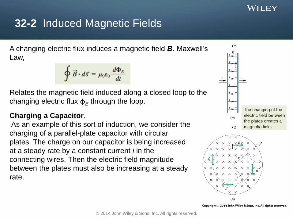
A changing electric flux induces a magnetic field B. Maxwell’s

Law,

Relates the magnetic field induced along a closed loop to the

changing electric flux ϕE through the loop.

Charging a Capacitor.

As an example of this sort of induction, we consider the

charging of a parallel-plate capacitor with circular

plates. The charge on our capacitor is being increased

at a steady rate by a constant current i in the

connecting wires. Then the electric field magnitude

between the plates must also be increasing at a steady

rate.



A changing electric flux induces a magnetic field B. Maxwell’s

Law,

Relates the magnetic field induced along a closed loop to the

changing electric flux ϕE through the loop.

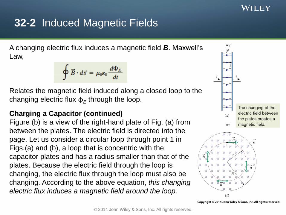
Charging a Capacitor (continued)

Figure (b) is a view of the right-hand plate of Fig. (a) from

between the plates. The electric field is directed into the

page. Let us consider a circular loop through point 1 in

Figs.(a) and (b), a loop that is concentric with the

capacitor plates and has a radius smaller than that of the

plates. Because the electric field through the loop is

changing, the electric flux through the loop must also be

changing. According to the above equation, this changing

electric flux induces a magnetic field around the loop.



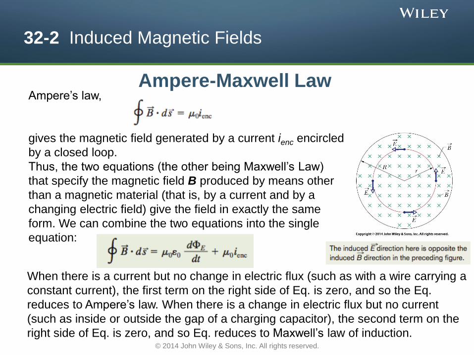
Ampere-Maxwell Law Ampere’s law,

gives the magnetic field generated by a current ienc encircled

by a closed loop.

Thus, the two equations (the other being Maxwell’s Law)

that specify the magnetic field B produced by means other

than a magnetic material (that is, by a current and by a

changing electric field) give the field in exactly the same

form. We can combine the two equations into the single

equation:

When there is a current but no change in electric flux (such as with a wire carrying a

constant current), the first term on the right side of Eq. is zero, and so the Eq.

reduces to Ampere’s law. When there is a change in electric flux but no current

(such as inside or outside the gap of a charging capacitor), the second term on the

right side of Eq. is zero, and so Eq. reduces to Maxwell’s law of induction. © 2014 John Wiley & Sons, Inc. All rights reserved.

32-3 Displacement Current

32.08 Identify that in the Ampere–Maxwell law, the contribution to the induced magnetic field by the changing electric flux can be attributed to a fictitious current (“displacement current”) to simplify the expression.

32.09 Identify that in a capacitor that is being charged or discharged, a displacement current is said to be spread uniformly over the plate area, from one plate to the other.

32.10 Apply the relationship between the rate of change of an electric flux and the associated displacement current.

32.11 For a charging or discharging capacitor, relate the amount of displacement current to the amount of actual current and identify that the displacement current exists only when the electric field within the capacitor is changing.

32.12 Mimic the equations for the magnetic field inside and outside a wire with real current to write (and apply) the equations for the magnetic field inside and outside a region of displacement current.

Learning Objectives



32.13 Apply the Ampere–Maxwell law to calculate the magnetic field of a real current and a displacement current.

32.14 For a charging or discharging capacitor with parallel circular plates, draw the magnetic field lines due to the displacement current.

32.15 List Maxwell’s equations and the purpose of each.

Learning Objectives (Contd.)



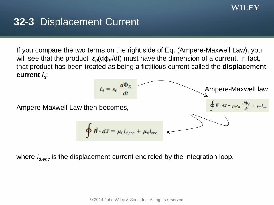
If you compare the two terms on the right side of Eq. (Ampere-Maxwell Law), you

will see that the product ε0(dϕE/dt) must have the dimension of a current. In fact,

that product has been treated as being a fictitious current called the displacement

current id:

Ampere-Maxwell Law then becomes,

where id,enc is the displacement current encircled by the integration loop.

Ampere-Maxwell law



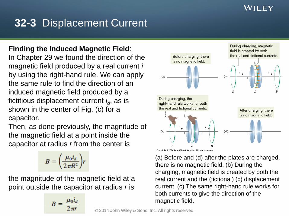
(a) Before and (d) after the plates are charged,

there is no magnetic field. (b) During the

charging, magnetic field is created by both the

real current and the (fictional) (c) displacement

current. (c) The same right-hand rule works for

both currents to give the direction of the

magnetic field.

Finding the Induced Magnetic Field:

In Chapter 29 we found the direction of the

magnetic field produced by a real current i

by using the right-hand rule. We can apply

the same rule to find the direction of an

induced magnetic field produced by a

fictitious displacement current id, as is

shown in the center of Fig. (c) for a

capacitor.

Then, as done previously, the magnitude of

the magnetic field at a point inside the

capacitor at radius r from the center is

the magnitude of the magnetic field at a

point outside the capacitor at radius r is



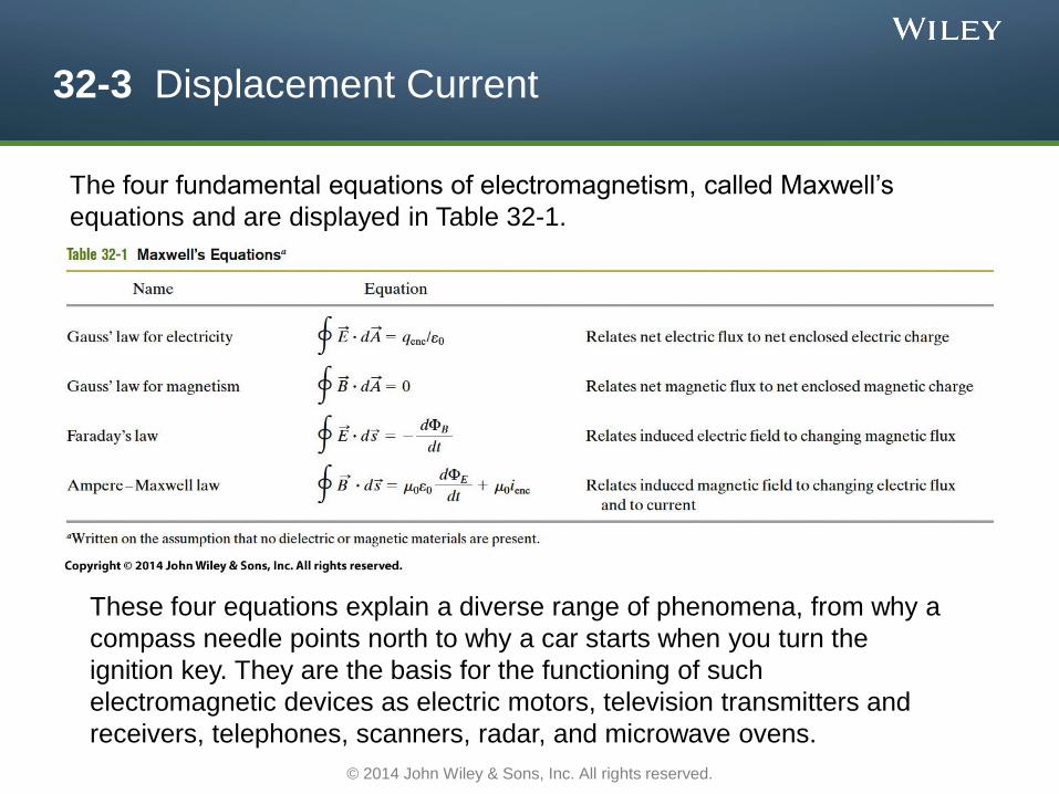
The four fundamental equations of electromagnetism, called Maxwell’s

equations and are displayed in Table 32-1.

These four equations explain a diverse range of phenomena, from why a

compass needle points north to why a car starts when you turn the

ignition key. They are the basis for the functioning of such

electromagnetic devices as electric motors, television transmitters and

receivers, telephones, scanners, radar, and microwave ovens.


32-4 Magnets

32.16 Identify lodestones.

32.17 In Earth’s magnetic field, identify that the field is approximately that of a dipole and also identify in which hemisphere the north geomagnetic pole is located.

32.18 Identify field declination and field inclination.

Learning Objectives


32-4 Magnets

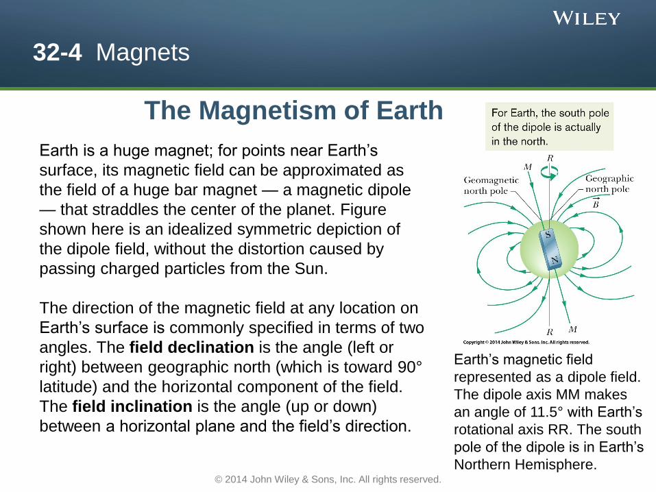
Earth is a huge magnet; for points near Earth’s

surface, its magnetic field can be approximated as

the field of a huge bar magnet — a magnetic dipole

— that straddles the center of the planet. Figure

shown here is an idealized symmetric depiction of

the dipole field, without the distortion caused by

passing charged particles from the Sun.

The direction of the magnetic field at any location on

Earth’s surface is commonly specified in terms of two

angles. The field declination is the angle (left or

right) between geographic north (which is toward 90°

latitude) and the horizontal component of the field.

The field inclination is the angle (up or down)

between a horizontal plane and the field’s direction.

Earth’s magnetic field

represented as a dipole field.

The dipole axis MM makes

an angle of 11.5° with Earth’s

rotational axis RR. The south

pole of the dipole is in Earth’s

Northern Hemisphere.

The Magnetism of Earth


32-5 Magnetism and Electrons

32.19 Identify that a spin angular momentum S (usually simply called spin) and a spin magnetic dipole moment μs are intrinsic properties of electrons (and also protons and neutrons).

32.20 Apply the relationship between the spin vector S and the spin magnetic dipole moment vector μs.

32.21 Identify that S and μs cannot be observed (measured); only their components on an axis of measurement (usually called the z axis) can be observed.

32.22 Identify that the observed components Sz and μs,z are quantized and explain what that means.

32.23 Apply the relationship between the component Sz and the spin magnetic quantum number ms, specifying the allowed values of ms.

32.24 Distinguish spin up from spin down for the spin orientation of an electron.

32.25 Determine the z components μs,z of the spin magnetic dipole moment, both as a value and in terms of the Bohr magneton μB.

Learning Objectives



32.26 If an electron is in an external magnetic field, determine the orientation energy U of its spin magnetic dipole moment μs.

32.27 Identify that an electron in an atom has an orbital angular momentum L and an orbital magnetic dipole moment μorb.

32.28 Apply the relationship between the orbital angular momentum L and the orbital magnetic dipole moment μorb.

32.29 Identity that L and μorb cannot be observed but their components Lorb,z and μorb,z on a z (measurement) axis can.

32.30 Apply the relationship between the component Lorb,z of the orbital angular momentum and the orbital magnetic quantum number ml, specifying the allowed values of ml.

32.31 Determine the z components μorb,z of the orbital magnetic dipole moment, both as a value and in terms of the Bohr magneton μB.




32.32 If an atom is in an external magnetic field, determine the orientation energy U of the orbital magnetic dipole moment μorb.

32.33 Calculate the magnitude of the magnetic moment of a charged particle moving in a circle or a ring of uniform charge rotating like a merry-go-round at a constant angular speed around a central axis.

32.34 Explain the classical loop model for an orbiting electron and the forces on such a loop in a non-uniform magnetic field.

32.35 Distinguish among diamagnetism, paramagnetism, and ferromagnetism.




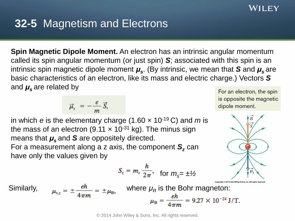
Spin Magnetic Dipole Moment. An electron has an intrinsic angular momentum

called its spin angular momentum (or just spin) S; associated with this spin is an

intrinsic spin magnetic dipole moment μs. (By intrinsic, we mean that S and μs are

basic characteristics of an electron, like its mass and electric charge.) Vectors S

and μs are related by

in which e is the elementary charge (1.60 × 10-19 C) and m is

the mass of an electron (9.11 × 10-31 kg). The minus sign

means that μs and S are oppositely directed.

For a measurement along a z axis, the component Sz can

have only the values given by

for ms= ±½

Similarly, where μB is the Bohr magneton:



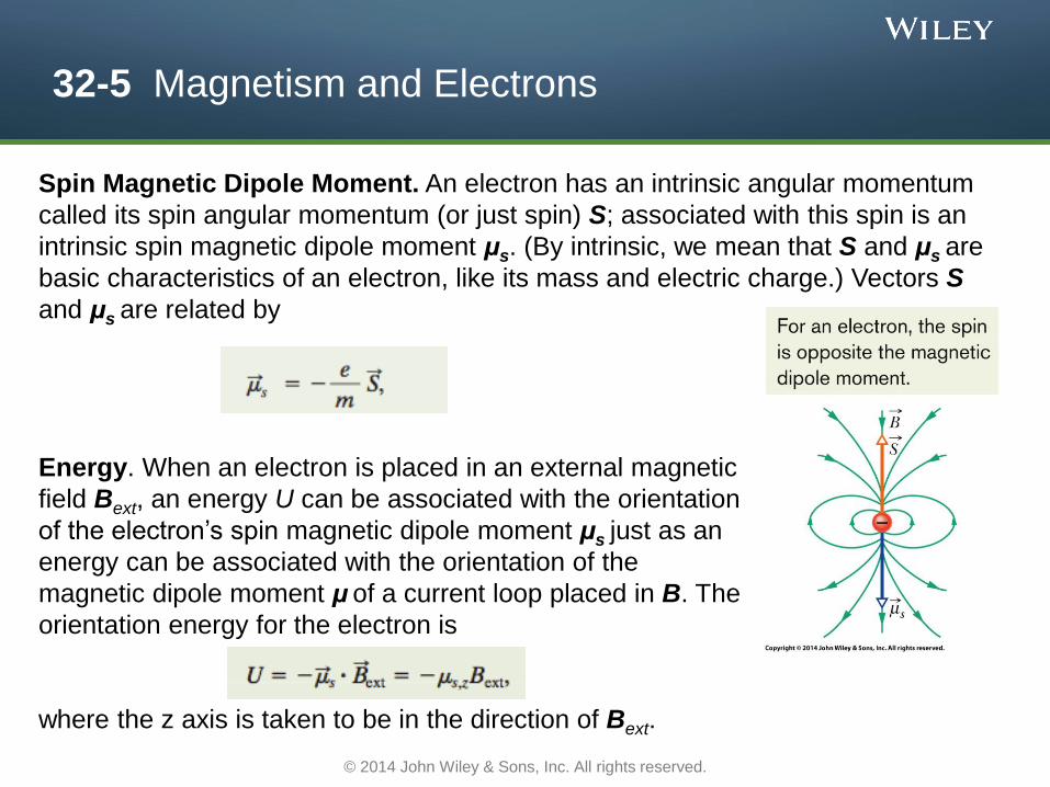
Spin Magnetic Dipole Moment. An electron has an intrinsic angular momentum

called its spin angular momentum (or just spin) S; associated with this spin is an

intrinsic spin magnetic dipole moment μs. (By intrinsic, we mean that S and μs are

basic characteristics of an electron, like its mass and electric charge.) Vectors S

and μs are related by

Energy. When an electron is placed in an external magnetic

field Bext, an energy U can be associated with the orientation

of the electron’s spin magnetic dipole moment μs just as an

energy can be associated with the orientation of the

magnetic dipole moment μ of a current loop placed in B. The

orientation energy for the electron is

where the z axis is taken to be in the direction of Bext.



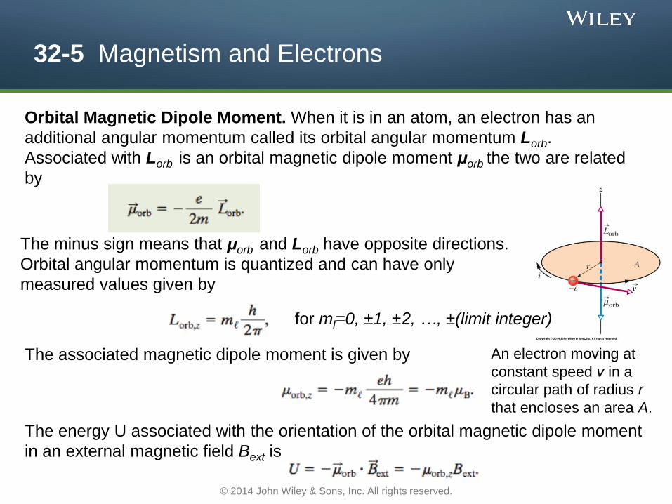
Orbital Magnetic Dipole Moment. When it is in an atom, an electron has an

additional angular momentum called its orbital angular momentum Lorb.

Associated with Lorb is an orbital magnetic dipole moment μorb the two are related

by

The minus sign means that μorb and Lorb have opposite directions.

Orbital angular momentum is quantized and can have only

measured values given by

for ml=0, ±1, ±2, …, ±(limit integer)

The associated magnetic dipole moment is given by

The energy U associated with the orientation of the orbital magnetic dipole moment

in an external magnetic field Bext is

An electron moving at

constant speed v in a

circular path of radius r

that encloses an area A.


32-6 Diamagnetism

32.36 For a diamagnetic sample placed in an external magnetic field, identify that the field produces a magnetic dipole moment in the sample, and identify the relative orientations of that moment and the field.

32.37 For a diamagnetic sample in a non-uniform magnetic field, describe the force on the sample and the resulting motion.

Learning Objectives


32-6 Diamagnetism

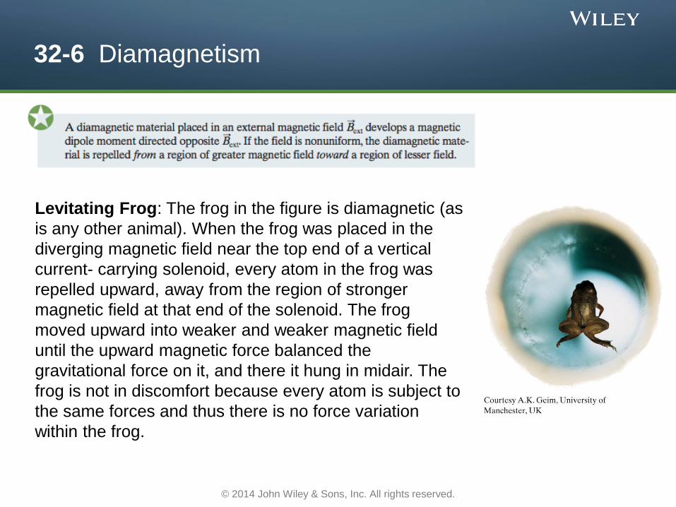
Levitating Frog: The frog in the figure is diamagnetic (as

is any other animal). When the frog was placed in the

diverging magnetic field near the top end of a vertical

current- carrying solenoid, every atom in the frog was

repelled upward, away from the region of stronger

magnetic field at that end of the solenoid. The frog

moved upward into weaker and weaker magnetic field

until the upward magnetic force balanced the

gravitational force on it, and there it hung in midair. The

frog is not in discomfort because every atom is subject to

the same forces and thus there is no force variation

within the frog.


32-7 Paramagnetism

32.38 For a paramagnetic sample placed in an external magnetic field, identify the relative orientations of the field and the sample’s magnetic dipole moment.

32.39 For a paramagnetic sample in a non-uniform magnetic field, describe the force on the sample and the resulting motion.

32.40 Apply the relationship between a sample’s magnetization M, its measured magnetic moment, and its volume.

32.41 Apply Curie’s law to relate a sample’s magnetization M to its temperature T, its Curie constant C, and the magnitude B of the external field.

32.42 Given a magnetization curve for a paramagnetic sample, relate the extent of the magnetization for a given magnetic field and temperature.

32.43 For a paramagnetic sample at a given temperature and in a given magnetic field, compare the energy associated with the dipole orientations and the thermal motion.

Learning Objectives


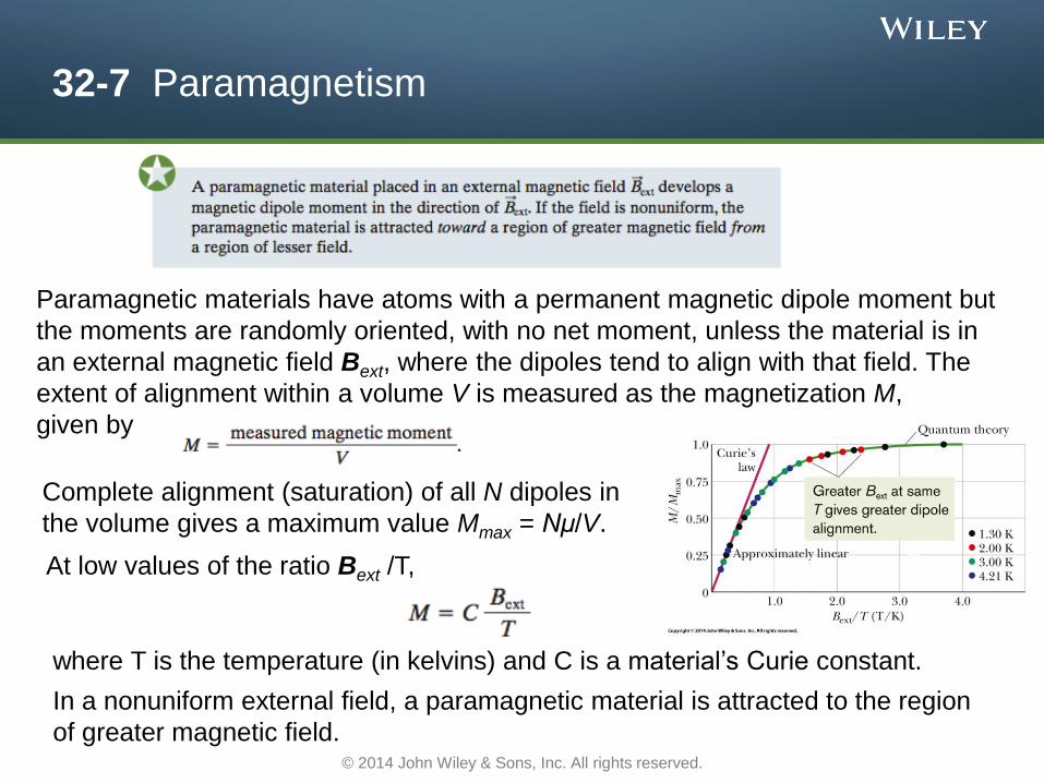
32-7 Paramagnetism

Paramagnetic materials have atoms with a permanent magnetic dipole moment but

the moments are randomly oriented, with no net moment, unless the material is in

an external magnetic field Bext, where the dipoles tend to align with that field. The

extent of alignment within a volume V is measured as the magnetization M,

given by

Complete alignment (saturation) of all N dipoles in

the volume gives a maximum value Mmax = Nμ/V.

At low values of the ratio Bext /T,

where T is the temperature (in kelvins) and C is a material’s Curie constant.

In a nonuniform external field, a paramagnetic material is attracted to the region

of greater magnetic field. © 2014 John Wiley & Sons, Inc. All rights reserved.

32-8 Ferromagnetism

32.44 Identify that ferromagnetism is due to a quantum mechanical interaction called exchange coupling.

32.45 Explain why ferromagnetism disappears when the temperature exceeds the material’s Curie temperature.

32.46 Apply the relationship between the magnetization of a ferromagnetic sample and the magnetic moment of its atoms.

32.47 For a ferromagnetic sample at a given temperature and in a given magnetic field, compare the energy associated with the dipole orientations and the thermal motion.

32.48 Describe and sketch a Rowland ring.

32.49 Identify magnetic domains.

32.50 For a ferromagnetic sample placed in an external magnetic field, identify the relative orientations of the field and the magnetic dipole moment.

Learning Objectives


32-8 Ferromagnetism

32.51 Identify the motion of a ferromagnetic sample in a non-uniform field.

32.52 For a ferromagnetic object placed in a uniform magnetic field, calculate the torque and orientation energy.

32.53 Explain hysteresis and a hysteresis loop.

32.54 Identify the origin of lodestones.



32-8 Ferromagnetism

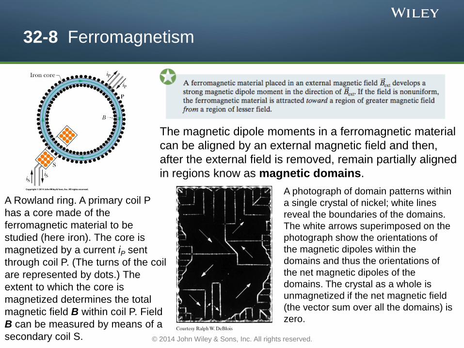
A Rowland ring. A primary coil P

has a core made of the

ferromagnetic material to be

studied (here iron). The core is

magnetized by a current iP sent

through coil P. (The turns of the coil

are represented by dots.) The

extent to which the core is

magnetized determines the total

magnetic field B within coil P. Field

B can be measured by means of a

secondary coil S.

The magnetic dipole moments in a ferromagnetic material

can be aligned by an external magnetic field and then,

after the external field is removed, remain partially aligned

in regions know as magnetic domains.

A photograph of domain patterns within

a single crystal of nickel; white lines

reveal the boundaries of the domains.

The white arrows superimposed on the

photograph show the orientations of

the magnetic dipoles within the

domains and thus the orientations of

the net magnetic dipoles of the

domains. The crystal as a whole is

unmagnetized if the net magnetic field

(the vector sum over all the domains) is

zero.


32-8 Ferromagnetism

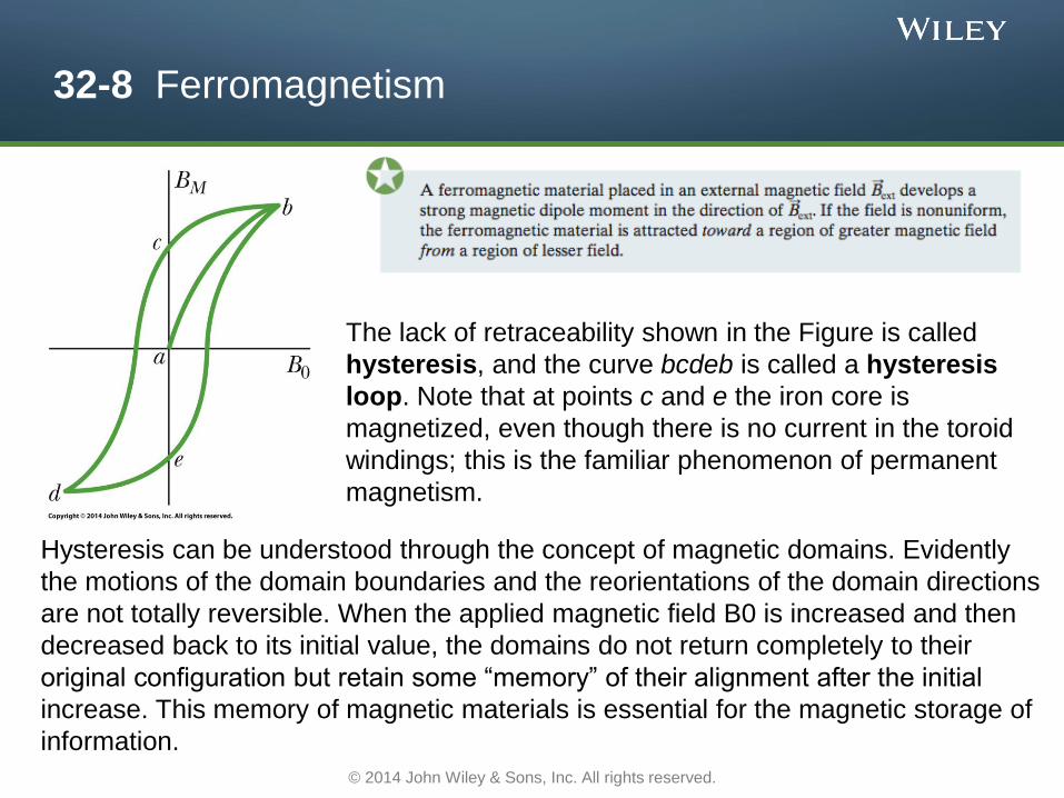
The lack of retraceability shown in the Figure is called

hysteresis, and the curve bcdeb is called a hysteresis

loop. Note that at points c and e the iron core is

magnetized, even though there is no current in the toroid

windings; this is the familiar phenomenon of permanent

magnetism.

Hysteresis can be understood through the concept of magnetic domains. Evidently

the motions of the domain boundaries and the reorientations of the domain directions

are not totally reversible. When the applied magnetic field B0 is increased and then

decreased back to its initial value, the domains do not return completely to their

original configuration but retain some “memory” of their alignment after the initial

increase. This memory of magnetic materials is essential for the magnetic storage of

information.


32 Summary

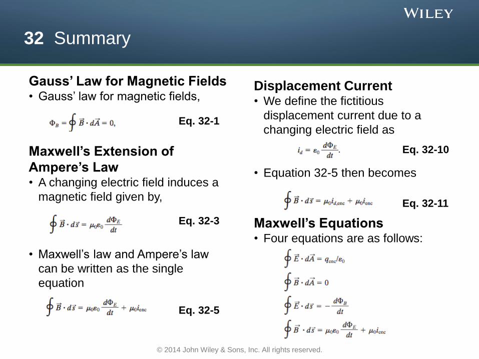
Gauss’ Law for Magnetic Fields • Gauss’ law for magnetic fields,

Eq. 32-1

Displacement Current • We define the fictitious

displacement current due to a

changing electric field as

• Equation 32-5 then becomes

Eq. 32-10 Maxwell’s Extension of

Ampere’s Law • A changing electric field induces a

magnetic field given by,

• Maxwell’s law and Ampere’s law

can be written as the single

equation

Eq. 32-3

Eq. 32-5

Eq. 32-11

Maxwell’s Equations • Four equations are as follows:


32 Summary

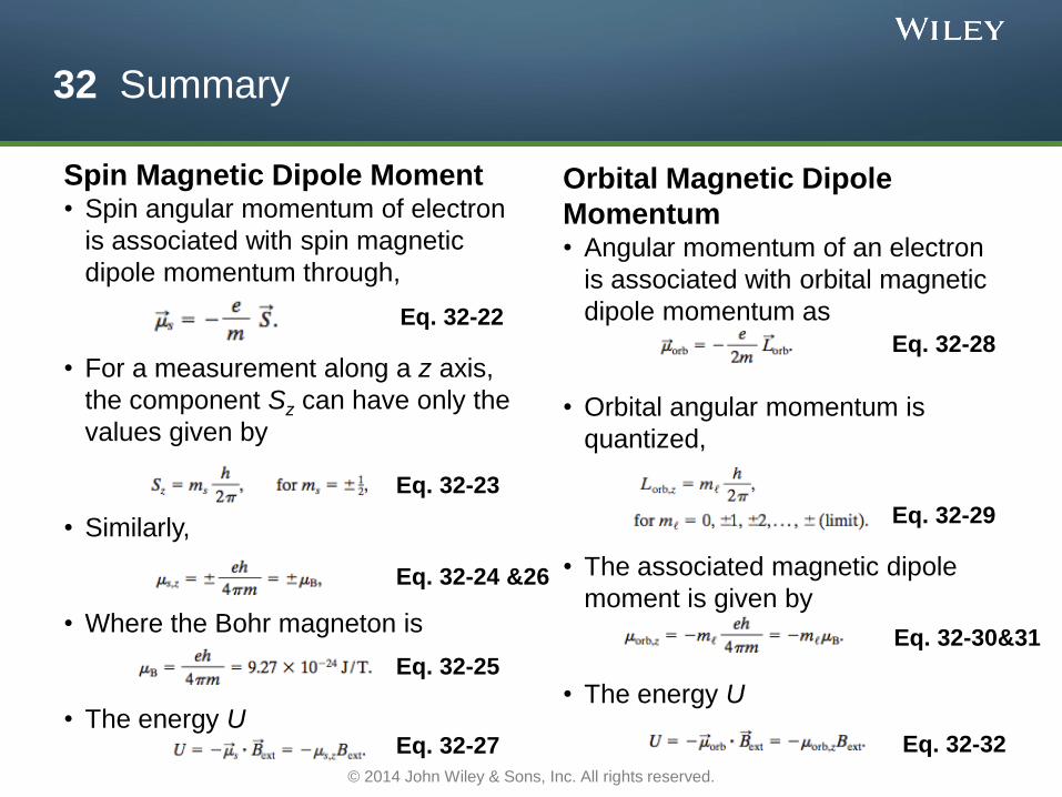
Spin Magnetic Dipole Moment • Spin angular momentum of electron

is associated with spin magnetic

dipole momentum through,

• For a measurement along a z axis,

the component Sz can have only the

values given by

• Similarly,

• Where the Bohr magneton is

• The energy U

Eq. 32-22

Orbital Magnetic Dipole

Momentum • Angular momentum of an electron

is associated with orbital magnetic

dipole momentum as

• Orbital angular momentum is

quantized,

• The associated magnetic dipole

moment is given by

• The energy U

Eq. 32-28

Eq. 32-23

Eq. 32-24 &26

Eq. 32-29

Eq. 32-25

Eq. 32-27

Eq. 32-30&31

Eq. 32-32


32 Summary

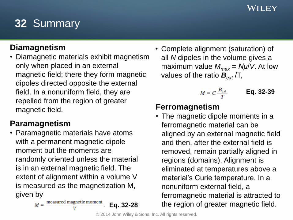
Diamagnetism • Diamagnetic materials exhibit magnetism

only when placed in an external

magnetic field; there they form magnetic

dipoles directed opposite the external

field. In a nonuniform field, they are

repelled from the region of greater

magnetic field.

• Complete alignment (saturation) of

all N dipoles in the volume gives a

maximum value Mmax = Nμ/V. At low

values of the ratio Bext /T,

Eq. 32-39

Eq. 32-28

Paramagnetism • Paramagnetic materials have atoms

with a permanent magnetic dipole

moment but the moments are

randomly oriented unless the material

is in an external magnetic field. The

extent of alignment within a volume V

is measured as the magnetization M,

given by

Ferromagnetism • The magnetic dipole moments in a

ferromagnetic material can be

aligned by an external magnetic field

and then, after the external field is

removed, remain partially aligned in

regions (domains). Alignment is

eliminated at temperatures above a

material’s Curie temperature. In a

nonuniform external field, a

ferromagnetic material is attracted to

the region of greater magnetic field.


Maxwell Equations; Magnetism of Matter · Ampere-Maxwell Law Ampere’s law, gives the magnetic...

Documents

Transcript of Maxwell Equations; Magnetism of Matter · Ampere-Maxwell Law Ampere’s law, gives the magnetic...