On Γ−Convergence of a Variational Model forLithium-Ion Batteries

Kerrek Stinsonkstinson@andrew.cmu.eduCarnegie Mellon University

March 31, 2020

Abstract

A singularly perturbed phase field model used to model lithium-ion batteries includingchemical and elastic effects is considered. The underlying energy is given by

Iε[u, c] :=

∫Ω

(1

εf(c) + ε‖∇c‖2 +

1

εC(e(u)− ce0) : (e(u)− ce0)

)dx,

where f is a double well potential, C is a symmetric positive definite fourth order tensor,c is the normalized lithium-ion density, and u is the material displacement. The integrandcontains elements close to those in energy functionals arising in both the theory of fluid-fluidand solid-solid phase transitions. For a strictly star-shaped, Lipschitz domain Ω ⊂ R2, it isproven that Γ− limε→0 Iε = I0, where I0 is finite only for pairs (u, c) such that f(c) = 0 andthe symmetrized gradient e(u) = ce0 almost everywhere. Furthermore, I0 is characterizedas the integral of an anisotropic interfacial energy density over sharp interfaces given bythe jumpset of c.

Key words: Gamma convergence, lithium-ion batteries, linear elasticityAMS Classifications: 74G65, 49J45, 74N99

1 Introduction

The lithium-ion battery is a fundamental tool in modern technology and the intertwined chal-lenge of harnessing renewable energy, with applications extending from mobile phones to hybridcars. In recognition of this importance, the 2019 Nobel Prize in Chemistry was awarded to Good-enough, Whittingham, and Yoshino for their pioneering works in the development of lithium-ionbatteries [1]. Motivated by the eminence of lithium-ion batteries, we study a mathematicalmodel that underlies their capacity. A prominent performance limitation of lithium-ion bat-teries is their short life-cycle resulting from the electrochemical processes governing the batterywhich induce phase transitions. Elaborating on this, during the process of charging, lithium-ionsintercalate into the host structure of the cathode. This intercalation is not homogeneous andundergoes phase separation, that is, lithium-ions form areas of high concentration and low con-centration with sharp phase transitions between these regions. These phase transitions induce astrain on the host material which, ultimately, leads to its degradation. Damage of the cathode’shost material leads to a decrease in battery performance and limited life-cycle (see [9], [22], andreferences therein).

Understanding the onset of phase transitions is, therefore, imperative to improving batteryperformance, and much work has been done in this direction. Contemporary paradigms formodeling lithium-ion batteries are moving towards the incorporation of phase field models, alsoknown as diffuse interface models (see, e.g., [43], [18], [5], [7], [41]). These phase field modelsare governed by global energy functionals, which have regular inputs (e.g. Sobolev functions).As noted in [9], the phase field field model is robust, allowing for electrochemically consistentmodels for the time evolution of lithium-ion batteries. Competing models include the shrinkingcore model and the sharp interface model; however, as noted in Burch et. al. [14], the shrinkingcore model fails to capture fundamental qualitative behavior. Furthermore, in [33] it is proposedthat the phase field model may provide a more accurate numerical analysis of the problem thanthe sharp interface model, which seeks to model the evolution of the phase boundary as a freeboundary problem (see [15]; see also [2], and references therein, for benefits of the phase fieldmodel).

In this paper we study a variational model introduced by Cogswell and Bazant in [18] (seealso [9], [44], [43], [13]). For a fixed domain Ω ⊂ R2, we consider a phase field model for whichthe free energy functional is given by

I[u, c,Ω] :=

∫Ω

(f(c) + ρ‖∇c‖2 + C(e(u)− ce0) : (e(u)− ce0)

)dz

withf(s) := ωs(1− s) +KT (s log(s) + (1− s) log(1− s)), s ∈ [0, 1]. (1.1)

Here c : Ω→ [0, 1] stands for the normalized density of lithium-ions, and u : Ω→ R2 represents

the material displacement with symmetrized gradient e(u) := ∇u+∇uT2

, ω ∈ R is a regular solutionparameter (enthalpy of mixing), e0 ∈ R2×2 is the lattice misfit, K > 0 is the Boltzman constant,T > 0 is the absolute temperature, ρ > 0 is a constant associated with interfacial energy scalingwith interface width (see [6], [34], [39], [12], and references therein), and C is a symmetric,

1

positive definite, fourth order tensor, that captures the material constants (stiffness). Note thetensor C is defined to be positive definite as follows

C : R2×2 → R2×2sym, C(ξ) : ξ > 0 for all ξ ∈ R2×2

sym with ξ 6= 0. (1.2)

Adding a constant and letting ρ := ε2, we rescale the functional by 1/ε to consider thecollection of functionals Iεε>0 on H1(Ω,R2)× L2(Ω, [0, 1]) defined as

Iε[u, c,Ω] :=∫Ω

(1εf(c) + ε‖∇c‖2 + 1

εC(e(u)− ce0) : (e(u)− ce0)

)dz (u, c) ∈ H1(Ω,R2)×H1(Ω, [0, 1]),

∞ otherwise,

(1.3)where

f(s) := f(s)− mint∈[0,1]

f(t), s ∈ [0, 1] (1.4)

is a well function. We wish to consider the asymptotic behavior of this collection of energiesas ε → 0 (i.e., when the interfacial width goes to 0). This analysis will, in some capacity,mathematically validate the numerical solutions witnessing phase separation for small interfacialwidths as seen by Bazant and Cogswell in [18].

To study the asymptotic behavior, we will use the notion of Γ−convergence, as introducedby De Giorgi in [32]. Γ−convergence was first used by Modica and Mortola in [38] to study theclass of functionals arising in the Cahn-Hilliard theory of fluid-fluid transitions given by

Eε[c,Ω] :=

∫Ω

(1

εW (c) + ε‖∇c‖2

)dz, c ∈ H1(Ω,R),

where W is a double well function and Ω ⊂ RN (see also the foundational work by Cahn andHilliard [16]). Herein, they showed that Γ − limε→0Eε = E0, where E0(c) := CPerΩ(c), withPerΩ(c), the perimeter in Ω of one of the phases of c, taken to be∞ if c is not of finite perimeter.See also [31], [8], [3], and references therein.

More recently, a variety of work has been directed at analyzing classes of functionals givenby

Fε[u,Ω] :=

∫Ω

(1

εW (∇u) + ε‖∇2u‖2

)dz, u ∈ H2(Ω,RN), (1.5)

with Ω ⊂ RN , which arise in the theory of solid-solid phase transitions [12]. Accounting for frameindifference in a geometrically nonlinear framework, it is necessary to consider W satisfying thewell condition W (G) = 0 if and only if G ∈ SO(N)A∪SO(N)B for matrices A,B ∈ RN×N , whereSO(N) is the special orthogonal group. To guarantee existence of nonaffine functions for whichthe limiting energy is finite, the wells must satisfy Hadamard’s rank-one compatibility conditiongiven by QA−B = a⊗ ν for some Q ∈ SO(N), and a, ν ∈ RN (see [6], [26]). As an initial stepin [19], Conti et. al. treat the case of a double well function W disregarding frame indifference,meaning W (G) = 0 if and only if G = A or G = B, concluding that Fεε>0 Γ−convergesto a functional reminiscent of F0 defined in (1.6). Convergence of a case intermediate to Eεand Fε is considered by Fonseca and Mantegazza [29] wherein the nonconvex integrand of Fε is

2

replaced by 1εW (u). Many promising results regarding convergence of Fε when it is the Eikonal

functional, that is W (G) := (1 − ‖G‖2)2, have been obtained, although the Γ−limit is still yetto be identified (see [24], [25]).

Restricted to a strictly star-shaped Lipschitz domain Ω ⊂ R2, Conti and Schweizer in [21]address the problem of frame indifference in a geometrically linear framework, that is whenW is invariant under the tangent space of SO(2) or, equivalently, satisfies the well condition

W (G) = 0 if and only if G+GT

2∈ A ∪ B. Conti and Schweizer conclude that the functionals

Fεε>0 Γ−converge to

F0[u,Ω] :=

∫Je(u)

k(ν) dH1 if e(u) ∈ BV (Ω, A,B),∞ otherwise,

(1.6)

where Je(u) is the associated jumpset with normal ν, and k(ν) is the effective anisotropic in-terfacial energy density. Again, the existence of displacement with non-constant symmetrizedgradient exactly on the two wells requires a rank-one connectivity property. To be precise, thereis some skew-symmetric matrix S such that A−B+S is rank one (see Proposition 2.3). Further-more, the condition that e(u) ∈ BV (Ω, A,B) forces considerable restriction on the functionsfor which F0[u] <∞. Specifically, each interface of Je(u) has a single normal (out of two choices)and extends to the boundary of Ω. Consequently u behaves like a laminate (see Theorem 3.2).

Furthermore in [20], with N = 2, Conti and Schweizer analyze the case of a geometricallynonlinear framework with a result analogous to the linear case. In order to extend this result tohigher dimensions, in [23] Davoli and Friedrich analyze the energy∫

Ω

(1

εW (∇u) + ε‖∇2u‖2 + η(ε)(‖∇2u‖2 − |∂2

Nu|2)

)dz, u ∈ H2(Ω,RN)

utilizing sophisticated rigidity results for incompatible vector fields (see [40], [17], [35]). Here, itis assumed that the two wells of W are 0 and SO(N)eN ⊗ eN . Furthermore, the last term in theenergy specifically penalizes change in the displacement orthogonal to eN , and it follows thatthere is a single relevant interfacial normal, eN . This is in contrast to the two possible interfacialnormals that arise in the analysis of Fεε>0 (see Theorem 3.2). Here η(ε) → ∞ as ε → 0,leaving the identification of the Γ−limit of Fεε>0 in arbitrary dimensions an open problem.

Looking towards applications to fracture mechanics, Bellettini et. al. [11] analyze Γ−convergenceof the energy functionals∫

Ω

(1

εφ(1/ε)φ(‖∇u‖) + ε3‖∇2u‖2

)dz, u ∈ H2(Ω,RN)

where φ : [0,∞) → [0,∞) is continuous, nondecreasing, has sublinear growth at infinity, andsatisfies φ−1(0) = 0. As noted by the authors, this energy may viewed as a special case of(1.5) where the wells of W are at 0 and ∞.

The integrand in the energy Iε bears clear similarities to the integrands of both functionalsEε and Fε. In our analysis of the Γ−convergence of the functionals Iε, we will use many of theideas put forth in the Γ−convergence analyses of both Eε by Modica and Mortola in [38] and Fεby Conti and Schweizer in [21].

3

We now introduce some terminology allowing us to state the main results of this paper. Letµ0 ∈ (0, 1) and µ1 = 1 − µ0 ∈ (0, 1) be the two wells of f (see Proposition 2.1). In view ofRemark 2.2 and Proposition 2.3, we assume that

det(e0) ≤ 0, e0 ∈ R2×2sym, (1.7)

and consequently there are one or two choices (up to sign) of ν ∈ S1 such that

Sν := a⊗ ν − (µ1 − µ0)e0 (1.8)

is skew symmetric for some a ∈ R2 (see Section 2). Letting Qν be a unit square in R2 centeredat the origin with two sides parallel to ν, we define the following interfacial energy density

K(ν) := inflim infi→∞

Iεi [ui, ci,Qν ] : εi → 0, ui ∈H1(Qν ,R2), ui → uν in H1(Qν ,R2),

ci ∈ H1(Qν , [0, 1]), ci → cν in L2(Qν),(1.9)

with

uν(x, y) :=

µ0e0(x, y)T if (x, y) · ν < 0,

(µ1e0 + Sν)(x, y)T if (x, y) · ν > 0,

cν(x, y) :=

µ0 if (x, y) · ν < 0,

µ1 if (x, y) · ν > 0.

(1.10)

Note that uν is Lipschitz by virtue of (1.8). With these definitions in hand, we now state themain results of this paper:

Theorem 1.1. Let Ω ⊂ R2 be an open, bounded, star-shaped domain with Lipschitz continuousboundary, and assume that (1.2) and (1.7) hold. Considering the strong topology of H1(Ω,R2)×L2(Ω, [0, 1]), we have

Γ− limε→0

Iε = I0,

where Iε is defined in (1.3), and

I0[u, c,Ω] :=

∫JcK(ν) dH1 c ∈ BV (Ω; µ0, µ1), u ∈ H1(Ω;R2), e(u) = ce0,

∞ otherwise,(1.11)

where Jc is the jumpset for c with normal ν, and µ0 and µ1 are the wells of f (see (1.4)).

We note that in the above theorem we have restricted the functions c to map into [0, 1], aphysically meaningful constraint as c is the normalized lithium-ion density.

Furthermore, it is natural to consider specific mass constraints on the imposed on the lithium-ions. Explicitly, let mεε>0 ⊂ [0, 1] be a net converging to m0 ∈ [µ0, µ1] as ε→ 0, and considerΓ-convergence restricting cε to satisfy −

∫Ωcε dx dy = mε. We then have:

Theorem 1.2. The results of Theorem 1.1 still hold under the restriction that Γ−convergenceis performed restricting cε to satisfy

−∫

Ω

cε dz = mε,

where mε ∈ [0, 1].

4

We comment that this result specifically depends on the split structure wherein Γ−convergencerelies on both the convergence of uε and cε. The analogous constraint in the case of energies suchas Fε would be a mass constraint imposed on the gradient, but such gradient restrictions imposemore difficulties in the explicit construction of low energy sequences.

In Section 2 we introduce basic definitions and present some results about the functional Iε.With these in hand, in Section 3 we consider the compactness of the energy functionals, i.e.,if Iεi [ui, ci,Ω] ≤ C < ∞ for all i ∈ N, for which topologies do ui and ci converge? Weconclude that, up to subsequences, ui and ci strongly converge in H1 and L2, respectively.This naturally motivates us to consider Γ−convergence for the energy functionals with strongconvergence of (ui, ci) in H1(Ω,R2) × L2(Ω, [0, 1]). In Section 4 we prove the associated limitinferior bound showing that for any sequence εi → 0, for all (ui, ci)→ (u, c) in H1×L2, we have

lim infi→∞

Iεi [ui, ci,Ω] ≥ I0[u, c,Ω].

To conclude Theorem 1.1, it remains to prove that there is a recovery sequence for any pair(u, c) ∈ H1(Ω,R2) × L2(Ω, [0, 1]) such that I0[u, c,Ω] < ∞. To do this, we will need a precisecharacterization of the interfacial energy in terms of sequences which are affine away from theinterface. We prove this characterization in Section 5. In Section 6 we critically utilize thischaracterization to prove that for any (u, c) ∈ H1(Ω,R2) × L2(Ω, [0, 1]) there are (ui, ci) ∈H1(Ω,R2)× L2(Ω, [0, 1]) strongly converging to (u, c) with

limi→∞

Iεi [ui, ci,Ω] = I0[u, c,Ω].

Lastly, in Section 7 we extend Theorem 1.1 to the case of mass constraints (see Theorem 1.2).The primary contribution of this paper to the existing literature on phase field models for

lithium-ion batteries is the mathematical validation of the numerical solutions witnessing phaseseparation for small interfacial widths as seen by Bazant and Cogswell [18]. The primary math-ematical contribution of this paper is in connecting analysis of the functional Iε to the treatmentof the functional Fε. Apriori, the latter connection is not clear as no second order terms appearin Iε and Iε[u, c,Ω] possesses the integrand term

‖e(u)− ce0‖2

which is not a well function. However this term is similar to the well function W (∇u) :=min‖e(u)−µ0e0‖2, ‖e(u)−µ1e0‖2, and this similarity is exploited to crucially apply the rigidityanalysis of Conti and Schweizer in [21].

2 Preliminaries

We first introduce some notation that will be used throughout the paper. We write z = (x, y) ∈R2, and we denote by ex and ey the standard basis vectors in R2. For a set D ⊂ R2, we defineχD : R2 → 0, 1 to be the indicator function of D. We denote the convex hull of a set D ⊂ R2

by conv(D). Given φ ∈ R, we further define the skew symmetric matrix

Rφ :=

[0 −φφ 0

]. (2.1)

5

For u ∈ H1(Ω,R2), we define the symmetrized gradient e(u) := ∇u+(∇u)T

2. For a function c ∈

BV (Ω,R), we let Jc denote the jumpset of c (see [4],[27]). We will occasionally drop referenceto the domain or range in a function norm, e.g., ‖u‖H1(Ω,R2) = ‖u‖H1(Ω) = ‖u‖H1 . If a normis written without a function space subscript, it refers to the euclidean norm of the vector ormatrix.

We note throughout the following that we will consider the class of functionals Iεε>0 (de-fined by (1.3)) as defined on H1(Ω,R2)×L2(Ω, [0, 1])×A(R2), where A(R2) is the collection ofall open subsets of R2.

We will make use of the exact structure of the well function f (see (1.1) and (1.4)).

Proposition 2.1. Let f be defined as in (1.1). The following holds:

i) If ω ≤ 2KT, then f is a single-well function.

ii) If ω > 2KT , then f is a double-well function with super-quadratic wells at µ0 ∈ (0, 1/2)and µ1 = 1− µ0 ∈ (1/2, 1).

Proof. By definition of absolute temperature and the Boltzmann constant, we note that it alwaysholds that KT ≥ 0. However, there are no restrictions on the sign of ω. In the case ω ≤ 0,we note that f is decreasing on the interval [0, 1/2] and increasing on the interval [1/2, 1], asobserved by a direct inspection of the derivative

d

dsf(s) = ω(1− 2s) +KT log

( s

1− s

).

Consequently f is a single-well function.For the case of ω > 0, we note that

d2

ds2f(s) = −2ω +

KT

s(1− s), (2.2)

which has at most 2 zeros. Hence, f necessarily has zero, one, or two inflection points.In the case of zero inflection points, that is when ω < 2KT , f has a single well (minimum)

at 1/2, as the derivative blows up to negative infinity at the 0 boundary point.In the case of one inflection point, that is when ω = 2KT , symmetry implies it occurs at

1/2, and this is the minimizer. We note the well is not super-quadratic.In the case of two inflection points, that is when ω > 2KT , we must have that f is a double

well function with superquadratic wells. Note that the inflections must occur on the interior byequation (2.2) and there must exist µ0 such that a minimum is obtained. If this minimum isobtained at µ0 = 1/2, we cannot have two inflection points. To see this, note we cannot have anylocal min/maxes away from the global minimizer or else we contradict the number of inflectionpoints. Thus, at the inflection point, d

dsf ≤ 0. As d2

ds2f is the reciprocal of a quadratic plus a

constant, it changes signs at the inflection point, and consequently d2

ds2f < 0 after this point.

But this implies ddsf(1/2) < 0, a contradiction. Consequently, the minimum is obtained for some

µ0 6= 1/2 and µ1 = 1− µ0. As there are at least two inflection points between every minimizer,these are the only minimizers (local or global). We further note that the function f cannot

6

inflect at µ0, else the derivative is only positive between µ0 and µ1. From this, it follows thatwe may write [0, 1] as the union of I1 := [0, µ0], I2 := [µ0, 1/2], I3 := [1/2, µ1], and I4 := [µ1, 1],where f is decreasing on I1 and I3 and increasing on I2 and I4. As in the case of zero inflectionpoints, we have that d2

ds2f(µ0) > 0, and we may apply the fundamental theorem of calculus to

find a desired quadratic function to show that f is super-quadratic at the wells.

In the case in which f is a single-well function, phase separation will not be witnessed (see[44]). The analysis of this case is simple as the functions for which I0 is finite still belong toSobolev spaces, and we do not focus on it. Consequently, in what follows we assume f is adouble well, with wells µ0 and µ1 satisfying

0 < µ0 < 1/2 < µ1 < 1, (2.3)

andω > 2KT. (2.4)

Before invoking (1.7) to simplify the functional Iε, we provide a justification of this assump-tion (see also [6], [26]).

Remark 2.2. We note that by property (1.2), C(R2×2skew) = 0. Furthermore we recall that sym-

metric and skew-symmetric matrices are orthogonal with respect to the Frobenius inner product.Uniquely decomposing the lattice misfit matrix as e0 = esym

0 + eskew0 , with esym

0 ∈ R2×2sym and

eskew0 ∈ R2×2

skew, it follows

C(e(u)− ce0) : (e(u)− ce0) = C(e(u)− cesym0 ) : (e(u)− cesym

0 ).

Consequently, the assumption e0 ∈ R2×2sym in (1.7) occurs without loss of generality.

Proposition 2.3. Suppose there is non-affine u ∈ C(Ω,R2) which is piecewise C1 with thejumpset of ∇u given by a disjoint union of C1 manifolds, and e(u) ∈ µ0, µ1e0 where µ0, µ1

satisfy (2.3) and e0 ∈ R2×2sym. Then (1.7) holds.

Proof. We may consider the tangent derivative of u at a point z0 on interface separating regionswhere e(u) = µ0e0 and e(u) = µ1e0. Computing the tangent derivative in the direction t ∈ R2

from both sides of the interface, we find

(µ0e0 + S)t = ∇u(z0)t = (µ1e0 + S ′)t

for some skew-symmetric matrices S and S ′. Rearranging, we have

((µ1 − µ0)e0 + Sν)t = 0

with Sν =

[0 s−s 0

]:= S ′ − S. It follows that

(µ1 − µ0)e0 + Sν = a⊗ ν (2.5)

7

for some vector a ∈ R2 and ν ∈ S1 normal to the interface (i.e., normal to t). As e0 is symmetric,taking the determinant of the previous equation implies

(µ1 − µ0)2det(e0) + s2 = 0. (2.6)

In order for equation (2.6) to have solutions in the variable s, we must have

det(e0) ≤ 0.

Remark 2.4. For functions u and c such that the Γ−limit of Iε (assuming it exists) is finite,we would expect e(u) ∈ µ0, µ1e0. A lenient approximation of this relation is given by thehypothesis of the above proposition. A more rigorous qualification of the assumption (1.7)–in thespirit of Ball and James [6] or Dolzmann and Muller [26]–is beyond our scope of interest.

For a 2 × 2 matrix, having rank-one is equivalent to having zero determinant, and thus forsymmetric e0, det(e0) ≤ 0 holds if and only if the rank-one decompositon (2.5) holds for someν. Equation (2.6) clearly implies there are at most two possible choices of s, and up to sign, twochoices of ν. In the following, we assume that

det(e0) < 0, e0 ∈ R2×2sym (2.7)

with the simpler case being that det(e0) = 0 for which there is a single interface normal (see(2.5) and (2.6)).

Remark 2.5. We claim that under a change of variables, we may consider the case in which

e0 = ex ⊗ ey + ey ⊗ ex =

[0 11 0

],

where we recall that ex and ey are the standard basis vectors. Note as ex ⊗ ey − ey ⊗ ex is skew-symmetric, in this case, the normal ν in (2.5) can be ±ex or ±ey. We justify the claim: Ase0 ∈ R2×2

sym and det(e0) < 0, up to scaling by a diagonal matrix, there is an orthogonal matrix Rsuch that

RT e0R =

[−1 00 1

]. (2.8)

In turn, direct computation shows that there is an orthogonal matrix Q such that

QT

[−1 00 1

]Q =

[0 11 0

]=: e0. (2.9)

We detail how to change the energy functional Iε (see (1.3)) assuming e0 is given by the righthand side of (2.8) to the form (2.9); the other case, changing e0 from the original matrix to theright-hand side of (2.8), is similar. Define the symmetric, positive definite, fourth order tensorC by

C(v) : w = C(QvQT ) : (QwQT ), v, w ∈ R2×2sym.

8

For an admissible pair (u, c) ∈ H1(Ω) × L2(Ω) for the functional Iε, we consider the transformu 7→ u := QTu(Q·) and c 7→ c := c(Q·). We then define Iε by (1.3) with C and e0 replaced by Cand e0, respectively. It follows by a change of variables that

det(QT )Iε[u, c,Ω] = Iε[u, c, QTΩ],

which justifies the claim.

3 Compactness

To motivate the topological convergence that we will consider for Γ−convergence, we look forappropriate function spaces where compactness holds for sequences of bounded energy.

Theorem 3.1. Let Ω ⊂ R2 be an open, bounded set with Lipschitz continuous boundary. Assumethat (1.2) and (2.4) hold. Let εi → 0, uii ⊂ H1(Ω,R2), and cii ⊂ H1(Ω, [0, 1]) be such thatsupi Iεi [ui, ci,Ω] < ∞, where Iε is the functional defined in (1.3). Then up to skew-affine shiftsof the functions ui, we may find subsequences uikk and cikk with uik → u in H1(Ω,R2) andcik → c in L2(Ω) for some u ∈ H1(Ω,R2) and c ∈ BV (Ω, µ0, µ1), such that e(u) = ce0.

Proof. By standard results on the Modica-Mortola (Cahn-Hilliard) functional [38], up to a sub-sequence (not relabeled), we may assume that ci → c in L2(Ω) for some c ∈ BV (Ω, µ0, µ1).By the coercivity of the bilinear form C (1.2), we have∫

Ω

‖e(ui)− cie0‖2 dz ≤ Cεi.

By the triangle inequality,

‖e(ui)− ce0‖L2 ≤ ‖e(ui)− cie0‖L2 + ‖cie0 − ce0‖L2 → 0.

Define

vi(x, y) := ui(x, y)−(−∫

Ω

e(ui(z)) dz

)(x, y)T + αi,

where αi ensures∫

Ωvi dz = 0. By Korn’s Inequality (see [42]), we have

‖vi‖H1 ≤ C‖e(vi)‖L2 = C‖e(ui)‖L2 ≤ C.

It follows that, up to a subsequence (not relabeled), vi u in H1(Ω,R2) for some u ∈ H1(Ω,R2).By necessity, e(u) = ce0. Thus we apply Korn’s inequality a second time to find

‖vi − u‖H1 ≤ C‖e(vi − u)‖L2 = C‖e(ui)− ce0‖L2 → 0,

which proves the theorem.

9

The above result is analogous to Theorem 2.1 in [21]. We note the above method of proofmay be adapted to obtain the aforementioned theorem of Conti and Schweizer without the useof Young measures. The relation derived in the above compactness result, e(u) = ce0, is furthercharacterized by the following result due to Conti and Schweizer (Proposition 2.2 in [21]).

Theorem 3.2. Let Ω ⊂ R2 be an open, bounded set with Lipschitz continuous boundary. Letu ∈ H1(Ω,R2) be such that e(u) ∈ BV (Ω, µ0e0, µ1e0), where e0 ∈ R2×2

sym satisfies (2.7). Thenthe jumpset of e(u), Je(u), is the union of countably many disjoint segments with constant normaland endpoints in ∂Ω. Furthermore, the normal of Je(u) must be ν for some ν satisfying the skewsymmetric rank one connection (1.8). Lastly, ∇u is constant in each connected component ofΩ \ Je(u).

4 Liminf bound

This argument is a slight variant of the one in Section 3 of [21]. We define the functional

Fey(d, l) := inflim infi→∞

Iεi [ui, ci, (−d, d)× (−l, l)] : εi → 0,

ui →uey in H1((−d, d)× (−l, l),R2), ci → cey in L2((−d, d)× (−l, l))

which captures the energy for a single interface in a box. Here uey and cey are defined as in(1.10). The proof of the following proposition is due to Fonseca and Tartar (see [31], see also[19], [21]).

Proposition 4.1. Assume (1.2), (2.7), and (2.4). Then for d, l > 0,

Fey(d, l) = 2dK(ey), (4.1)

where K is the interfacial energy defined in (1.9).

Proof. For simplicity, we drop the subscript ey. To see that (4.1) holds, we note that F(d, l) isa nondecreasing function of l. Considering sequences ui(x) = αui(x/α), ci(x) = ci(x/α), andεi = αεi, we see that

F(αd, αl) = αF(d, l). (4.2)

By a diagonalization argument, we may find sequences εi, ui, and ci such that

F(d, l) = limi→∞

Iεi [ui, ci, (−d, d)× (−l, l)].

We divide (−d, d) into intervals Ij of size 2d/n for any n ∈ N. For one such interval Ij, we musthave lim inf

i→∞Iεi [ui, ci, Ij × (−l, l)] ≤ 1

nF(d, l). Translating the sequence, this implies

F(

1

nd, l

)≤ 1

nF(d, l).

10

Using this inequality, letting α = 1/n in (4.2), and by the monotonicity with respect to l, weconclude that

1

nF(d, l) = F

(1

nd, l

)= F

(1

nd,

1

nl

).

This implies that F is independent of l, and further we have

F(d, l) = 2dF(1/2, l/2d) = 2dF(1/2, 1/2) = 2dK(ey),

as desired.

Remark 4.2. Let ui ∈ H1((−d, d) × (−l, l),R2) and ci ∈ L2((−d, d) × (−l, l)) be such thatui → uey in H1, ci → cey in L2, and

limi→∞

Iεi [ui, ci, (−d, d)× (−l, l)] = 2dK(ey).

Then for each 0 < h < l we have

limi→∞

Iεi [ui, ci, (−d, d)× ((−l, l) \ (−h, h))] = 0. (4.3)

To see this, we apply Proposition 4.1 with l and h to find

limi→∞

Iεi [ui, ci, (−d, d)× (−l, l)] = 2dK(ey) = Fey(d, l) ≤ lim infi→∞

Iεi [ui, ci, (−d, d)× (−h, h)],

which implies (4.3).

Remark 4.3. The previous proposition continues to hold if ey is replaced by a different choiceof normal ν of the jumpset so that

Fν(d, l) = 2dK(ν).

With this calculation in hand, we have the following theorem (see the proof of Proposition3.1 in [21]). We note these results may be extended to higher dimensions relatively easily withthe aid of the blow-up method (see [23], [30], [28]).

Theorem 4.4. Let Ω ⊂ R2 be an open bounded set with Lipschitz continuous boundary. Assume(1.2), (2.7), and (2.4). Then for every u ∈ H1(Ω,R2) and c ∈ L2(Ω), every εi → 0, and alluii in H1(Ω,R2) and cii in L2(Ω) with ui → u in H1 and ci → c in L2, it holds

lim infi→∞

Iεi [ui, ci,Ω] ≥ I0[u, c,Ω],

where Iε and I0 are defined in (1.3) and (1.11), respectively.

Proof. Iflim infi→∞

Iεi [ui, ci,Ω] =∞,

11

then there is nothing to prove. Thus we assume the limit inferior is finite and extracting asubsequence if necessary, we may suppose that the limit inferior is a limit and supi Iεi [ui, ci,Ω] <∞. Hence, we are in a position to apply Theorem 3.1 and 3.2 to obtain that c ∈ BV (Ω, µ0, µ1)and e(u) = ce0 and that the jumpset of c, Jc, can be written as

Jc =⊔j

(Xj × yj) t⊔j

(xj × Yj),

for some Xj, Yj intervals in R, where⊔

denotes a disjoint union. As H1(Jc) < ∞, for anyθ ∈ (0, 1) we may find n ∈ N such that

H1( n⊔j=1

(Xj × yj))≥ θH1

(⊔j

(Xj × yj)).

Scaling the intervals Xj, we find intervals X ′j such that for all j ≤ n, X ′j × yj are compactlycontained in Ω and

H1( n⊔j=1

(X ′j × yj))≥ θ2H1

(⊔j

(Xj × yj)).

Likewise we find Y ′j .By Theorem 3.2, the compactly contained intervals are disjoint. Furthermore, we claim there

is h > 0 such that each box X ′j × (yj −h, yj +h) and (xj −h, xj +h)×Y ′j , with j ≤ n, intersectsonly one interface. Let

K :=n⊔j=1

(X ′j × yj) tn⊔j=1

(xj × Y ′j ), H :=∞⊔

j=n+1

(Xj × yj) t∞⊔

j=n+1

(xj × Yj).

By Theorem 3.2, we have that K and H are disjoint. Furthermore, there cannot be x ∈K ∩ (H \H) as H \H ⊂ ∂Ω. To see this last claim, suppose x ∈ H \H. Thus there must bea subsequence of distinct interfaces Ijkk∈N such that Ijk = Xjk × yjk or Ijk = xjk × Yjkwith jk > n such that B(x, 1/jk) ∩ Ijk 6= ∅. As the interfaces are distinct and H1(Jc) < ∞, itfollows H1(Ijk)→ 0. Consequently,

dist(x, ∂Ω) ≤ 1/jk +H1(Ijk)→ 0

proving the claim. Hence the sets K and H are disjoint, which shows that such an h exists.Using Proposition 4.1, we find

lim infi→∞

Iεi [ui, ci,Ω]

≥n∑i=1

lim infi→∞

(Iεi [ui, ci, X

′j × (yj − h, yj + h)] + Iεi [ui, ci, (xj − h, xj + h)× Y ′j ]

)≥

n∑i=1

(L1(X ′j)k(ey) + L1(Y ′j )k(ex)) ≥ θ2

∫Jc

k(ν) dH1.

Letting θ → 1, we complete the proof.

12

5 Characterization of interfacial energy

In this section, we characterize the interfacial energy on a box in terms of K(ey), defined in (1.9),via the following theorem.

Theorem 5.1. Let εi → 0, l > 0, and d > 0. There exists sequences ui → uey in H1((−d/2, d/2)×(−l, l),R2) and ci → cey in L2((−d/2, d/2)× (−l, l)) such that

limi→∞

Iεi [ui, ci, (−d/2, d/2)× (−l, l)] = dK(ey). (5.1)

Furthermore, ci = c and ui = u + χy<0(Rφi(x, y)T + ai) in some neighborhood of the upper andlower boundaries (x, y) ∈ (−d/2, d/2) × R : y = ±l, where |φi| + |ai| → 0, and Rφ is definedin (2.1).

To motivate the criticality of the above theorem, when proving the lim sup bound, we willneed to construct a minimizing sequence of functions for a relatively generic domain. To con-struct such a sequence, we will interpolate between minimizing sequences for boxes containing asingle interface. Accepting that this will be the applied methodology, a theorem like the aboveis crucial to interpolation. We note however that there are other possible methods includingproof of an H1/2 bound for a general domain or box (see Theorem 5.5 and [23]).

As the proof of Theorem 5.1 is involved, we decompose it into three steps.

Step I SupposelimiIεi [ui, ci, (−2d, 2d)× (−l, l)] = 4dK(ey),

with ui → uey and ci → cey . We will find new sequences ui → uey and ci → cey such that

lim supi

Iεi [ui, ci, (−d/2, d/2)× (−l, l)] ≤ dK(ey).

Furthermore both ci = cey and ui = uey + (Rφi(x, y)T + ai)χy<0 in some neighborhood ofthe upper and lower boundaries (x, y) ∈ (−d/2, d/2)×R : y = ±l, where |φi|+ |ai| → 0.See Theorem 5.2.

Step II Let εi → 0, l > 0, and d > 0. There exists sequences ui → uey and ci → cey such that

limi→∞

Iεi [ui, ci, (−d, d)× (−l, l)] = 2dK(ey).

See Theorem 5.12.

Step III We bring together the previous two steps to complete the proof of Theorem 5.1.

Proof of Step I

In the following we fix l > 0 and for d > 0 and εi ∈ R let

Dd := (−d, d)× (−l, l), Dd,εi := (x, y) ∈ Dd : yi ≤ y ≤ yi + εi,D−d,εi := (x, y) ∈ Dd : y < yi, D+

d,εi:= (x, y) ∈ Dd : yi + εi < y.

(5.2)

13

Theorem 5.2. Let d > 0. Assume that (1.2), (2.7), and (2.4) hold, and suppose

limiIεi [ui, ci, D2d] = 4dK(ey), (5.3)

with ui → uey in H1(D2d,R2) and ci → cey in L2(D2d), where K(ey) and uey are defined in(1.9) and (1.10) respectively. We may find new sequences ui → uey and ci → cey in the samerespective spaces such that

limiIεi [ui, ci, Dd/2] = dK(ey).

Furthermore both ci = cey and ui = uey + (Rφi(x, y)T + ai)χy<0 in some neighborhood of theupper and lower boundaries of D2d, where |φi|+ |ai| → 0.

Remark 5.3. A standard approach to proving this type of theorem (for the top boundary) forfirst order Cahn-Hilliard functionals would involve sequences as given by the following: Letψ : R→ [0, 1] be a smooth cutoff function with ψ(x) = 1 for x < 0 and ψ(x) = 0 for x > 1. Forsome yi ∈ (l/4, 3l/4) to be determined, let ψi(x, y) := ψ((y − yi)/εi) and define

ui := ψi

(ui −−

∫D2d,εi

(ui − uey) dz)

+ (1− ψi)uey ,

ci := ψici + (1− ψi)cey .

Analyzing the energy, it turns out that the elastic energy presents the main difficulty, whereinwe have an energy term of the form∫D2d,εi

1

εi

∥∥∥∥∥(ui − uey −−∫D2d,εi

(ui − uey) dw)⊗∇ψi

∥∥∥∥∥2

dz ≈

∫D2d,εi

1

ε3i

∥∥∥∥∥(ui − uey −−∫D2d,εi

(ui − uey) dw)

∥∥∥∥∥2

dz.

Here we see that the mean subtraction was introduced in hopes that the Poincare inequality (see[37]) might suffice to bound the term. However, with this we have

∫D2d,εi

1

ε3i

∥∥∥∥∥(ui − uey −−∫D2d,εi

(ui − uey) dw)

∥∥∥∥∥2

dz ≤∫D2d,εi

maxεi, d2

ε3i‖∇(ui − uey)‖2 dz,

which cannot be controlled via averages as εi < d for large i. Consequently, it is crucial thatwe apply the Poincare inequality for H1

0 , in some sense, which will replace the maximum in theabove inequality with εi itself.

To prove Theorem 5.2 and overcome the challenges posed by Remark 5.3, we derive an H1/2

bound for low energy functions which will help to control the trace of u on D2d,εi . The proofrelies on ideas of Conti and Schweizer (see Section 4 of [21]) who derive an analogous bound forfunctionals of the form Fε (see (1.5)), as mentioned in the introduction.

We prove a lemma which allows us to control some energies via averages.

14

Lemma 5.4. Let η > 0. Supposing r : [a, b]→ [0,∞) is an integrable function with∫ bar dx ≤ η,

then for any θ ∈ (0, 1) there exists a measurable set Eθ ⊂ [a, b] with measure at least θ(b − a)such that

r ≤ η

(1− θ)(b− a)on Eθ.

Proof. Proceeding by contradiction, we have L1(r ≤ η(1−θ)(b−a)

) < θ(b − a). Thus L1(r >η

(1−θ)(b−a)) ≥ (1− θ)(b− a), which implies that

∫ bar dx > η, a contradiction.

Theorem 5.5. Assume (1.2), (2.7), and (2.4) hold. Given d > 0, l1 > l0, c ∈ H1((−d, d) ×(l0, l1)), and u ∈ C2((−d, d) × (l0, l1),R2), there are constants η0, C > 0 such that if (ζu, ζc) ∈(µ0e0, µ0), (µ1e0, µ1),

Iε[u, c, (−d, d)× (l0, l1)] ≤ η ≤ η0,

and‖e(u)− ζu‖2

L2((−d,d)×(l0,l1)) + ‖c− ζc‖2L2((−d,d)×(l0,l1)) ≤ η,

then for some set E ⊂ (l0, l1) with L1(E) > l1−l02, we have the following: For all y ∈ E there is

an affine function wy : R2 → R2 with e(wy) = ζu such that

‖u− wy‖2H1/2((−d/2,d/2)×y) ≤ Cηε.

To prove this, H1/2 bound, we are immediately drawn to looking at the elastic energy whichheuristically looks like ∫

Dd

1

εmin‖e(u)− µ0e0‖, ‖e(u)− µ1e0‖2 dz.

If we could simply conclude that ‖e(u) − µ1e0‖ ≤ ‖e(u) − µ0e0‖ in Dd, we could then applyKorn’s Inequality to conclude ‖u − w‖2

H1 ≤ Cηε, where e(w) = µ1e0. From which we couldapply standard trace bounds to conclude the theorem. But to conclude the pointwise estimate‖e(u) − µ1e0‖ ≤ ‖e(u) − µ0e0‖ appears infeasible. Thus we proceed via the methods of Contiand Schweizer (Section 4 of [21]), wherein we find a large set E ⊂ (−l, l) for which we maydefine some function uy associated to each y ∈ E which satisfies uy(·, y) = u(·, y) and has energyestimates representative of ‖e(uy)− µ1e0‖ ≤ ‖e(uy)− µ0e0‖, consequently reducing the problemto an application of Korn’s inequality. Finding the function uy involves nontrivial constructions,and will be constructed via linear interpolations of averages of u on a grid which refines towardsthe line (−d, d)× y.

Grid Energy estimates

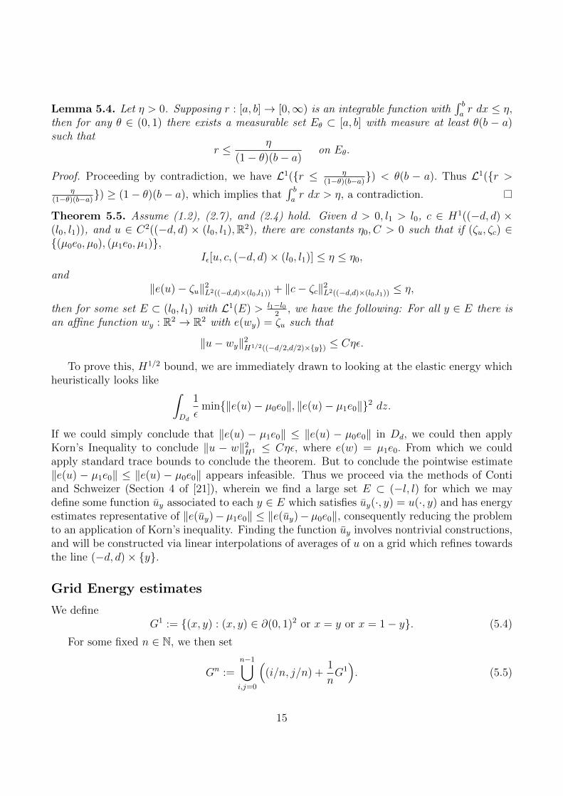
We defineG1 := (x, y) : (x, y) ∈ ∂(0, 1)2 or x = y or x = 1− y. (5.4)

For some fixed n ∈ N, we then set

Gn :=n−1⋃i,j=0

((i/n, j/n) +

1

nG1). (5.5)

15

Figure 1: G1, see (5.4). Figure 2: G2, see (5.5).

For some fixed k ∈ N, we define dk := 2−k and suppose z = (x, y), z′ = (x′, y′) ∈ R2 (withy < y′) are the left vertices of a parallelogram P with a base of length dk parallel to the x-axis;consider the affine map Lk(z, z

′) : R2 → R2 which maps (0, 1)2 onto P with Lk(z, z′)(0, 0) = z

and Lk(z, z′)(0, 1) = z′.

We define

Gnk(z, z′) := Lk(z, z

′)[∆2k−1⋃

i=0

((i, 0) +Gn)], (5.6)

where ∆ > 0 is such that ∆2k is an integer.

Figure 3: G12(z, z′) for ∆ = 1, z = (0, 0), z′ = (1/4, 1), see (5.6).

Let

gε(x, y) :=1

εf(c(x, y)) + ε‖∇c(x, y)‖2 +

1

ε‖e(u(x, y))− c(x, y)e0‖2. (5.7)

Up to modification of a few constants, the proof of the following theorem follows closely the oneof Lemma 4.3 in [21], and hence we refer the reader to this for a proof.

Theorem 5.6. Assume (1.2), (2.7), and (2.4) hold. Given θ ∈ (0, 1), δ ∈ (0, 1/4), d > 0,l1 > l0, and (ζu, ζc) ∈ (µ0e0, µ0), (µ1e0, µ1), there are constants η0, ε0, C, k0,∆, Cd,l > 0 suchthat for all ε ∈ (0, ε0), u ∈ C2((−d, d)× (l0, l1),R2), c ∈ C1((−d, d)× (l0, l1), [0, 1]) satisfying

Iε[u, c, (−d, d)× (l0, l1)] ≤ η ≤ η0

16

and‖e(u)− ζu‖2

L2((−d,d)×(l0,l1)) + ‖c− ζc‖2L2((−d,d)×(l0,l1)) ≤ η,

we may find a set E ⊂ (l0, l1) with L1(E) > l1−l02

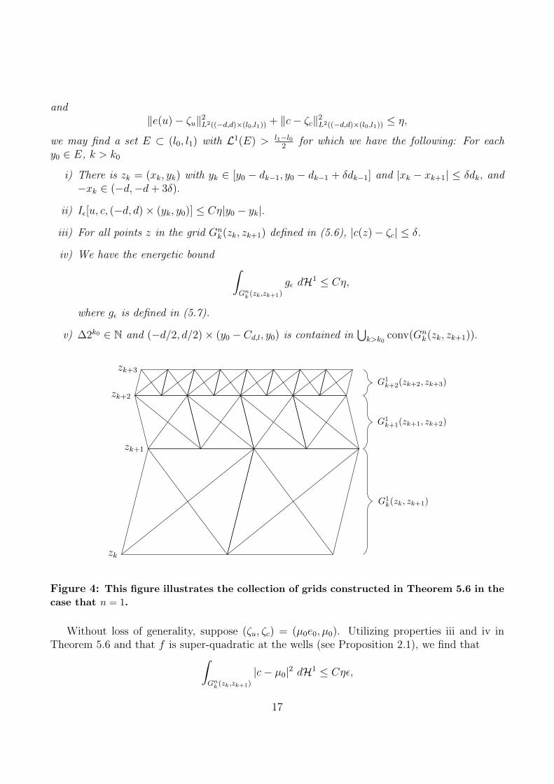
for which we have the following: For eachy0 ∈ E, k > k0

i) There is zk = (xk, yk) with yk ∈ [y0 − dk−1, y0 − dk−1 + δdk−1] and |xk − xk+1| ≤ δdk, and−xk ∈ (−d,−d+ 3δ).

ii) Iε[u, c, (−d, d)× (yk, y0)] ≤ Cη|y0 − yk|.

iii) For all points z in the grid Gnk(zk, zk+1) defined in (5.6), |c(z)− ζc| ≤ δ.

iv) We have the energetic bound ∫Gnk (zk,zk+1)

gε dH1 ≤ Cη,

where gε is defined in (5.7).

v) ∆2k0 ∈ N and (−d/2, d/2)× (y0 − Cd,l, y0) is contained in⋃k>k0

conv(Gnk(zk, zk+1)).

zk

G1k(zk, zk+1)

zk+1

G1k+1(zk+1, zk+2)

zk+2

zk+3

G1k+2(zk+2, zk+3)

Figure 4: This figure illustrates the collection of grids constructed in Theorem 5.6 in the

case that n = 1.

Without loss of generality, suppose (ζu, ζc) = (µ0e0, µ0). Utilizing properties iii and iv inTheorem 5.6 and that f is super-quadratic at the wells (see Proposition 2.1), we find that∫

Gnk (zk,zk+1)

|c− µ0|2 dH1 ≤ Cηε,

17

which by Minkowski’s inequality (see [28]) and property iv in Theorem 5.6 allows us to furtherconclude ∫

Gnk (zk,zk+1)

‖e(u)− µ0e0‖2 dH1 ≤ Cηε. (5.8)

We include a lemma of Conti and Schweizer [21] relating energy bounds on one element ofthe grid to an affine approximation of the function u. Let

L :=

[1/l s0 l

](5.9)

be the matrix mapping the unit square onto the parallelogram with vertices (0, 0), (1/l, 0), (s, l),and (s+ 1/l, l). For all s, l with |s|+ |l− 1| sufficiently small, the parallelogram is “close” to thesquare.

Letting a ∈ R2, s− := 0, s+ := s, l− := 0, and l+ := l, we define (see Figure 5) the segmentsγ±i on the grid given by a+ L(dGn) as

γ±i := a+(

(s±d+i

n(d/l), s±d+

i+ 1

n(d/l))× dl±

), (5.10)

with left endpoints z±i given by

z±i := a+ (s±d+i

n(d/l), dl±). (5.11)

Across all parallelograms sufficiently close to the square, we have the following affine approx-imation result:

Lemma 5.7. (Lemma 4.4, Remark 4.5 in [21]) Suppose a ∈ R2, d > 0, and ζu ∈ µ0e0, µ1e0.There exist constants δ, t0, C > 0 such that for all s, l, with

|s|+ |l − 1| < δ, (5.12)

and u ∈ H1(a+ L(0, d)2,R2), with

1

d2

∫a+L(0,d)2

min‖e(u)− µ0e0‖2, ‖e(u)− µ1e0‖2 dz ≤ σ

and1

d

∫a+L(dGn)

‖e(u)− ζu‖2 dH1 ≤ σ,

we may find φ ∈ R and w0 ∈ R2 such that for i = 0, . . . , n− 1,

u±i := −∫γ±i

u dH1

andw±i := w0 + ζu(z

±i ) +Rφ(z±i ),

we have‖u±i − w±i ‖2 ≤ Cσd2.

We recall that Rφ, Gn, and L are defined in (2.1), (5.5), and (5.9) respectively. Furthermore,γ±i and z±i are depicted in Figure 5.

18

γ−0

•z−2

γ+1

•z+3

Figure 5: Grid L(dG4) with segments γ±i , see (5.10), and points z±i , see (5.11).

To obtain the H1/2 bound in Theorem 5.5, it is essential that we estimate how φ changesbetween neighboring parallelograms. We collect these estimates in the following lemma.

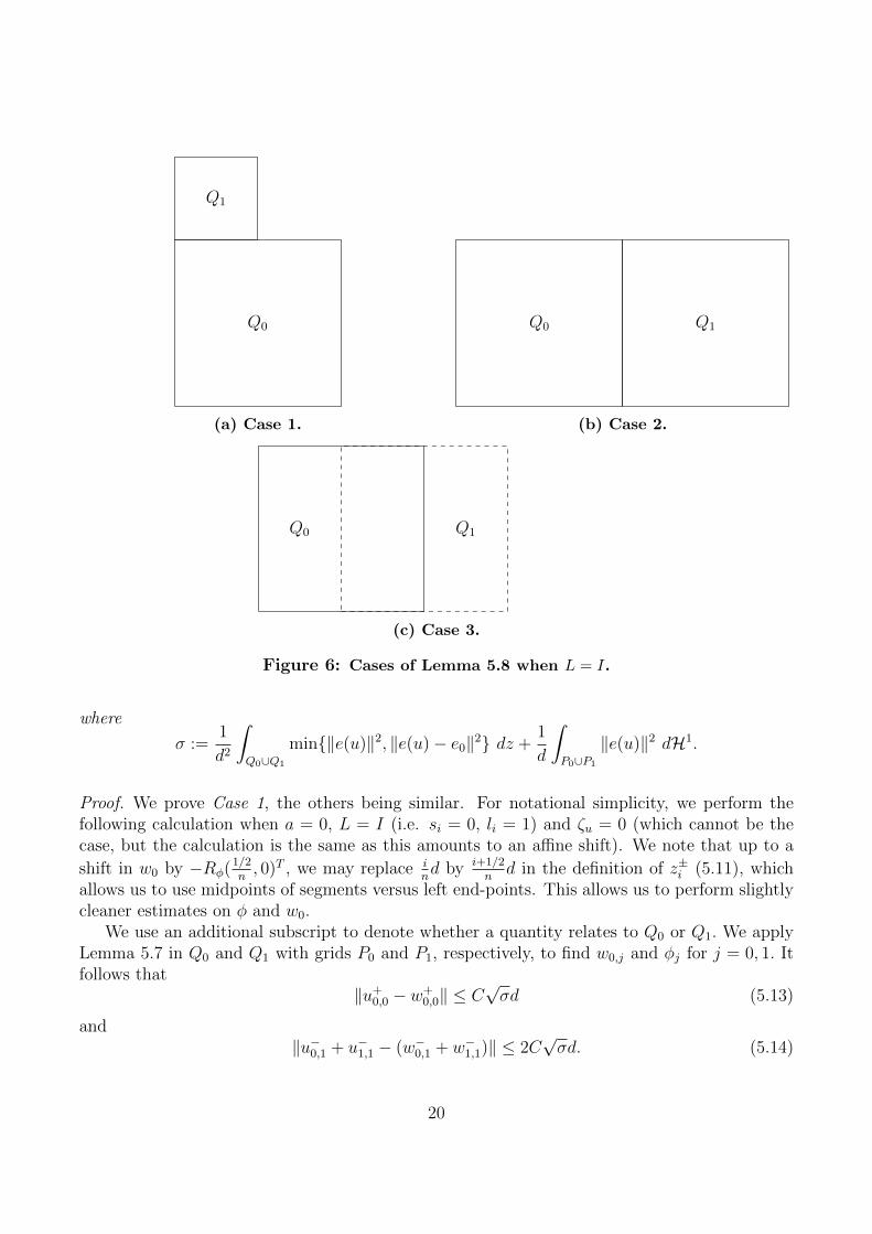
Lemma 5.8. Suppose n = 4, a ∈ R2, Q0 = L0[a+ (0, d)2], and one of the following casesCase 1: Q1 = L1[a+ (0, d) + (0, 1

2d)× (0, 1

2d)],

Case 2: Q1 = L0[a+ (d, 0) + (0, d)× (0, d)],Case 3: Q1 = L0[a+ (1

2d, 0) + (0, d)× (0, d)],

where L0 and L1 are affine maps with linear part of the form (5.9) with parameters li, si,subindexed by 0 and 1 respectively, satisfying condition (5.12) of Lemma 5.7. We further assumethat L0(0, d) = L1(0, d) and L0(d, d) = L1(d, d). Then if u ∈ H1((Q0 ∪Q1)o,R2), we have thatparameters φ0 and w0,0 associated to the grid P0 = L0(a + dG4) and parameters φ1 and w0,1

associated to the gridCase 1: P1 = L1(a+ (0, d) + 1

2dG4),

Case 2: P1 = L0(a+ (d, 0) + dG4),Case 3: P1 = L0(a+ (0, 1

2d) + dG4),

by applications of Lemma 5.7 satisfy the bounds

‖w0,0 − w0,1‖ ≤ C√σd

and|φ0 − φ1‖ ≤ C

√σ,

19

Q0

Q1

(a) Case 1.

Q0 Q1

(b) Case 2.

Q0 Q1

(c) Case 3.

Figure 6: Cases of Lemma 5.8 when L = I.

where

σ :=1

d2

∫Q0∪Q1

min‖e(u)‖2, ‖e(u)− e0‖2 dz +1

d

∫P0∪P1

‖e(u)‖2 dH1.

Proof. We prove Case 1, the others being similar. For notational simplicity, we perform thefollowing calculation when a = 0, L = I (i.e. si = 0, li = 1) and ζu = 0 (which cannot be thecase, but the calculation is the same as this amounts to an affine shift). We note that up to a

shift in w0 by −Rφ(1/2n, 0)T , we may replace i

nd by i+1/2

nd in the definition of z±i (5.11), which

allows us to use midpoints of segments versus left end-points. This allows us to perform slightlycleaner estimates on φ and w0.

We use an additional subscript to denote whether a quantity relates to Q0 or Q1. We applyLemma 5.7 in Q0 and Q1 with grids P0 and P1, respectively, to find w0,j and φj for j = 0, 1. Itfollows that

‖u+0,0 − w+

0,0‖ ≤ C√σd (5.13)

and‖u−0,1 + u−1,1 − (w−0,1 + w−1,1)‖ ≤ 2C

√σd. (5.14)

20

Furthermore, as Q0 and Q1 overlap at their top and bottom boundary respectively, we have

u+0,0 =

1

2(u−0,1 + u−1,1). (5.15)

Consequently, using the definition of w±i,j, equation (5.15), the triangle inequality, followed byapplication of the bounds (5.13) and (5.14), we find

‖w0,0 − w0,1 +Rφ0−φ1((1/2)d/n, d)T‖ = ‖w+0,0 −

1

2(w−0,1 + w−1,1)‖ ≤ C

√σd.

By a similar argument, since u+1,0 = 1

2(u−2,1 + u−3,1), we find

‖w0,0 − w0,1 +Rφ0−φ1((3/2)d/n, d)T‖ ≤ C√σd.

We note that to obtain both of these estimates is where we needed n = 4. Taking the differenceof the terms, we find

(d/n)|φ0 − φ1| = ‖Rφ0−φ1(d/n, 0)T‖ ≤ C√σd,

which implies |φ0 − φ1| ≤ C√σ. From this, it also follows that ‖w0,0 − w0,1‖ ≤ C

√σd.

With this in hand, we have enough tools to prove Theorem 5.5.

Proof of Theorem 5.5. Given that the energy bounds of Lemma 5.7 and equation (5.8) are inde-pendent of c, we do not concern ourselves with the function. We assume that ζu = µ0e0. Shiftingu by the affine function −µ0e0(x, y)T , we can assume that one well is ζu = 0 and the other wellis e0.

Fix the grid parameter n = 4. Let ∪kG4k be the grid as constructed in Theorem 5.6 with

parameter δ > 0 for some y ∈ E. We write

G4k =

iend⋃i=1

Pi,k

where each parallelogram grid element Pi,k is a translation of Lk(zk, zk+1)G4 and Piend,k is therightmost grid element. Choosing δ sufficiently small, each Pi,k may be written as a translationof (1+O(δ))L(0, dk)

2, with |s|+ |l−1| = O(δ). Thus the results of Lemma 5.7 still apply, and wefind an associated pair (wi,k, φi,k) satisfying the estimates of the lemma on the slightly rescaledgrid Pi,k.

We now work to define our function uy. For each Pi,k, we let γi,k be the bottom left segmentof the grid (in Lemma 5.7 this would be on the interval (0, d/n) × 0). We denote the lineaverage associated to this segment by

ui,k := −∫γi,k

u dH1. (5.16)

21

Note, for the last index iend for a fixed level k, we define uiend+1,k to be the line average over thebottom right segment for the rightmost grid element Piend,k.

For each i, k, we let zi,k be the bottom left vertex of Pi,k (ziend+1,k being the bottom right ofthe rightmost grid element). As such, we may divide Pi,k into two parallelograms P−i,k and P+

i,k,which each have a base of length dk/2 = dk+1, and have the vertex z2i+1,k+1 in common.

z1,k•

P−1,k P+1,k

γ1,k

z2,k z3,k• •

P−2,k P+2,k

γ2,k γ3,k

G4k(z1,k, z1,k+1) level

z1,k+1

z1,k+2

•

•

P1,k+1 P2,k+1 P3,k+1 P4,k+1 G4k+1(z1,k+1, z1,k+2) level

Figure 7: Geometric quantities involved in the proof of Theorem 5.5.

We define uy on conv(Pi,k) as follows:

• Along the lower boundary,

uy(θzi,k + (1− θ)zi+1,k) := θui,k + (1− θ)ui+1,k, (5.17)

for θ ∈ [0, 1].

• Along the upper boundary,

uy(θz2i+l,k+1 + (1− θ)z2i+l+1,k+1) := θu2i+l,k+1 + (1− θ)u2i+l+1,k+1, (5.18)

for θ ∈ [0, 1], l = 0, 1, where l designates whether we are considering the first (left) orsecond (right) half of the upper boundary.

• Throughout the convex hull of Pi,k,

uy(θz + (1− θ)(z + (z2i,k+1 − zi,k))) := θuy(z) + (1− θ)uy(z + (z2i,k+1 − zi,k)), (5.19)

for all z on the lower boundary of Pi,k, θ ∈ [0, 1].

22

In words, we define uy on the vertices of conv(Pi,k) in terms of the associated averages of u. Thenwe use linear interpolation to define the values on the upper and lower boundaries of conv(Pi,k).Lastly, we interpolate between the lower and upper boundaries by moving in lines parallel tothe sides of conv(Pi,k).

Given this construction of uy, we now wish to show that in each parallelogram conv(Pi,k),∇uy is close to the skew symmetric matrix Rφi,k . We restrict our attention to grid elements whichare not the rightmost, a simpler case. We introduce the parallelogram grid P ′i,k = P+

i,k ∪ P−i+1,k

for which Lemma 5.7 applies (associated terms have apostrophe, i.e. φ′i,k). Define

ν1 := (1, 0) =zi+1,k − zi,k‖zi+1,k − zi,k‖

, ν2 :=z2i,k+1 − zi,k‖z2i,k+1 − zi,k‖

.

As ν1 and ν2 are linearly independent, we have

‖∇uy −Rφi,k‖L∞(conv(Pi,k)) ≤∥∥∥∥ ∂

∂ν1

uy −Rφi,k(ν1)

∥∥∥∥L∞(conv(Pi,k))

+

∥∥∥∥ ∂

∂ν2

uy −Rφi,k(ν2)

∥∥∥∥L∞(conv(Pi,k))

.

(5.20)

As uy is constructed via linear interpolations (5.17), (5.18), (5.19), we bound ‖ ∂∂ν1uy−Rφi,k(ν1)‖L∞(conv(P−i,k))

via difference quotients along the top and bottom boundary of P−i,k:∥∥∥∥ ∂

∂ν1

uy −Rφi,k(ν1)

∥∥∥∥L∞(conv(P−i,k))

≤C

(∥∥∥∥∥(uy −Rφi,k)(z′i,k)− (uy −Rφi,k)(zi,k)

‖z′i,k − zi,k‖

∥∥∥∥∥+

∥∥∥∥(uy −Rφi,k)(z2i+1,k+1)− (uy −Rφi,k)(z2i,k+1)

‖z2i+1,k+1 − z2i,k+1‖

∥∥∥∥)=C

(∥∥∥∥ui+1,k − ui,kdk

−Rφi,k(1, 0)T∥∥∥∥

+

∥∥∥∥u2i+1,k+1 − u2i,k+1

dk+1

−Rφi,k(1, 0)T∥∥∥∥) .

(5.21)

Similarly,∥∥∥∥ ∂

∂ν2

uy −Rφi,k(ν2)

∥∥∥∥L∞(conv(P−i,k))

≤C(∥∥∥∥ u2i,k+1 − ui,k‖z2i,k+1 − zi,k‖

−Rφi,k

(z2i,k+1 − zi,k‖z2i,k+1 − zi,k‖

)∥∥∥∥+

∥∥∥∥ u2i+1,k+1 − 12(ui,k + ui+1,k)

‖z2i+1,k+1 − 12(zi,k + zi+1,k)‖

−Rφi,k

(z2i+1,k+1 − 1

2(zi,k + zi+1,k)

‖z2i+1,k+1 − 12(zi,k + zi+1,k)‖

)∥∥∥∥)(5.22)

The bounds over P+i,k are once again similar and we do not state them.

23

We bound the horizontal finite difference along the lower boundary of Pi,k, which will accountfor both terms on the right hand side of (5.21) up to an application of Lemma 5.8. Define

σ′i,k := −∫

conv(Pi,k∪Pi+1,k)

min‖e(u)‖2, ‖e(u)− e0‖2 dz +1

dk

∫Pi,k∪Pi+1,k

‖e(u)‖2 dH1,

where the integral is performed over Pi+1,k versus P ′i,k for convenience, not necessity. We compute∥∥∥∥ui+1,k − ui,kdk

−Rφi,k(1, 0)T∥∥∥∥2

≤ 1

d2k

(‖ui+1,k − u′i,k −Rφi,k(dk/2, 0)T‖2 + ‖u′i,k − ui,k −Rφi,k(dk/2, 0)T‖2

)≤Cd2k

(‖ui+1,k − u′i,k −Rφ′i,k

(dk/2, 0)T‖2 + ‖Rφ′i,k−φi,k(dk/2, 0)T‖2

+ ‖u′i,k − wi,k −Rφi,k(z′i,k)‖2 + ‖ui,k − wi,k −Rφi,k(zi,k)‖2

)≤Cd2k

(‖ui+1,k − w′i,k −Rφ′i,k

(zi+1,k)‖2 + ‖u′i,k − w′i,k −Rφ′i,k(z′i,k)‖2

+ d2k|φ′i,k − φi,k|2 + Cσ′i,kd

2k

)≤C(σ′i,k + |φ′i,k − φi,k|2) ≤ Cσ′i,k,

(5.23)

where we have used thatz′i,k − zi,k = zi+1,k − z′i,k = (dk/2, 0)

and|φ′i,k − φi,k|2 ≤ Cσ′i,k, (5.24)

by Lemma 5.8, and

‖u′i,k − wi,k −Rφi,k(z′i,k)‖ ≤ C

√σ′i,kdk

along with

‖u′i,k − w′i,k −Rφ′i,k(z′i,k)‖ ≤ C

√σ′i,kdk,

which are consequences of Lemma 5.7 with ζu = 0 applied to Pi,k and P ′i,k, respectively (notethat in the notation of Lemma 5.7, u′i,k is u−2 associated with the grid Pi,k).

We define

σi,k :=−∫

conv(Pi,k)

min‖e(u)‖2, ‖e(u)− e0‖2+1

dk

∫Pi,k

‖e(u)‖2 dH1

+−∫

conv(P2i,k+1)

min‖e(u)‖2, ‖e(u)− e0‖2+1

dk+1

∫P2i,k+1

‖e(u)‖2 dH1

+−∫

conv(P2i+1,k+1)

min‖e(u)‖2, ‖e(u)− e0‖2+1

dk+1

∫P2i+1,k+1

‖e(u)‖2 dH1.

24

We note that ‖z2i,k+1− zi,k‖ = (1 +O(δ))dk by construction. Furthermore, up to translation, wehave that zi,k = 0, and ‖z2i,k+1‖ = (1 +O(δ))dk. Using Lemma 5.7 and Lemma 5.8, we computea finite difference in the direction of ν2 =

z2i,k+1−zi,k‖z2i,k+1−zi,k‖

on the left boundary of conv(Pi,k). This

estimate will be used to bound the first term of the right hand side of (5.22).∥∥∥∥ u2i,k+1 − ui,k‖z2i,k+1 − zi,k‖

−Rφi,k

(z2i,k+1 − zi,k‖z2i,k+1 − zi,k‖

)∥∥∥∥2

≤ C

‖z2i,k+1 − zi,k‖2

(‖u2i,k+1 − (w2i,k+1 +Rφ2i,k+1

(z2i,k+1))‖2 + ‖ui,k − (wi,k +Rφi,k(zi,k))‖2

+ ‖w2i,k+1 − wi,k‖2 + ‖Rφ2i,k+1−φi,k(z2i,k+1)‖2)≤ Cσi,k.

(5.25)Note that the integrals in the definition of σi,k associated with P2i+1,k+1 are not needed for theabove inequality, but will be necessary for the next bound.

We perform a similar calculation for near vertical finite differences along the common bound-ary of conv(P−i,k) and conv(P+

i,k). This estimate bounds the second term of the right hand side

of (5.22). Using that z2i+1,k+1 = 12(z2i,k+1 + z2i+2,k+1) and adding and subtracting the term

12(u2i,k+1 + u2i+2,k+1), we estimate∥∥∥∥ u2i+1,k+1 − 1

2(ui,k + ui+1,k)

‖z2i+1,k+1 − 12(zi,k + zi+1,k)‖

−Rφi,k

(z2i+1,k+1 − 1

2(zi,k + zi+1,k)

‖z2i+1,k+1 − 12(zi,k + zi+1,k)‖

)∥∥∥∥2

≤Cd2k

(1

4‖u2i,k+1 − ui,k −Rφi,k(z2i,k+1 − zi,k)‖2 +

1

4‖u2i+2,k+1 − ui+1,k −Rφi,k(z2i+2,k+1 − zi+1,k)‖2

+

∥∥∥∥1

2(u2i+2,k+1 + u2i,k+1)− u2i+1,k+1

∥∥∥∥2)≤C(σi,k + σi+1,k +

1

d2k

∥∥∥∥1

2(u2i+2,k+1 + u2i,k+1)− u2i+1,k+1

∥∥∥∥2)≤C(σi,k + σi+1,k + σ′2i,k+1 + σ′2i+2,k+1),

(5.26)where in the second inequality we have applied the analysis of finite differences along the leftboundaries and the bound |φi+1,k − φi,k|2 ≤ Cσ′i,k provided by Lemma 5.8. To see the lastinequality, we note∥∥∥∥1

2(u2i+2,k+1 + u2i,k+1)− u2i+1,k+1

∥∥∥∥≤‖u2i+2,k+1 − u2i+1,k+1 −Rφ2i+1,k+1

(dk+1, 0)T‖+ ‖u2i+1,k+1 − u2i,k+1 −Rφ2i+1,k+1(dk+1, 0)T‖,

which are the horizontal finite differences, modulo a term like (5.24) for the second term, whichhave already been analyzed, thus concluding the bound.

We defineRφ :=

∑i,k

χconv(Pi,k)Rφi,k ,

25

noting that by (2.1), (Rφ)sym = 0 almost everywhere. Let G :=⋃k conv(Gn

k). Applying (5.20),(5.21), (5.22), and the subsequent finite difference estimates (5.23), (5.25), (5.26), we have

‖∇uy−Rφ‖2L2(G)

≤C∑i,k

L2(conv(Pi,k))

(∥∥∥∥ui+1,k − ui,kdk

−Rφi,k(1, 0)T∥∥∥∥2

+

∥∥∥∥ u2i,k+1 − ui,k‖z2i,k+1 − zi,k‖

−Rφi,k

(z2i,k+1 − zi,k‖z2i,k+1 − zi,k‖

)∥∥∥∥2

+

∥∥∥∥u2i+1,k+1 − 12(ui,k + ui+1,k)

‖z2i,k+1 − zi,k‖−Rφi,k

(z2i+1,k+1 − 1

2(zi,k + zi+1,k)

‖z2i+1,k+1 − 12(zi,k + zi+1,k)‖

)∥∥∥∥2)≤C

∑i,k

L2(conv(Pi,k))(σi,k + σi+1,k + σ′2i,k+1 + σ′2i+2,k+1)

≤C∑i,k

L2(conv(Pi,k))

(−∫

conv(Pi,k)

min‖e(u)‖, ‖e(u)− e0‖2 +1

dk

∫Pi,k

‖e(u)‖2 dH1

)≤∫G

min‖e(u)‖2, ‖e(u)− e0‖2 dz +∑k

dk∑i

∫Pi,k

‖e(u)‖2 dH1

≤Cηε+ (∑k

dk)

∫Gnk

‖e(u)‖2 dH1 ≤ Cηε,

where in the last line we have applied the energy bounds from Theorem 5.6, and the bound in thesecond to last line follows by undoing the affine shift of u and using Iε[u, c, (−d, d)× (l0, l1)] ≤ ηin conjunction with f being a super-quadratic well. As (−d/2, d/2)× (y−Cd,l, y) ⊂ G, we have

‖e(uy)‖2L2((−d/2,d/2)×(y−1/2,y)) ≤C‖∇uy −Rφ‖2

L2(G) ≤ Cηε.

Applying Korn’s inequality (see [42]), subsequently the trace theorem (see [37]), and notingby continuity that uy(·, y) = u(·, y), we conclude the proof.

Proof of Theorem 5.2. We construct the desired sequence by forming a transitional layer ofthickness εi on the upper and lower halves of the box. We treat the upper half; the lower half isanalogous. Let ψ : R→ [0, 1] be a smooth cutoff function with ψ(x) = 1 for x < 0 and ψ(x) = 0for x > 1. For some yi ∈ (l/2, 3l/4) to be determined, let ψi(x, y) := ψ((y − yi)/εi). We define

ci := ψici + (1− ψi)c. (5.27)

We must be more cautious in defining ui as previously noted.By Proposition 4.1,

lim infi→∞

Iεi [ui, ci, (−2d, 2d)× (−l/8, l/8)] ≥ 4dK(ey),

and therefore by (5.3),limi→∞

Iεi [ui, ci, (−2d, 2d)× (l/4, l)] = 0.

26

For computational simplicity, we perturb the hypotheses of the theorem to consider

ui → u =: uey(x, y)− Sey(x, y)T in H1(D2d,R2) (5.28)

andci → c =: cey in L2(D2d)

(see (1.10) and (5.2) for relevant definitions). Hence

ηi := ‖ci−c‖2L2 +‖ui−u‖2

H1 +L2(|ci−c| ≥ 1/2−µ0)+Iεi [ui, ci, (−2d, 2d)×(l/4, l)]→ 0. (5.29)

By Theorem 5.5 for each i sufficiently large, there is a set Ei ⊂ (l/2, 3l/4) such that L1(Ei) > l/8and for all y0 ∈ Ei there is an affine function

wy0(x, y) := (µ1e0 +Rφy0)(x, y)T + ay0 (5.30)

(depending on i) such that

‖ui − wy0‖2H1/2((−d,d)×y0) ≤ Cηiεi. (5.31)

Modifying a proof of Gagliardo’s (see Lemma 5.10 below this proof), we may constructvy0 ∈ H1((d/2, d/2)× (y0, l),R2) satisfying

vy0 = ui − wy0 on (−d/2, d/2)× y0vy0 = 0 on some neighborhood of (x, y) : y = l‖vy0‖2

H1((d/2,d/2)×(y0,l))≤ Cηiεi.

(5.32)

Defineui := ψiui + (1− ψi)(vi + wi), (5.33)

where vi = vyi , wi = wyi , and yi ∈ Ei is to be determined. We compute the energy for theconstructed sequence (recall (5.2)):

Iεi [ui, ci, Dd/2] =Iεi [ui, ci, D−d/2,εi

] +

∫Dd/2,εi

1

εif(ci) dz +

∫Dd/2,εi

εi‖∇ci‖2 dz

+

∫Dd/2,εi

1

εiC(e(ui)− cie0) : (e(ui)− cie0) dz +

∫D+d/2,εi

1

εiC(e(vi)) : e(vi) dz

=:A1 + A2 + A3 + A4 + A5.

We will bound terms A2, A3, A4, and A5 by ηi for appropriate choices of yi and explicitlycompute the limit of energy A1.Term A2: By (5.27),

A2 =

∫Dd/2,εi

1

εif(ψici + (1− ψi)c) dz

=

∫Dd/2,εi∩|ci−c|<1/2−µ0

1

εif(ψici + (1− ψi)c) dz

+

∫Dd/2,εi∩|ci−c|≥1/2−µ0

1

εif(ψici + (1− ψi)c) dz

=:A21 + A22.

(5.34)

27

To bound A22, we integrate yi over (l/2, 3l/4) and apply Fubini’s Theorem to find∫ 3l/4

l/2

1

εi

∫Dd/2,εi

χ|ci−c|≥1/2−µ0(x, y) d(x, y) dyi

=

∫ 3l/4

l/2

1

εi

∫ yi+εi

yi

∫ d/2

−d/2χ|ci−c|≥1/2−µ0(x, y) dx dy dyi

=1

εi

∫ εi

0

∫ 3l/4

l/2

∫ d/2

−d/2χ|ci−c|≥1/2−µ0(x, yi + y) dx dy dyi

≤∫ l

l/4

∫ d/2

−d/2χ|ci−c|≥1/2−µ0(x, t) dx dt ≤ ηi.

(5.35)

By Lemma 5.4, for θ ∈ (0, 1) there exists E1,θ ⊂ (l/2, 3l/4) with L1(E1,θ) > θl/4 such that

1

εi

∫Dd/2,εi

χ|ci−c|≥1/2−µ0(x, y) d(x, y) ≤ Cθηi

for all yi ∈ E1,θ. HenceA22 ≤ Cθ‖f‖∞ηi. (5.36)

To estimate A21, we use that f is decreasing on the interval [1/2, µ1] and increasing on [µ1, 1](see Proposition 2.1), and that in D2d,εi , we have c = µ1. Supposing ci ∈ [1/2, µ1], we findψici + (1− ψi)c ≥ ci ≥ 1/2, and consequently f(ψici + (1− ψi)c) ≤ f(ci), implying

A21 ≤∫Dd/2,ε

1

εif(ci) dz. (5.37)

Combining (5.36) and (5.37), we have

A2 ≤ Cθηi. (5.38)

Term A3: By (5.27), we have∫Ωεi

εi‖∇ci‖2 dz =

∫Ωεi

εi‖ψi∇ci + (ci − c)∇ψi‖2 dz

≤C∫

Ωεi

εi‖∇ci‖2 dz + C‖∇ψ‖∞1

εi

∫Ωεi

|ci − c|2 dz.

As in (5.35), by integrating in yi over (l/2, 3l/4) and applying Fubini’s Theorem and a change

28

of variables,∫ 3l/4

l/2

1

εi

∫Dd/2,εi

|ci(x, y)− c(x, y)| d(x, y) dyi

=

∫ 3l/4

l/2

1

εi

∫ yi+εi

yi

∫ d/2

−d/2|ci(x, y)− c(x, y)| dx dy dyi

=1

εi

∫ εi

0

∫ 3l/4

l/2

∫ d/2

−d/2|ci(x, yi + y)− c(x, yi + y)| dx dy dyi

≤∫ l

l/4

∫ d/2

−d/2|ci(x, t)− c(x, t)| dx dt ≤ Cηi.

(5.39)By Lemma 5.4, for θ ∈ (0, 1) there exists E2,θ ⊂ (l/2, 3l/4) with L1(E2,θ) > θl/4 such that

1

εi

∫Dd/2,εi

|ci − c| dz ≤ Cθηi

for all yi ∈ E2,θ. HenceA3 ≤ Cθηi. (5.40)

Term A4: We now estimate the elastic energy on the transition layer: By (5.27) and (5.33) wehave

A4 ≤C

εi

∫Dd/2,εi

‖ψi(e(ui)− cie0) + (1− ψi)(e(vi + wi)− ce0) + ((ui − wi − vi)⊗∇ψi)sym‖2 dz

≤Cεi

∫Dd/2,εi

(‖e(ui)− cie0‖2 + ‖∇vi‖2

)dz +

C

ε3i

∫Dd/2,εi

‖ui − wi − vi‖2 dz

=:A41 + A42, (5.41)

where we have used that in D2d,εi , c = µ1 by definition (1.10) and that e(wi) = µ1e0 by (5.30).By (1.2) and (5.32), A41 is controlled by Cηi. To bound A42, we utilize the Poincare inequalityin Dd/2,ε as ui − wi − vi = 0 on the lower boundary of this domain by (5.32) (see proof of thePoincare inequality in [37]). Explicitly,

A42 ≤C

εi

∫Dd/2,εi

‖∇(ui − wi − v)‖2 dz

≤Cεi

∫Dd/2,εi

‖∇ui − µ1e0‖2 + ‖φyi‖2 + ‖∇vi‖2 dz,

(5.42)

where in the last inequality we have used (2.1) and (5.30).Reasoning as in the proof of (5.35) and (5.39), we may apply Lemma 5.2 to find a set

E3,θ ⊂ (l/2, 3l/4) with L1(E3,θ) > θl/4 such that

C

εi

∫Dd/2,εi

‖∇ui − µ1e0‖2 dz ≤ Cθηi. (5.43)

29

The last term in the integrand on the right side of (5.42) is controlled by (5.32). Thus, itremains to control φi := φyi by ηi; to do this, we must first bound the constant ai := ayi in (5.30).Applying Lemma 5.4 to ‖ui− u‖2

L2(Dd/2,εi ), there is a set E4,θ ⊂ (l/2, 3l/4), with L1(E4,θ) > θl/4,

such that for all yi ∈ E4,θ ⊂ (l/2, 3l/4),∫ d/2

−d/2‖ui(x, yi)− µ1e0(x, yi)

T‖2 dH1 ≤ Cθηi,

where we have used (5.28). Consequently, supposing yi ∈ E0 ∩ E4,θ, we are able to compute

|a(2)i |2 ≤

∣∣∣∣∣−∫ d/2

−d/2ui(x, yi)− µ1e0(x, yi)

T )(2) dx

∣∣∣∣∣2

+

∣∣∣∣∣−∫ d/2

−d/2ui(x, yi)− wi(x, yi))(2) dx

∣∣∣∣∣2

≤Cηi + Cηiεi ≤ Cηi.

(5.44)

where we have used (2.1), (5.31), the fact that −∫ d/2−d/2 φix dx = 0, and the notation z = (z(1), z(2))

for a vector z ∈ R2. With this in hand, we may estimate

d3

12‖φi‖2 =

∫ d/2

−d/2‖φi‖2x2 dx ≤C

(|(ai)(2)|2 dx+

∫ d/2

−d/2|(ui(x, yi)− µ1e0(x, yi)

T )(2)|2 dx

+

∫ d/2

−d/2|(ui − wi)(2)|2 dx

)≤Cηi.

By a similar argument, one can conclude |(ai)(1)|2 ≤ Cηi too. Combining (5.42), (5.43), (5.44),and the previous inequalities, we conclude

C

ε3i

∫Dd/2,εi

‖ui − wi − vi‖2 ≤ Cηi.

By (5.41) this impliesA4 ≤ Cθηi. (5.45)

Term A5: By construction of vi (see (5.32)), we have that

A5 =

∫D+d/2,εi

1

εiC(e(vi)) : e(vi) dz ≤ C

∫D+d/2,εi

1

εi‖∇vi‖2 dz ≤ Cηi. (5.46)

Term A1: We may apply Proposition 4.1 and Theorem 4.4 to see

lim infi→∞

Iεi [ui, ci, D−d/2,εi

] ≥ lim infi→∞

Iεi [ui, ci, (−d/2, d/2)× (−l, l/4)]

≥dK(ey).

30

The upper bound follows by contradiction. Suppose that lim supi→∞

Iεi [ui, ci, D−d/2,εi

] > dK(ey). It

follows from Remark 4.2 and (4.3) that

4dK(ey) = limi→∞

Iεi [ui, ci, (−2d, 2d)× (−l, 3l/4)]

≥ lim infi→∞

Iεi [ui, ci, ((−2d,−d/2) ∪ (d/2, 2d))× (−l, 3l/4)]

+ lim supi→∞

Iεi [ui, ci, (−d/2, d/2)× (−l, 3l/4)]

>3dK(ey) + dK(ey) = 4dK(ey),

where in the second inequality we used Proposition 4.1 and horizontal translation. This contra-diction proves

limi→∞

Iεi [ui, ci, D−d/2,εi

] = dK(ey). (5.47)

Choosing θ sufficiently close to 1, by Lemma 5.9 below, we find that Ei ∩ (∩jEj,θ) 6= ∅, andthus there is yi such that all previous bounds are simultaneously satisfied. It follows that ui → uin H1(Dd/2,R2) (unknown till now as we needed estimates for ai and φi) and ci → c in L2(Dd/2).Utilizing energy bounds (5.38), (5.40), (5.45), (5.46), convergence of ηi (5.29), and convergenceof A1 (5.47), we find that

limi→∞

Iεi [ui, ci, Dd/2] = dK(ey),

concluding the theorem.

Lemma 5.9. Suppose Ei, i = 0, . . . , k, are measurable subsets of [0, 1], and λ ∈ (0, 1). Thenthere is ε0 = ε0(λ, k) such that if L1(E0) > λ and L1(Ei) > 1 − ε for some 0 < ε < ε0 for alli = 1, . . . , k, then

k⋂i=0

Ei 6= ∅. (5.48)

Proof. Using subadditivity, we have

L1(∩i>0Ei) = 1− L1(∪i>0ECi ) ≥ 1− kε.

Take ε0 < λ/k. If (5.48) does not hold,

L1(∩i≥0Ei) = L1(E0) + L1(∩i>0Ei) > λ+ (1− λ) = 1,

a contradiction.

Lemma 5.10. (see [37]) Given d, l > 0 and g ∈ H1/2((−d, d) × 0), we may construct v ∈H1((−d/2, d/2)× (0, l)) satisfying

v = g on (−d/2, d/2)× 0v = 0 on some neighborhood of (x, y) : y = l‖v‖2

H1((d/2,d/2)×(0,l)) ≤ C‖g‖H1/2((−d,d)×0),

for some constant C > 0 independent of g.

31

Proof. With an abuse of notation we treat g as a function of t ∈ (−d, d). Let η := mind, l > 0.Let φ ∈ C∞c ((−1, 1)) be a standard mollifier. For (x, y) ∈ (−d/2, d/2)× (0, η/2) we define

v(x, y) :=1

y

∫ d

−dφ((x− t)/y)g(t) dt.

Since φ is even,∫ d−d ∂φ((x− t)/y) dt = 0, so

∂v

∂x(x, y) =

1

(y)2

∫ d

−d∂φ((x− t)/y)g(t) dt

=1

(y)2

∫ d

−d∂φ((x− t)/y)[g(t)− g(x)] dt.

Consequently, ∣∣∣∂v∂x

(x, y)∣∣∣ ≤ C

(y)2

∫B(x,y)

|g(t)− g(x)| dt.

By Holder’s inequality and Fubini’s Theorem∫(−d/2,d/2)×(0,η/2)

∣∣∣∂v∂x

(x, y)∣∣∣2 d(x, y)

≤C∫

(−d/2,d/2)×(0,d/2)

1

(y)4

(∫B(x,y)

|g(t)− g(x)| dt)2

d(x, y)

≤C∫

(−d/2,d/2)×(0,d/2)

1

(y)3

∫B(x,y)

|g(t)− g(x)|2 dt d(x, y)

≤C∫

(−d/2,d/2)

∫(−d,d)

|g(t)− g(x)|2(∫ ∞|t−x|

1

(y)3dy)dt dx

=C

∫(−d/2,d/2)

∫(−d,d)

( |g(t)− g(x)||t− x|

)2

dt dx

≤C|g|H1/2((−d,d)×0).

Similarly, we compute

∂v

∂y(x, y) =

∫ d

−d

∂

∂y

(1

yφ((x− t)/y)

)g(t) dt

=

∫ d

−d

∂

∂y

(1

yφ((x− t)/y)

)[g(t)− g(x)] dt,

where in the last inequality we have used that for (x, y) ∈ (−d/2, d/2)× (0, η/2),

0 =∂

∂y(1) =

∂

∂y

(∫ d

−d

1

yφ((x− t)/y) dt

)=

∫ d

−d

∂

∂y

(1

yφ((x− t)/y)

)dt.

32

We bound ∣∣∣ ∂∂y

(1

yφ((x− t)/y)

)∣∣∣ =∣∣∣− 1

(y)2φ((x− t)/y) +

(x− t)(y)3

∂φ((x− t)/y)∣∣∣

≤ C

(y)2,

where we have used the fact that |x− t| ≤ y in the domain of integration. Thus we have∣∣∣∂v∂y

(x, y)∣∣∣ ≤ C

(y)2

∫B(x,y)

‖g(t)− g(x)‖ dt,

and we may proceed as before. We conclude that∫(−d/2,d/2)×(0,η/2)

∥∥∥∇v(z)∥∥∥2

dz ≤ C|g|H1/2((−d,d)×0).

Lastly, it remains to truncate the function, while preserving bounds. Let ψ : R → [0, 1] bea smooth function such that ψ(t) = χ(−∞,1/2](t) for all t 6∈ [1/4, 1]. For any α > 0, we definevα(x, y) := ψ(y/α)v(x, y). It is clear that∫

(−d/2,d/2)×(0,η/2)

∣∣∣ ∂∂xvα(z)

∣∣∣2 dz ≤ C|g|H1/2((−d,d)×0)

still holds.We compute∫

(−d/2,d/2)×(0,η/2)

∥∥∥ ∂∂yvα(z)

∥∥∥2

dz ≤C∫

(−d/2,d/2)×(0,η/2)

∥∥∥ ∂∂yv(z)

∥∥∥2

dz

+C

α2

∫(−d/2,d/2)×(0,η/2)

∣∣∣v(z)∣∣∣2 dz.

Using Fubini’s/Tonelli’s Theorem, it is straightforward to show that∫(−d/2,d/2)×(0,η/2)

∣∣∣v(z)∣∣∣2 dz ≤ C‖g‖2

L2(−d,d)×0. (5.49)

Consequently, for any α > 0, we have∫(−d/2,d/2)×(0,η/2)

∥∥∥∇vα(z)∥∥∥2

dz ≤ Cα‖g‖2H1/2((−d,d)×0).

Choosing α sufficiently small based on the geometry of the domain, we conclude the lemma bysetting v = vα. Note the desired L2 bound follows from inequality (5.49).

33

Proof of Step II

In this section, we use similar methods of proof as in the paper of Conti and Schweizer (Propo-sition 5.5 of [21]). We first prove a lemma relating energies to a geodesic distance similar to thatof the Modica-Mortola functional. In what follows, given a curve γ, we interchangeably use γas the set and parameterization representing the curve.

Lemma 5.11. Let gε be defined as in (5.7). For any δ > 0 there is h(δ) > 0 such that if γ isa C1-curve with length at least ε, range in (−d, d) × (−l, l), and

∫γgε dH1 ≤ h(δ), then either

|c(x, y)− µ1| ≤ δ or |c(x, y)− µ0| ≤ δ for all (x, y) ∈ γ.

Proof. Consider the geodesic distance between points on the interval I := [0, 1] defined by

dI(s, s′) := inf

∫ 1

0

√f(ψ(t))‖∇ψ(t)‖ dt : ψ ∈ C1(I, I), ψ(0) = s, ψ(1) = s′

. (5.50)

Leth0 := infdI(s, s′) : s, s′ ∈ I, |s− µ0| ≤ δ/2, |s′ − µ0| ≥ δ,

and similarly,h1 := infdI(s, s′) : s, s′ ∈ I, |s− µ1| ≤ δ/2, |s′ − µ1| ≥ δ.

Lastly, we define

h2 := inff(s) : x ∈ I, |s− µ1| ≥ δ/2, |s− µ0| ≥ δ/2.

Let h(δ) := 12

minh0, h1, h2.Assuming now that

∫γgε dH1 < h(δ) and H1(γ) > ε, we have

h2 >

∫γ

gε dH1 ≥ 1

εinff(c(x, y)) : (x, y) ∈ γH1(γ) ≥ inff(c(x, y)) : (x, y) ∈ γ,

which implies there must be a point (x, y) ∈ γ such that either |c(x, y)− µ1| ≤ δ/2 or |c(x, y)−µ0| ≤ δ/2. Without loss of generality, assume that the latter holds.

By (5.7), we compute

h0 >

∫γ

gε dH1 ≥∫γ

√f(c)‖∇c‖ dH1 ≥

∫ 1

0

√f(c γ)‖∇(c γ)‖ dt ≥ dI(c(x, y), c(x, y)),

where (x, y) ∈ γ and γ is a curve contained in γ connecting (x, y) and (x, y). By definition ofh0, this implies |c(x, y)− µ0| ≤ δ for all (x, y) ∈ γ as desired.

As in the proof of Proposition 4.1, via a diagonalization argument, for any domain (−d, d)×(−l, l), we may find sequences εi 0, ui → uey in H1((−d, d) × (−l, l),R2), and ci → cey inL2((−d, d)× (−l, l)) such that

limi→∞

Iεi [ui, ci, (−d, d)× (−l, l)] = 2dK(ey). (5.51)

However with respect to gamma convergence, the sequence εi is given a priori. Hence the criticalresult is the following:

34

Theorem 5.12. Assume (1.2), (2.7), and (2.4) hold. Let εi → 0, l > 0, and d > 0. There existsequences ui → uey and ci → cey such that

limi→∞

Iεi [ui, ci, (−d/2, d/2)× (−l, l)] = dK(ey). (5.52)

Proof. For notational convenience, we drop the subscript ey. Let εi 0, ui → u, and ci → c bethe sequences prior to the theorem statement for the domain (−4d, 4d)×(−l, l). By Theorem 5.2,we find sequences (not relabeled) ci ⊂ L2((−d, d)×(−l, l)) and ui ⊂ H1((−d, d)×(−l, l),R2)such that on the upper and lower boundaries of (−d, d) × (−l, l), ci = c and ui = u + χy>0wi,where wi is a skew affine function, with

limi→∞

Iεi [ui, ci, (−d, d)× (−l, l)] = 2dK(ey).

Thus we extend ci and ui to (−d, d)× R via constants or affine functions.For each i ∈ N, we let j(i) ∈ N be the smallest number such that j(i) > i and εj(i) < εi/i.

We then rescale our sequences as follows:

vi(x, y) :=εiεj(i)

ui

( εj(i)εi

(x, y)), bi(x, y) := ci

( εj(i)εi

(x, y)).

Letting αi := εiεj(i)

and using a change of variables, we find

Iεi [vi, bi, (−αid, αid)× R] = 2αidK(ey) + αiηj(i),

where ηi := Iεi [ui, ci, (−d, d)× (−l, l)]− 2dK(ey). Thus

bαic−1∑k=0

Iεi [vi, bi, (2k − bαic)d, (2(k + 1)− bαic)d)× R] =Iεi [vi, bi, (−bαicd, bαicd)× R]

≤2αidK(ey) + αiηj(i),

which implies there is some k0 ∈ −bαic,−bαic+ 2, . . . , bαic − 2 such that

Iεi [vi, bi, (k0d, (k0 + 2)d)× R] ≤ 2αibαic

dK(ey) +αibαic

ηj(i).

Translating the sequences, we assume k0 = −1. Taking the lim sup of the previous inequality,we find

lim supi→∞

Iεi [vi, bi, (−d, d)× R] ≤ 2dK(ey), (5.53)

as αibαic → 1. Note further that associated to each sequence vi, bi is some Li > 0 such that vi

is affine and bi is constant in each of the connected regions specified by the inequality |y| > Li.From this last fact, we are able to conclude that for each i ∈ N, Iεi [vi, bi, (−d, d)×R] ≥ Cd (see(5.59)).

35

We now work to truncate the domain under consideration from (−d, d)×R to (−d, d)×(−L,L)for some L > 0 such that

Cd ≤ lim infi→∞

Iεi [ui, ci, (−d, d)× (−L,L)] (5.54)

≤ lim supi→∞

Iεi [ui, ci, (−d, d)× (−L,L)] ≤ 2dK(ey),

where ui and ci are constructed from modifications of vi and bi and ui → u in H1((−d, d) ×(−L,L),R2), and ci → c in L2((−d, d)× (−L,L)).

In this direction, we let δ := (12− µ0)/2 and define the functions

f0(y) := L1(x ∈ (−d, d) : |bi(x, y)− µ0| ≤ δ) (5.55)

andf1(y) := L1(x ∈ (−d, d) : |bi(x, y)− µ1| ≤ δ). (5.56)

For large y, f0(y) = 0 and f1(y) = 2d. An analogous situation holds for y << 0. We utilize thesefunctions to isolate an interval where (5.54) will hold up to translation.

Note that the set of y satisfying f0(y) + f1(y) < 3d/2 has Lebesgue measure less thanC1εi ≤ C1. To see this, note that if f0(y) + f1(y) < 3d/2, then

L1(x ∈ (−d, d) : |bi(x, y)− µ1| > δ and |bi(x, y)− µ0| > δ) > d/2. (5.57)

This implies

d

2L1(y : inequality (5.57) holds)

≤∫RL1(x ∈ (−d, d) : |bi(x, y)− µ1| > δ and |bi(x, y)− µ0| > δ) dy

≤C∫

(−d,d)×Rf(bi) dz ≤ C1εi,

where we have used that f ≥ 0 with f(c) = 0 if and only if c = µ0 or c = µ1.We further note that the set on which both f0 > 0 and f1 > 0 is bounded in measure by a

constant C2. To see this, we use (5.7) to write

C1 ≥ Iεi [vi, bi, (−d, d)× R] =

∫R

∫(−d,d)

gεi(x, y) dx dy. (5.58)

By Lemma 5.11, if∫

(−d,d)gεi(x, y) dx ≤ h(δ), then either f0(y) or f1(y) is 0. Thus, we are

concerned in bounding

L1

(y ∈ R :

∫(−d,d)

gεi(x, y) dx > h(δ)

).

But by Markov’s Inequality and (5.58),

L1

(y ∈ R :

∫(−d,d)

gεi(x, y) dx > h(δ)

)≤ C1/h(δ).

36

ThusL1(y : f0(y) + f1(y) < 3d/2 ∪ y : f0(y) > 0, f1(y) > 0) ≤ C1 + C1/h(δ).

It follows that we may write R as the disjoint union of the three sets M , N , and O, where

• f0 = 0 and f1 > 3d/2 on M .

• f0 > 3d/2 and f1 = 0 on N .

• The remaining portion of R is O with L1(O) ≤ C1 + C1/h(δ).

Suppose y0 and y1 are such that f0(y0) > 3d/2 and f1(y1) > 3d/2. Then by (5.55) and (5.56),the set

E := x ∈ (−d, d) : |bi(x, y0)− µ0| ≤ δ ∩ x ∈ (−d, d) : |bi(x, y1)− µ1| ≤ δ

satisfiesL1(E) > d.

Assuming without loss of generality y0 < y1, we compute

Iεi [vi, bi, (−d, d)× (y0, y1)] ≥∫E

∫ y1

y0

gεi dy dx

≥ infdI(c, c′) : |c− µ0| ≤ δ, |c′ − µ1| ≤ δd = Cδd,

(5.59)

where dI is the geodesic distance from Lemma 5.11 (see (5.50)) and Cδ > 0.If we refer to an interval (y0, y1) as above as a transition, the energy bound (5.53) implies

there are at most J (independent of i) transitions.Note that (−∞,−Li) ⊂ N ⊂ (−∞, Li] by (5.55) and (5.56) and the comment following

these definitions. Hence we can define

y := infy : (y − ζ, y) ∩N = ∅ ≥ −Li > −∞,

where ζ > 2(C1 +C1/h(δ)) (the constant makes sure at most half the interval is in O). For someL > 0, we consider the interval (y − 2L, y − 2ζ), and divide the interval into segments of lengthζ (assuming 2L is divisible by ζ). Each interval intersects N by definition of y. If an intervalalso intersects M , it contains a transition. Thus for 2L > (J + 2)ζ, there must be at least onesuch interval, (z, z + ζ), which does not intersect M , as the number of transitions must be lessthan J . Consequently, in this interval, for at least half the y ∈ (z, z + ζ), f1(y) = 0. We notethis implies

ess infx∈(−d,d)

|bi(x, y)− µ1| ≥ δ (5.60)

for at least half the y ∈ (z, z + ζ). Similarly, we have

ess infx∈(−d,d)

|bi(x, y)− µ0| ≥ δ (5.61)

for at least half the y ∈ (y − ζ, y).

37

We consequently define

vi(x, y) := vi(x, y − L+ y), bi(x, y) := bi(x, y − L+ y),

for (x, y) ∈ (−d, d) × (−L,L) =: UL. By construction, there must be at least one transitionon the interval (−L,L), and consequently, these sequences satisfy (5.54). It remains to proveconvergence.

We defineηi := inf‖vi − u0‖H1(UL) + ‖bi − c0‖L2(UL) : (u0, c0) ∈ G,

where

G := (u0, c0) ∈ H1(UL,R2)× L2(UL) : u0(x, y) = u(x, y − a) + S(x, y)T + r,

c0(x, y) = c(x, y − a), for all (x, y) ∈ UL, and

a ∈ (−L+ ζ/2, L− ζ/2), S ∈ R2×2skew, r ∈ R2.

We claim ηi → 0. If not, there is a subsequence ηik bounded away from 0. Considering thecompactness Theorem 3.1, we have that vik → v in ∈ H1(UL,R2) and bik → b ∈ BV (UL, µ0, µ1)in L2(UL), with e(v) = be0. Without loss of generality, we may assume that bik → b pointwisea.e., and consequently, b satisfies (5.60) and (5.61). By Theorem 3.2, we have that v only hashorizontal or vertical interfaces. By the essential infimum estimates (5.60) and (5.61), there areno vertical interfaces. By the energy bounds (5.54), v can have at most one horizontal interfacetransition. Once again by the essential infimum estimates, b(x, y) = µ1 for y > L − ζ/2 andb(x, y) = µ0 for y < −L + ζ/2, else we contradict L2 convergence results. We conclude thatb = c(x, · − a) for some a ∈ (−L + ζ/2, L − ζ/2). It follows (v, b) ∈ G, which then contradictsthe assumption lim infk ηik > 0.

We conclude that ηi → 0. Translating functions and shifting by affine functions with skewgradient, we find ui : (−d, d)×(−ζ/2, ζ/2)→ R2 and ci : (−d, d)×(−ζ/2, ζ/2)→ [0, 1] satisfyingthe conclusion of the theorem with l = ζ/2. Applying Theorem 5.2, we obtain the theorem’sconclusion for l = ζ/2 where ui and ci are affine or constant (respectively) on the upper and lowerboundaries. Extending these functions to be affine or constant, the theorem’s conclusion holdson (−d/2, d/2)× R, which may then be truncated to the desired domain (−d/2, d/2)× (−l, l).

Proof of Step III

Proof of Theorem 5.1. Apply Theorem 5.12 to the domain (−2d, 2d) × (−l, l). Subsequently,apply Theorem 5.2 to conclude the result.

6 Limsup bound

We outline our plan to prove the lim sup bound on a strictly star-shaped Lipschitz domain Ω.In essence, we wish to put boxes around the interfaces, and interpolate between the sides ofthe boxes parallel to the interface by low energy sequences while maintaining regularity of thefunctions. More explicitly:

38

• Given u and c for which I0[u, c,Ω] is finite, we rescale the functions utilizing the fact thatthe domain is strictly star-shaped. This reduces the problem to the case of finitely manyinterfaces.

• Suppose without loss of generality that some interface has normal ey. Around this interface,we intersect the domain with a box of small width in the normal direction. For a givensequence εi, in each box, we use the characterization of the interfacial energy to constructa sequence of functions such that Iεi [ui, ci, (−d, d) × (−l, l)] → 2dK(ey), and both ui isaffine and ci is constant on the boundaries of the box parallel to the interface.

• We use the previous step to construct a low energy sequence which is equal to u plus a“small” skew affine function outside of the boxes and in the box is equal to the low energysequence with affine boundary conditions.

Theorem 6.1. (see also Proposition 5.1 of [21]) Assume (1.2), (2.7), and (2.4) hold. Supposeεi → 0 and that Ω is an open, strictly star-shaped domain with Lipschitz continuous boundary.For u ∈ H1(Ω;R2) and c ∈ BV (Ω; µ0, µ1) with I0[u, c,Ω] <∞, there are sequences ui →H1 uand ci →L2 c such that

lim supi→∞

Iεi [ui, ci,Ω] ≤ I0[u, c,Ω].

Proof. Assume without loss of generality that Ω is star-shaped about 0. Given θ ∈ (0, 1), werescale u and c to define

uθ(x, y) :=1

θu(θ(x, y)), cθ(x, y) := c(θ(x, y)), for (x, y) ∈ Ω.

We prove

lim supi→∞

Iεi [ui, ci,Ω] ≤ 1

θI0[u, c,Ω], (6.1)

for sequences ui → uθ in H1(Ω,R2) and ci → cθ in L2(Ω).Supposing we prove this for uθ and cθ, we may consider a sequence θk → 1 and find subse-

quences ui,ki and ci,ki such that satisfying inequality (6.1). Taking the lim sup with respectto k of the above inequality, we may apply a diagonalization argument to conclude the theorem.

Thus it remains to prove (6.1) for fixed θ. By Theorem 3.2, Jc = ∪jSj, where each Si is aconnected segment parallel to one of the axes. Thus Jcθ = ∪j(Ω ∩ 1

θSj) =: ∪jSj,θ. We note that

dist(Sj,θ, Sm,θ) > 0 for j 6= m as Sj and Sm can only intersect at endpoints, and thus the strictstar-shapedness implies, Sj,θ ∩ Sm,θ = ∅.

Furthermore, we have that Sj,θ = ∅ for all but finitely many of the j. Supposing not, wemay find a sequence zk such that zk ∈ Sjk ∩ θΩ for a strictly increasing sequence jkk. AsH1(Jc) <∞, H1(Sjk)→ 0. It follows that up to a subsequence zk → z0 ∈ ∂Ω. But by choice ofzk, we have z0 ∈ θΩ. This is a contradiction as ∂Ω ∩ θΩ = ∅ by strict star-shapedness.

From here on we only consider j for which Sj,θ is nonempty. Consider a horizontal segment,Sj = (x−j , x

+j )×yj. By strict star-shapedness 1

θ(x±j ×yj) 6∈ Ω. Thus we may find σ > 0 such

that 1θx±j × (1

θyj − σ, 1

θyj + σ)∩ Ω = ∅. We let Rj := (1

θx−j ,

1θx+j )× (1

θyj − σ, 1

θyj + σ). Similarly,

we define Rj for vertical interfaces. For σ sufficiently small, the sets Rj ∩ Ω are disjoint.

39

Associated to each Rj is unit normal νj and, as given by Theorem 5.1, there is a sequencewith uji , c

jii with uji = u+ χνj ·(x,y)>0(Rφji

(x, y)T + ai) and cji = c on the boundaries of the box

parallel to the interface and energy bounds as given by (5.52). We now seek to define sequencesui and ci.

We divide Ω\(∪jSj,θ) into connected components Ωk. We induce a partially ordered system(≺) on Ωk to make it into a downward directed set. Up to reordering, let Ω1 be a connectedcomponent with boundary only touching one interface. Ω1 is defined to be the minimal elementin the POS (≺). By star-shapedness, between every point of Ω1 and Ωk, there is a uniqueminimal sequence of connected components, Ωkini=1, k1 = 1 and kn = k, through which acontinuous path in Ω must travel to move between the points. We say Ωki ≺ Ωki+1

. Looking atall paths induces the desired POS (≺). Note, we have that each Ωk has a unique element Ωk′

which is the greatest element less than it. Letting Sj,θ be the interface separating the domainsΩk and Ωk′ . We define φki := φji and likewise for aji . Without loss of generality, we have that νjpoints from Ωk′ towards Ωk. Note we also treat (≺) as a partial order on k. With this, wedefine

ui(x, y) :=

uji (x, y) +

∑n≺k(Rφni

(x, y)T + ani ) (x, y) ∈ Rj ∩ Ω,Ωk ∩Rj 6= ∅,Ωk′ ∩Rj 6= ∅u(x, y) +

∑nk(Rφni

(x, y)T + ani ) not in the previous case, and (x, y) ∈ Ωk,

ci :=

cji (x, y) (x, y) ∈ Rj ∩ Ω,

c otherwise.

It follows that

lim supi→∞

Iεi [ui, ci,Ω] ≤∑j

lim supi→∞

Iεi [uji , c

ji , Rj]

≤1

θ

∑j

K(νi)H1(Si) ≤1

θI0[u, c,Ω],

proving the desired inequality (6.1). Convergence of the subsequences to uθ and cθ follows fromconvergence on the boxes and decay of φji and aji to 0 (see Theorem 5.2).

7 Mass Constraint

We now treat the case of Γ-convergence under the restriction of a mass constraint. Recall thatwe let mεε>0 ⊂ [0, 1] be a net converging to m0 ∈ [µ0, µ1] as ε → 0, and we wish to considerΓ-convergence restricting cε to satisfy −

∫Ωcε = mε. Obviously, the lim inf bound still holds, and

thus for given εi → 0, it remains to show that we may construct a sequence obtaining the limit.We write mi for mεi . We break this into cases depending on whether m0 = µ0, m0 = µ1, orm0 ∈ (µ0, µ1). In each case, we need to find some way to fluctuate the mass of the functionscε. To do this, we will emulate the proof of lim sup bound for the Modica-Mortola functional toconstruct a low energy perturbation of cε as previously constructed (see [36], [38]).

40

Proof of Theorem 1.2. Consider (u, c) such that I0[u, c,Ω] < ∞ and −∫

Ωc = m0. We construct

minimizing sequences for different cases.Case 1, m0 = µ0 or m0 = µ1: Without loss of generality, we treat the case that m0 = µ0.Note that in this case, the function c = µ0 and e(u) = µ0e0. Thus if mi = µ0, we may simplychoose ci = c. Consequently, in the following construction, we assume that mi 6= µ0 for all i.

We consider the energy functionals given by

Iεi [c′,Ω] := Iεi [u, c

′,Ω] =

∫Ω

1

ε

(f(c′) + ‖(c′ − µ0)e0‖2

)+ ε‖∇c′‖2 dz.

We condense notation by defining W (s) := f(s) + ‖(s − µ0)e0‖2. Note this is a single-wellpotential.

Subcase 1, µ0 < mi < µ1: We define the sequence Eηεz0>η>0 by Eη := B(z0, η)C , forany fixed z0 ∈ Ω such that B(z0, 2εz0) ⊂ Ω. Define Ei := Eηi = B(z0, ηi)

C , where ηi > 0 issuch that

µ0L2(Eηi ∩ Ω) + µ1L2(ECηi∩ Ω) = miL2(Ω). (7.1)

This assumes that mi is sufficiently close to µ0 (as given by some relation to εz0), whichwe do.

Define

φi(s) :=

∫ s

µ0

εi√εi +W (r)

dr.

Then, |φi(µ1)| ≤ ε1/2i . We note that φi is strictly increasing with differentiable inverse

φ−1i : [0, φi(µ1)]→ [µ0, µ1] satisfying

d

dtφ−1i (t) =

√εi +W (φ−1

i (t))

εi,

by the inverse function theorem. Extend φ−1i by constants at the boundary of [0, φi(µ1)].

We define

g0(t) :=

µ0, t ≤ 0,

µ1, t > 0,(7.2)

andvs(z) := φ−1

i (dEi(z) + s),

where

dEi(z) :=

−d(z, ∂Ei) if z ∈ Ei,d(z, ∂Ei) otherwise,

is the signed distance function of Ei (negative in Ei).We now wish to choose s such that the −

∫Ωvsi dz = mi. To do this, we apply the Mean

Value theorem to the function s 7→ −∫

Ωvs dz. We compute

−∫

Ω

φ−1i (dEi(z)) dz ≤−

∫Ω

g0(dEi(z)) dz = mi,

−∫

Ω

φ−1i (dEi(z) + φi(µ1)) dz ≥−

∫Ω

g0(dEi(z)) dz = mi.

41

Thus, for some si ∈ [0, φi(µ1)], we have −∫

Ωvsi dz = mi. Define ci := vsi . We now wish to

perform a precise estimate on ci. Since dEi is Lipschitz continuous and ‖∇dEi(z)‖ = 1 fora.e. z ∈ R2 \ ∂Ei, (see [27], [36], [10]) we can apply the coarea formula (see [27],[37]) toobtain

Iεi [ci,Ω] =

∫Ω

1

εiW (φ−1

i (dEi(z) + si)) + εi‖∇(φ−1i (dEi(z) + si))‖2

=

∫ ηi

−si

( 1

εiW (φ−1

i (r + si)) + εi|(φ−1i )′(r + si)|2

)H1(z ∈ Ω : dEi(z) = r) dr

≤ sup−si<t<ηi

H1(z ∈ Ω : dEi(z) = t)∫ ηi+si

0

1

εiW (φ−1

i (r)) + εi|(φ−1i )′(r)|2 dr

≤ sup−si<t<ηi

H1(z ∈ Ω : dEi(z) = t)∫ ηi+si

0

εi +W (φ−1i (r))

εi+ εi|(φ−1

i )′(r)|2 dr

= sup−si<t<ηi

H1(z ∈ Ω : dEi(z) = t)∫ ηi+si

0

2√εi +W (φ−1

i (r))|(φ−1i )′(r)| dr

≤ sup−si<t<ηi

H1(z ∈ R2 : dEi(z) = t)∫ 1

0

2√εi +W (s) ds

≤C(ε1/2i + ηi)

∫ 1

0

2√εi +W (s) ds→ 0

as i→∞. We now check convergence in L2(Ω) by the same means:∫Ω

|ci − µ0|2 =

∫Ω

|φ−1i (dEi(z) + si)− µ0|2

=

∫ ηi

−si|φ−1i (r + si)− µ0|2 H1(z ∈ Ω : dEi(z) = r) dr

≤(|si|+ |ηi|) sup−si<t<ηi

H1(z ∈ R2 : dEi(z) = t)→ 0

With this, we have proven Γ-convergence.Subcase 2, mi < µ0: The proof is predominantly the same as the previous subcase. Wecomment on the changes. To define ηi, consider µ0L2(Eη ∩ Ω) = mi in place of (7.1). Weuse 0 in place of µ1 in the definition of (7.2).

Case 2, m0 ∈ (µ0, µ1): In this case, we know that Jc 6= ∅, and further, there must bea point z0 ∈ Ω such that B(z0, 2εz0) ⊂ Ω and B(z0, 2εz0) ∩ Jc = ∅. Thus by the construc-tion in Theorem 6.1, we can find a low energy sequence (ui, ci)i converging to (u, c) suchthat ci|B(z0,εz0 )e0 = e(u)|B(z0,εz0 ) = µ0e0 for all i. Likewise, we can find z1 ∈ ∂Ω such thatci|B(z1,εz1 )e0 = e(u)|B(z1,εz1 ) = µ1e0 with B(z1, 2εz1) ⊂ Ω and B(z1, 2εz1) ∩ Jc = ∅.

We note that mi → m0, and −∫

Ωci dz → m0. Supposing −

∫Ωci dz < mi, we perform the same

procedure from the preceding section on B(z0, εz0) to construct cφ,i : B(z0, εz0) ∩ Ω → [0, 1](utilizing Eη = B(z0, η)C) with mass

−∫B(z0,εz0 )

cφ,i dz =miL2(Ω)−

∫Ωci dz

L2(B(z0, εz0))+ µ0,

42

(which makes sense for sufficiently large i) and

limiIεi [cφ,i, ui, B(z0, εz0)] = 0.

We define

ci(z) :=

ci if z ∈ Ω \B(z0, εz0),

cφ,i if z ∈ Ω ∩B(z0, εz0),

which satisfies ci → c in L2(Ω) and is directly shown to satisfy −∫

Ωci dz = mi.

We note by Theorem 4.4 the sequence (ui, ci) is of minimal energy on every Lipschitz subsetof Ω, and it follows Iεi [ui, ci, B(z0, εz0) ∩ Ω]→ 0. Thus,

limi→∞

Iεi [ui, ci,Ω] = limi→∞

Iεi [ui, ci,Ω].

Similarly, if −∫

Ωci dz > mi, we would perform the analogous calculation about z1 to decrease

the mass of ci. Consequently, we have shown the desired Γ-convergence result.

Acknowledgments

This paper is part of the author’s Ph.D. thesis at Carnegie Mellon University under the directionof Irene Fonseca and Giovanni Leoni. The author is deeply indebted to these two for theirmany hours spent watching the author scribble at a board and for expert guidance on manymathematical topics. Furthermore, the author is thankful for their many suggestions as to theorganization of the paper and spotting a plethora of typos, which greatly improved the paper.The author was partially supported by National Science Foundation Grants DMS 1906238 andDMS 1714098.

References

[1] Press release: The Nobel Prize in Chemistry 2019, https://www.nobelprize.org/prizes/chemistry/2019/press-release/, Accessed: 2019-11-22.

[2] N. Acharya, Phase field modeling of electrodeposition process in lithium metal batteries, MSThesis at Missouri University of Science and Technology (2016).

[3] L. Ambrosio, Metric space valued functions of bounded variation, Annali della Scuola Nor-male Superiore di Pisa - Classe di Scienze Ser. 4, 17 (1990), no. 3, 439–478 (en).

[4] L. Ambrosio, N. Fusco, and D. Pallara, Functions of bounded variation and free discontinu-ity problems, Oxford Mathematical Monographs, The Clarendon Press, Oxford UniversityPress, New York, 2000.

[5] P. Bai, D. A. Cogswell, and M. Z. Bazant, Suppression of phase separation in LiFePO4

nanoparticles during battery discharge, Nano Letters 11 (2011), 4890–4896.

43

[6] J. M. Ball and R. D. James, Fine phase mixtures as minimizers of energy, Archive forRational Mechanics and Analysis 100 (1987), no. 1, 13–52.

[7] R. W. Balluffi, S. M. Allen, W. C. Carter, and R. A. Kemper, Kinetics of materials, JohnWiley & Sons, 2005.

[8] A. Barroso and I. Fonseca, Anisotropic singular perturbations—the vectorial case, Proceed-ings of the Royal Society of Edinburgh: Section A Mathematics 124 (1994), 527 – 571.

[9] M. Z. Bazant, Theory of chemical kinetics and charge transfer based on nonequilibriumthermodynamics, Accounts of chemical research 46 (2013).

[10] G. Bellettini, Lecture notes on mean curvature flow, barriers and singular perturbations,Scuola Normale Superiore Pisa, 2013.

[11] G. Bellettini, A. Chambolle, and M. Goldman, The Γ-limit for singularly perturbed func-tionals of perona–malik type in arbitrary dimension, Mathematical Models and Methods inApplied Sciences 24 (2013).

[12] K. Bhattacharya, Microstructure of martensite: Why it forms and how it gives rise to theshape-memory effect, Oxford University Press, 2003.

[13] D. Burch and M. Z. Bazant, Size-dependent spinodal and miscibility gaps for intercalationin nanoparticles, Nano letters 9 (2009), no. 11, 3795–3800.

[14] D. Burch, G. Singh, G. Ceder, and M. Z. Bazant, Phase-transformation wave dynamics inLiFePO4, Solid State Phenomena 139 (2008), 95–100.

[15] G. Caginalp, Phase field models and sharp interface limits: Some differences in subtlesituations, Rocky Mountain J. Math. 21 (1991), no. 2, 603–615.

[16] J. Cahn and J. Hilliard, Free energy of a nonuniform system. i. interfacial free energy, TheJournal of chemical physics 28 (1958), no. 2, 258–267.

[17] A. Chambolle, A. Giacomini, and M. Ponsiglione, Piecewise rigidity, Journal of FunctionalAnalysis, v.244, 134-153 (2007) 244 (2007).

[18] D. A. Cogswell and M. Z. Bazant, Coherency strain and the kinetics of phase separation inLiFePO4 nanoparticles, ACS nano 6 (2012), no. 3, 2215–2225.

[19] S. Conti, I. Fonseca, and G. Leoni, A gamma-convergence result for the two gradient theoryof phase transitions, Communications on Pure and Applied Mathematics 55 (2001).

[20] S. Conti and B. Schweizer, Rigidity and gamma convergence for solid-solid phase transitionswith so(2) invariance, Communications on Pure and Applied Mathematics 59 (2006), 830– 868.

44

[21] , A sharp-interface limit for a two-well problem in geometrically linear elasticity,Archive for Rational Mechanics and Analysis 179 (2006), 413–452.

[22] H. Dal and C. Miehe, Computational electro-chemo-mechanics of lithium-ion battery elec-trodes at finite strains, Computational Mechanics 55 (2015), no. 2, 303–325.

[23] E. Davoli and M. Friedrich, Two-well rigidity and multidimensional sharp-interface limitsfor solid-solid phase transitions, 2018.

[24] C. De Lellis and F. Otto, Structure of entropy solutions to the eikonal equation, Journal ofthe European Mathematical Society 5 (2003), no. 2, 107–145.

[25] A. DeSimone, S. Muller, R. V. Kohn, and F. Otto, A compactness result in the gradienttheory of phase transitions, Proceedings of the Royal Society of Edinburgh: Section AMathematics 131 (2001), no. 4, 833–844.

[26] G. Dolzmann and S. Muller, Microstructures with finite surface energy: the two-well prob-lem, Archive for Rational Mechanics and Analysis 132 (1995), no. 2, 101–141.

[27] L. Evans and R. Gariepy, Measure theory and fine properties of functions, Studies in Ad-vanced Mathematics, CRC Press, Boca Raton, FL, 1992.

[28] I. Fonseca and G. Leoni, Modern methods in the calculus of variations: Lp spaces, SpringerScience & Business Media, 2007.

[29] I. Fonseca and C. Mantegazza, Second order singular perturbation models for phase transi-tions, Siam Journal on Mathematical Analysis 31 (2000).

[30] I. Fonseca and S. Muller, Relaxation of quasiconvex functional in BV (Ω,Rp) for integrandsf(x, u,∇u), Archive for Rational Mechanics and Analysis 123 (1993), no. 1, 1–49.

[31] I. Fonseca and L. Tartar, The gradient theory of phase transitions for systems with twopotential wells, Proceedings of the Royal Society of Edinburgh: Section A Mathematics111 (1989), no. 1-2, 89–102.

[32] E. De Giorgi, Sulla convergenza di alcune successioni d’integrali del tipo dell’area, Rend.Mat. IV (1975), no. 8.

[33] B. C. Han, A. Van der Ven, D. Morgan, and G. Ceder, Electrochemical modeling of inter-calation processes with phase field models, Electrochimica Acta 49 (2004), no. 26, 4691 –4699.

[34] R. V. Kohn and S. Muller, Surface energy and microstructure in coherent phase transitions,Communications on Pure and Applied Mathematics 47 (1994), 405 – 435.

[35] G. Lauteri and S. Luckhaus, Geometric rigidity estimates for incompatible fields in dimen-sion ≥ 3, 2017.

45

[36] G. Leoni, Gamma convergence and applications to phase transitions, summer school, May2013.

[37] G. Leoni, A first course in Sobolev spaces, 2 ed., Graduate Studies in Mathematics, vol.181, American Mathematical Society, Providence, RI, 2017.

[38] L. Modica and S. Mortola, Un esempio di Γ-convergenza, Boll. Un. Mat. Ital. B (5) 14(1977), no. 1, 285–299.

[39] S. Muller, Variational models for microstructure and phase transitions, pp. 85–210, SpringerBerlin Heidelberg, Berlin, Heidelberg, 1999.

[40] S. Muller, L. Scardia, and C. Zeppieri, Geometric rigidity for incompatible fields and anapplication to strain-gradient plasticity, Indiana University Mathematics Journal 63 (2014),no. 5, 1365–1396 (English).

[41] E. B. Nauman and D. Q. He, Nonlinear diffusion and phase separation, Chemical Eng. Sci.(2001), no. 6, 1999–2018.

[42] J. A. Nitsche, On korn’s second inequality, ESAIM: Mathematical Modelling and NumericalAnalysis - Modelisation Mathematique et Analyse Numerique 15 (1981), no. 3, 237–248(en).

[43] G. K. Singh, G. Ceder, and M. Z. Bazant, Intercalation dynamics in rechargeable batterymaterials: general theory and phase-transformation waves in LiFePO4, Electrochimica Acta53 (2008), no. 26, 7599–7613.

[44] Y. Zeng and M. Z. Bazant, Phase separation dynamics in isotropic ion-intercalation parti-cles, SIAM Journal on Applied Mathematics 74 (2013).

46