Math 711 Homework

Austin Mohr

June 16, 2012

Problem 1

Proposition 1. Convergence in probability of a sequence of random variablesdoes not imply almost sure convergence of the sequence.

Proof. Let ([0, 1],B([0, 1]), λ) be the ambient probability space. Consider aprocess wherein, at the nth stage, we choose (independently at random) a closedsubinteral Fn of [0, 1] of length 1

n .

Define now the random variable Xn = I(Fn). Evidently, Xpr−→ 0, since, for

each n, Xn is nonzero only on the interval of length 1n . Thus, for any ε > 0,

P (|Xn| > ε) =1

n→ 0.

To see that Xn does not enjoy almost sure convergence to zero, observe that,for each ω ∈ [0, 1],

∞∑n=1

P (Xn(ω) 6= 0) =

∞∑n=1

1

n

=∞.

Thus, by the Borel Zero-One Law, P (Xn(ω) 6= 0 i.o.) = 1, and so it cannot bethat Xn converges almost surely to zero.

Problem 2

Proposition 2. For any sequence Xn of random variables, there exists asequence of constants an such that Xn

anconverges almost surely to zero.

Proof. Let ε > 0 be given. Choose an such that P (|Xn| > ε) ≤ 12n . Observe

that

∞∑n=1

P (|Xn| > ε) ≤∞∑n=1

1

2n

<∞,

1

and so the Borel-Cantelli Lemma gives that P ([|Xn| > ε] i.o.) = 0. That is,

Xna.s.−→ 0.

Problem 3

Proposition 3. For a monotone sequence of random variables, convergence inprobability implies almost sure convergence.

Proof. Let Xn be a monotone sequence of random variables with Xnpr−→ X. It

follows that, for all ε > 0,

0 = limn→∞

P (|Xn −X| > ε)

= limN→∞

P

⋃n≥N

[|Xn −X| > ε]

(by monotonicity of the Xn)

= P

(lim supn→∞

[|Xn −X| > ε]

)= P ([|Xn −X| > ε] i.o.).

Therefore, Xna.s.−→ X.

Problem 4

Proposition 4. Let Xn be a sequence of random variables and define, foreach n, Yn = XnI|Xn| ≤ an. There exists a sequence an of positive realnumbers such that PXn 6= Yn i.o. = 0.

Proof. For each n, choose an such that P (|Xn| > an) ≤ 12n . Thus,

∞∑n=1

P (Xn 6= Yn) =

∞∑n=1

P (|Xn| > an)

≤∞∑n=1

1

2n

<∞.

By the Borel-Cantelli Lemma, we conclude that P ([Xn 6= Yn] i.o.) = 0.

Problem 5

Proposition 5. Suppose n points are chosen randomly on the unit circle. De-fine the random variable Xn to be the arc length of the largest arc not containingany of the chosen points. In this case, Xn → 0 almost surely.

2

Proof. Let ε > 0 be given. We have that

P ([Xn > ε] i.o.) = P

(lim supn→∞

[Xn > ε]

)

= limN→∞

P

⋃n≥N

[Xn > ε]

= limn→∞

P (Xn > ε) (by monotonicity of the Xn).

We bound this last probability by breaking the unit circle into 4πε disjoint in-

tervals of length ε2 . Thus, P (Xn ≤ ε) is no larger than the probability of having

a point contained in a every interval. Thus,

P ([Xn > ε] i.o.) = limn→∞

P (Xn > ε)

≤ limn→∞

4π

ε

(2π − ε

2

2π

)n= 0,

and so Xna.s.−→ 0.

Problem 6

Proposition 6. If, for all a < b,

P[Xn < a i.o.] and [Xn > b i.o.] = 0,

then limn→∞Xn exists almost surely.

Proof. By taking complements, we have

P[Xn ≥ a] or [Xn ≤ b] = 1,

for all sufficiently large n. If it is the case that the former holds for all a,then limn→∞Xn = ∞ almost surely. Similarly, if the latter holds for all b,then limn→∞Xn = −∞ almost surely. Otherwise, there is some c so thatP (Xn ≤ b) = 1 for all b ≥ c and P (Xn ≤ b) = 0 for all b < c. By keeping b = cfixed and letting a ↑ b, we see that limn→∞Xn = c almost surely.

Problem 7

Proposition 7. If Xn → 0 in probability, then, for any α > 0,

|Xn|α

1 + |Xn|αpr−→ 0.

3

Proof. Let ε > 0 be given. Choose N such that

P (|Xn| > ε1α ) < ε,

for all n ≥ N . It follows that

P (|Xn|α > ε) < ε

for all n ≥ N . Now,|Xn|α

1 + |Xn|α≤ |Xn|.

Thus, for all n ≥ N ,

P

(|Xn|α

1 + |Xn|α> ε

)≤ P (|Xn|α > ε)

< ε,

and so |Xn|α1+|Xn|α

pr−→ 0.

Problem 8

Proposition 8. If, for some α > 0,

|Xn|α

1 + |Xn|αpr−→ 0,

then Xnpr−→ 0.

Proof. Let ε > 0 be given. Choose N such that

P

(|Xn|α

1 + |Xn|α> ε

)< ε

for all n ≥ N . Now, (|Xn|

1 + |Xn|

)α≤ |Xn|α

1 + |Xn|α.

Thus, for all n ≥ N ,

P

((|Xn|

1 + |Xn|

)α> ε

)≤ P

(|Xn|α

1 + |Xn|α

)< ε,

and so

P

(|Xn|

1 + |Xn|> ε

1α

)< ε,

from which it follows that Xnpr−→ 0.

4

Problem 9

Proposition 9. Let Xn be a collection of independent random variables with

PXn = n2 =1

n2and PXn = −1 = 1− 1

n2

for all n. In this case,∑ni=1Xi converges almost surely to −∞ as n→∞.

Proof. Observe first that, by definition of the Xn, P (Xn ∈ n2,−1) = 1. Thatis, except for a null set, Xn takes on only the values n2 or −1.

Now, we have

∞∑n=1

P (Xn = n2) =

∞∑n=1

1

n2

<∞,

and so P ([Xn = n2] i.o.) = 0 by the Borel-Cantelli Lemma.Similarly,

∞∑n=1

P (Xn = −1) =

∞∑n=1

1− 1

n2

=∞,

and so P ([Xn = −1] i.o.) = 1 by the Borel Zero-One Law (note here that werequire the independence of the Xn).

Thus, for almost all ω ∈ Ω, there exists Nω such that Xn(ω) = −1 for alln ≥ Nω. It follows that

limn→∞

Sn(ω) = limn→∞

n∑i=1

Xi(ω)

=

Nω∑i=1

Xi(ω) +∑i>Nω

Xi(ω)

≤Nω∑i=1

n2 +∑i>Nω

−1

= −∞,

and so Sna.s.−→ −∞.

Problem 1

Proposition 10. Let E(X2)

= 1 and E (|X|) ≥ a > 0. For 0 ≤ λ ≤ 1,

P|X| ≥ λa ≥ (1− λ)2a2.

5

Proof. Let A denote the set |X| ≥ λa. We have

E (|X|) = E (|X|1A) + E (|X|1Ac) .

Now, applying Holder’s inequality to the first term,

E (|X|1A) ≤√

E (X2)E (12A)

=√P (A).

We have also that

E (|X|1Ac) < λa.

Taken together, we see that

a ≤ E (|X|)

≤√P (A) + λa.

Rearranging terms gives, √P (A) ≥ a− λa

= a(1− λ),

and so P (A) ≥ a2(1− λ)2, as desired.

Problem 2

Proposition 11. For 1 ≤ s ≤ t < ∞ and X ∈ Lt, ||X||s ≤ ||X||t (where

||X||p = (E (|X|p))1p ).

Proof. There is nothing to show for the case s = t, so we assume that s < t.Let α = t

s and β = tt−s , so that 1

α + 1β = 1. By Holder’s inequality,

E (|X|s) = E (|X|s · 1)

≤ E (|X|sα)1α · E

(1β) 1β

= E (|X|sα)1α

= E(|X|t

) st .

Thus,

||X||s = E (|X|s)1s

≤(E(|X|t

) st

) 1s

= E(|X|t

) 1t

= ||X||t<∞,

as desired.

6

Problem 3

For a random variable X, define

||X||∞ = supM : P|X| > M > 0

and alsoL∞ = X : ||X||∞ <∞.

Proposition 12. For X ∈ L∞ and 1 < p < q <∞,

0 ≤ ||X||1 ≤ ||X||p ≤ ||X||q ≤ ||X||∞.

Proof. Since X ∈ L∞, X is bounded, and so X ∈ Lt for any t. Thus, byProblem 2, it remains only to show that ||X||q ≤ ||X||∞. Now,

||X||q = (E (Xq))1q

≤ (Mq)1q (for some M > 0, since X ∈ L∞)

= M

= ||X||∞.

Proposition 13. For 1 < p < q <∞, L∞ ⊂ Lq ⊂ Lp ⊂ L1.

Proof. We show, equivalently, that X ∈ Lq implies X ∈ Lp whenever 1 ≤ p ≤q ≤ ∞. To that end, let 1 ≤ p ≤ q ≤ ∞ and let X ∈ Lq. Applying the previousresult, we have

||X||p ≤ ||X||q<∞,

and so X ∈ Lp.

Proposition 14. For X,Y ∈ L∞,

E (|XY |) ≤ ||X||1||Y ||∞.

Proof. Note first that, since L∞ ⊂ L1, X ∈ L1. Now,

E (|XY |) ≤ E (|XM |) (for some M > 0, since Y ∈ L∞)

= E (|X|) ·M= ||X||1||Y ||∞.

Proposition 15. For X,Y ∈ L∞,

||X + Y ||∞ ≤ ||X||∞ + ||Y ||∞.

7

Proof. It follows immediately that

||X + Y ||∞ = supM : P|X + Y | > M > 0≤ supM : P|X|+ |Y | > M > 0≤ supM : P|X| > M > 0+ supM : P|Y | > M > 0= ||X||∞ + ||Y ||∞.

Problem 4

Proposition 16. Let X ∈ L1, the map

χ : [1,∞]→ [0,∞]

defined according to χ(p) = ||X||p is continuous on [1, p0), where

p0 = supp ≥ 1 : ||X||p <∞.

Furthermore, the continuous function η(p) = log(||X||pp

)is convex on [1, p0).

Proof. For the continuity of χ, consider any sequence pn converging to p ∈[0, p0) and set ξ = |X|p+1. Note that ||ξ||p <∞. Since |X|pn → |X|p pointwiseand |X|pn ≤ ξ for all n, the Lebesgue dominated convergence theorem gives

E (Xpn)→ E (Xp) .

Since the operation of exponentiation is continuous, it follows that

(E (Xpn))1pn → (E (Xp))

1p .

That is, ||X||pn → ||X||p, and so χ is continuous in p.For the convexity of η, let u and v be arbitrary real numbers and let α ∈ [0, 1].

We seek to establish

log ||X||αu+αvαu+αv ≤ α log ||X||uu + α log ||X||vv,

where α = 1− α. By exponentiating both sides, it is equivalent to show

||X||αu+αvαu+αv ≤ ||X||αuu ||X||αvv .

It follows that via Holder’s inequality that

||X||αu+αvαu+αv = E(|X|αu+αv

)≤(E(

(|X|αu)1α

))α (E((|X|αv

) 1α

))α≤ (E (|X|u))

α(E (|X|v))α

= ||X||αuu ||X||αvv .

8

Problem 5

For random variables X and Y , define

ρ(X,Y ) = infδ > 0 : P|X − Y | ≥ δ ≤ δ.

In the space S of random variables, form the space E of equivalence classes[X] : X ∈ S where [X] = Y : X = Y a.s..

Proposition 17. The function ρ defined above is a metric on E. Moreover,

Xnpr−→ X if and only if ρ(Xn, X)→ 0.

Proof. We show first that ρ is well-defined on E. To that end, let X, X ′, Y , andY ′ be random variables with X = X ′ almost surely and Y = Y ′ almost surely.It follows that

ρ(X,Y ) = infδ > 0 : P|X − Y | ≥ δ ≤ δ= infδ > 0 : P|X ′ − Y ′| ≥ δ ≤ δ= ρ(X ′, Y ′).

By virtue of this, we will henceforth let a random variable X represent the entireequivalence class [X].

In what follows, let X, Y , and Z be random variables.We see immediately that

ρ(X,Y ) = infδ > 0 : P|X − Y | ≥ δ ≤ δ= 0

if and only if X = Y .We have next that

ρ(X,Y ) = infδ > 0 : P|X − Y | ≥ δ ≤ δ= infδ > 0 : P|Y −X| ≥ δ ≤ δ= ρ(Y,X).

Finally, we have

ρ(X,Z) = infδ > 0 : P|X − Z| ≥ δ ≤ δ= infδ > 0 : P|X − Y + Y − Z| ≥ δ ≤ δ≤ infδ > 0 : P|X − Y |+ |Y − Z| ≥ δ ≤ δ≤ infδ > 0 : P|X − Y | ≥ δ ≤ δ+ infδ > 0 : P|Y − Z| ≥ δ ≤ δ= ρ(X,Y ) + ρ(Y,Z).

Taken together, we have shown that ρ is indeed a metric on E.

For the remaining claim, observe that Xnpr−→ X if and only if, for all δ > 0,

limn→∞

P (|Xn −X| > δ) = 0.

9

The above occurs if and only if, there is N such that, for all n ≥ N ,

P (|Xn −X| > δ) < δ,

which is equivalent to

limn→∞

infδ : P (|Xn −X| > δ) < δ = 0,

which is to say that ρ(Xn, X)→ 0.

Problem 6

Proposition 18. Let Xn be a sequence of independent, identically distributedrandom variables with E (Xn) = 0 and V (Xn) = σ2 for all n ≥ 1. Let anbe a sequence of real numbers and define Sn =

∑ni=1 aiXi for all n ≥ 1. The

sequence Sn is L2-convergent if and only if∑∞i=1 a

2i <∞.

Proof. Observe first that, for all n,

V (Xn) = E(X2n

)+ E (Xn)

2

= E(X2n

),

so E(X2n

)= σ2.

We show now, equivalently, that Sn is L2-cauchy if and only if a2n iscauchy. To that end, let, without loss of generality, n > m. We have

E((Sn − Sm)2

)= E

( n∑i=m+1

aiXi

)2

= E

n∑i=m+1

a2iX2i +

n∑i=m+1i<j

aiajXiXj

=

n∑i=m+1

a2iE(X2i

)+

n∑i=m+1i<j

aiajE (XiXj)

=

n∑i=m+1

a2iE(X2i

)+

n∑i=m+1i<j

aiajE (Xi)E (Xj) (since Xi ⊥⊥ Xj)

= σ2n∑

i=m+1

a2i .

Therefore, Sn is L2-cauchy if and only if a2n is cauchy.

10

Problem 7

Proposition 19. Let Xn be a sequence of random variables such that there

exists an increasing function f : [0,∞)→ [0,∞) with f(x)x →∞ as x→∞ and

supn E (f(|Xn|)) <∞. The sequence Xn is uniformly integrable.

Proof. (Sketch) Since f is increasing and f(x)x → ∞ as x → ∞, there exists

a ∈ [0,∞) such that f(x) > x whenever x > a. Let A be any measurable subsetof [0,∞). It follows that,

supn

∫A

|Xn|dP = supn

(∫AXn>a

|Xn|dP +

∫AXn≤a

|Xn|dP

)

≤ supn

(∫A

f (|Xn|) dP +

∫A

adP

)≤ sup

n

∫A

f (|Xn|) dP + aP (A).

The term aP (A) can be made arbitrarily small, but I do not see how to controlthe size of supn

∫Af (|Xn|). Indeed, the situation where f = x2 and Xn =√

nI([0, 1n ]) appears to be a counterexample to the theorem. I suspect my

misunderstanding is that, although E (f(|Xn|)) = 1 for all n, supn E (f(|Xn|))is not defined, as in the limit we have a single point at infinity and zero elsewhere.

Problem 8

Proposition 20. Suppose Xn ≥ 0 for n ≥ 0. Suppose further that Xnpr−→ X0

and E (Xn)→ E (X0). The sequence Xn : n ≥ 1 is L1-convergent to X0.

Proof. (Sketch) We have

E (|Xn −X0|) = E(|(Xn −X0)+ − (Xn −X0)−|

)= E

(Xn −X0)+

)+ E

(Xn −X0)−

).

Now,

E (|Xn −X0|) ≤ E (Xn −X0) + 2E((Xn −X0)−

)→ 2E

((Xn −X0)−

),

since E (Xn)→ E (X0).It remains to show that E ((Xn −X0)−) → 0. To that end, we could use

convergence in probability to obtain a subsequence Xnk converging almostsurely to X0, but I am unable to make good use of this fact.

11

Problem 1

Proposition 21. Let Xn, n ≥ 1 be IID with

PrXn = ±1 = 1/2, n = 1, 2, . . . .

The sum∑n

1nXn converges almost surely.

Proof. Let Yn = 1nXn for each n. We apply the Kolmogorov Three Series

Theorem with c = 1 to the sequence Yn.First, P [|Yn| > 1] = 0 for all n, and so

∑n P [|Yn| > 1] = 0.

Next, observe that Yn1[|Yn|≤1] = Yn for each n. We have E (Yn) = 0 and

E(Y 2n

)= E

(1

n2

)=

1

n2.

Thus,

V(Yn1[|Yn|≤1]

)= V (Yn)

=1

n2,

and so∞∑n=1

V(Yn1[|Yn|≤1]

)=

∞∑n=1

1

n2

<∞.

We have also∞∑n=1

E(Yn1[|Yn|≤1]

)=∑n=1

E (Yn)

=∑n=1

0

= 0.

Therefore,∑n Yn =

∑n

1nXn converges almost surely.

Problem 2

Randomly distribute r balls in n boxes so that the sample space Ω consists ofnr equally likely elements. Define

Nn =

n∑i=1

Iith box is empty

which counts the number of empty boxes.

12

Proposition 22. As r/n→ c, we have

E(Nn)/n→ exp(−c);

Nn/npr−→ exp(−c).

Proof. Let Ii be the event that the ith box is empty. Observe first that P (Ii) =(n−1n

)r=(1− 1

n

)r, and so E (Nn) = n

(1− 1

n

)r. If we assume r

n → c constant,then

1

nE (Nn) =

1

nn

(1− 1

n

)r=

((1− 1

n

)n) rn

→((

1− 1

n

)n)c= e−c.

We show next that V(Nnn

)→ 0, and so conclude that Nn

n → E(Nnn

)= e−c. It

follows that

V(Nnn

)=

1

n2V (Nn)

=1

n2

n∑i=1

(1− 1

n

)r (1−

(1− 1

n

)r)

≤ 1

n2

n∑i=1

(1− 1

n

)r=

1

n

(1− 1

n

)r→ 0

as n→∞.

Problem 3

(Cesaro Sums-Type Results)

Proposition 23. Let an, n = 1, 2, . . . be a sequence of reals. If an → 0 asn→∞, then 1

n

∑nj=1 aj → 0 as n→∞.

13

Proof. Given ε > 0, choose N such that an <ε2 for all n ≥ N . It follows that

1

n

n∑j=1

aj =1

n

N∑j=1

aj +1

n

n

N+1aj

<1

n

N∑j=1

aj +1

n

n

N+1

ε

2

=1

n

N∑j=1

aj +n−Nn

ε

2

≤ 1

n

N∑j=1

aj +ε

2.

Now,∑Nj=1 aj < ∞, so for sufficiently large n, 1

n

∑Nj=1 aj <

ε2 . Therefore,

1n

∑nj=1 aj → 0 as n→∞.

Proposition 24. Let f : [0,∞)→ <. If f(x)→ 0 as x→∞, then

1

t

∫ t

0

f(x)dx→ 0 as t→∞.

Proof. For each n, define an = max|f(x)| : x ∈ [n, n+ 1). Since f(x)→ 0, wehave an → 0. Now,

1

t

∫ t

0

f(x)dx =1

t

t−1∑j=0

∫ j+1

j

f(x)dx

≤ 1

t− 1

t−1∑j=0

∫ j+1

j

ajdx

=1

t− 1

t−1∑j=0

aj

which converges almost surely to 0 with t by the previous proposition.

Problem 4

Proposition 25. Let Xn, n ≥ 1 be independent rvs such that

∀n : E(Xn) = 0 and V(X2n) <∞.

With Sn =∑ni=1Xi, we have, for every ε > 0,

P

maxi≤n|Si| > ε

≤ V(Sn)

ε2.

14

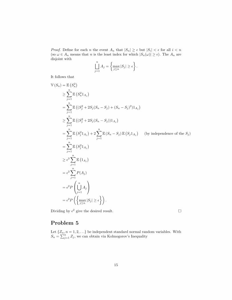
Proof. Define for each n the event An that |Sn| ≥ ε but |Si| < ε for all i < n(so ω ∈ An means that n is the least index for which |Sn(ω)| ≥ ε). The An aredisjoint with

n⊔j=1

Aj =

maxj≤n|Sj | ≥ ε

.

It follows that

V (Sn) = E(S2n

)≥

n∑j=1

E(S2n1Aj

)=

n∑j=1

E((S2j + 2Sj(Sn − Sj) + (Sn − Sj)2)1Aj

)≥

n∑j=1

E((S2j + 2Sj(Sn − Sj))1Aj

)=

n∑j=1

E(S2j 1Aj

)+ 2

n∑j=1

E (Sn − Sj)E(Sj1Aj

)(by independence of the Sj)

=

n∑j=1

E(S2j 1Aj

)≥ ε2

n∑j=1

E(1Aj)

= ε2n∑j=1

P (Aj)

= ε2P

n⋃j=1

Aj

= ε2P

(maxj≤n|Sj | ≥ ε

).

Dividing by ε2 give the desired result.

Problem 5

Let Zn, n = 1, 2, . . . be independent standard normal random variables. WithSn =

∑nj=1 Zj , we can obtain via Kolmogorov’s Inequality

15

P

maxj≤10|Sj | > 10

≤ V (S10)

102

=10

102

=1

10.

The following R program (which performs 100,000 experiments) estimatesthe probability as 0.00211, which is significantly lower than the bound providedby Kolmogorov.

loop <- 0

numLoop <- 100000

max <- 10

count <- 0

while (loop < numLoop)

v = rnorm(10,0,1)

pv <- vector()

i <- 1

while ( i <= 10 )

col <- 1

partial <- 0

while ( col <= i )

partial <- partial + v[col]

col <- col + 1

pv[i] <- abs(partial)

i <- i + 1

if (max(pv) > max) count <- count + 1

loop <- loop + 1

prob <- count / numLoop

print(prob)

Problem 6

Proposition 26. For a collection An, n ≥ 1 of events in some ambient prob-ability space,

P∪ni=1Ai ≥[E(∑ni=1 I(Ai))]

2

E[(∑ni=1 I(Ai))2]

.

16

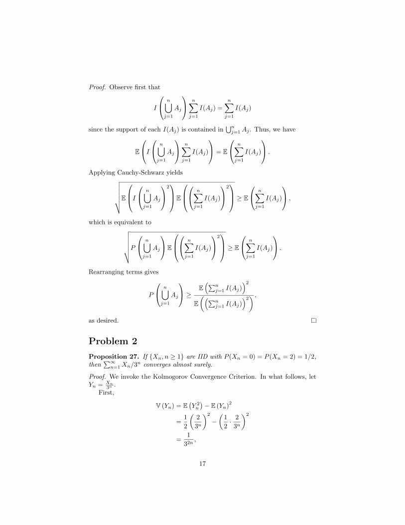
Proof. Observe first that

I

n⋃j=1

Aj

n∑j=1

I(Aj) =

n∑j=1

I(Aj)

since the support of each I(Aj) is contained in⋃nj=1Aj . Thus, we have

E

I n⋃j=1

Aj

n∑j=1

I(Aj)

= E

n∑j=1

I(Aj)

.

Applying Cauchy-Schwarz yields√√√√√√E

I n⋃j=1

Aj

2E

n∑j=1

I(Aj)

2 ≥ E

n∑j=1

I(Aj)

,

which is equivalent to√√√√√√P

n⋃j=1

Aj

E

n∑j=1

I(Aj)

2 ≥ E

n∑j=1

I(Aj)

.

Rearranging terms gives

P

n⋃j=1

Aj

≥ E(∑n

j=1 I(Aj))2

E((∑n

j=1 I(Aj))2) ,

as desired.

Problem 2

Proposition 27. If Xn, n ≥ 1 are IID with P (Xn = 0) = P (Xn = 2) = 1/2,then

∑∞n=1Xn/3

n converges almost surely.

Proof. We invoke the Kolmogorov Convergence Criterion. In what follows, letYn = Xn

3n .First,

V (Yn) = E(Y 2n

)− E (Yn)

2

=1

2

(2

3n

)2

−(

1

2· 2

3n

)2

=1

32n,

17

for all n. Thus, ∑n

V (Yn) =∑n

1

32n

=1

8<∞.

By the convergence criterion,∑n(Yn−E (Yn)) converges almost surely. Now,

E (Yn) =1

2· 2

3n

=1

3n.

Since∑n

13n = 1

2 <∞, it follows that∑n Yn converges almost surely.

Problem 3

Let Xn, n ≥ 1 be IID random variables taking values in the set S = 1, 2, . . . , 17.Define the discrete density (density with respect to counting measure) f0(y) =P (X1 = y), y ∈ S so that f0(y) ≥ 0 and

∑y∈S f0(y) = 1. Let f1 6= f0 be an-

other discrete density on S so that we also have f1(y) ≥ 0 and∑y∈S f1(y) = 1.

Set

Zn =

n∏i=1

f1(Xi)

f0(Xi), n ≥ 1.

The Zn, n ≥ 1 is called the likelihood ratio process.

Proposition 28. Under f0,Zn

a.s.−→ 0.

Proof. Define Yn = log(Zn), so that

Yn =

n∑i=1

log

(f1(Xi)

f0(Xi)

).

To show that Zna.s.−→ 0, we show equivalently that Yn

a.s.−→ −∞.

18

Applying Jensen’s Inequality, we have

Ef0[log

(f1(Xi)

f0(Xi)

)]< log

(Ef0

[f1(Xi)

f0(Xi)

])

= log

∑y∈S

(f1(y)

f0(y)

)f0(y)

= log

∑y∈S

f1(y)

= log(1)

= 0.

Now,

Ef0 (Yn) =

n∑i=1

Ef0[log

(f1(Xi)

f0(Xi)

)]< 0.

If the sum above diverges to −∞, then we are done. Suppose instead Ef0 (Yn)is equal to some finite, negative value µ (and so Ef0 |Yn| = −µ is also finite). Bythe Strong Law of Large Numbers,

Ynn

a.s.−→ µ.

Thus, Yn decreases without bound, and so Yna.s.−→ −∞.

Problem 4

Proposition 29. Let Xn, n ≥ 1 be IID random variables with P (Xn > x) =exp(−x), x ≥ 0. As n→∞,

maxi≤nXi

log(n)

a.s.−→ 1.

Proof. Let Yn = maxi≤nXi. We show that Ynlog(n)

a.s.−→ 1.

19

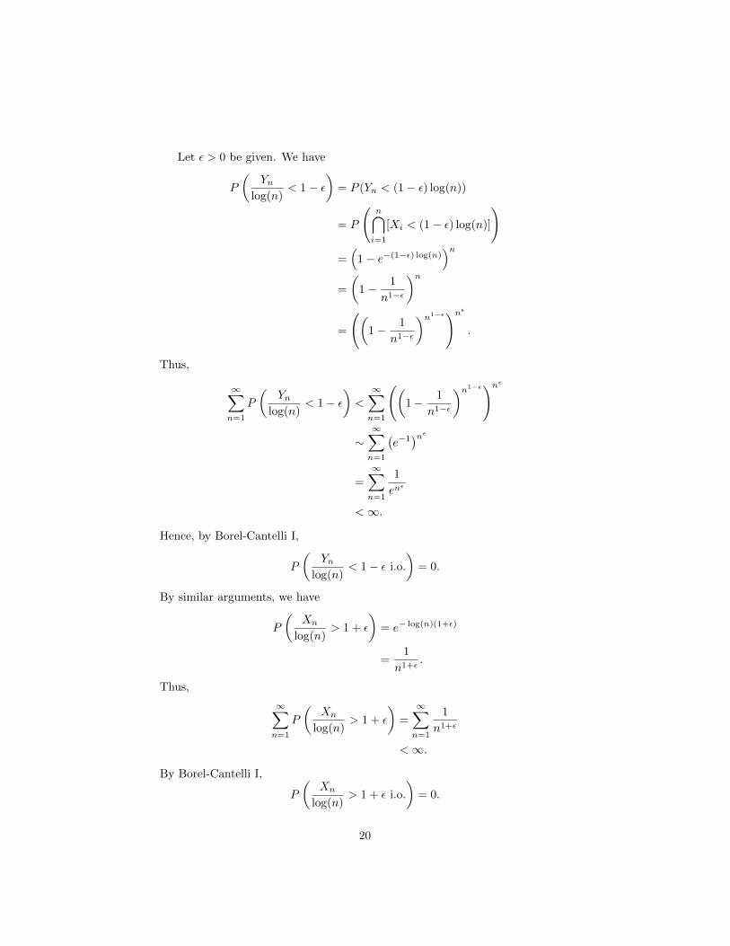
Let ε > 0 be given. We have

P

(Yn

log(n)< 1− ε

)= P (Yn < (1− ε) log(n))

= P

(n⋂i=1

[Xi < (1− ε) log(n)]

)=(

1− e−(1−ε) log(n))n

=

(1− 1

n1−ε

)n=

((1− 1

n1−ε

)n1−ε)nε.

Thus,

∞∑n=1

P

(Yn

log(n)< 1− ε

)<

∞∑n=1

((1− 1

n1−ε

)n1−ε)nε

∼∞∑n=1

(e−1)nε

=

∞∑n=1

1

enε

<∞.

Hence, by Borel-Cantelli I,

P

(Yn

log(n)< 1− ε i.o.

)= 0.

By similar arguments, we have

P

(Xn

log(n)> 1 + ε

)= e− log(n)(1+ε)

=1

n1+ε.

Thus,

∞∑n=1

P

(Xn

log(n)> 1 + ε

)=

∞∑n=1

1

n1+ε

<∞.

By Borel-Cantelli I,

P

(Xn

log(n)> 1 + ε i.o.

)= 0.

20

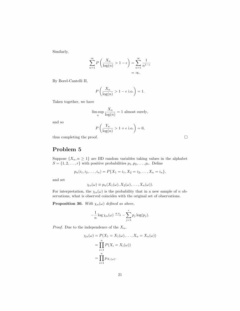
Similarly,

∞∑n=1

P

(Xn

log(n)> 1− ε

)=

∞∑n=1

1

n1−ε

=∞.

By Borel-Cantelli II,

P

(Xn

log(n)> 1− ε i.o.

)= 1.

Taken together, we have

lim supn

Xn

log(n)= 1 almost surely,

and so

P

(Yn

log(n)> 1 + ε i.o.

)= 0,

thus completing the proof.

Problem 5

Suppose Xn, n ≥ 1 are IID random variables taking values in the alphabetS = 1, 2, . . . , r with positive probabilities p1, p2, . . . , pr. Define

pn(i1, i2, . . . , in) = PX1 = i1, X2 = i2, . . . , Xn = in,

and setχn(ω) ≡ pn(X1(ω), X2(ω), . . . , Xn(ω)).

For interpretation, the χn(ω) is the probability that in a new sample of n ob-servations, what is observed coincides with the original set of observations.

Proposition 30. With χn(ω) defined as above,

− 1

nlogχn(ω)

a.s.−→ −r∑j=1

pj log(pj).

Proof. Due to the independence of the Xn,

χn(ω) = P (X1 = X1(ω), . . . , Xn = Xn(ω))

=

n∏i=1

P (Xi = Xi(ω))

=

n∏i=1

pXi(ω).

21

Now,

log(χn(ω)) =

n∑i=1

log(pXi(ω)).

Let Sn =∑ni=1 log(pXi(ω)). Since the Xi are IID, the log(pXi(ω)) terms are also

IID. Now,

E(log(pXi(ω))

)=

r∑j=1

pj log(pj),

which is finite. Thus, by the Strong Law of Large Numbers,

− 1

nlogχn(ω) = −Sn

na.s.−→ −E (Sn)

= −r∑j=1

pj log(pj),

as desired.

Problem 1

Let Sn have a binomial distribution with parameters n and θ ∈ (0, 1). By basicCentral Limit Theorem it is known that

Sn − nθ√nθ(1− θ)

⇒ N(0, 1).

Proposition 31. If Yn = log[Sn/(n− Sn)], then Yn ∼ AN(

θ1−θ ,

θn(1−θ)3

).

Proof. Observe first that, from the given weak convergence of Sn, we have

Snn − θ√θ(1−θ)n

⇒ N(0, 1),

so that Snn ∼ AN

(θ, θ(1−θ)n

).

Next, we write

Yn = log

(Snn

1− Snn

).

Define g(x) = log(

x1−x

), so that Yn = g

(Snn

). Now, g′(x) = 1

x(1−x) , which is

nonzero for all x ∈ (0, 1). By the Delta Method, we have Yn ∼ AN(

log(

θ1−θ

), 1nθ(1−θ)

).

22

Problem 2

Proposition 32. Let Xn, n = 1, 2, . . . be independent random variables suchthat PXn = n = 1/n = 1 − PXn = 0. The sequence Xn, n = 1, 2, . . .converges in probability, and thus weakly.

Proof. We show that Xnpr−→ 0. For any ε > 0, we have

limn→∞

P (|Xn − 0| > ε) = limn→∞

P (Xn = n)

= limn→∞

1

n

= 0.

Now, convergence in probability always implies weak convergence, and so theclaim is proven.

Problem 3

Proposition 33. Let Un, n = 1, 2, . . . be IID from a uniform distribution on[0, 1]. There exist sequences µn and σn such that[∏n

i=1 U1/ni

]− µn

σn

converges weakly to a non-degenerate random variable.

Proof. Let Xn = log(Ui), so that log(∏n

i=1 U1ni

)= 1

n

∑ni=1 log(Ui) = Xn. Let

µX = E (X1) and σ2X = V (X1) be the common mean and variance, respectively.

By the basic Central Limit Theorem, we have

√n

(Xn − µX

σX

)⇒ N(0, 1),

and so Xn ∼ AN(µX ,

σ2X

n

). Applying the Delta Method with g(x) = ex, we

have

eXn =

n∏i=1

U1ni ∼ AN

(eµX , e2µX

σ2X

n

).

The desired sequences are thus obtained by taking µn = eµX and σn = eµX σX√n

.

Problem 4

Let Xn, n = 1, 2, . . . be IID from a unit exponential distribution. For a fixedl, denote by X(l:n) the lth smallest among X1, X2, . . . , Xn where n ≥ l.

23

Proposition 34. The sequence nX(l:n) ⇒ Yl where Yl has a gamma distributionwith shape parameter l and scale parameter 1, that is,

PYl ≤ y =

∫ y

0

1

(l − 1)!wl−1 exp(−w)dw.

Proof. Define, for 1 ≤ i ≤ n, the spacings Di = (n− i+1)(X(i)−X(i−1)) (wherewe take D1 = nX(1)). By Renyi’s representation, we have that the Di are IID

unit exponential random variables. Observe that X(l:n) =∑li=1

Din−i . Thus,

nX(l:n) →∑li=1Di. It is known that the sum of l IID unit exponential random

variables has a gamma distribution with shape paramater l and scale parameter1, thus completing the proof.

Problem 5

For distribution functions F and G define

d(F,G) = infδ > 0 : ∀x ∈ <, F (x− δ)− δ ≤ G(x) ≤ F (x+ δ) + δ.

Proposition 35. On the space of distribution functions, d(·, ·) is a metric.

Proof. Let F , G, and H be distribution functions. We claim first that, wheneverd(F,G) < α,

F (x− α)− α ≤ G(x) ≤ F (x+ α) + α.

To see this, observe that, by definition of d(·, ·), there is 0 ≤ δ < α such that

F (x− δ)− δ ≤ G(x) ≤ F (x+ δ) + δ.

As F is an increasing function, the claim follows.We show now that the function d is symmetric. For any fixed α > d(F,G),

we haveF (x− α)− α ≤ G(x) ≤ F (x+ α) + α,

from which is follows that

G(x− α) ≤ F (x) + α

andF (x)− α ≤ G(x+ α).

Equivalently,G(x− α) ≤ F (x) ≤ G(x+ α) + α.

Thus, d(G,F ) ≤ α. Since alpha was arbitrary, we obtain that d(G,F ) ≤d(F,G). By the same argument, we also see that d(F,G) ≤ d(G,F ), and sod(F,G) = d(G,F ).

We show next that d(F,G) = 0 if and only if F = G. If F = G, then

F (x− 0)− 0 ≤ G(x) ≤ F (x+ 0) + 0,

24

and so d(F,G) = 0. If d(F,G) = 0, then we have

F (x− α)− α ≤ G(x) ≤ F (x+ α) + α,

for any α > 0. Since F is right continuous, we have G ≤ F . Now, by symmetry,we have also d(G,F ) = 0, and so the same argument gives F ≤ G. Thus,F = G.

Finally, we show that d satisfies the triangle inequality. Choose α > d(F,H)and β > d(H,G) and apply the initial claim to get

F (x− α)− α ≤ H(x) ≤ F (x+ α) + α

andH(x− β)− β ≤ G(x) ≤ H(x+ β) + β.

It follows that

G(x) ≤ H(x+ β) + β ≤ F (x+ α+ β) + α+ β

andG(x) ≥ H(x− β)− β ≥ F (x− α− β)− α− β.

Thus, d(F,G) ≤ α+ β. As α and β are arbitrary, we have

d(F,G) ≤ d(F,H) + d(H,G),

as desired.

Proposition 36. The metric d(·, ·) metrizes convergence in distribution. Thatis, for distribution functions Fn | n ∈ N and F ,

Fn ⇒ F if and only if d(Fn, F )→ 0.

Proof. (⇒) Let ε > 0 be given. Since F is a distibution function, there arecontinuity points a and b such that

0 ≤ F (x) ≤ ε

2for all x ∈ (−∞, a]

and1− ε

2≤ F (x) ≤ 1 for all x ∈ [b,∞).

Choose now a sequence xn of continuity points of F such that

a = x0 < x1 < · · · < xn = b

andxi − xi−1 < ε for all i.

Now,limn→∞

Fn(xi) = F (xi) for all i,

25

so there exists Nε such that

|Fn(xi)− F (xi)| ≤ε

2for all n ≥ Nε.

Let now x ∈ [xi−1, xi] ⊂ [a, b]. For n ≥ Nε, we have

Fn(x) ≤ Fn(xi) ≤ F (xi) +ε

2≤ F (x+ ε) + ε.

Similarly,

Fn(x) ≥ Fn(xi−1) ≥ F (xi−1)− ε

2≥ F (x− ε)− ε.

Thus, for all x ∈ [a, b] and all n ≥ Nε,

F (x− ε)− ε ≤ Fn(x) ≤ F (x+ ε) + ε.

For x ∈ (−∞, a), choose any continuity point x+ such that x < x+. Wehave for all n ≥ Nε,

Fn(x) ≤ Fn(x+) ≤ F (x+) +ε

2≤ ε,

and so |Fn(x)− F (x)| ≤ ε.For x ∈ (b,∞), choose any continuity point x− such that x− < x. We have

for all n ≥ Nε,Fn(x) ≥ Fn(x−) ≥ F (x−)− ε

2≥ 1− ε,

and so |Fn(x)− F (x)| ≤ ε.As ε is arbitrary, we have d(Fn, F )→ 0, as desired.(⇐) Let ε > 0 be given. There is Nε such that d(Fn, F ) < ε for all n ≥ Nε.

By earlier remarks, this implies

F (x− ε)− ε ≤ Fn(x) ≤ F (x+ ε) + ε

for all x ∈ R and n ≥ Nε. Hence,

F (x− ε)− ε ≤ lim infn→∞

Fn(x) ≤ lim supn→∞

Fn(x) ≤ F (x+ ε) + ε.

Now, for any continuity point x, we have

limε↓0

F (x− ε)− ε = limε↓0

F (x+ ε) + ε,

and so conclude that limn→∞ Fn(x) = F (x) for all continuity points x. That is,Fn ⇒ F .

26

Problem 6

Proposition 37. Let Xn, n = 1, 2, . . . be IID from a standard uniform dis-tribution. There exist sequences an and bn such that (Mn−an)/bn convergesweakly to a nondegenerate distribution, where Mn =

∨ni=1Xi = maxX1, X2, . . . , Xn.

Proof. Observe first that

P (Mn ≤ x) = P

((n∨i=1

Xi

)≤ x

)= P ((X1 ≤ x) and · · · and (Xn ≤ x))

=

n∏i=1

P (Xi ≤ x)

= xn.

We next compute the mean and variance of Mn via the probability densityfunction nxn−1:

E (Mn) =

∫ 1

0

xnxn−1 dx

=n

n+ 1

and

V (Mn) =

∫ 1

0

x2nxn−1 dx

=n

(n+ 1)2(n+ 2).

Considering only the order of the mean and variance, we claim that settingan = 1 and bn = 1

n achieves the desired result. To verify this, observe

P

(Mn − 1

1n

≤ x)

= P(Mn ≤ 1 +

x

n

)=(

1 +x

n

)n→ ex.

Problem 7

Proposition 38. If Xn ⇒ X0 and for some δ > 0, supn E[|Xn|2+δ

]<∞, then

E(Xn)→ E(X0) and V(Xn)→ V(X0).

27

Proof. Observe first that, by the Baby Skorohod Theorem, there are random

variables X#n such that, for each n, X#

nd= Xn and X#

na.s.−→ Xn. Hence, it is

equivalent to establish the desired results for X#n .

Since E(|X#

n |2+δ)<∞, the Crystal Ball Condition guarantees the families

X#n and (X#

n )2 are uniformly integrable. Now, uniform integrability com-bined with almost sure convergence implies convergence of expectations. That

is, E(X#n

)→ E

(X#

0

)and

V(X#n

)= E

((X#

n )2)

+ E(X#n

)2→ E

((X#

0 )2)

+ E(X#

0

)2(since both X#

n and (X#n )2 are u.i.)

= V(X#

0

),

as desired.

Problem 1

Let Xi, i = 1, 2, . . . , n be independent random variables with Xi having a normaldistribution with mean µi and variance σ2

i .

Proposition 39. The sum S =∑ni=1Xi is normally distributed with mean∑n

i=1 µi and variance∑ni=1 σ

2i .

Proof. (via convolutions) We demonstrate the result for the case where n = 2and appeal to induction for the general result.

Let f(x) = c1 exp(− (x−µ)2

2σ2

)and g(x) = c2 exp

(− (x−ν)2

2τ2

)be the probabil-

ity density functions of independent, normally distributed random variables Xand Y , respectively. We have

(f ∗ g)(x) =

∫Rf(u)g(x− u)du

= c

∫R

exp

(− (u− µ)2

2σ2

)exp

(− (x− ν − u)2

2τ2

)du (where c = c1c2)

= c

∫R

exp

(−τ

2(u− µ)2 + σ2(x− u− ν)2

2σ2τ2

).

Using a computer algebra system, one can rewrite the above as

c exp

(− (x− (µ+ ν))2

2(σ2 + τ2)

)∫Rh(u)du,

where h(u) does not depend on x. Hence, we obtain

(f ∗ g)(x) = c′ exp

(− (x− (µ+ ν))2

2(σ2 + τ2)

).

28

Therefore, X + Y is normally distributed with mean µ + ν and variance σ2 +τ2.

Proof. (via characteristic functions) We demonstrate the result for the casewhere n = 2 and appeal to induction for the general result.

Let φX(t) and φY (t) be the characteristic functions of indepdent, normallydistributed random variables X and Y , respectively. We have

φX+Y (t) = E (exp(it(X + Y )))

= E (exp(itX)) + E (exp(itY ))

= exp

(itµ− σ2t2

2

)+ exp

(itν − τ2t2

2

)= exp(it(µ+ ν)− (σ2 + τ2)t2

2.

Therefore, X + Y is normally distributed with mean µ + ν and variance σ2 +τ2.

Problem 2

A rv X has a Poisson distribution with rate λ if PX = k = exp(−λ)λk/k!, k =0, 1, 2, . . ..

Proposition 40. The characteristic function of X is exp(λ(exp(iu)− 1)).

Proof. Let φ(t) be the characteristic function of X. We have

φ(t) = E (exp(itX))

=

∞∑k=0

exp(−λ)λk

k!exp(iuk)

= exp(−λ)

∞∑k=0

(λ exp(iu))k

k!

= exp(λ(exp(iu)− 1)).

Proposition 41. Let S =∑ni=1Xi where Xi ∼ POI(λi). The random variable

S has a Poisson distribution with parameter∑ni=1 λi.

Proof. We demonstrate the result for the case where n = 2 and appeal toinduction for the general result.

29

Let X ∼ POI(λ1) and Y ∼ POI(λ2) and let fX and fY be their respectiveprobability density functions. We have

P (X + Y = k) =

k∑j=0

fX(j)fY (k − j)

=

k∑j=0

λj1j!e−λ1

λk−j2

(k − j)!e−λ2

= e−(λ1+λ2)k∑j=0

λj1j!

λk−j2

(k − j)!

= e−(λ1+λ2)(λ1 + λ2)k

k!,

where the last equality results from an application of the binomial theorem.

Problem 3

A rv X is said to have a gamma distribution with shape parameter α(α > 0)and scale parameter λ(λ > 0) if its density function (wrt Lebesgue measure) is

f(x) =λα

Γ(α)xα−1 exp−λx, x ≥ 0.

We shall write in this case X ∼ Γ(α, λ).

Proposition 42. The characteristic function of X is(1− it

λ

)−α.

Proof. We have

E(eitX

)=

∫ ∞0

eityλα

Γ(α)yα−1e−λydy

=

∫ ∞0

λα

Γ(α)yα−1e−(λ−it)ydy

=λα

(λ− it)α

∫ ∞0

(λ− it)α

Γ(α)yα−1e−(λ−it)ydy

=λα

(λ− it)α

=

(1− it

λ

)−α.

30

Proposition 43. Let Xi ∼ Γ(αi, λ), i = 1, 2, . . . , n and assume that they areindependent. Let also S =

∑ni=1Xi. The characteristic function of S is

n∏i=1

(1− it

λ

)−αiProof. We have

E(eitS

)=

n∏i=1

eitXi

=

n∏i=1

(1− it

λ

)−αi.

Remark 1. To determine the distribution of S, we first obtain the density fvia

f(x) =1

2π

∫ ∞0

e−iyxφS(y)dy

=1

2π

∫ ∞0

e−iyxn∏i=1

(1− iy

λ

)−αidy.

The distribution F (u) is thus given by

F (u) =1

2π

∫ u

0

∫ ∞0

e−iyxn∏i=1

(1− iy

λ

)−αidydx

=1

2π

∫ ∞0

∫ u

0

e−iyxn∏i=1

(1− iy

λ

)−αidxdy

=1

2π

∫ ∞0

n∏i=1

(1− iy

λ

)−αi ∫ u

0

e−iyxdxdy

=1

2π

∫ ∞0

n∏i=1

(1− iy

λ

)−αi (e−iyu − 1

−iy

)dy

I do not see how to further simplify the expression above.

Problem 4

Let Xn, n = 1, 2, 3, . . . be IID rvs with P (Xn = −1) = P (Xn = +1) = 1/2, n =1, 2, . . .. The Cantor random variable on [−1/2, 1/2] is defined to be

C =

∞∑n=1

Xn

3n.

31

Proposition 44. The characteristic function of C is∏∞i=1 cos

(t3n

).

Proof. We have

E

(exp

(it

∞∑n=1

Xn

3n

))= E

( ∞∏n=1

exp

(itXn

3n

))

=

∞∏n=1

E(

cos

(Xnt

3n

)+ i sin

(Xnt

3n

))

=

∞∏n=1

cos

(t

3n

),

where the last equality makes use of the fact that P (Xn = 1) = P (Xn = −1) =12 .

Proposition 45. For all t ∈ R,

sin t

t=

∞∏n=1

cos

(t

2n

).

Proof. Let Z =∑∞n=1

Xn2n . By the previous result, we have

E

(exp

(it

∞∑n=1

Xn

2n

))=

∞∏n=1

cos

(t

2n

).

On the other hand,

E

(exp

(it

∞∑n=1

Xn

2n

))=

∞∑n=0

(it)n

n!E (Zn)

=

∞∑n=0n even

(it)n

n!E (Zn)

=

∞∑j=0

(−1)jt2j

(2j)!E(Z2j)

=1

t

∞∑j=0

(−1)jt2j+1

(2j)!

1

2j + 1

=sin t

t.

Problem 5

Let X1, X2, . . . , Xn be IID with a standard Cauchy distribution, that is, thecommon density with respect to Lebesgue measure is f(x) = 1/[π(1 + x2)] forx ∈ <. As we have seen in class the chf of X is exp−|t|.

32

Proposition 46. Let Xn =∑nj=1

Xjn . The distribution of Xn is given by

Proof. Given iid random variables with common characteristic function φX , wehave

φXn(t) = E(exp(itXn)

)= E

(exp

(itSnn

))= e−nE (exp(itSn))

= e−nφX(t)n

= e−ne−n|t|

= e−|t|

= φX(t).

Thus, Xn is distributed identically to each of the Xi.

Problem 1

Let Xn, n ≥ 1 be independent random variables with E(Xn) = 0 and V(Xn) =σ2n <∞. Let s2n =

∑ni=1 σ

2i .

Proposition 47. If there exists a δ > 0 such that, as n→∞,∑ni=1 E|Xi|2+δ

s2+δn

→ 0,

then the Lindeberg condition below holds:

∀ε > 0 : limn→∞

1

s2n

n∑i=1

E[X2i I|Xi| > εsn

]→ 0.

Proof. Let ε > 0 be given. It follows directly that

1

s2n

n∑i=1

E(X2i I|Xi| > εsn

)=

n∑i=1

E

(∣∣∣∣Xi

sn

∣∣∣∣2 I|Xi| > εsn

)

≤n∑i=1

E

(∣∣∣∣Xi

sn

∣∣∣∣2 ∣∣∣∣ Xi

εsn

∣∣∣∣δ I|Xi| > εsn

)

≤ 1

εδ

∑ni=1 E|Xi|2+δ

s2+δn

→ 0.

Remark 2. Define Sn =∑ni=1Xi. Since the Lindeberg condition holds for

Xn, the Lindeberg-Feller central limit theorem implies that Snsn⇒ N(0, 1).

33

Problem 2

Let Xn, n ≥ 1 be a sequence of independent random variables with mean zeroand variance σ2

n.

Proposition 48. Even if there exists a B > 0 such that ∀n : 1B ≤ σ2

n ≤ B, itdoes not follow that ∑n

i=1Xi√∑ni=1 σ

2i

⇒ N(0, 1). (1)

Proof. For a counterexample, define Xn = nI([0, 1n2 ])−nI([1− 1

n2 , 1]). We have,for all n,

E (Xn) = n · 1

n2− n · 1

n2

= 0

and

V (Xn) = E(X2n

)+ E (Xn)

2

= n2 · 1

n2+ n2 · 1

n2

= 2.

Let now Yn =∑nk=1Xk√∑nk=1 σ

2k

. For all n, Yn is equal to zero on the interval [ 14 ,34 ].

Thus, the distribution of the limiting random variable is constant on this inter-val, and so in particular is not normal.

Proposition 49. If, in addition, for some B <∞, ∀n : P|Xn| ≤ B = 1, ie.,the rvs are bounded, then (1) holds.

Proof. We establish the condition in Problem 1 and then appeal to the Lindeberg-Feller central limit theorem.

We have ∑ni=1 E

(|Xi|2+δ

)s2+δn

≤∑ni=1 E

(B2+δ

)(nB

)2+δ=nB2+δ

n2+δ

B2+δ

→ 0.

34

Problem 3

Suppose that Ys has a Poisson distribution with parameter s, not necessarily aninteger, so that

PYs = k =exp(−s)sk

k!, k = 0, 1, 2, . . . .

Proposition 50. As s→∞,

Ys − s√s⇒ N(0, 1).

Proof. Let Zs = Ys−s√s

. By the Uniqueness Theorem, it suffices to show that

the characteristic function of Zs converges to the characteristic function of astandard normal random variable.

We have

φZs(t) = φYs

(t√s

)exp(−it

√s)

= exp(s(e

it√s − 1)

)exp(−it

√s)

= exp(se

it√s − s− it

√s).

Taking logarithms, we proceed by showing the exponent converges to − t2

2 .

seit√s − s− it

√s = s

∞∑k=0

(it)k

(√s)kk!

− s− it√s

= s

(1 +

it√s− t2

2s− it3

6s32

+ · · ·)− s− it

√s

=

(s+ it

√s− t2

2− it3

6s12

+ · · ·)− s− it

√s

= − t2

2− it3

6s12

+ · · · .

Since t is constant, the above converges to − t2

2 as s→∞, as desired.

Problem 4

Let Xn, n ≥ 1 be independent random variables with Xn ∼ N(0, σ2n). Let

s2n =∑ni=1 σ

2i and Sn =

∑ni=1Xi.

Proposition 51. If the σ2n are chosen such that maxi≤n σ

2i /s

2n does not converge

to zero as n→∞, then the Lindeberg condition does not hold.

35

Proof. Define σk = 2−(k−1). We have, for all n,

maxi≤n

σ2i

s2n=

1∑nk=1 2−(k−1)

=1

2,

and so maxi≤nσ2i

s2ndoes not converge to zero.

As for the Lindeberg condition, observe first that sn →√22 . Choose ε0 such

that P|X1| > ε0√22 > 0 (such ε0 exists since X1 is not identically zero). We

have, for all n,

n∑i=1

E[X2i I|Xi| > ε0sn

]≥ E

[X2

1I|X1| > ε0sn]

→ E

[X2

1I

|X1| > ε0

√2

2

].

By our choice of ε0, the expectation above is equal to some positive constantnot depending on n. Therefore, the Lindeberg condition does not hold.

Proposition 52. For the choice of σ2n in the proposition above, we have Sn/sn ⇒

N(0, 1). [Remark: This shows that the Lindeberg condition is not necessary forthe CLT to hold.]

Proof. We know that Sn ∼ N(0, s2n), and so the characteristic function φSn(t) =exp

(− 1

2 t2s2n). Let now Yn = Sn

sn. We have

φYn(t) = φSn

(t

sn

)= exp

(−1

2

(t

sn

)2

s2n

)

= exp

(− t

2

2

).

Therefore, by the Uniqueness Theorem, Snsn

converges to a standard normalrandom variable.

Proposition 53. For the choice of σ2n in the above proposition, the following

condition does not hold:

∀ε > 0,maxi≤n

P|Xi| > εsn → 0.

36

Proof. Choose ε0 such that P|X1| > ε0√22 > 0 (such ε0 exists since X1 is not

identically zero). We have, for all n,

maxi≤n

P|Xi| > ε0sn ≥ P|X1| > ε0sn

→ P

|X1| > ε0

√2

2

.

By our choice of ε0, the probability above is equal to some positive constant notdepending on n. Therefore, the condition does not hold.

37