Math 1060 Lecture 6 Continuity - Chris...
45
Math 1060 Lecture 6 Continuity
Transcript of Math 1060 Lecture 6 Continuity - Chris...
Math 1060
Lecture 6Continuity
Outline
Summary of last lecture
Continuity at a pointMotivationDiscontinuitiesLeft- and right-continuity
ContinuityDefinition and intuitionExamples of continuous functionsThe intermediate value theorem
Pathological examples

Summary of last lecture
I Described the ε-δ definition of limits:
We say limx→a
f (x) = L if for every ε > 0 there exists a
δ > 0 such that |f (x)− L| < ε whenever0 < |x − a| < δ.
I Given a particular ε0 > 0, showed how to determine, for somesimple functions, the δ so that 0 < |x − a| < δ implies|f (x)− L| < ε0.
Work “backwards” from |f (x)− L| < ε to determinewhat you think δ should be, then verify that0 < |x − a| < δ does indeed imply |f (x)− L| < ε.
I Used the ε-δ definition to prove some of the limit laws fromearlier in the week.
I Described the ε-δ definitions for left- and right-hand limits.
I Described the ε-δ definition of an infinite limit.
Motivation
Last week we saw that some functions f (x), like polynomials andrational functions, satisfied a very nice property:
If a is in the domain of f , then limx→a
f (x) = f (a).
This property is nice because it makes calculating limits easy.

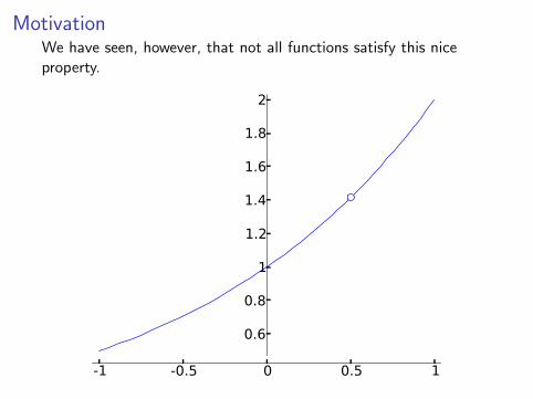
MotivationWe have seen, however, that not all functions satisfy this niceproperty.
-1 -0.5 0.5 1
-1
-0.5
0.5
1
MotivationWe have seen, however, that not all functions satisfy this niceproperty.
-1 -0.5 0 0.5 1
0.6
0.8
1
1.2
1.4
1.6
1.8
2
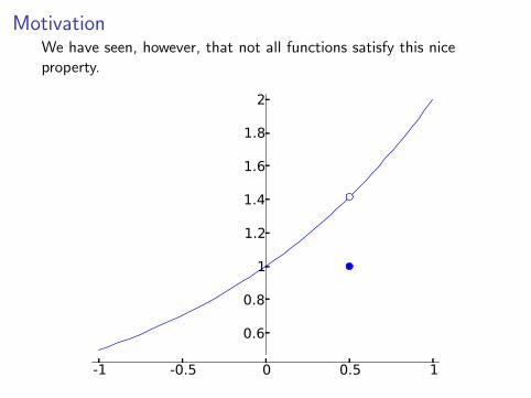
MotivationWe have seen, however, that not all functions satisfy this niceproperty.
-1 -0.5 0 0.5 1
0.6
0.8
1
1.2
1.4
1.6
1.8
2
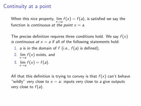
Continuity at a point
When this nice property, limx→a
f (x) = f (a), is satisfied we say the
function is continuous at the point x = a.
The precise definition requires three conditions hold. We say f (x)is continuous at x = a if all of the following statements hold:
1. a is in the domain of f (i.e., f (a) is defined),
2. limx→a
f (x) exists, and
3. limx→a
f (x) = f (a).
All that this definition is trying to convey is that f (x) can’t behave“wildly” very close to x = a: inputs very close to a give outputsvery close to f (a).
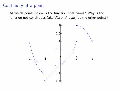
Continuity at a point
At which points below is the function continuous? Why is thefunction not continuous (aka discontinuous) at the other points?
-2 -1 1 2
-1.5
-1
-0.5
0.5
1
1.5
2
Continuity at a point
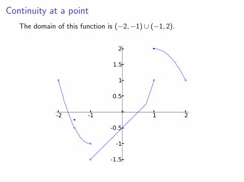
The domain of this function is (−2,−1) ∪ (−1, 2).
-2 -1 1 2
-1.5
-1
-0.5
0.5
1
1.5
2
Continuity at a point
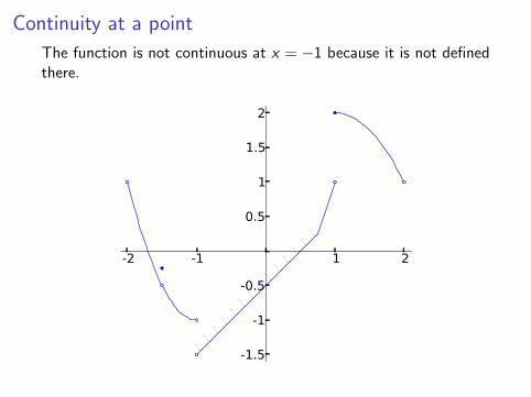
The function is not continuous at x = −1 because it is not definedthere.
-2 -1 1 2
-1.5
-1
-0.5
0.5
1
1.5
2
Continuity at a point
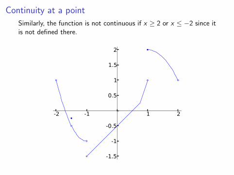
Similarly, the function is not continuous if x ≥ 2 or x ≤ −2 since itis not defined there.
-2 -1 1 2
-1.5
-1
-0.5
0.5
1
1.5
2
Continuity at a point
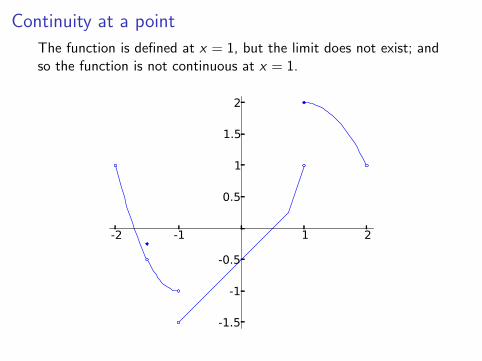
The function is defined at x = 1, but the limit does not exist; andso the function is not continuous at x = 1.
-2 -1 1 2
-1.5
-1
-0.5
0.5
1
1.5
2
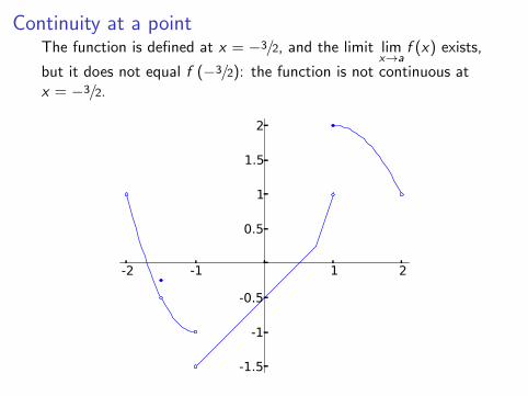
Continuity at a pointThe function is defined at x = −3/2, and the limit lim
x→af (x) exists,
but it does not equal f (−3/2): the function is not continuous atx = −3/2.
-2 -1 1 2
-1.5
-1
-0.5
0.5
1
1.5
2
Discontinuities
If f is not continuous at a, we say that a is a discontinuity of f .
Discontinuities occur because one of the three conditions in thedefinition of continuity at a point fail: Either
1. f is not defined at a,
2. the limit limx→a
f (x) does not exist, or
3. the function is defined and the limit does exist, butlimx→a
f (x) 6= f (a).
For the purposes of calculus, we like continuity at a point becauseit makes our lives a little easier. It is helpful, then, to know whichpoints cause us trouble: sometimes we would like to know where afunction is discontinuous.
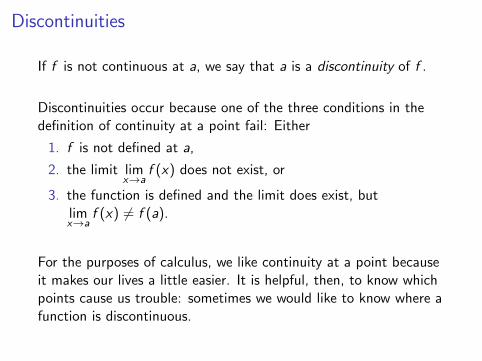
DiscontinuitiesExample: Where is the following function discontinuous, and whyis the function discontinuous at those points?
-2 -1.5 -1 -0.5 0.5 1
200
400
600
800
1000
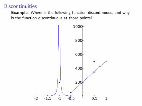
Discontinuities
Example: Where is the function f (x) = x2−4x2+2x
discontinuous, andwhy is the function discontinuous at those points?
We know that for rational functions, limx→a f (x) = f (a) whereverf (a) is defined. The only thing that can go wrong, then, is thatf (a) is undefined.
This happens precisely when the denominator is zero. Factoringthe denominator,
x2 + 2x = x(x + 2),
we see the function is discontinuous at x = 0 and at x = −2because that is where the function is undefined.
Discontinuities
Discontinuities can be classified as falling into a few differentcategories:
I Jump discontinuities
I Infinite discontinuities
I Removable discontinuities
Each of these three types corresponds to one of the threeconditions in the definition of continuity at a point failing.
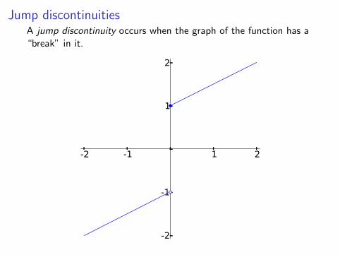
Jump discontinuitiesA jump discontinuity occurs when the graph of the function has a“break” in it.
-2 -1 1 2
-2
-1
1
2
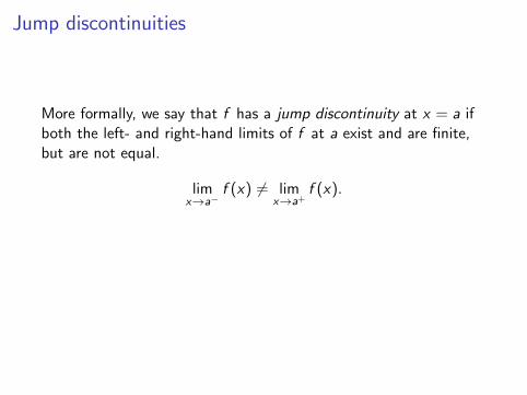
Jump discontinuities
More formally, we say that f has a jump discontinuity at x = a ifboth the left- and right-hand limits of f at a exist and are finite,but are not equal.
limx→a−
f (x) 6= limx→a+
f (x).
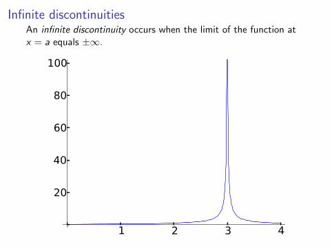
Infinite discontinuitiesAn infinite discontinuity occurs when the limit of the function atx = a equals ±∞.
1 2 3 4
20
40
60
80
100
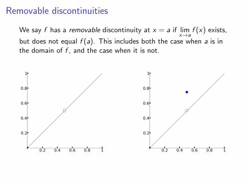
Removable discontinuities
We say f has a removable discontinuity at x = a if limx→a
f (x) exists,
but does not equal f (a). This includes both the case when a is inthe domain of f , and the case when it is not.
0.2 0.4 0.6 0.8 1
0.2
0.4
0.6
0.8
1
0.2 0.4 0.6 0.8 1
0.2
0.4
0.6
0.8
1
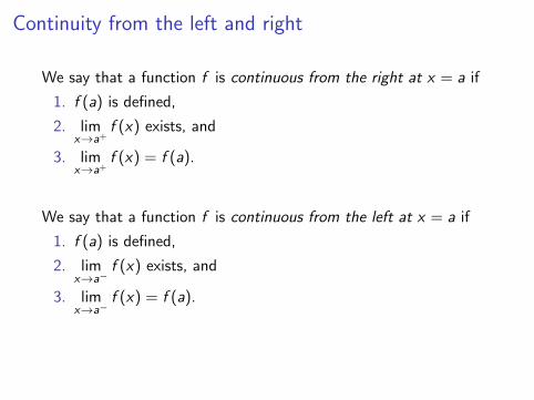
Continuity from the left and right
We say that a function f is continuous from the right at x = a if
1. f (a) is defined,
2. limx→a+
f (x) exists, and
3. limx→a+
f (x) = f (a).
We say that a function f is continuous from the left at x = a if
1. f (a) is defined,
2. limx→a−
f (x) exists, and
3. limx→a−
f (x) = f (a).
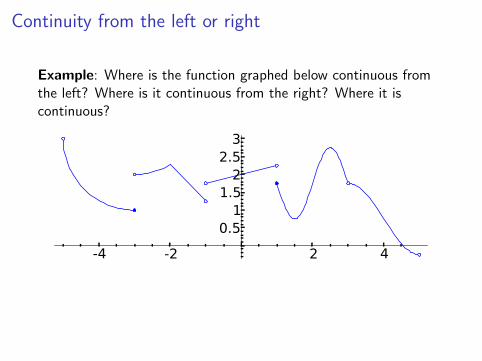
Continuity from the left or right
Example: Where is the function graphed below continuous fromthe left? Where is it continuous from the right? Where it iscontinuous?
-4 -2 2 4
0.51
1.52
2.53
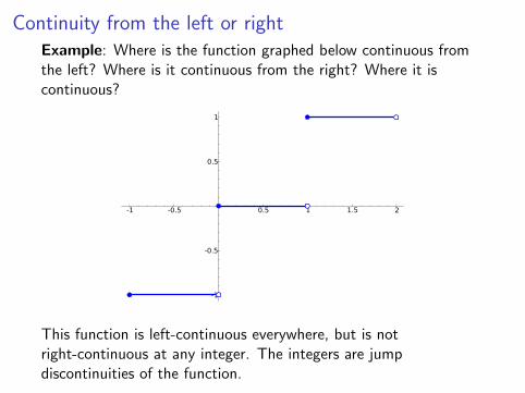
Continuity from the left or rightExample: Where is the function graphed below continuous fromthe left? Where is it continuous from the right? Where it iscontinuous?
This function is left-continuous everywhere, but is notright-continuous at any integer. The integers are jumpdiscontinuities of the function.
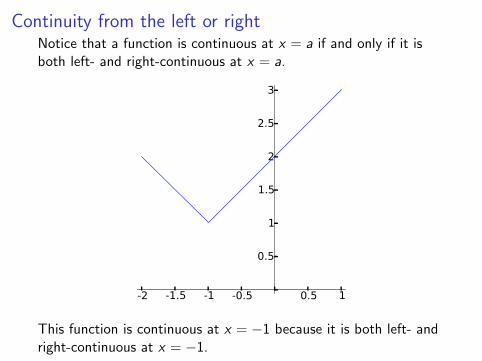
Continuity from the left or rightNotice that a function is continuous at x = a if and only if it isboth left- and right-continuous at x = a.
-2 -1.5 -1 -0.5 0.5 1
0.5
1
1.5
2
2.5
3
This function is continuous at x = −1 because it is both left- andright-continuous at x = −1.
Continuity
We defined continuity at a point earlier in the lecture. In thespecial situation that a function is continuous at every point whereit is defined we give the function a special name: continuous.
This might sound confusing because we are using the same wordto express two different ideas:
I continuous at a point: limx→a
f (x) = f (a)
I continuous: the continuous at a point definition applies atevery point where the function is defined.
The intuition behind continuity
When we say a function is continuous the intuitive idea is thatsmall changes in the input of the function, result in small changesin the output.
That is, if you change x just a little bit, then f (x) can only changea little bit as well.
The vast majority of functions modeling real-world, physicalphenomena (distance, position, velocity, acceleration, momentum,kinetic & potential energy, temperature, ...) are continuous.
Throughout your calculus careers, and in any applications ofcalculus (physics, engineering, computer science, ...), continuity isa very desirable property, and sometimes essential assumption, ofmost of the functions you will come in contact with.
ContinuityLuckily, lots of commonly used functions are continuous:
TheoremAll of the following types of functions are continuous:
1. Polynomials
2. Rational functions
3. Roots
4. Trigonometric functions
5. Inverse trig functions
6. Exponential functions
7. Logarithmic functions
Thus, for each of these types of functions,
limx→a
f (x) = f (a)
as long as f (a) is defined.
Continuity
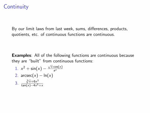
By our limit laws from last week, sums, differences, products,quotients, etc. of continuous functions are continuous.
Examples: All of the following functions are continuous becausethey are “built” from continuous functions:
1. x2 + sin(x)−√x cos(x)ex
2. arcsec(x)− ln(x)
3.3√x+6x3
tan(x)−4x5+x
Composition of continuous functions
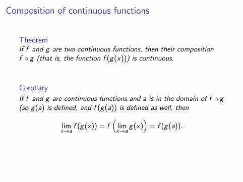
TheoremIf f and g are two continuous functions, then their compositionf ◦ g (that is, the function f (g(x))) is continuous.
Corollary
If f and g are continuous functions and a is in the domain of f ◦ g(so g(a) is defined, and f (g(a)) is defined as well, then
limx→a
f (g(x)) = f(
limx→a
g(x))
= f (g(a)).
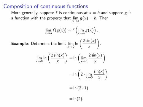
Composition of continuous functionsMore generally, suppose f is continuous at x = b and suppose g isa function with the property that lim
x→ag(x) = b. Then
limx→a
f (g(x)) = f(
limx→a
g(x)).
Example: Determine the limit limx→0
ln
(2 sin(x)
x
).
limx→0
ln
(2 sin(x)
x
)= ln
(limx→0
2 sin(x)
x
)
= ln
(2 · lim
x→0
sin(x)
x
)= ln (2 · 1)
= ln(2).
The intermediate value theorem
The intermediate value theorem is a simple idea that has manyinteresting consequences. Before giving the statement of thetheorem let’s think a little bit about the graphs of continuousfunctions whose domains are intervals.
If f (x) is defined for every x ∈ [a, b], then the graph y = f (x) hasno holes or jumps in it: it makes one “continuous” curve.
The intermediate value theorem
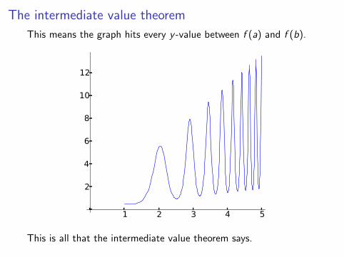
This means the graph hits every y -value between f (a) and f (b).
1 2 3 4 5
2
4
6
8
10
12
This is all that the intermediate value theorem says.
The intermediate value theorem
1 2 3 4 5
2
4
6
8
10
12
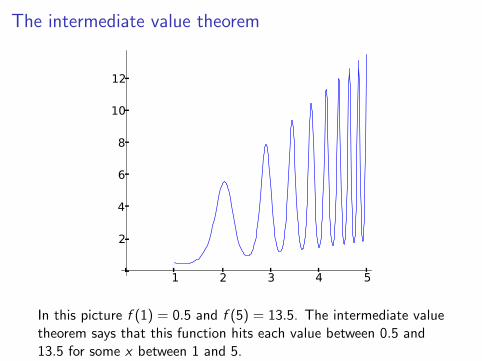
In this picture f (1) = 0.5 and f (5) = 13.5. The intermediate valuetheorem says that this function hits each value between 0.5 and13.5 for some x between 1 and 5.
The intermediate value theorem
TheoremLet f be a continuous function defined on the interval [a, b]. Forevery D between f (a) and f (b), there exists a x ∈ [a, b] such thatf (x) = D.
The intermediate value theorem seems like a simple observation,but it implies some very interesting, and non-obvious, facts.
The intermediate value theorem
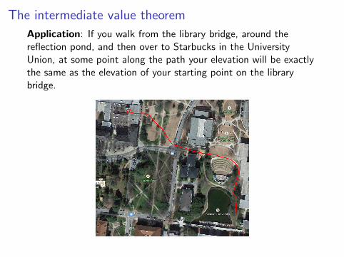
Application: If you walk from the library bridge, around thereflection pond, and then over to Starbucks in the UniversityUnion, at some point along the path your elevation will be exactlythe same as the elevation of your starting point on the librarybridge.
The intermediate value theorem
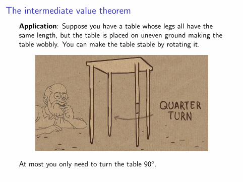
Application: Suppose you have a table whose legs all have thesame length, but the table is placed on uneven ground making thetable wobbly. You can make the table stable by rotating it.
At most you only need to turn the table 90◦.
Pathological examples
Sometimes in mathematics examples that are very strange andatypical are called pathological; these are usually verycounter-intuitive examples that show you how your intuition cansometimes lead you astray.
We will consider three such examples which should convince youthere are some very strange functions out there that don’t behavelike anything you’ve ever seen before. (I.e., all of your intuitiongoes out the window when considering such functions.)
A nowhere continuous function
In the examples of functions we’ve seen thus far, the functionswere continuous at “most” points: there were only finitely-manydiscontinuities.
There are functions, however, which are defined for every realnumber, but which are not continuous at any point; i.e., every realnumber is a discontinuity. Such functions are called nowherecontinuous.
Here’s one example of such a function:
f (x) =
{1 if x is irrational2 if x is rational
A nowhere continuous function
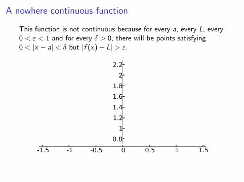
This function is not continuous because for every a, every L, every0 < ε < 1 and for every δ > 0, there will be points satisfying0 < |x − a| < δ but |f (x)− L| > ε.
-1.5 -1 -0.5 0 0.5 1 1.5
0.8
1
1.2
1.4
1.6
1.8
2
2.2
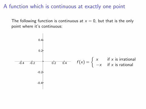
A function which is continuous at exactly one point
The following function is continuous at x = 0, but that is the onlypoint where it’s continuous:
-0.4 -0.2 0.2 0.4
-0.4
-0.2
0.2
0.4
f (x) =
{x if x is irrational−x if x is rational
A continuous function with no smooth components
We’ve seen that the graph of a continuous function can have sharpedges and corners, but in the examples thus far these corners havebeen few and far between?
Can the graph of such a function have infinitely many suchcorners?
Can the graph of such a function consist entirely of corners?
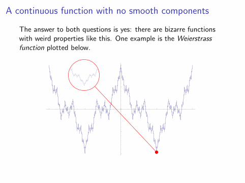
A continuous function with no smooth components
The answer to both questions is yes: there are bizarre functionswith weird properties like this. One example is the Weierstrassfunction plotted below.

Homework
Due Monday, September 8 :
I Read §2.5 in Stewart.I Homework set listed on the website (will appear
online late Wednesday / early Thursday)


![T P tt Δt tt - acclab.helsinki.fiknordlun/moldyn/lecture06.pdf · source: L.E. Reichl, A Modern Course in Statistical Physics] ... the chemical potential [cf. e.g. Mandl “Statistical](https://static.fdocument.org/doc/165x107/5b8140337f8b9a466b8bf338/t-p-tt-t-tt-knordlunmoldynlecture06pdf-source-le-reichl-a-modern.jpg)


![Lecture06 TeknikKloning.ppt [Read-Only]ocw.usu.ac.id/course/download/811-prinsip-bioteknologi/mipa_-_pb... · • Melakukan penyisipan bahan genetik operon galaktosa ... • Bahan](https://static.fdocument.org/doc/165x107/5c824b5809d3f27e788beaa8/lecture06-read-onlyocwusuacidcoursedownload811-prinsip-bioteknologimipa-pb.jpg)