Markov Chains8Tutorial #

Based on original slides of Ilan Gronau

Statistical Parameter EstimationReminder

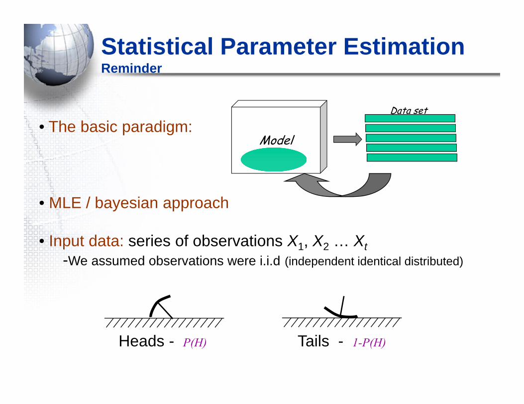
• The basic paradigm:

• MLE / bayesian approach

• Input data: series of observations X1, X2 … Xt-We assumed observations were i.i.d (independent identical distributed)

Data set

ModelParameters: Θ

Heads - P(H) Tails - 1-P(H)

Markov Process

3

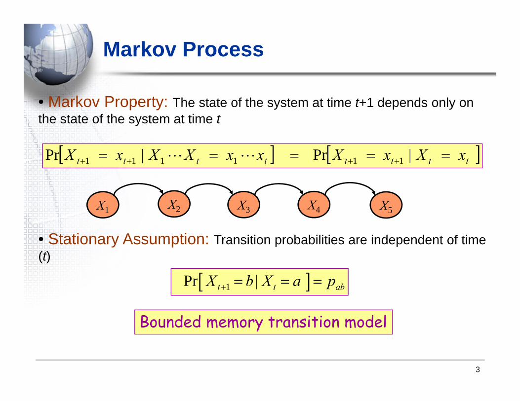
• Markov Property: The state of the system at time t+1 depends only on the state of the system at time t

X1 X2 X3 X4 X5

x | X x X x x X | X x X tttttttt 111111 PrPr

• Stationary Assumption: Transition probabilities are independent of time (t)

1Pr t t abX b | X a p

Bounded memory transition model

4

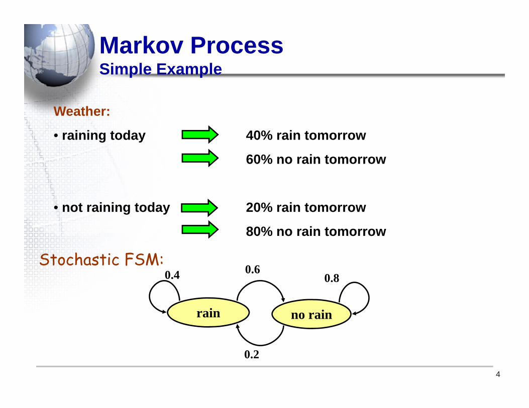
Weather:

• raining today 40% rain tomorrow

60% no rain tomorrow

• not raining today 20% rain tomorrow

80% no rain tomorrow

Markov ProcessSimple Example

rain no rain

0.60.4 0.8

0.2

Stochastic FSM:

8.02.06.04.0

P

5

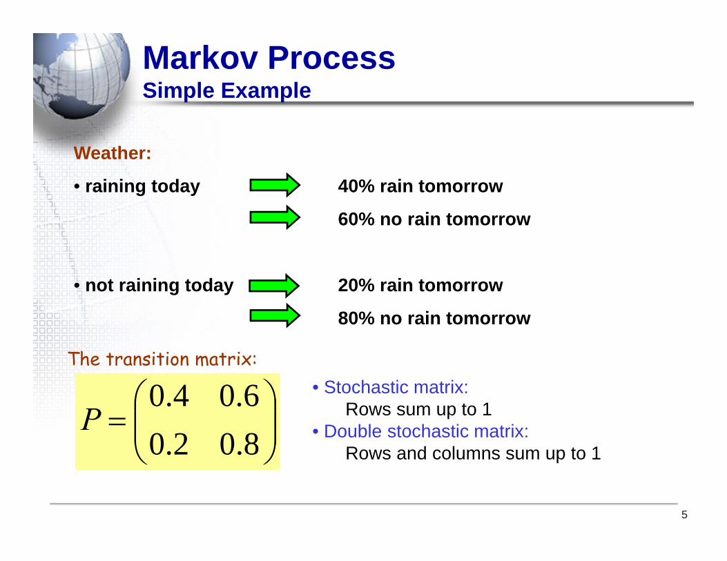
Weather:

• raining today 40% rain tomorrow

60% no rain tomorrow

• not raining today 20% rain tomorrow

80% no rain tomorrow

Markov ProcessSimple Example

• Stochastic matrix:Rows sum up to 1

• Double stochastic matrix:Rows and columns sum up to 1

The transition matrix:

6

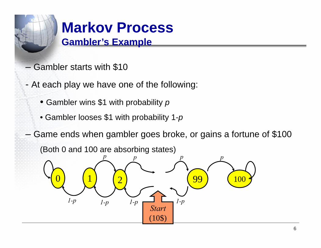
– Gambler starts with $10

- At each play we have one of the following:

• Gambler wins $1 with probability p

• Gambler looses $1 with probability 1-p

– Game ends when gambler goes broke, or gains a fortune of $100

(Both 0 and 100 are absorbing states)

0 1 2 99 100

p p p p

1-p 1-p 1-p 1-pStart (10$)

Markov ProcessGambler’s Example

1Pr t t abX b | X a p

7

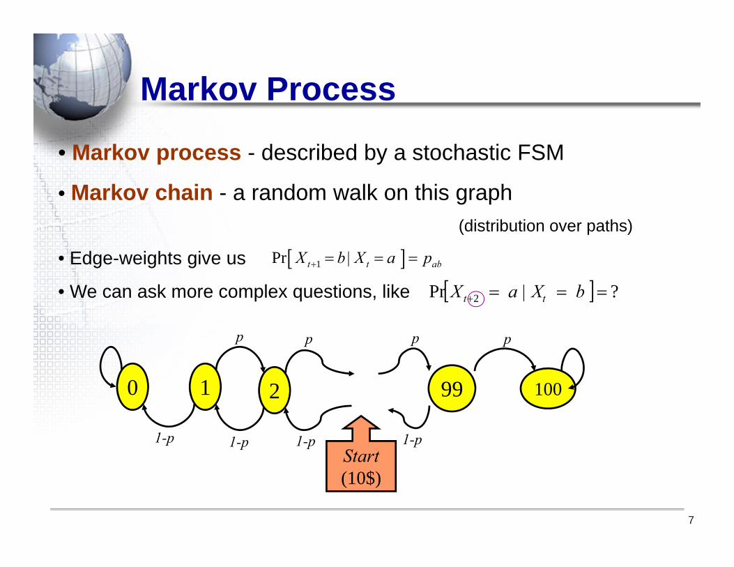
• Markov process - described by a stochastic FSM

• Markov chain - a random walk on this graph (distribution over paths)

• Edge-weights give us

• We can ask more complex questions, like

Markov Process

?Pr 2 b a | X X tt

0 1 2 99 100

p p p p

1-p 1-p 1-p 1-pStart (10$)

8

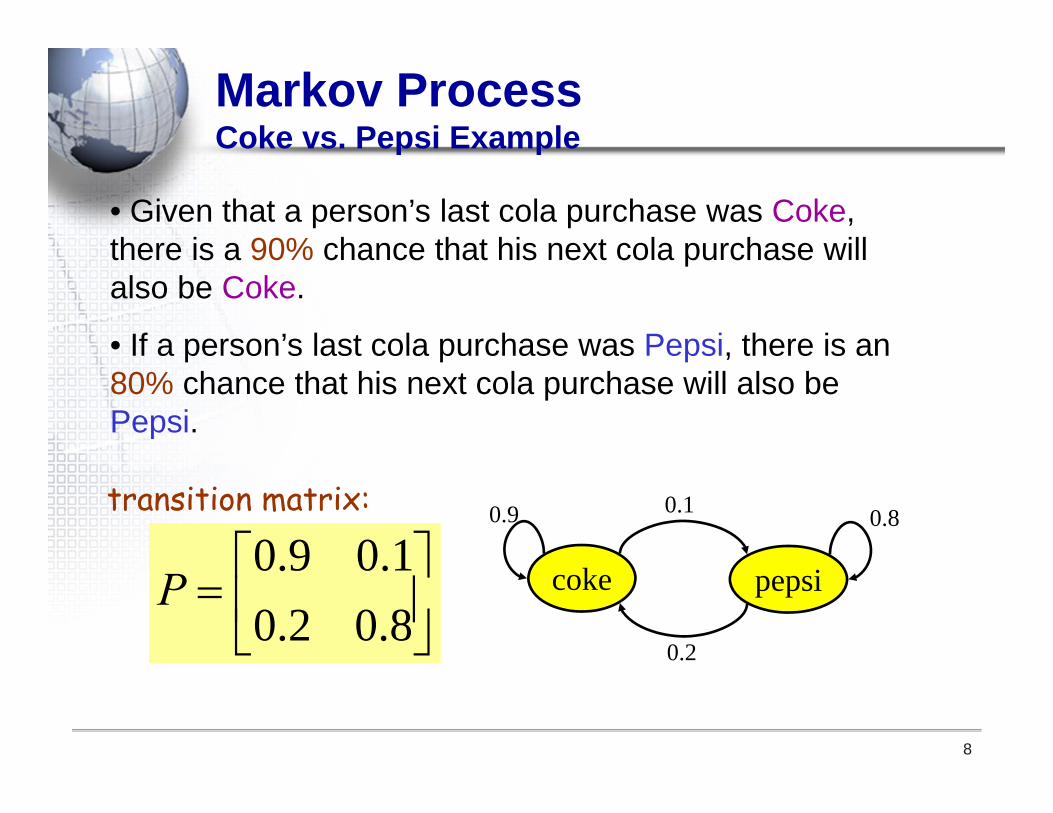
• Given that a person’s last cola purchase was Coke, there is a 90% chance that his next cola purchase will also be Coke.

• If a person’s last cola purchase was Pepsi, there is an 80% chance that his next cola purchase will also be Pepsi.

coke pepsi

0.10.9 0.8

0.2

Markov ProcessCoke vs. Pepsi Example

8.02.01.09.0

P

transition matrix:

9

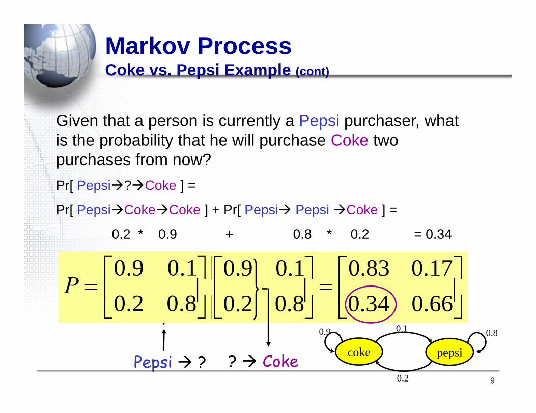
Given that a person is currently a Pepsi purchaser, what is the probability that he will purchase Coke two purchases from now?Pr[ Pepsi?Coke ] =

Pr[ PepsiCokeCoke ] + Pr[ Pepsi PepsiCoke ] =

0.2 * 0.9 + 0.8 * 0.2 = 0.34

66.034.017.083.0

8.02.01.09.0

8.02.01.09.02P

Markov ProcessCoke vs. Pepsi Example (cont)

Pepsi ? ? Coke

8.02.01.09.0

P

coke pepsi

0.10.9 0.8

0.2

10

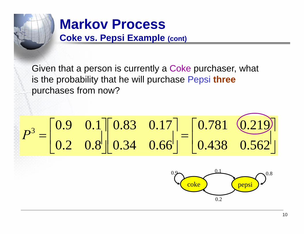
Given that a person is currently a Coke purchaser, what is the probability that he will purchase Pepsi threepurchases from now?

Markov ProcessCoke vs. Pepsi Example (cont)

562.0438.0219.0781.0

66.034.017.083.0

8.02.01.09.03P

coke pepsi

0.10.9 0.8

0.2

Markov ProcessCoke vs. Pepsi Example (cont)

8.02.01.09.0

P

11

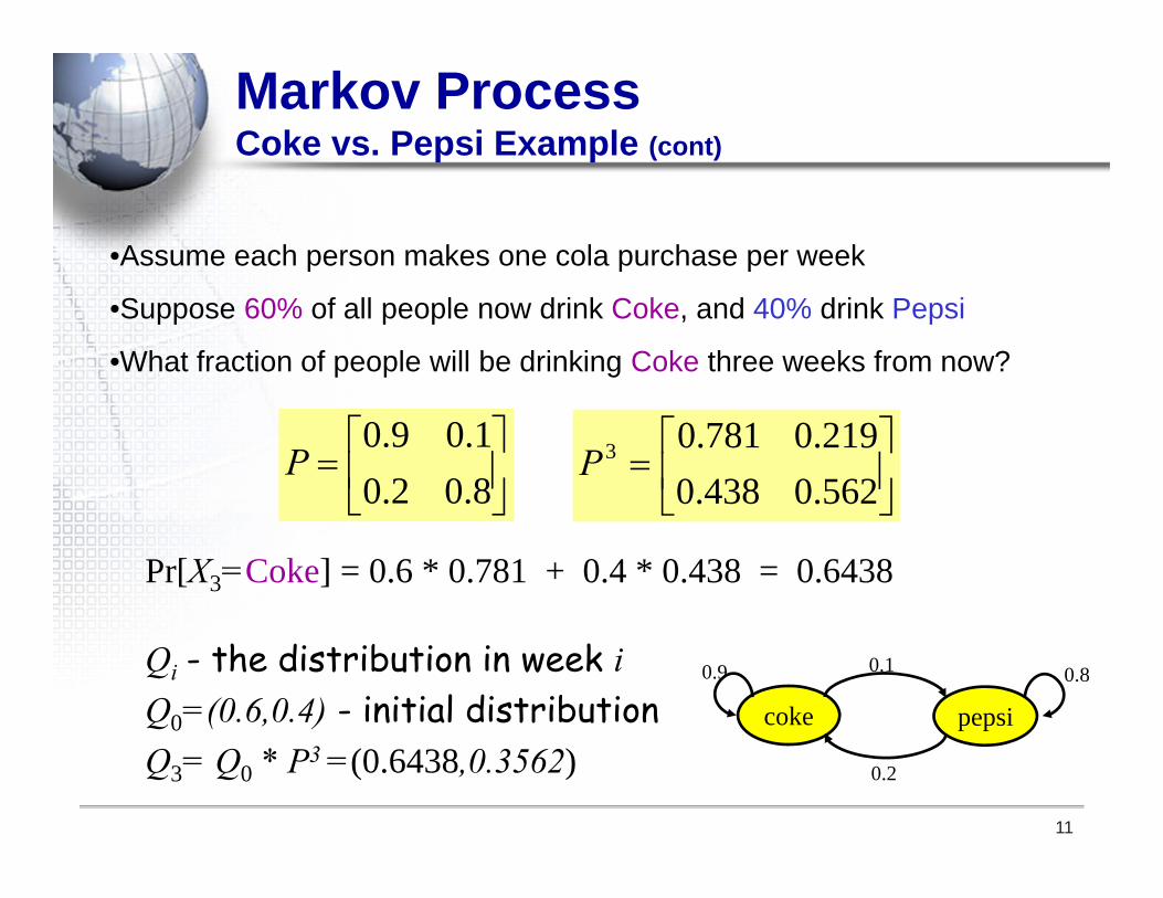
•Assume each person makes one cola purchase per week

•Suppose 60% of all people now drink Coke, and 40% drink Pepsi

•What fraction of people will be drinking Coke three weeks from now?

562.0438.0219.0781.03P

Pr[X3=Coke] = 0.6 * 0.781 + 0.4 * 0.438 = 0.6438

Qi - the distribution in week iQ0=(0.6,0.4) - initial distributionQ3= Q0 * P3 =(0.6438,0.3562)

coke pepsi

0.10.9 0.8

0.2

Markov ProcessCoke vs. Pepsi Example (cont)

8.02.01.09.0

P

12

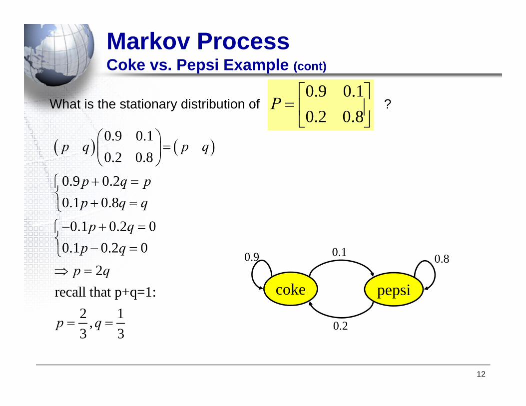
What is the stationary distribution of ?

0.9 0.1

0.2 0.8

0.9 0.20.1 0.8

0.1 0.2 00.1 0.2 0

2recall that p+q=1:

2 1,3 3

p q p q

p q pp q q

p qp q

p q

p q

coke pepsi

0.10.9 0.8

0.2

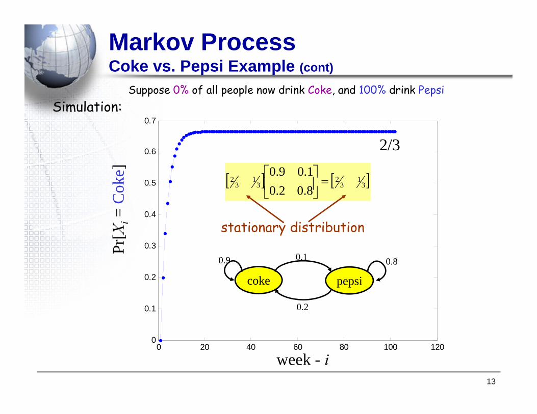
0 20 40 60 80 100 1200

0.1

0.2

0.3

0.4

0.5

0.6

0.7

13

Simulation:

week - i

Pr[X

i=

Cok

e]2/3

31

32

31

32

8.02.01.09.0

stationary distribution

coke pepsi

0.10.9 0.8

0.2

Markov ProcessCoke vs. Pepsi Example (cont)

Suppose 0% of all people now drink Coke, and 100% drink Pepsi

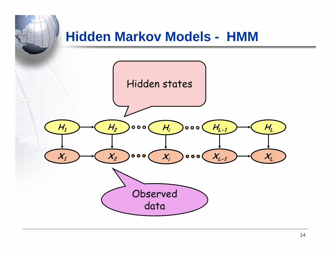
Hidden Markov Models - HMM

14

X1 X2 XL-1 XLXi

Hidden states

Observed data

H1 H2 HL-1 HLHi

15

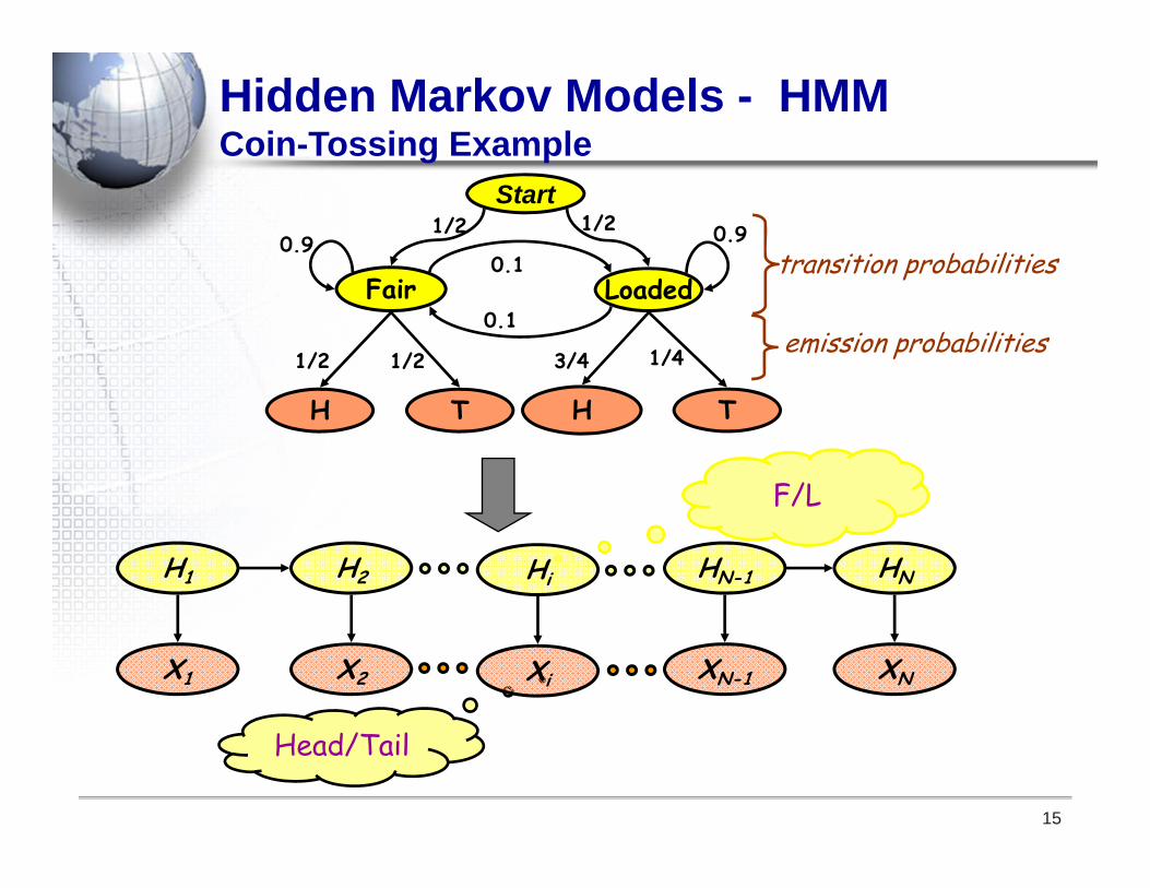
Hidden Markov Models - HMMCoin-Tossing Example

F/L

Head/Tail

X1 X2 XN-1 XNXi

H1 H2 HN-1 HNHi

transition probabilities

emission probabilities

0.9

Fair Loaded

H HT T

0.90.1

0.1

1/2 1/43/41/2

Start1/2 1/2

16

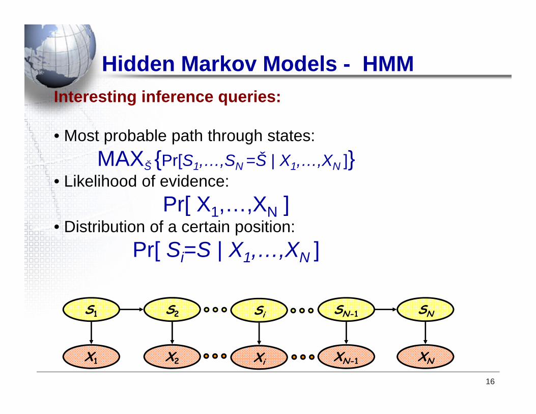
Hidden Markov Models - HMMInteresting inference queries:

• Most probable path through states: MAXŠ {Pr[S1,…,SN =Š | X1,…,XN ]}

• Likelihood of evidence:Pr[ X1,…,XN ]

• Distribution of a certain position:Pr[ Si=S | X1,…,XN ]

X1 X2 XN-1 XNXi

S1 S2 SN-1 SNSi

17

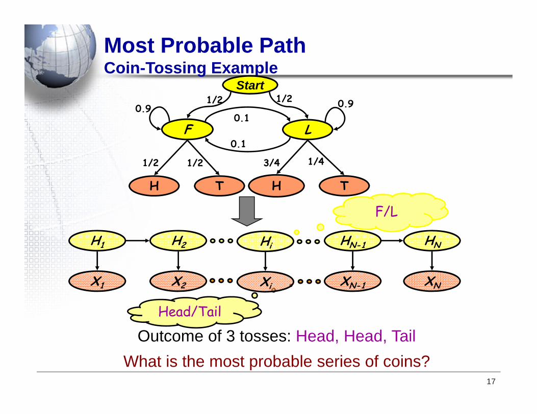
Most Probable PathCoin-Tossing Example

F/L

Head/Tail

X1 X2 XN-1 XNXi

H1 H2 HN-1 HNHi

0.9

F L

H HT T

0.90.1

0.1

1/2 1/43/41/2

Start1/2 1/2

Outcome of 3 tosses: Head, Head, TailWhat is the most probable series of coins?

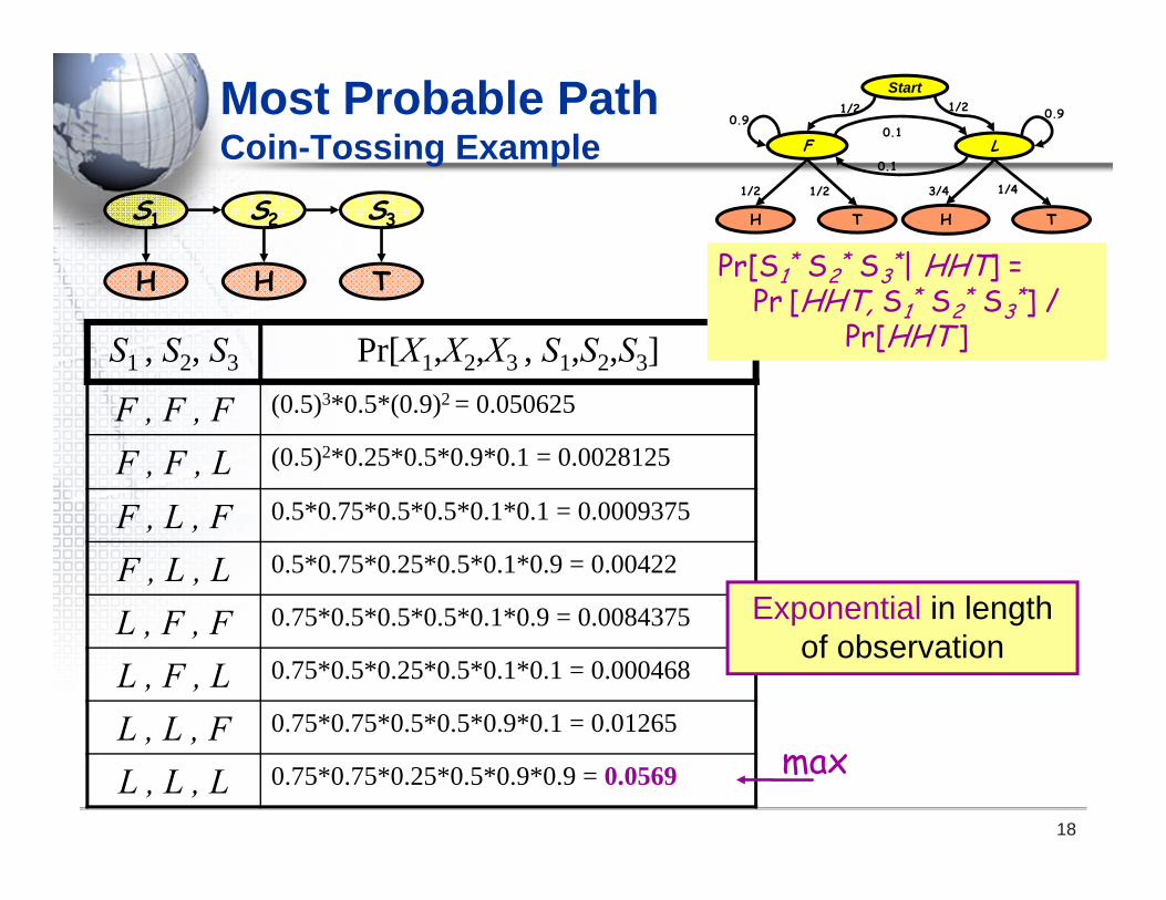
Most Probable PathCoin-Tossing Example

18

S1 , S2, S3 Pr[X1,X2,X3 , S1,S2,S3]

F , F , F (0.5)3*0.5*(0.9)2 = 0.050625

F , F , L (0.5)2*0.25*0.5*0.9*0.1 = 0.0028125

F , L , F 0.5*0.75*0.5*0.5*0.1*0.1 = 0.0009375

F , L , L 0.5*0.75*0.25*0.5*0.1*0.9 = 0.00422

L , F , F 0.75*0.5*0.5*0.5*0.1*0.9 = 0.0084375

L , F , L 0.75*0.5*0.25*0.5*0.1*0.1 = 0.000468

L , L , F 0.75*0.75*0.5*0.5*0.9*0.1 = 0.01265

L , L , L 0.75*0.75*0.25*0.5*0.9*0.9 = 0.0569 max

H H

S1 S2

T

S3

0.9

F L

H HT T

0.90.1

0.1

1/2 1/43/41/2

Start1/2 1/2

Exponential in length of observation

Pr[S1* S2

* S3*| HHT] =

Pr [HHT, S1* S2

* S3*] /

Pr[HHT ]