LOFAR Status Meeting  —  Oct 14, 2015

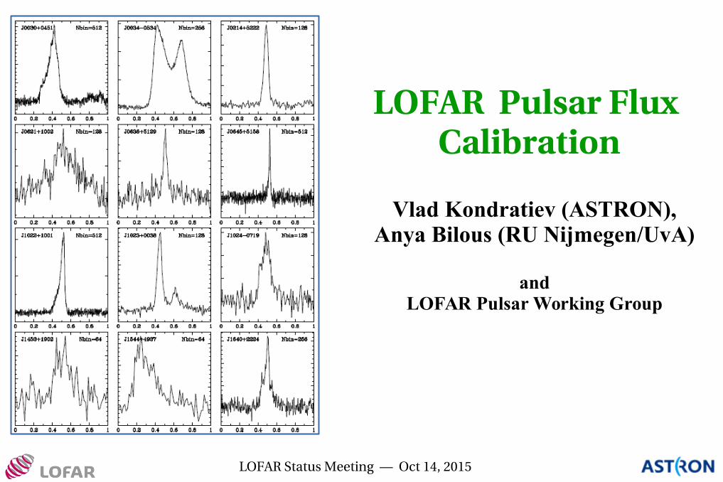
LOFAR  Pulsar Flux Calibration

Vlad Kondratiev (ASTRON),Anya Bilous (RU Nijmegen/UvA)

andLOFAR Pulsar Working Group

Flux calibration 

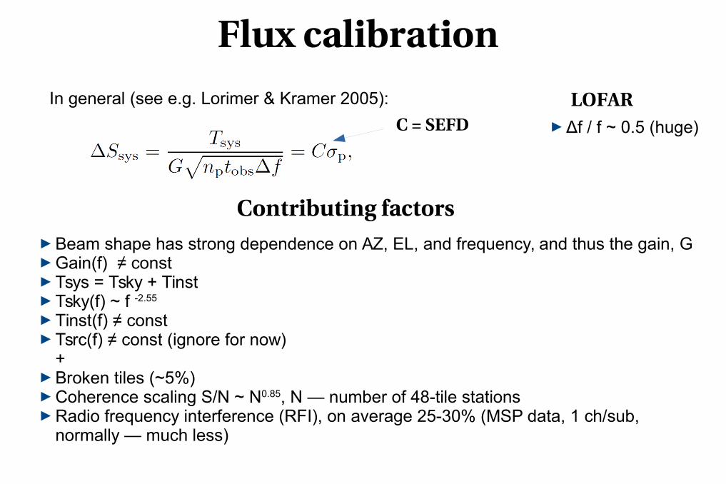
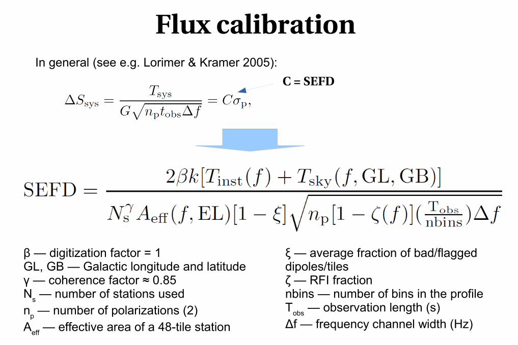
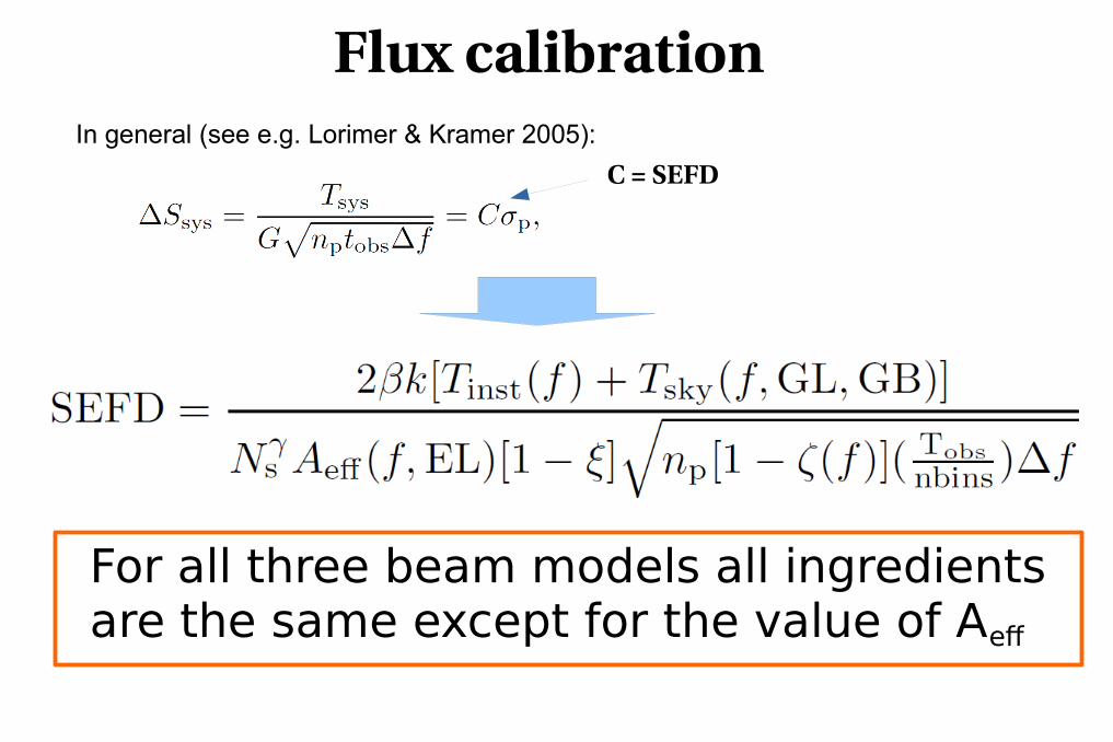
In general (see e.g. Lorimer & Kramer 2005):

Contributing factors

► Δf / f ~ 0.5 (huge)C = SEFDLOFAR

► Beam shape has strong dependence on AZ, EL, and frequency, and thus the gain, G► Gain(f) ≠ const► Tsys = Tsky + Tinst► Tsky(f) ~ f -2.55

► Tinst(f) ≠ const► Tsrc(f) ≠ const (ignore for now)

+► Broken tiles (~5%)► Coherence scaling S/N ~ N0.85, N — number of 48-tile stations► Radio frequency interference (RFI), on average 25-30% (MSP data, 1 ch/sub,

normally — much less)

Flux calibration In general (see e.g. Lorimer & Kramer 2005):

C = SEFD

β — digitization factor = 1 GL, GB — Galactic longitude and latitudeγ — coherence factor ≈ 0.85N

s — number of stations used

np — number of polarizations (2)

Aeff

— effective area of a 48-tile station

ξ — average fraction of bad/flagged dipoles/tilesζ — RFI fractionnbins — number of bins in the profileT

obs — observation length (s)

Δf — frequency channel width (Hz)

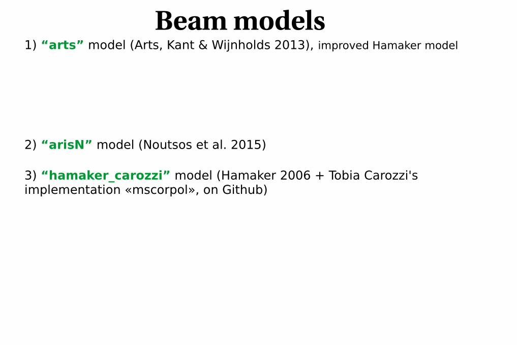
Beam models 1) “arts” model (Arts, Kant & Wijnholds 2013), improved Hamaker model

2) “arisN” model (Noutsos et al. 2015)

3) “hamaker_carozzi” model (Hamaker 2006 + Tobia Carozzi's implementation «mscorpol», on Github)

Beam models 

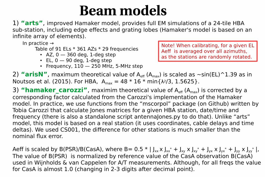
In practice → Table of 91 ELs * 361 AZs * 29 frequencies

● AZ, 0 — 360 deg, 1-deg step● EL, 0 — 90 deg, 1-deg step● Frequency, 110 — 250 MHz, 5-MHz step

Note! When calibrating, for a given ELAeff is averaged over all azimuths, as the stations are randomly rotated.

1) “arts”, improved Hamaker model, provides full EM simulations of a 24-tile HBA sub-station, including edge effects and grating lobes (Hamaker's model is based on an infinite array of elements).

2) “arisN”, maximum theoretical value of Aeff (Amax) is scaled as ~sin(EL)^1.39 as in Noutsos et al. (2015). For HBA, Amax = 48 * 16 * min{λ2/3, 1.5625}.

3) “hamaker_carozzi”, maximim theoretical value of Aeff (Amax) is corrected by a corresponding factor calculated from the Carozzi's implementation of the Hamaker model. In practice, we use functions from the “mscorpol” package (on Github) written by Tobia Carozzi that calculate Jones matrices for a given HBA station, date/time and frequency (there is also a standalone script antennaJones.py to do that). Unlike “arts” model, this model is based on a real station (it uses coordinates, cable delays and time deltas). We used CS001, the difference for other stations is much smaller than the nominal flux error.

Aeff is scaled by B(PSR)/B(CasA), where B= 0.5 * | Jxx x Jxx* + Jxy x Jxy

* + Jyx x Jyx* + Jyy x Jyy

* |,The value of B(PSR) is normalized by reference value of the CasA observation B(CasA) used in Wijnholds & van Cappelen for A/T measurements. Although, for all freqs the value for CasA is almost 1.0 (changing in 2-3 digits after decimal point).

Flux calibration In general (see e.g. Lorimer & Kramer 2005):

C = SEFD

For all three beam models all ingredients are the same except for the value of Aeff

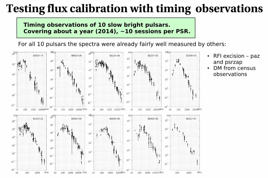
For all 10 pulsars the spectra were already fairly well measured by others:

Timing observations of 10 slow bright pulsars. Covering about a year (2014), ~10 sessions per PSR.

● RFI excision – paz and psrzap

● DM from census observations

Testing flux calibration with timing  observations

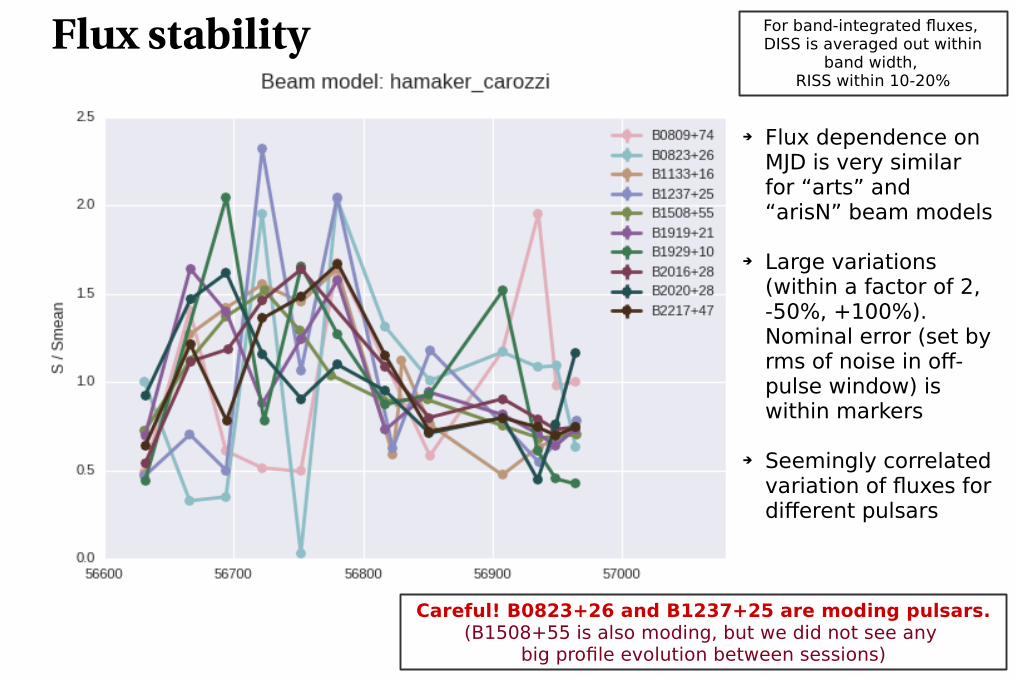
Flux stability

Careful! B0823+26 and B1237+25 are moding pulsars.(B1508+55 is also moding, but we did not see any

big profile evolution between sessions)

➔ Flux dependence on MJD is very similar for “arts” and “arisN” beam models

➔ Large variations (within a factor of 2, -50%, +100%). Nominal error (set by rms of noise in off-pulse window) is within markers

➔ Seemingly correlated variation of fluxes for different pulsars

For band-integrated fluxes, DISS is averaged out within

band width, RISS within 10-20%

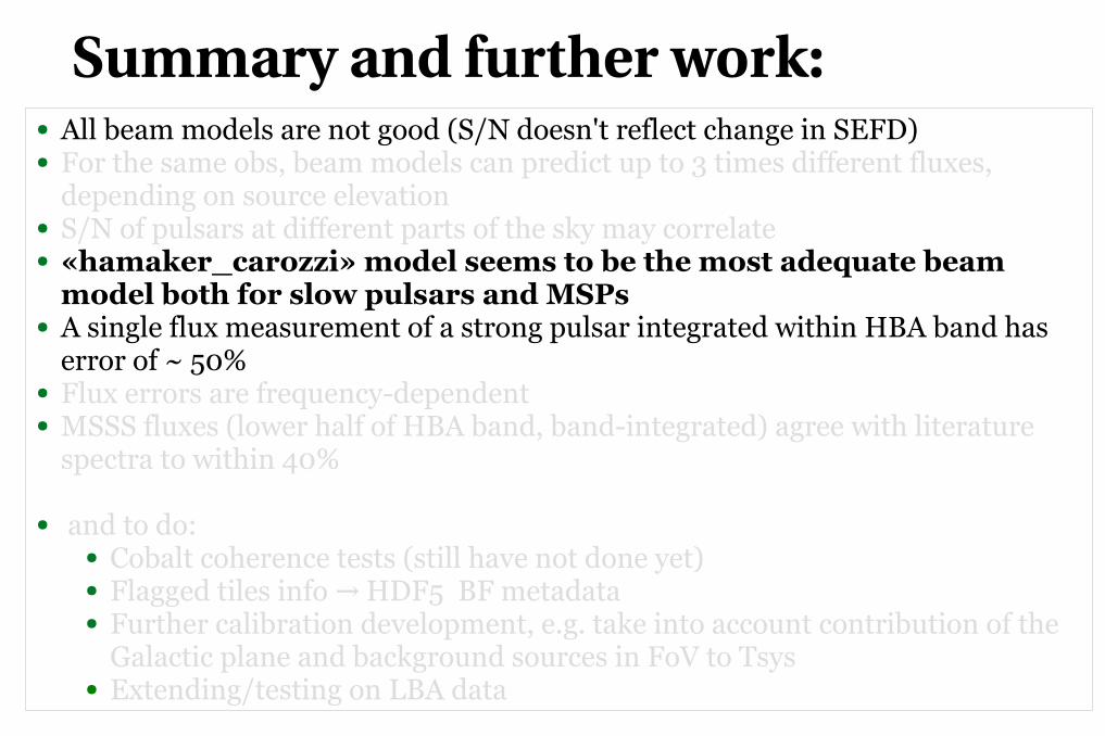
Summary and further work:● All beam models are not good (S/N doesn't reflect change in SEFD)● For the same obs, beam models can predict up to 3 times different fluxes,

depending on source elevation● S/N of pulsars at different parts of the sky may correlate● «hamaker_carozzi» model seems to be the most adequate beam

model both for slow pulsars and MSPs● A single flux measurement of a strong pulsar integrated within HBA band has

error of ~ 50%● Flux errors are frequency-dependent● MSSS fluxes (lower half of HBA band, band-integrated) agree with literature

spectra to within 40%

● and to do: ● Cobalt coherence tests (still have not done yet)● Flagged tiles info HDF5 BF metadata→● Further calibration development, e.g. take into account contribution of the

Galactic plane and background sources in FoV to Tsys● Extending/testing on LBA data

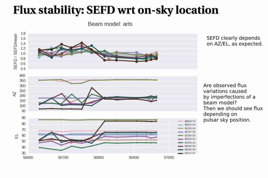
Flux stability: SEFD wrt on­sky locationFlux stability: SEFD wrt on­sky location

SEFD clearly dependson AZ/EL, as expected.

Are observed flux variations causedby imperfections of a beam model?Then we should see flux depending onpulsar sky position.

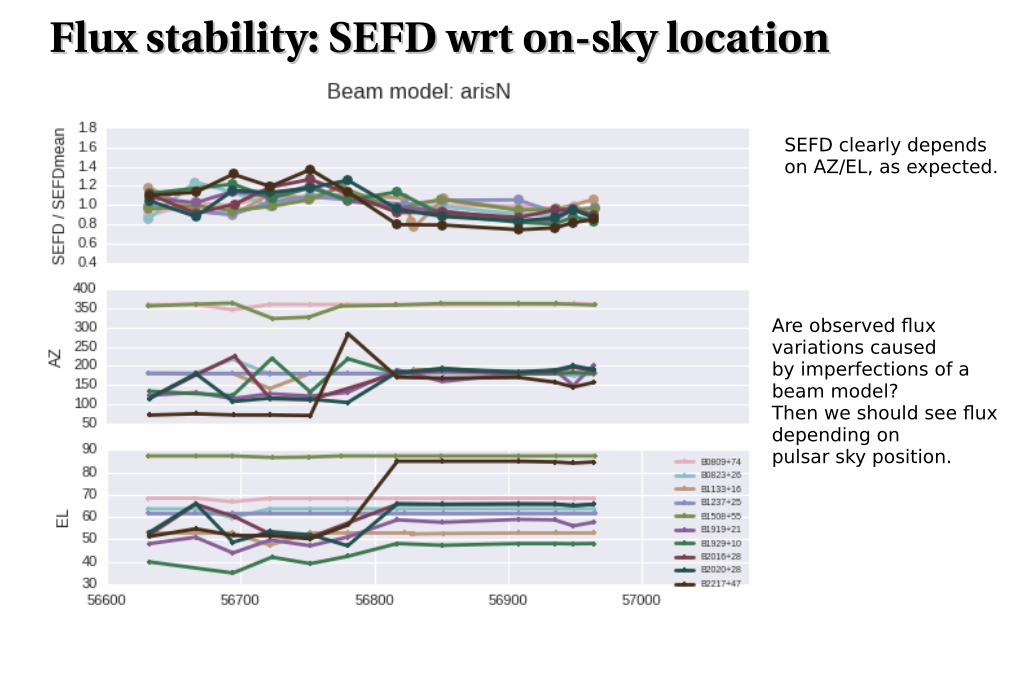
Flux stability: SEFD wrt on­sky locationFlux stability: SEFD wrt on­sky location

Are observed flux variations causedby imperfections of a beam model?Then we should see flux depending onpulsar sky position.

SEFD clearly dependson AZ/EL, as expected.

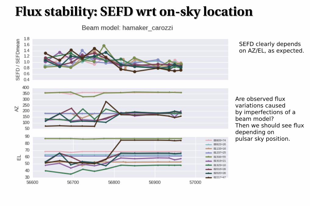
Flux stability: SEFD wrt on­sky locationFlux stability: SEFD wrt on­sky location

SEFD clearly dependson AZ/EL, as expected.

Are observed flux variations causedby imperfections of a beam model?Then we should see flux depending onpulsar sky position.

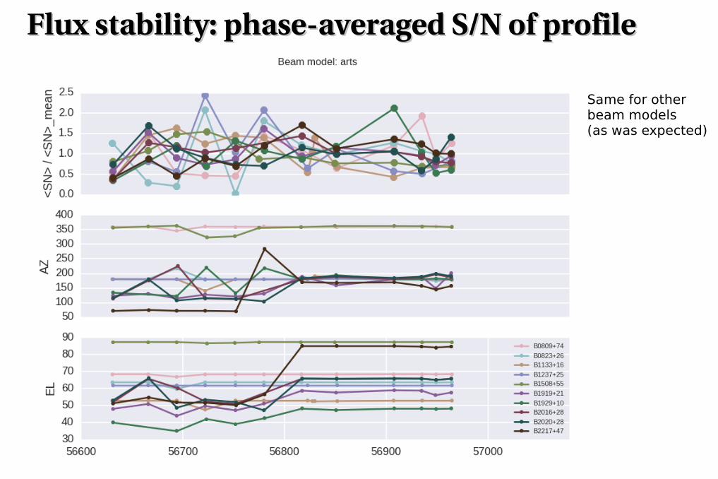
Flux stability: phase­averaged S/N of profileFlux stability: phase­averaged S/N of profile

Same for otherbeam models(as was expected)

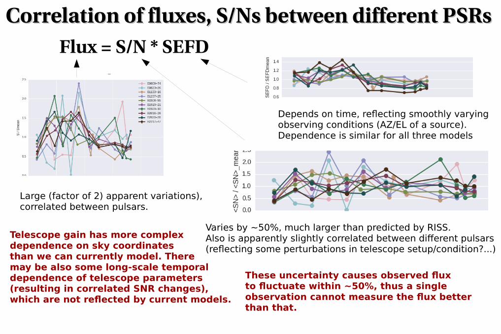
Correlation of fluxes, S/Ns between different PSRsCorrelation of fluxes, S/Ns between different PSRsFlux = S/N * SEFD

Varies by ~50%, much larger than predicted by RISS.Also is apparently slightly correlated between different pulsars(reflecting some perturbations in telescope setup/condition?...)

Depends on time, reflecting smoothly varying observing conditions (AZ/EL of a source). Dependence is similar for all three models

Large (factor of 2) apparent variations),correlated between pulsars.

Telescope gain has more complexdependence on sky coordinatesthan we can currently model. There may be also some long-scale temporal dependence of telescope parameters (resulting in correlated SNR changes),which are not reflected by current models.

These uncertainty causes observed fluxto fluctuate within ~50%, thus a single observation cannot measure the flux better than that.

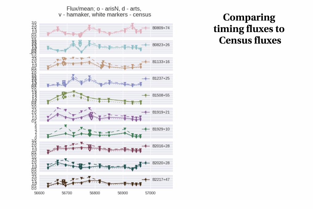
Comparing timing fluxes to 

Census fluxes

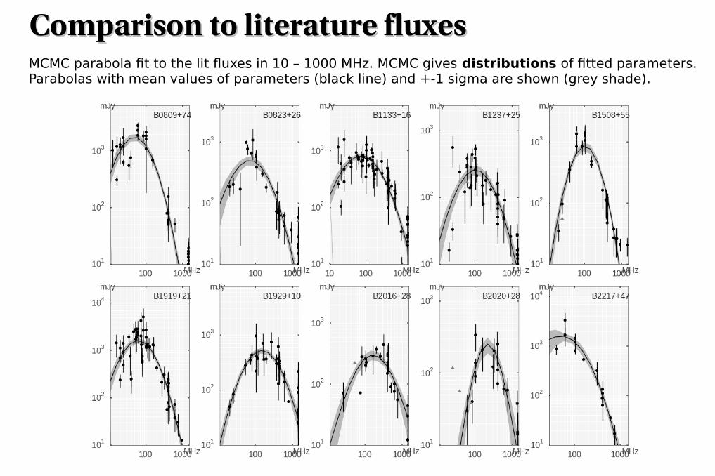
Comparison to literature fluxes Comparison to literature fluxes MCMC parabola fit to the lit fluxes in 10 – 1000 MHz. MCMC gives distributions of fitted parameters. Parabolas with mean values of parameters (black line) and +-1 sigma are shown (grey shade).

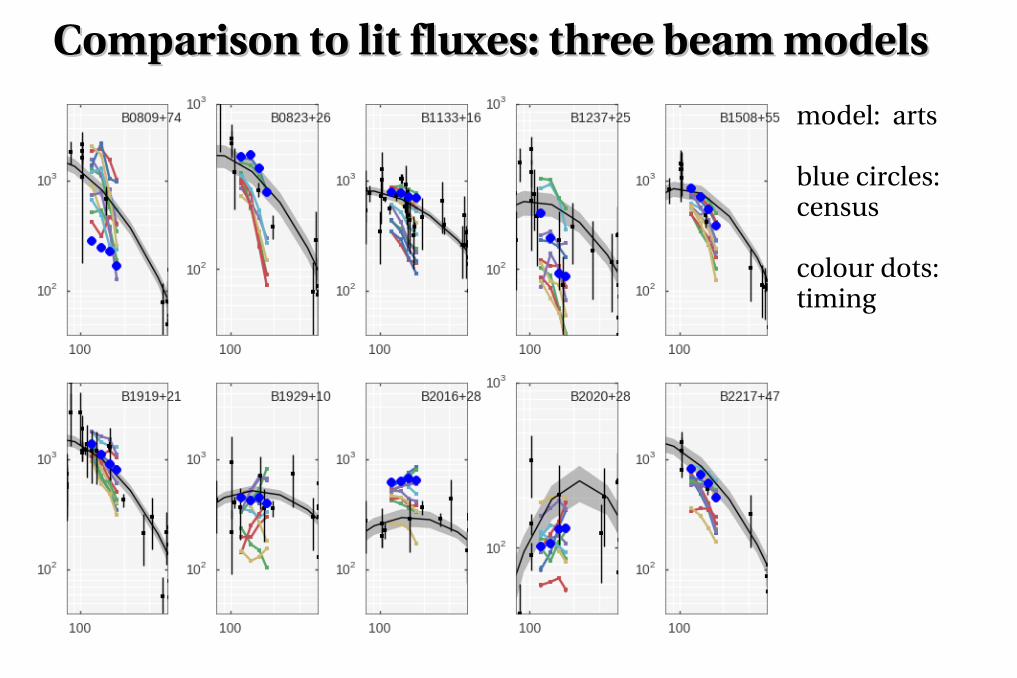
Comparison to lit fluxes: three beam models Comparison to lit fluxes: three beam models 

model:  arts

blue circles: census

colour dots:timing

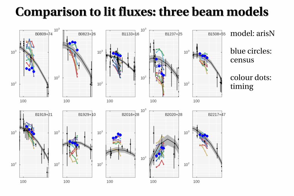
Comparison to lit fluxes: three beam models Comparison to lit fluxes: three beam models 

model: arisN

blue circles: census

colour dots:timing

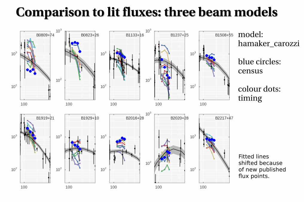
Fitted lines shifted because of new publishedflux points.

Comparison to lit fluxes: three beam models Comparison to lit fluxes: three beam models 

model: hamaker_carozzi

blue circles: census

colour dots:timing

Error distributionError distributionFor timing pulsars we can measure the distribution of K = Sr/So, the ratio ofthe real pulsar flux Sr to observed flux So. 

This distribution reflects our uncertainty about telescope parameters as well as ISM influence.

We assume that p(K) is the same for all pulsars regardless of their brightness.

Then, for a single So measurement the probability of getting Sr=Sr (some fixed value) is p(Sr=Sr | So=So) = p(Sr=K*So | So) = p(K).

For the histogram of K = Sr/So, we did not use a single value for Sr, but ~200 values weighted withprobabilities from MCMC fit.

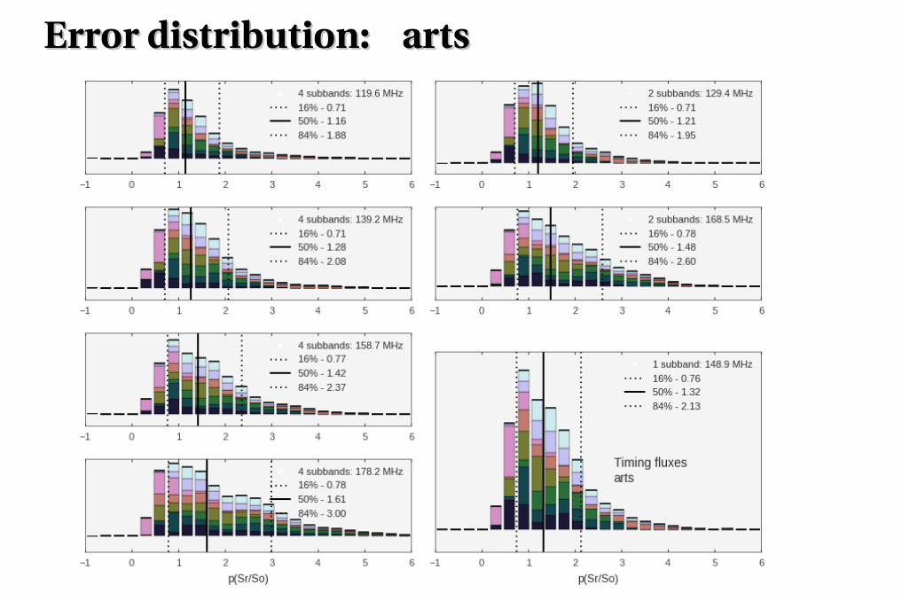
Error distribution:    arts Error distribution:    arts 

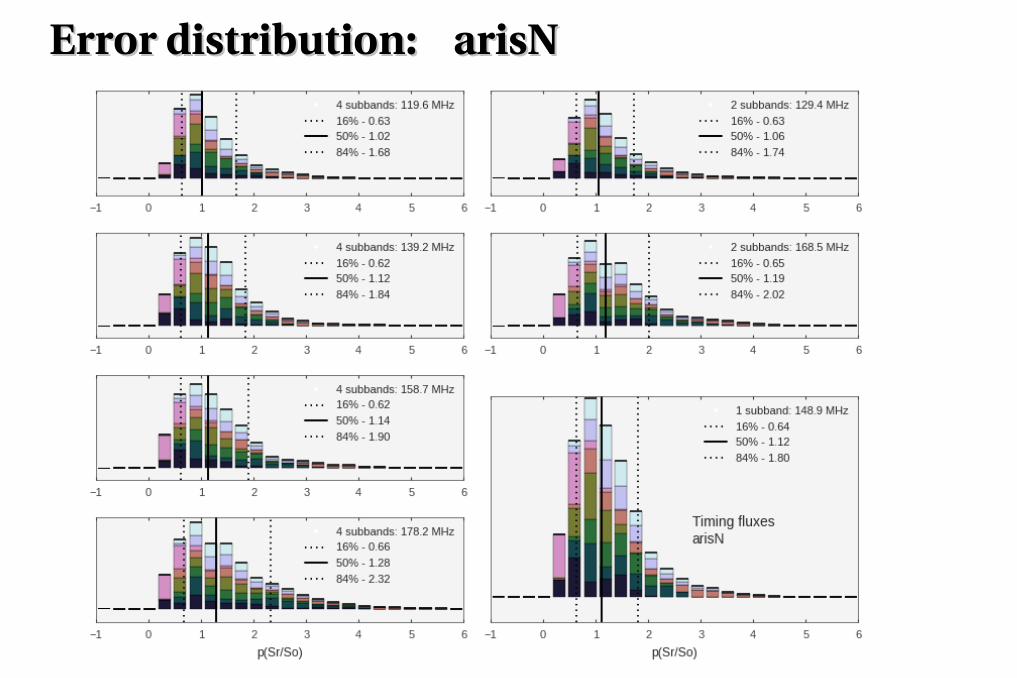
Error distribution:    arisN Error distribution:    arisN 

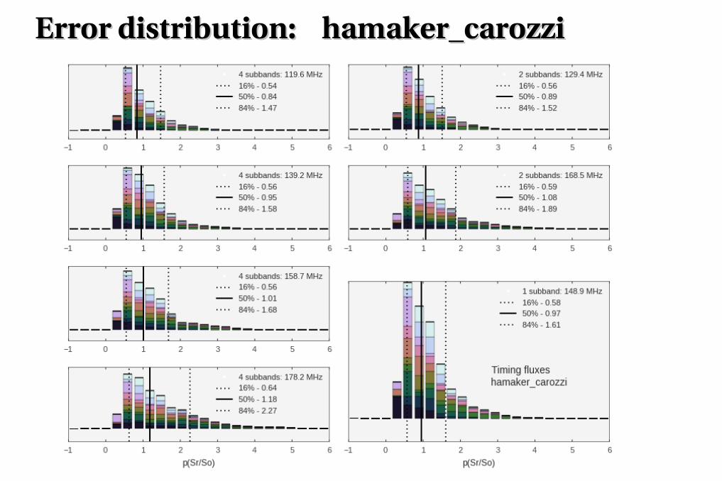
Error distribution:    hamaker_carozzi Error distribution:    hamaker_carozzi 

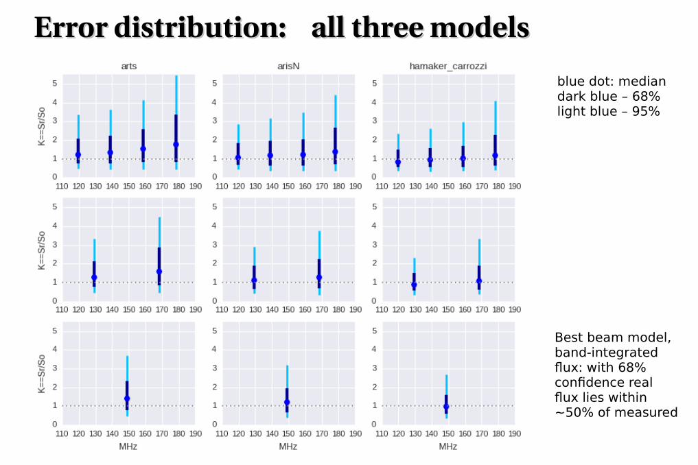
blue dot: mediandark blue – 68%light blue – 95%

Best beam model,band-integratedflux: with 68%confidence realflux lies within~50% of measured

Error distribution:    all three modelsError distribution:    all three models

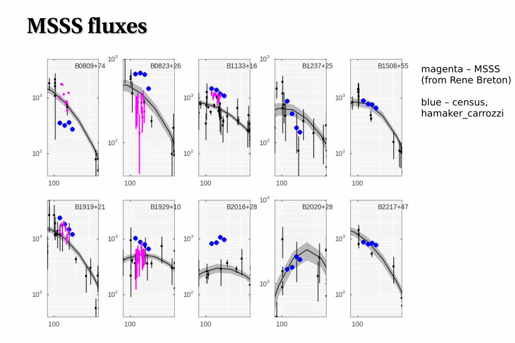
MSSS fluxesMSSS fluxes

magenta – MSSS(from Rene Breton)

blue – census,hamaker_carrozzi

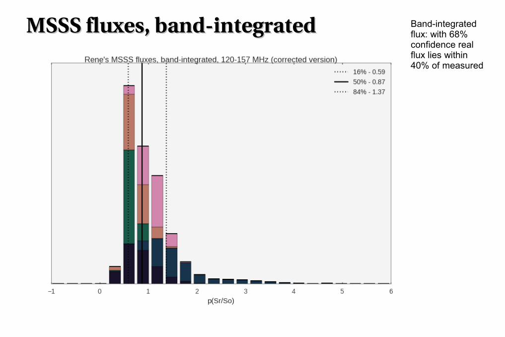
MSSS fluxes, band­integratedMSSS fluxes, band­integrated Band-integratedflux: with 68%confidence realflux lies within40% of measured

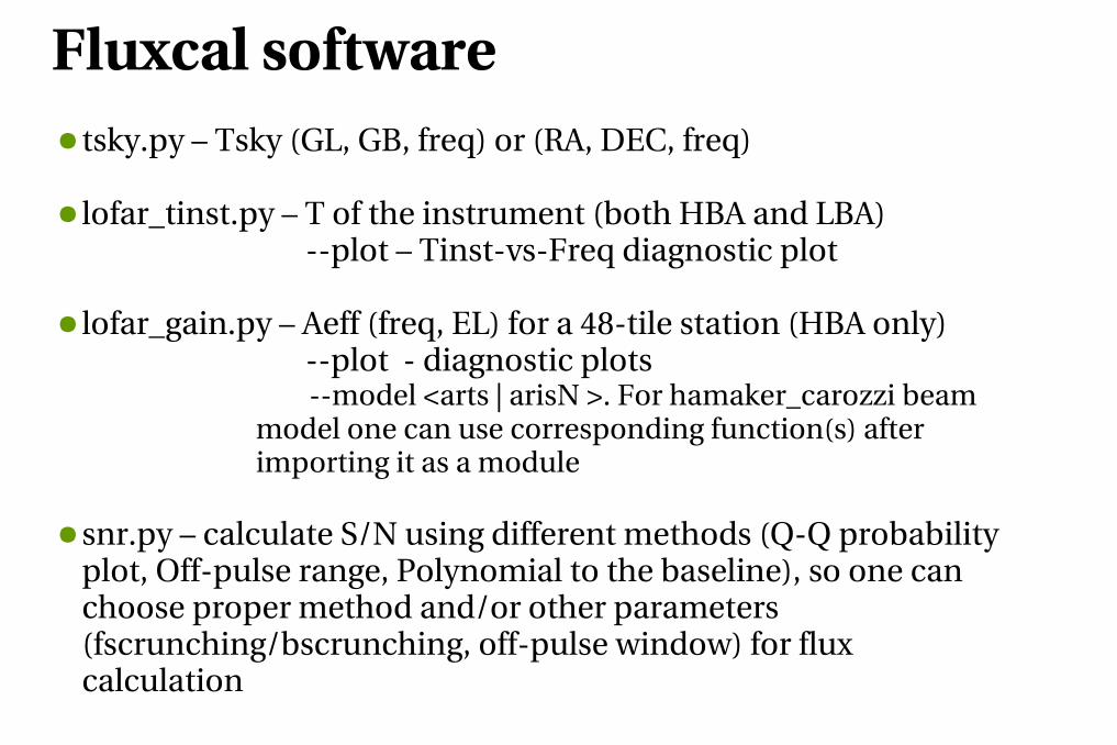
●tsky.py – Tsky (GL, GB, freq) or (RA, DEC, freq)

● lofar_tinst.py – T of the instrument (both HBA and LBA)­­plot – Tinst­vs­Freq diagnostic plot

● lofar_gain.py – Aeff (freq, EL) for a 48­tile station (HBA only)­­plot  ­ diagnostic plots

        ­­model <arts | arisN >. For hamaker_carozzi beam model one can use corresponding function(s) after importing it as a module 

●snr.py – calculate S/N using different methods (Q­Q probability plot, Off­pulse range, Polynomial to the baseline), so one can choose proper method and/or other parameters (fscrunching/bscrunching, off­pulse window) for flux calculation 

Fluxcal software

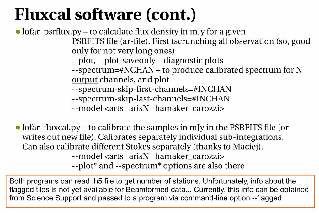
● lofar_psrflux.py – to calculate flux density in mJy for a givenPSRFITS file (ar­file). First tscrunching all observation (so, good only for not very long ones)­­plot, ­­plot­saveonly – diagnostic plots­­spectrum=#NCHAN – to produce calibrated spectrum for N output channels, and plot­­spectrum­skip­first­channels=#INCHAN­­spectrum­skip­last­channels=#INCHAN­­model <arts | arisN | hamaker_carozzi>

● lofar_fluxcal.py – to calibrate the samples in mJy in the PSRFITS file (orwrites out new file). Calibrates separately individual sub­integrations.Can also calibrate different Stokes separately (thanks to Maciej). 

­­model <arts | arisN | hamaker_carozzi>­­plot* and ­­spectrum* options are also there

Both programs can read .h5 file to get number of stations. Unfortunately, info about the flagged tiles is not yet available for Beamformed data... Currently, this info can be obtained from Science Support and passed to a program via command-line option --flagged

Fluxcal software (cont.)

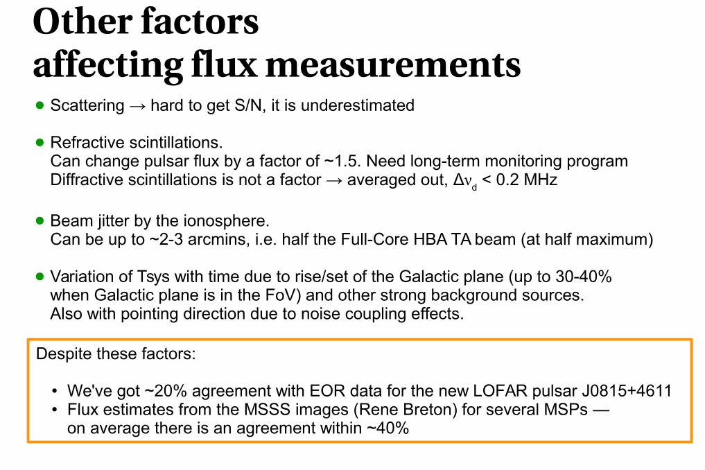
Other factors affecting flux measurements● Scattering → hard to get S/N, it is underestimated

● Refractive scintillations. Can change pulsar flux by a factor of ~1.5. Need long-term monitoring programDiffractive scintillations is not a factor → averaged out, Δν

d < 0.2 MHz

● Beam jitter by the ionosphere.Can be up to ~2-3 arcmins, i.e. half the Full-Core HBA TA beam (at half maximum)

● Variation of Tsys with time due to rise/set of the Galactic plane (up to 30-40% when Galactic plane is in the FoV) and other strong background sources.Also with pointing direction due to noise coupling effects.

Despite these factors:

● We've got ~20% agreement with EOR data for the new LOFAR pulsar J0815+4611● Flux estimates from the MSSS images (Rene Breton) for several MSPs —

on average there is an agreement within ~40%

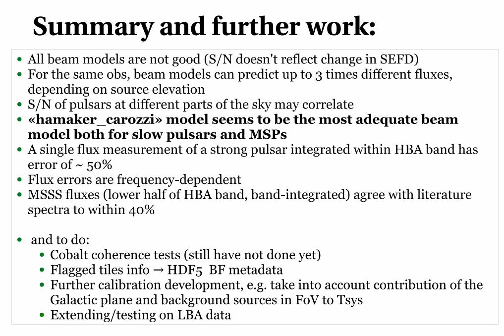
Summary and further work:● All beam models are not good (S/N doesn't reflect change in SEFD)● For the same obs, beam models can predict up to 3 times different fluxes,

depending on source elevation● S/N of pulsars at different parts of the sky may correlate● «hamaker_carozzi» model seems to be the most adequate beam

model both for slow pulsars and MSPs● A single flux measurement of a strong pulsar integrated within HBA band has

error of ~ 50%● Flux errors are frequency-dependent● MSSS fluxes (lower half of HBA band, band-integrated) agree with literature

spectra to within 40%

● and to do: ● Cobalt coherence tests (still have not done yet)● Flagged tiles info HDF5 BF metadata→● Further calibration development, e.g. take into account contribution of the

Galactic plane and background sources in FoV to Tsys● Extending/testing on LBA data

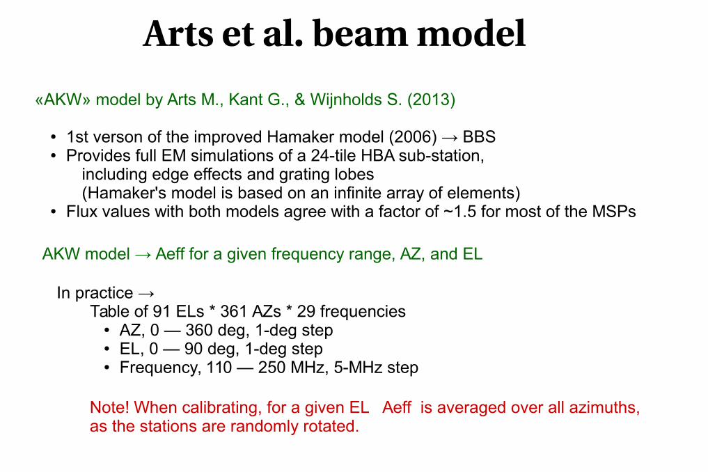
Arts et al. beam model 

«AKW» model by Arts M., Kant G., & Wijnholds S. (2013)

● 1st verson of the improved Hamaker model (2006) → BBS● Provides full EM simulations of a 24-tile HBA sub-station,

including edge effects and grating lobes(Hamaker's model is based on an infinite array of elements)

● Flux values with both models agree with a factor of ~1.5 for most of the MSPs

AKW model → Aeff for a given frequency range, AZ, and EL

In practice → Table of 91 ELs * 361 AZs * 29 frequencies

● AZ, 0 — 360 deg, 1-deg step● EL, 0 — 90 deg, 1-deg step● Frequency, 110 — 250 MHz, 5-MHz step

Note! When calibrating, for a given EL Aeff is averaged over all azimuths, as the stations are randomly rotated.

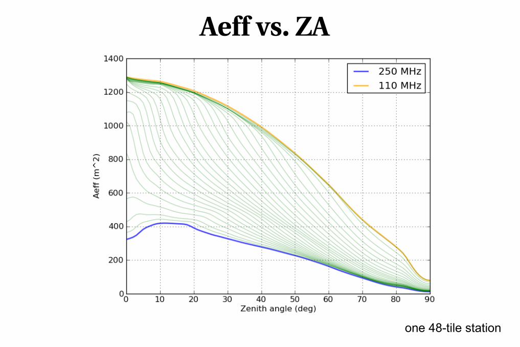
Aeff vs. ZA

one 48-tile station

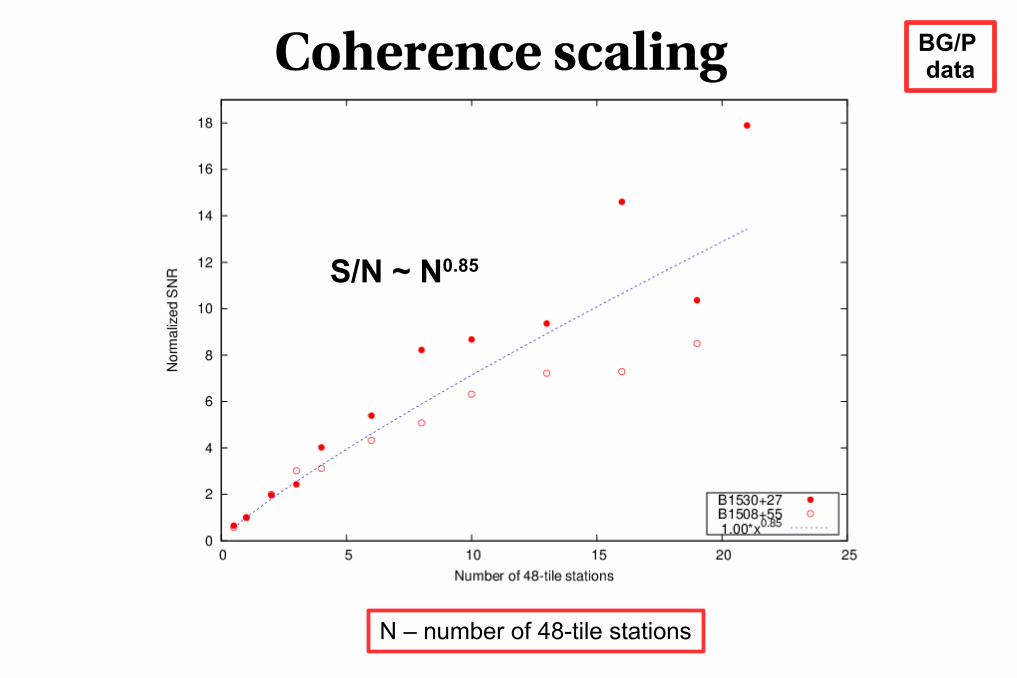
BG/P data

N – number of 48-tile stations

S/N ~ N0.85

Coherence scaling 

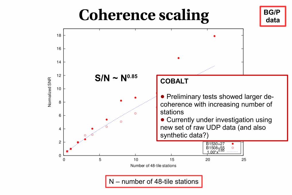
BG/P data

N – number of 48-tile stations

S/N ~ N0.85

Coherence scaling 

COBALT

● Preliminary tests showed larger de-coherence with increasing number of stations● Currently under investigation using new set of raw UDP data (and also synthetic data?)

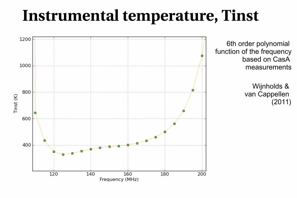
Instrumental temperature, Tinst

Wijnholds & van Cappellen

(2011)

6th order polynomial function of the frequency

based on CasA measurements

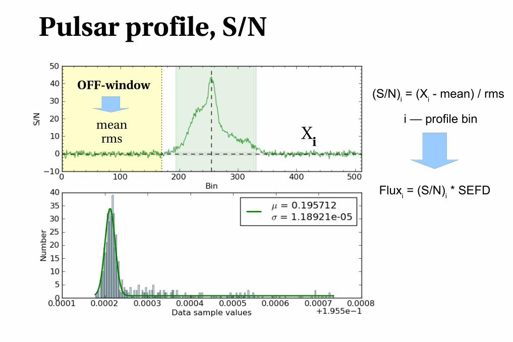
Pulsar profile, S/N

OFF­window

Ximeanrms

(S/N)i = (X

i - mean) / rms

i — profile bin

Fluxi = (S/N)

i * SEFD