Lie Algebra - Fermilab

Lecture 7:

Lie Algebra

Yunhai Cai SLAC National Accelerator Laboratory

June 14, 2017

USPAS June 2017, Lisle, IL, USA

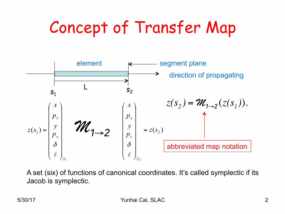
Concept of Transfer Map

5/30/17 Yunhai Cai, SLAC 2

s1 s2

element

L

direction of propagating

segment plane

M1→2

1s

y

x

1 pypx

sz

⎟⎟⎟⎟⎟⎟⎟

⎠

⎞

⎜⎜⎜⎜⎜⎜⎜

⎝

⎛

=

ℓδ

)( )( 2

s

y

x

szpypx

2

=

⎟⎟⎟⎟⎟⎟⎟

⎠

⎞

⎜⎜⎜⎜⎜⎜⎜

⎝

⎛

ℓδ

A set (six) of functions of canonical coordinates. It’s called symplectic if its Jacob is symplectic.

z(s2 ) = M1→2 (z(s1)).

abbreviated map notation

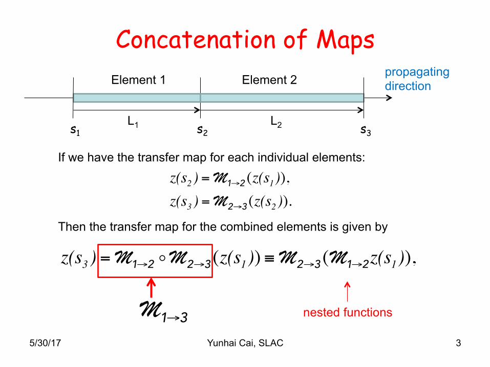
Concatenation of Maps


s2

Element 1

L1 s1 s3 L2

Element 2 propagating direction

z(s2 ) = M1→2 (z(s1)),z(s3 ) = M2→3 (z(s2 )).

If we have the transfer map for each individual elements:

z(s3 ) = M1→2 !M2→3 (z(s1)) ≡ M2→3 (M1→2z(s1)),

Then the transfer map for the combined elements is given by

nested functions M1→3

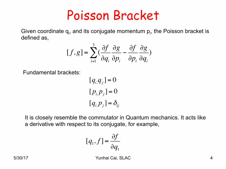
Poisson Bracket


[ f ,g]= ( ∂f∂qii=1

3

∑ ∂g∂pi

−∂f∂pi

∂g∂qi)

Given coordinate qi, and its conjugate momentum pi, the Poisson bracket is defined as,

Fundamental brackets: [qi,qj ]= 0[pi,pj ]= 0[qi,pj ]= δij

It is closely resemble the commutator in Quantum mechanics. It acts like a derivative with respect to its conjugate, for example,

[q1, f ]=∂f∂q1

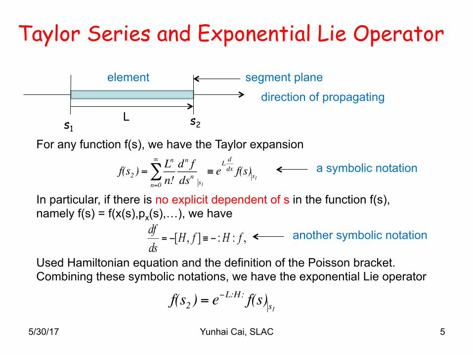
Taylor Series and Exponential Lie Operator


For any function f(s), we have the Taylor expansion

s1 s2

element

L

a symbolic notation


segment plane

In particular, if there is no explicit dependent of s in the function f(s), namely f(s) = f(x(s),px(s),…), we have

,::],[ fHfHdsdf

−≡−=

Used Hamiltonian equation and the definition of the Poisson bracket. Combining these symbolic notations, we have the exponential Lie operator

another symbolic notation

f(s2 ) =Ln

n!n=0

∞

∑ dn fdsn s1

≡ eL ddx f(s)s1

f(s2 ) = e−L:H: f(s)s1

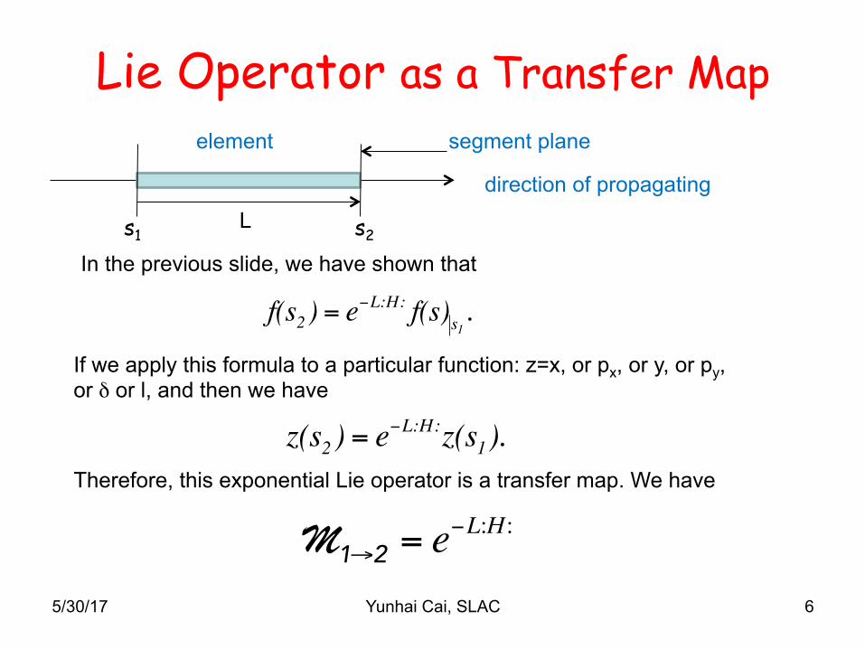
Lie Operator as a Transfer Map


f(s2 ) = e−L:H: f(s)s1.

s1 s2

element

L


segment plane

In the previous slide, we have shown that

If we apply this formula to a particular function: z=x, or px, or y, or py, or δ or l, and then we have

z(s2 ) = e−L:H:z(s1).

Therefore, this exponential Lie operator is a transfer map. We have

M1→2 = e−L:H :

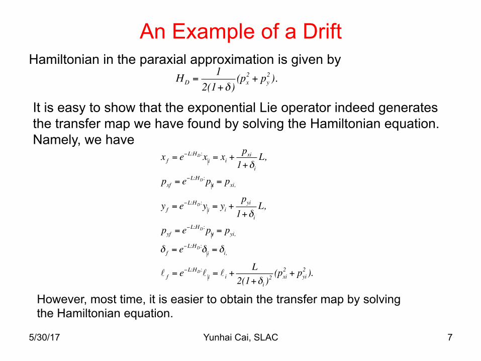
An Example of a Drift

HD =1

2(1+δ)(px

2 + py2 ).

Hamiltonian in the paraxial approximation is given by

x f = e−L:HD:xi = xi +

pxi1+δi

L,

pxf = e−L:HD:pxi = pxi,

y f = e−L:HD:yi = yi +

pyi1+δi

L,

pyf = e−L:HD:pyi = pyi,

δ f = e−L:HD:δ i = δi,

ℓ f = e−L:HD:ℓ i = ℓ i +

L2(1+δi )

2 (pxi2 + pyi

2 ).

It is easy to show that the exponential Lie operator indeed generates the transfer map we have found by solving the Hamiltonian equation. Namely, we have


However, most time, it is easier to obtain the transfer map by solving the Hamiltonian equation.

Lie Operators and Map Concatenation


s2

H1

L1 s1 s3 L2

H2

It is obvious that

f(s+ L) = e−L:H: f(x, px ,...) = f(e−L:H:x,e−L:H: px ,...) = f(x(s+ L), px (s+ L),...)

obviously true

just shown

just shown

The Lie operator acts only on the arguments of function . This precisely the definition of the map concatenation we introduced early. So we have

M1→3 = M1→2 !M2→3 = e−L1:H1:e−L2:H2:.

propagating direction

The dot is removed because Lie operator automatically has the property.

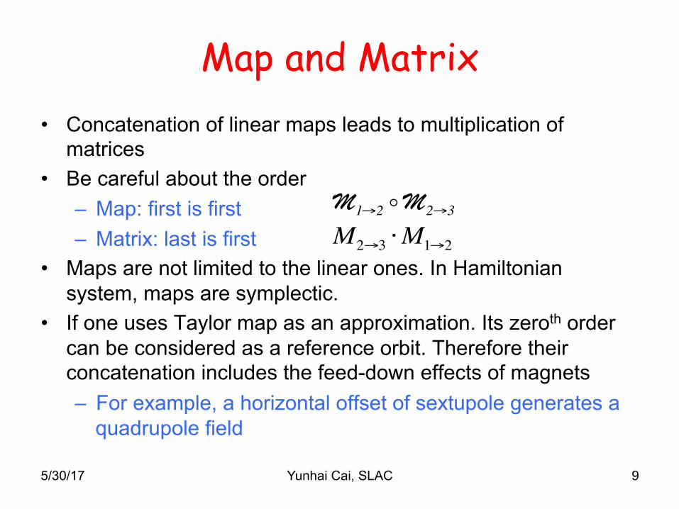
Map and Matrix •  Concatenation of linear maps leads to multiplication of

matrices •  Be careful about the order

–  Map: first is first –  Matrix: last is first

•  Maps are not limited to the linear ones. In Hamiltonian system, maps are symplectic.

•  If one uses Taylor map as an approximation. Its zeroth order can be considered as a reference orbit. Therefore their concatenation includes the feed-down effects of magnets –  For example, a horizontal offset of sextupole generates a

quadrupole field


M1→2 !M2→3

M2→3 ⋅M1→2

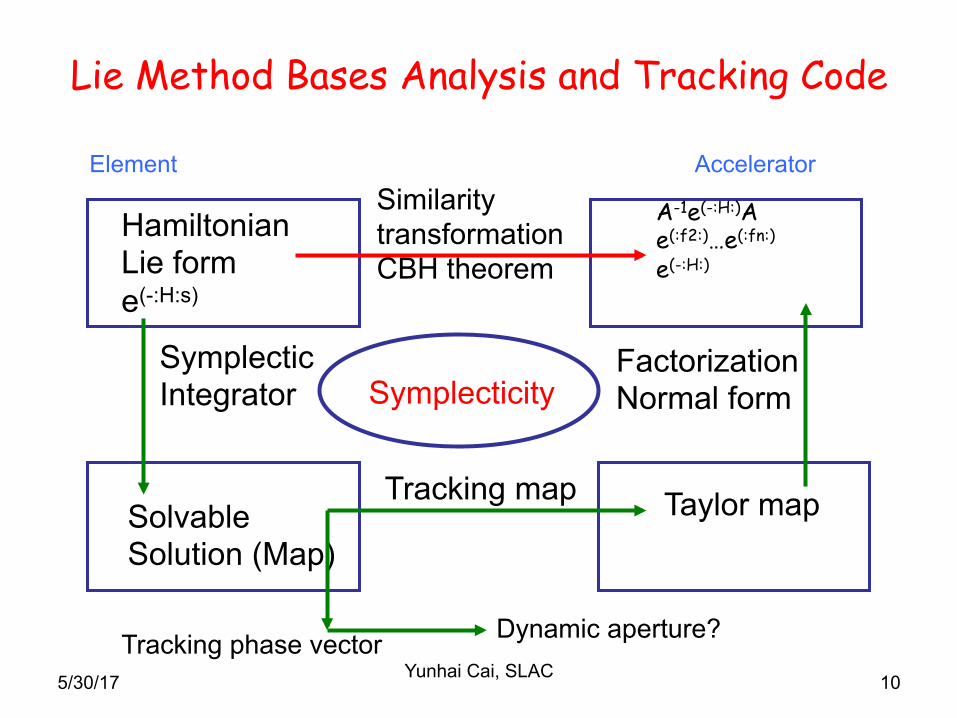
Lie Method Bases Analysis and Tracking Code

Hamiltonian Lie form e(-:H:s)

Element Accelerator

Solvable Solution (Map)

Symplectic Integrator

Tracking map Taylor map

Similarity transformation CBH theorem

Tracking phase vector Dynamic aperture?

Factorization Normal form Symplecticity

A-1e(-:H:)A e(:f2:)…e(:fn:)

e(-:H:)

10 Yunhai Cai, SLAC 5/30/17

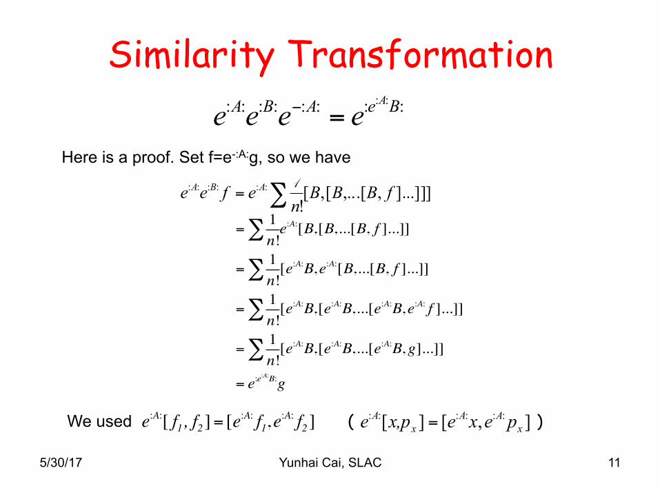
Similarity Transformation


:::::::: :: BeABA A

eeee =−

Here is a proof. Set f=e-:A:g, so we have

]...]]],,...[[,[!

:::::: fBBBn

efee ABA ∑=1

=1n!∑ e:A:[B,[B,...[B, f ]...]]

=1n!∑ [e:A:B,e:A:[B,...[B, f ]...]]

=1n!∑ [e:A:B,[e:A:B,...[e:A:B,e:A: f ]...]]

=1n!∑ [e:A:B,[e:A:B,...[e:A:B,g]...]]

= e:e:A:B:g

We used e:A:[ f1, f2 ]= [e:A: f1,e

:A: f2 ] ],[][ ::::::x

AAx

A pexex,pe =( )

The Cambell-Baker-Hausdorf (CBH) Theorem


:...],[::::: +++=

BA21BABA eee

The bracket notes the Poisson bracket. This theorem can be shown easily using the definition of the exponential Lie operator and the Jacob identity for the Poisson brackets:

To combine two exponential Lie operators, we have

0[C,[A,B]][B,[C,A]][A,[B,C]] =++

In general, it should be considered as a part of perturbation theory. It is good when A and B are small.

:::::: BABA eee +=This a necessary condition for the exponential Lie operator being a transfer map of the element that can be described by a Hamiltonian.

( actually, this is an exact result )

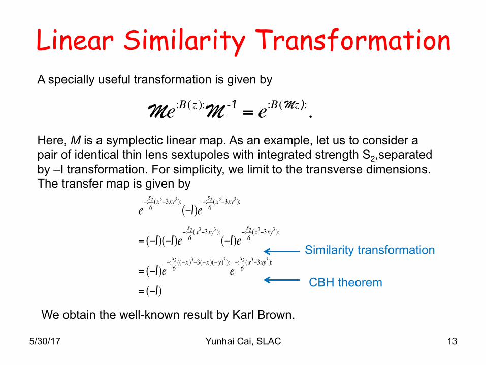
Linear Similarity Transformation


Me:B(z):M -1 = e:B(Mz ):.A specially useful transformation is given by

Here, M is a symplectic linear map. As an example, let us to consider a pair of identical thin lens sextupoles with integrated strength S2,separated by –I transformation. For simplicity, we limit to the transverse dimensions. The transfer map is given by

e−:s26(x3−3xy3 ):

(−I)e−:s26(x3−3xy3 ):

= (−I)(−I)e−:s26(x3−3xy3 ):

(−I)e−:s26(x3−3xy3 ):

= (−I)e−:s26((−x )3−3(−x )(−y)3 ):

e−:s26(x3−3xy3 ):

= (−I)

Similarity transformation

CBH theorem

We obtain the well-known result by Karl Brown.

Courant-Synder Invariance


ρG (x, px )∝ exp[−(γ xx

2 + 2αxxpx +βx px2 )

2λx]

It can be shown that the Lie operator:

is the transfer map of the Courant-Synder matrix:

Mx =cosµx +αx sinµx βx sinµx

−γ x sinµx cosµx −αx sinµx

⎛

⎝

⎜⎜

⎞

⎠

⎟⎟

Gaussian beam distribution:

exp[−µx :(γ xx

2 + 2αxxpx +βx px2 )

2] :

Calculate Nonlinear Hamiltonian


Consider a set of multipoles separated by linear maps. We can represent the nonlinear transfer map by

M0,1e−:V1(z)M1,2e

−:V2 (z)...Mn−1,ne−:Vn (z)Mn,n+1

= M0,1e−:V1 (z):M1,2e

−:V2 (z):...Mn−1,nMn,n+1Mn,n+1−1 e−:Vn (z):Mn,n+1

= M0,1e−:V1 (z):M1,2e

−:V2 (z):...Mn−1,nMn,n+1e−:Vn (Mn,n+1

−1 z):

= M0,n+1e−:V1(M1,n+1

−1 z):e−:V2 (M2,n+1−1 z):...e−:Vn (Mn,n+1

−1 z):

= M0,n+1e−:HNL:

similarity transformation

CBH theorem

We can use the similarity transformation and CBH theorem to obtain an effective Hamiltonian so that the transfer map consists of a linear map followed by an exponential Lie operator for the nonlinearity. It is very useful for understanding of the nonlinear effects and their compensation. Clearly, it is an approximation to a real accelerator.

z is the coordinates at the end.

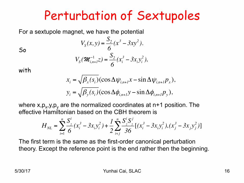
Perturbation of Sextupoles


xi = βx (si )(cosΔψi,n+1x − sinΔψi,n+1px ),

yi = βy (si )(cosΔφi,n+1y− sinΔφi,n+1py ),

VS (x, y) =S26(x3 − 3xy2).

For a sextupole magnet, we have the potential

So VS (Mi,n+1

−1 z) = S26(xi

3 − 3xiyi2 ),

with

where x,px,y,py are the normalized coordinates at n+1 position. The effective Hamiltonian based on the CBH theorem is

HNL =S

2

i

6(xi

3 − 3xiyi2 )

i=1

n

∑ +12

S2

i S2

j

36[(xi

3 − 3xiyi2 )

i< j

n

∑ , (x j3 − 3x jyj

2 )]

The first term is the same as the first-order canonical perturbation theory. Except the reference point is the end rather then the beginning.

Nonlinear Hamiltonian of Sextupoles


HNL =S

2

i

6(xi

3 − 3xiyi2 )

i=1

n

∑

+12

S2

i S2

j βx,iβx, ji< j

n

∑ {sin(Δφi,n+1 −Δφ j,n+1)βy,iβy, j xix j yiyj

+sin(Δψi,n+1 −Δψ j,n+1)(βx,i xi2 −βy,i yi

2 )(βx, j x j2 −βy, j y j

2 ) / 4}

The Poisson bracket can be evaluated, we have

We see that two sextupoles generate octopole like terms.

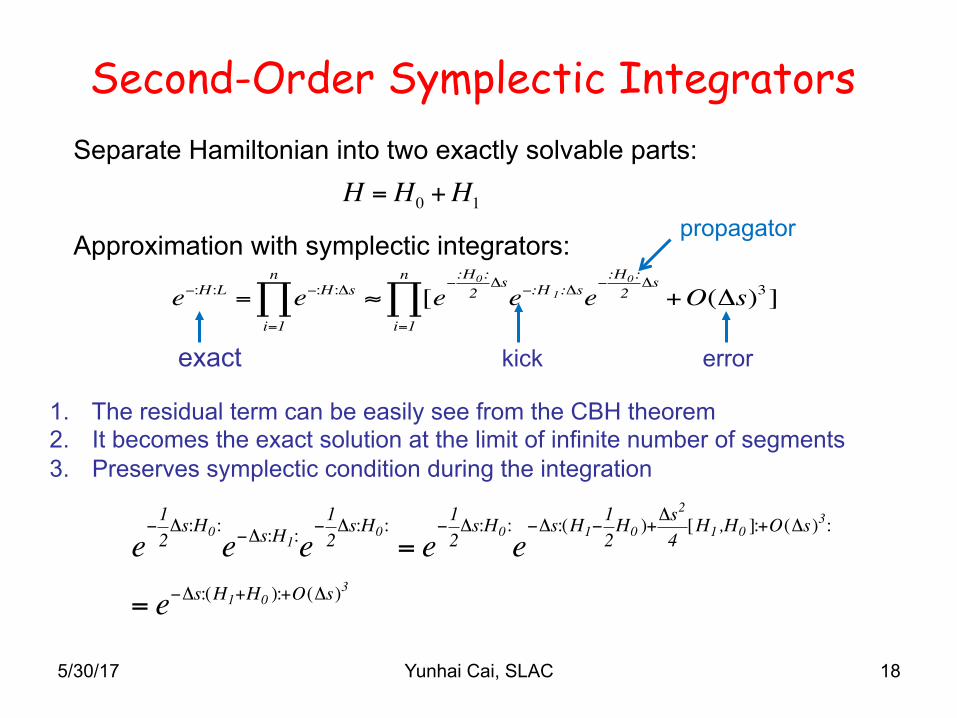
Second-Order Symplectic Integrators Separate Hamiltonian into two exactly solvable parts:

H = H0 +H1

Approximation with symplectic integrators:

exact kick error

1.  The residual term can be easily see from the CBH theorem 2.  It becomes the exact solution at the limit of infinite number of segments 3.  Preserves symplectic condition during the integration

propagator

e−:H :L = e−:H :Δsi=1

n

∏ ≈ [e−:H0:2

Δse−:H 1:Δse

−:H0:2

Δs+O(Δs)3

i=1

n

∏ ]

e−12Δs:H0:e−Δs:H1:e

−12Δs:H0:

= e−12Δs:H0:e

−Δs:(H1−12H0 )+

Δs2

4[H1,H0 ]:+O(Δs)

3:

= e−Δs:(H1+H0 ):+O(Δs)3


Summary •  Lie algebra is a powerful method for nonlinear analysis.

It is equivalent to the Hamiltonian perturbation •  Exponential Lie operator is a representation of the

transfer map –  Used to derive symplectic integrator –  Define transfer map of a beamline

•  Similarity transformation and the CBH theorem are two important tools in the Lie method –  Derive the nonlinear Hamiltonian

•  Courant-Synder invariance can be used as a quadratic polynomial for a Lie operator


References

1)  A.J. Dragt, J. Opt. Soc. An. 72, 372 (1982); A. Dragt et al. Ann. Rev. Nucl. Part. Sci. 38, 455 (1988).

2)  John Irwin, “The application of Lie algebra techniques to beam transport design,” SLAC-PUB-5315, Nucl. Instr. Meth. A 298, 460 (1990).

3)  Alex Chao, Lecture Notes, SLAC-PUB-9574, (2002). 4)  Yunhai Cai, Karl Bane, Robert Hettel, Yuri Nosochkov,

Min-Huey Wang, Michael Borland, “Ultimate storage ring based on fourth-order geometric achromats,” PRSTAB 15, 054002 (2012).


Acknowledgements Many thanks to Alex Chao, John Irwin, Etienne Forest, Yiton Yan form who I have learned over the years.

21 Yunhai Cai, SLAC 5/30/17

Lie Algebra - Fermilab

Documents

Transcript of Lie Algebra - Fermilab