Leon, R. Composite Connections Structural Engineering ...freeit.free.fr/Structure Engineering...

Leon, R. “Composite Connections”Structural Engineering HandbookEd. Chen Wai-FahBoca Raton: CRC Press LLC, 1999

Composite Connections

Roberto LeonSchool of Civil and EnvironmentalEngineering, Georgia Institute ofTechnology, Atlanta, GA

23.1 Introduction23.2 Connection Behavior Classification23.3 PR Composite Connections23.4 Moment-Rotation (M-θ) Curves23.5 Design of Composite Connections in Braced Frames23.6 Design for Unbraced FramesReferences

23.1 Introduction

The vast majority of steel buildings built today incorporate a floor system consisting of compositebeams, composite joists or trusses, stub girders, or some combination thereof [29]. Traditionallythe strength and stiffness of the floor slabs have only been used for the design of simply-supportedflexural members under gravity loads, i.e., for members bent in single curvature about the strong axisof the section. In this case the members are assumed to be pin-ended, the cross-section is assumed tobe prismatic, and the effective width of the slab is approximated by simple rules. These assumptionsallow for a member-by-member design procedure and considerably simplify the checks needed forstrength and serviceability limit states. Although most structural engineers recognize that there issome degree of continuity in the floor system because of the presence of reinforcement to controlcrack widths over column lines, this effect is considered difficult to quantify and thus ignored indesign.

The effect of the floor slabs has also been neglected when assessing the strength and stiffness offrames subjected to lateral loads for four principal reasons. First, it has been assumed that neglectingthe additional strength and stiffness provided by the floor slabs always results in a conservative design.Second, a sound methodology for determining the M-θ curves for these connections is a prerequisiteif their effect is going to be incorporated into the analysis. However, there is scant data availablein order to formulate reliable moment-rotation (M-θ) curves for composite connections, which falltypically into the partially restrained (PR) and partial strength (PS) category. Third, it is difficultto incorporate into the analysis the non-prismatic composite cross-section that results when themember is subjected to double curvature as would occur under lateral loads. Finally, the degree ofcomposite interaction in floor members that are part of lateral-load resisting systems in seismic areasis low, with most having only enough shear transfer capacity to satisfy diaphragm action.

Research during the past 10 years [25] and damage to steel frames during recent earthquakes [22]have pointed out, however, that there is a need to reevaluate the effect of composite action in modernframes. The latter are characterized by the use of few bents to resist lateral loads, with the ratioof number of gravity to moment-resisting columns often as high as 6 or more. In these cases the

c©1999 by CRC Press LLC

aggregate effect of many PR/PS connections can often add up to a significant portion of the lateralresistance of a frame. For example, many connections that were considered as pins in the analysis(i.e., connections to columns in the gravity load system) provided considerable lateral strength andstiffness to steel moment-resisting frames (MRFs) damaged during the Northridge earthquake. Inthese cases many of the fully restrained (FR) welded connections failed early in the load history,but the frames generally performed well. It has been speculated that the reason for the satisfactoryperformance was that the numerous PR/PS connections in the gravity load system were able toprovide the required resistance since the input base shear decreased as the structure softened. Inthese PR/PS connections, much of the additional capacity arises from the presence of the floor slabwhich provides a moment transfer mechanism not accounted for in design.

In this chapter general design considerations for a particular type of composite PR/PS connectionwill be given and illustrated with examples for connections in braced and unbraced frames. Infor-mation on design of other types of bolted and composite PR connections is given elsewhere [22],(Chapter 6 of [29]). The chapter begins with discussions of both the development of M-θ curves andthe effect of PR connections on frame analysis and design. A clear understanding of these two topicsis essential to the implementation of the design provisions that have been proposed for this type ofconstruction [26] and which will be illustrated herein.

23.2 Connection Behavior Classification

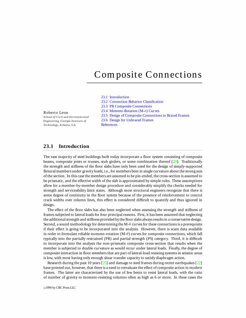
The first step in the design of a building frame, after the general topology, the external loads, thematerials, and preliminary sizes have been selected, is to carry out an analysis to determine memberforces and displacements. The results of this analysis depend strongly on the assumptions made inconstructing the structural model. Until recently most computer programs available to practicingengineers provided only two choices (rigid or pinned) for defining the connections stiffness. Inreality connections are very complex structural elements and their behavior is best characterized byM-θ curves such as those given in Figure 23.1 for typical steel connections to an A36 W24x55 beam(Mp,beam = 4824 kip-in.). In Figure 23.1, Mconn corresponds to the moment at the column face,while θconn corresponds to the total rotation of the connection and a portion of the beam generallytaken as equal to the beam depth. These curves are shown for illustrative purposes only, so that thedifferent connection types can be contrasted. For each of the connection types shown, the curves canbe shifted through a wide range by changing the connection details, i.e., the thickness of the anglesin the top and seat angle case.

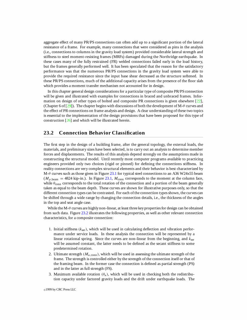
While the M-θ curves are highly non-linear, at least three key properties for design can be obtainedfrom such data. Figure 23.2 illustrates the following properties, as well as other relevant connectioncharacteristics, for a composite connection:

1. Initial stiffness (kser), which will be used in calculating deflection and vibration perfor-mance under service loads. In these analysis the connection will be represented by alinear rotational spring. Since the curves are non-linear from the beginning, and kser

will be assumed constant, the latter needs to be defined as the secant stiffness to somepredetermined rotation.

2. Ultimate strength (Mu,conn), which will be used in assessing the ultimate strength of theframe. The strength is controlled either by the strength of the connection itself or that ofthe framing beam. In the former case the connection is defined as partial strength (PS)and in the latter as full strength (FS).

3. Maximum available rotation (θu), which will be used in checking both the redistribu-tion capacity under factored gravity loads and the drift under earthquake loads. The


FIGURE 23.1: Typical moment-rotation curves for steel connections.

FIGURE 23.2: Definition of connection properties for PR connections.

required rotational capacity depends on the design assumptions and the redundancy ofthe structure.

It is often useful also to define a fourth quantity, the ductility (µ) of the connection. This is definedas the ratio of the ultimate rotation capacity (θu) to some nominal “yield” rotation (θy). It should beunderstood that the definition of θy is subjective and needs to account for the shape of the curve (i.e.,how sharp is the transition from the service to the yield level — the sharper the transition the morevalid the definition shown in Figure 23.2). In the design procedure to be discussed in this chapter,the initial stiffness, ultimate strength, maximum rotation, and ductility are properties that will needto be check by the structural engineer.


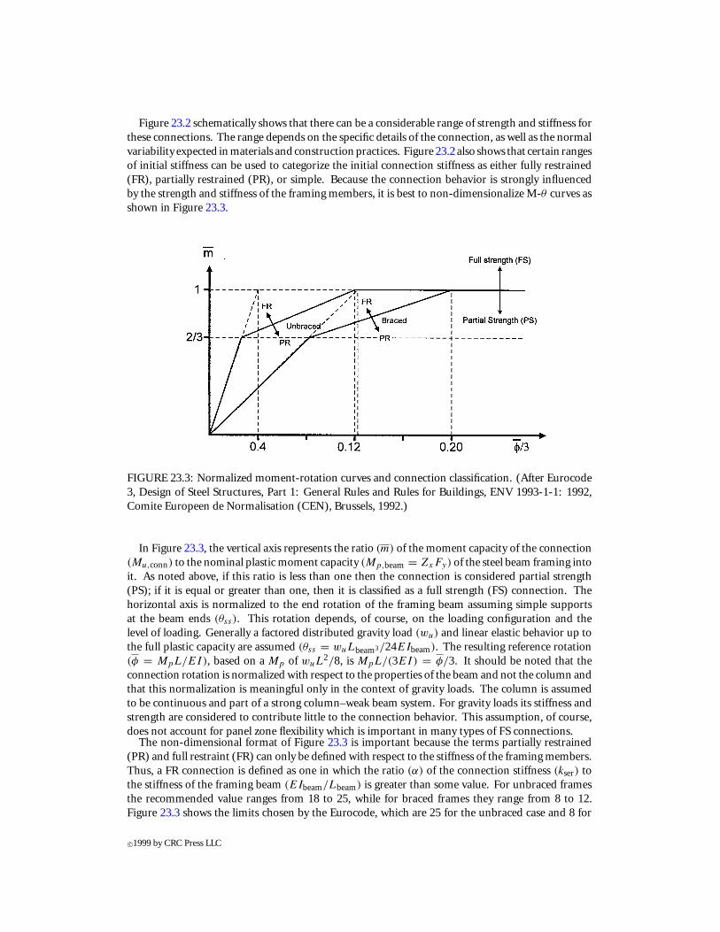
Figure 23.2 schematically shows that there can be a considerable range of strength and stiffness forthese connections. The range depends on the specific details of the connection, as well as the normalvariability expected in materials and construction practices. Figure 23.2 also shows that certain rangesof initial stiffness can be used to categorize the initial connection stiffness as either fully restrained(FR), partially restrained (PR), or simple. Because the connection behavior is strongly influencedby the strength and stiffness of the framing members, it is best to non-dimensionalize M-θ curves asshown in Figure 23.3.

FIGURE 23.3: Normalized moment-rotation curves and connection classification. (After Eurocode3, Design of Steel Structures, Part 1: General Rules and Rules for Buildings, ENV 1993-1-1: 1992,Comite Europeen de Normalisation (CEN), Brussels, 1992.)

In Figure 23.3, the vertical axis represents the ratio (m) of the moment capacity of the connection(Mu,conn) to the nominal plastic moment capacity (Mp,beam = ZxFy) of the steel beam framing intoit. As noted above, if this ratio is less than one then the connection is considered partial strength(PS); if it is equal or greater than one, then it is classified as a full strength (FS) connection. Thehorizontal axis is normalized to the end rotation of the framing beam assuming simple supportsat the beam ends (θss). This rotation depends, of course, on the loading configuration and thelevel of loading. Generally a factored distributed gravity load (wu) and linear elastic behavior up tothe full plastic capacity are assumed (θss = wuLbeam3/24EIbeam). The resulting reference rotation(φ = MpL/EI), based on a Mp of wuL

2/8, is MpL/(3EI) = φ/3. It should be noted that theconnection rotation is normalized with respect to the properties of the beam and not the column andthat this normalization is meaningful only in the context of gravity loads. The column is assumedto be continuous and part of a strong column–weak beam system. For gravity loads its stiffness andstrength are considered to contribute little to the connection behavior. This assumption, of course,does not account for panel zone flexibility which is important in many types of FS connections.

The non-dimensional format of Figure 23.3 is important because the terms partially restrained(PR) and full restraint (FR) can only be defined with respect to the stiffness of the framing members.Thus, a FR connection is defined as one in which the ratio (α) of the connection stiffness (kser) tothe stiffness of the framing beam (EIbeam/Lbeam) is greater than some value. For unbraced framesthe recommended value ranges from 18 to 25, while for braced frames they range from 8 to 12.Figure 23.3 shows the limits chosen by the Eurocode, which are 25 for the unbraced case and 8 for


the braced case [15]. These ranges have been selected based on stability studies that indicate that theglobal buckling load of a frame with PR connections with stiffnesses above these limits is decreasedby less than 5% over the case of a similar frame with rigid connections. The large difference betweenthe braced and unbraced values stems from the P-1 and P-δ effects on the latter. PR connections aredefined as those having α ranging from about 2 up to the FR limit. Connections with α less than 2are regarded as pinned.

23.3 PR Composite Connections

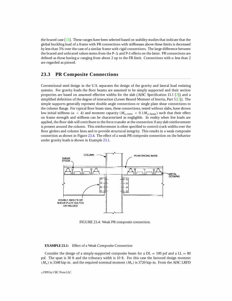
Conventional steel design in the U.S. separates the design of the gravity and lateral load resistingsystems. For gravity loads the floor beams are assumed to be simply supported and their sectionproperties are based on assumed effective widths for the slab (AISC Specification I3.1 [2]) and asimplified definition of the degree of interaction (Lower Bound Moment of Inertia, Part 5 [3]). Thesimple supports generally represent double angle connections or single plate shear connections tothe column flange. For typical floor beam sizes, these connections, tested without slabs, have shownlow initial stiffness (α < 4) and moment capacity (Mu,conn < 0.1Mp,beam) such that their effecton frame strength and stiffness can be characterized as negligible. In reality when live loads areapplied, the floor slab will contribute to the force transfer at the connection if any slab reinforcementis present around the column. This reinforcement is often specified to control crack widths over thefloor girders and column lines and to provide structural integrity. This results in a weak compositeconnection as shown in Figure 23.4. The effect of a weak PR composite connection on the behaviorunder gravity loads is shown in Example 23.1.

FIGURE 23.4: Weak PR composite connection.

EXAMPLE 23.1: Effect of a Weak Composite Connection

Consider the design of a simply-supported composite beam for a DL = 100 psf and a LL = 80psf. The span is 30 ft and the tributary width is 10 ft. For this case the factored design moment(Mu) is 3348 kip-in. and the required nominal moment (Mn) is 3720 kip-in. From the AISC LRFD


Manual [3] one can select an A36 W18x35 composite beam with 92% interaction (PNA = 3, φMp =3720 kip-in., and ILB = 1240 in.4). The W18x35 was selected based on optimizing the section forthe construction loads, including a construction LL allowance of 20 psf. The deflection under the fulllive load for this beam is 0.4 in., well below the 1 in. allowed by the L/360 criterion. Thus, this sectionlooks fine until one starts to check stresses. If we assume that all the dead load stresses from 1.2DL,which are likely to be present after the construction period, are carried by the steel beam alone, then:

σDL,steel alone = MDL/Sx = 1620kip-in. /57.6 in.3 = 28.1 ksi

The stresses from live loads are then superimposed, but on the composite section. For this sectionSeff = 91.9 in.3, so the additional stress due to the arbitrary point-in-time (APT) live load (0.5LL)is:

σLL(APT ) = MLL(APT )/Seff = 540kip-in./91.9 in.3 = 5.9 ksi

Thus, the total stress (σAPT l) under the APT live load is:

σAPT = σDL,steel alone + σLL(APT ) = 28.1 + 5.9 = 34.0 ksi

Under the full live load (1.0LL), the stresses are:

σAPT = σDL,steel alone + 2σLL(APT ) = 28.1 + 11.8 = 39.9 ksi > Fy = 36ksi

Thus, the beam has yielded under the full live loads even though the deflection check seemed to implythat there were no problems at this level. The current LRFD provisions do not include this check,which can govern often if the steel section is optimized for the construction loads.

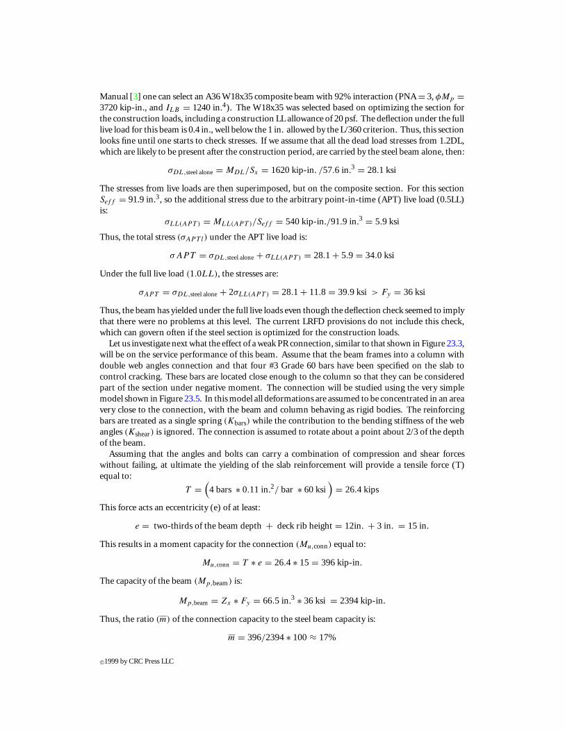
Let us investigate next what the effect of a weak PR connection, similar to that shown in Figure 23.3,will be on the service performance of this beam. Assume that the beam frames into a column withdouble web angles connection and that four #3 Grade 60 bars have been specified on the slab tocontrol cracking. These bars are located close enough to the column so that they can be consideredpart of the section under negative moment. The connection will be studied using the very simplemodel shown in Figure 23.5. In this model all deformations are assumed to be concentrated in an areavery close to the connection, with the beam and column behaving as rigid bodies. The reinforcingbars are treated as a single spring (Kbars) while the contribution to the bending stiffness of the webangles (Kshear) is ignored. The connection is assumed to rotate about a point about 2/3 of the depthof the beam.

Assuming that the angles and bolts can carry a combination of compression and shear forceswithout failing, at ultimate the yielding of the slab reinforcement will provide a tensile force (T)equal to:

T =(4 bars ∗ 0.11 in.2/ bar ∗ 60ksi

)= 26.4 kips

This force acts an eccentricity (e) of at least:

e = two-thirds of the beam depth + deck rib height = 12in. + 3 in. = 15 in.

This results in a moment capacity for the connection (Mu,conn) equal to:

Mu,conn = T ∗ e = 26.4 ∗ 15 = 396kip-in.

The capacity of the beam (Mp,beam) is:

Mp,beam = Zx ∗ Fy = 66.5 in.3 ∗ 36ksi = 2394kip-in.

Thus, the ratio (m) of the connection capacity to the steel beam capacity is:

m = 396/2394∗ 100≈ 17%


FIGURE 23.5: Simple mechanistic connection model.

If we assume that (1) the bars yield and transfer most of their force over a development length of 24bar diameters from the point of inflection, (2) the strain varies linearly, and (3) the connection regionextends for a length equal to the beam depth (18 in.), then the slab reinforcement can be modeledby a spring (Kbars) equal to:

Kbars = EA/L =(30,000ksi ∗ 0.44 in.2

)/(18 in.) = 733.3 kips/in.

Yield will be achieved at a rotation (θy) equal to:

θy = (T / (Kbars ∗ e)) = (26.4 kips/

(733kips/in. × 15 in.

))= 0.0024radians or 2.4 milliradians

The connection stiffness (Kser) can be approximated as:

Kser = Mu,conn/θy = 396kip-in. /0.0024radians = 165,000kip-in./radian

Assuming that the beam spans 30 ft, the beam stiffness is:

Kbeam = EIbeam /Lbeam =(30,000ksi ∗ 510in.4/360in.

)= 42,500kip-in./radian

Thus, the ratio of connection to beam stiffness (α) is:

α = Kser/Kbeam = 165,000/42,500= 3.9

The relatively lowvaluesofα andmobtained for this connection, evenassuming thenon-compositeproperties in order to maximize α and m, would seem to indicate that this connection will have littleeffect on the behavior of the floor system. This is incorrect for two reasons. First, the rotations (0.0024radian) at which the connection strength is achieved are within the service range, and thus muchof the connection strength is activated earlier than for a steel connection. Second, the compositeconnections only work for live loads and thus provide substantial reserve capacity to the system. Themoments at the supports (MPR conn) due to the presence of these weak connections for the case of auniformly distributed load (w) are:

MPR conn = wL2/12∗ 1/ (1 + 2/α) = wL2/18.2


For the case of w being the APT live load, the moment is 238 kip-in., while for the case of the fulllive load it is 476 kip-in. This reduces the moments at the centerline from 540 kip-in. to 302 kip-in.for the APT live load and from 1080 kip-in. to 604 kip-in. for the full live load. The maximumadditional stress is 6.6 ksi under full LL loads, so no yielding will occur. Thus, if a significant portionof the beam’s capacity has been used up by the dead loads, a weak composite connection can preventexcessive deflections at the service level.

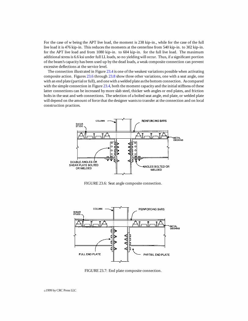
The connection illustrated in Figure 23.4 is one of the weakest variations possible when activatingcomposite action. Figures 23.6 through 23.8 show three other variations, one with a seat angle, onewith an end plate (partial or full), and one with a welded plate as the bottom connection. As comparedwith the simple connection in Figure 23.4, both the moment capacity and the initial stiffness of theselatter connections can be increased by more slab steel, thicker web angles or end plates, and frictionbolts in the seat and web connections. The selection of a bolted seat angle, end plate, or welded platewill depend on the amount of force that the designer wants to transfer at the connection and on localconstruction practices.

FIGURE 23.6: Seat angle composite connection.

FIGURE 23.7: End plate composite connection.


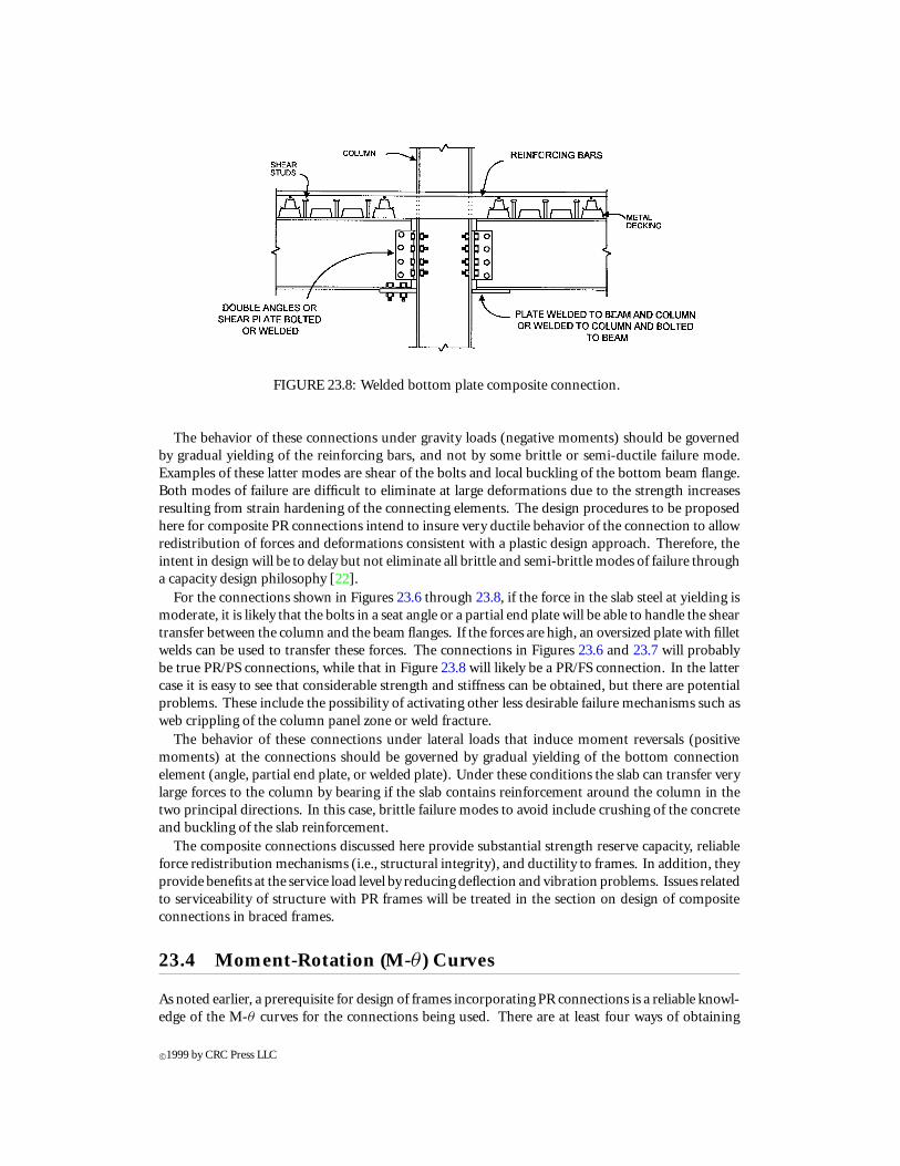
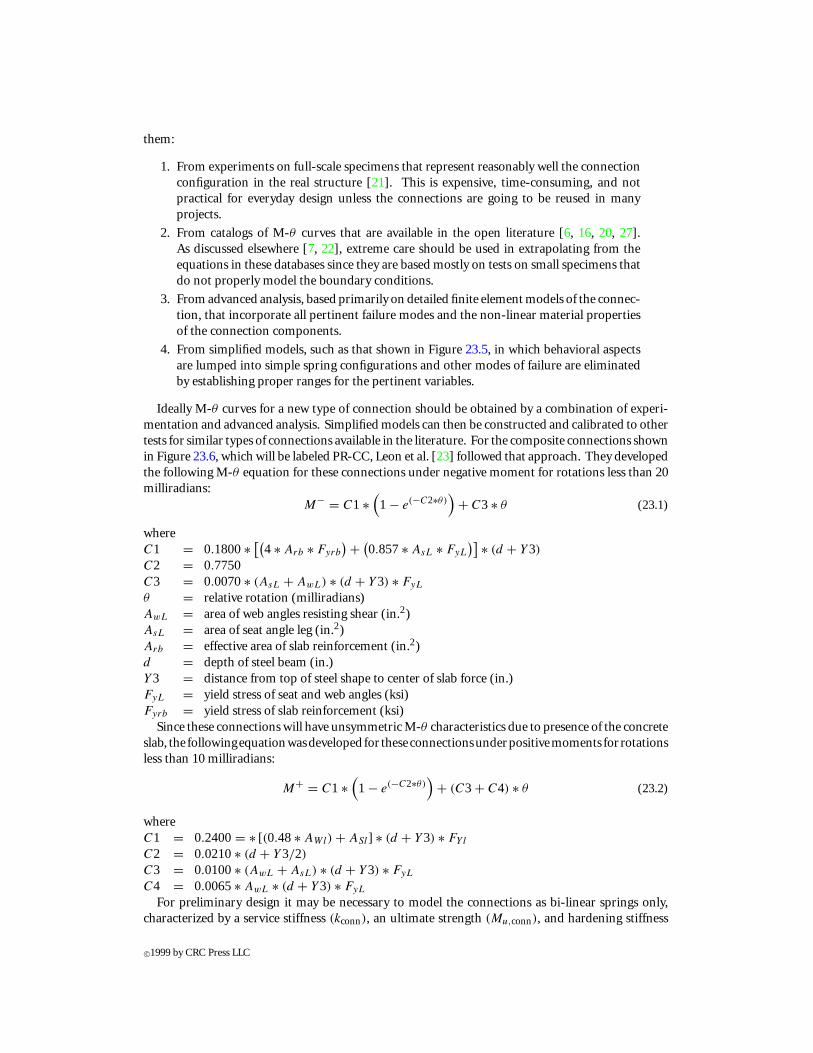
FIGURE 23.8: Welded bottom plate composite connection.

The behavior of these connections under gravity loads (negative moments) should be governedby gradual yielding of the reinforcing bars, and not by some brittle or semi-ductile failure mode.Examples of these latter modes are shear of the bolts and local buckling of the bottom beam flange.Both modes of failure are difficult to eliminate at large deformations due to the strength increasesresulting from strain hardening of the connecting elements. The design procedures to be proposedhere for composite PR connections intend to insure very ductile behavior of the connection to allowredistribution of forces and deformations consistent with a plastic design approach. Therefore, theintent in design will be to delay but not eliminate all brittle and semi-brittle modes of failure througha capacity design philosophy [22].

For the connections shown in Figures 23.6 through 23.8, if the force in the slab steel at yielding ismoderate, it is likely that the bolts in a seat angle or a partial end plate will be able to handle the sheartransfer between the column and the beam flanges. If the forces are high, an oversized plate with filletwelds can be used to transfer these forces. The connections in Figures 23.6 and 23.7 will probablybe true PR/PS connections, while that in Figure 23.8 will likely be a PR/FS connection. In the lattercase it is easy to see that considerable strength and stiffness can be obtained, but there are potentialproblems. These include the possibility of activating other less desirable failure mechanisms such asweb crippling of the column panel zone or weld fracture.

The behavior of these connections under lateral loads that induce moment reversals (positivemoments) at the connections should be governed by gradual yielding of the bottom connectionelement (angle, partial end plate, or welded plate). Under these conditions the slab can transfer verylarge forces to the column by bearing if the slab contains reinforcement around the column in thetwo principal directions. In this case, brittle failure modes to avoid include crushing of the concreteand buckling of the slab reinforcement.

The composite connections discussed here provide substantial strength reserve capacity, reliableforce redistribution mechanisms (i.e., structural integrity), and ductility to frames. In addition, theyprovide benefits at the service load level by reducing deflection and vibration problems. Issues relatedto serviceability of structure with PR frames will be treated in the section on design of compositeconnections in braced frames.

23.4 Moment-Rotation (M-θ ) Curves

As noted earlier, a prerequisite for design of frames incorporating PR connections is a reliable knowl-edge of the M-θ curves for the connections being used. There are at least four ways of obtaining


them:

1. From experiments on full-scale specimens that represent reasonably well the connectionconfiguration in the real structure [21]. This is expensive, time-consuming, and notpractical for everyday design unless the connections are going to be reused in manyprojects.

2. From catalogs of M-θ curves that are available in the open literature [6, 16, 20, 27].As discussed elsewhere [7, 22], extreme care should be used in extrapolating from theequations in these databases since they are based mostly on tests on small specimens thatdo not properly model the boundary conditions.

3. From advanced analysis, based primarily on detailed finite element models of the connec-tion, that incorporate all pertinent failure modes and the non-linear material propertiesof the connection components.

4. From simplified models, such as that shown in Figure 23.5, in which behavioral aspectsare lumped into simple spring configurations and other modes of failure are eliminatedby establishing proper ranges for the pertinent variables.

Ideally M-θ curves for a new type of connection should be obtained by a combination of experi-mentation and advanced analysis. Simplified models can then be constructed and calibrated to othertests for similar types of connections available in the literature. For the composite connections shownin Figure 23.6, which will be labeled PR-CC, Leon et al. [23] followed that approach. They developedthe following M-θ equation for these connections under negative moment for rotations less than 20milliradians:

M− = C1 ∗(1 − e(−C2∗θ)

)+ C3 ∗ θ (23.1)

whereC1 = 0.1800∗ [(4 ∗ Arb ∗ Fyrb

)+ (0.857∗ AsL ∗ FyL

)] ∗ (d + Y3)

C2 = 0.7750C3 = 0.0070∗ (AsL + AwL) ∗ (d + Y3) ∗ FyL

θ = relative rotation (milliradians)AwL = area of web angles resisting shear (in.2)AsL = area of seat angle leg (in.2)Arb = effective area of slab reinforcement (in.2)d = depth of steel beam (in.)Y3 = distance from top of steel shape to center of slab force (in.)FyL = yield stress of seat and web angles (ksi)Fyrb = yield stress of slab reinforcement (ksi)

Since these connections will have unsymmetric M-θ characteristics due to presence of the concreteslab, the followingequationwasdeveloped for theseconnectionsunderpositivemoments for rotationsless than 10 milliradians:

M+ = C1 ∗(1 − e(−C2∗θ)

)+ (C3 + C4) ∗ θ (23.2)

whereC1 = 0.2400= ∗ [(0.48∗ AWl) + ASl ] ∗ (d + Y3) ∗ FYl

C2 = 0.0210∗ (d + Y3/2)

C3 = 0.0100∗ (AwL + AsL) ∗ (d + Y3) ∗ FyL

C4 = 0.0065∗ AwL ∗ (d + Y3) ∗ FyL

For preliminary design it may be necessary to model the connections as bi-linear springs only,characterized by a service stiffness (kconn), an ultimate strength (Mu,conn), and hardening stiffness


(kult). Simplified expressions for these are as follows:

Kconn = 85[(

4ArbFyr

)+ (AwLFyL

)](d + Y3) (23.3)

Mu,conn = 0.245[(

4ArbFyr

)+ (AwLFyL

)](d + Y3) (23.4)

Kult = 12.2[(

4ArbFyr

)+ (AwLFyL

)](d + Y3) (23.5)

For a final check, it is desirable to model the entire response using Equations 23.1 and 23.2 or somepiecewise linear version of them. The author has proposed a tri-linear version for Equation 23.1 forwhich the three breakpoints are defined as [5]:θ1 = the rotation at which the tangent stiffness reaches 80% of its original valueM1 = moment corresponding to θ1θ2 = the rotation at which the exponential term of the connection equations

(e−C2∗q

)is equal

to 0.10M2 = moment corresponding to θ2θ3 = equal to 0.020radians, close to the maximum rotation required for this type of connectionM3 = moment corresponding to θ3

It is necessary in this case to differentiate Equation 23.1 and set θ equal to zero to find an initialstiffness, and then backsolve for the rotation corresponding to 80% of that initial stiffness. All theexamples in this chapter are worked out in English units because metric versions of Equations 23.1through 23.5 have not yet been properly tested.

EXAMPLE 23.2: Moment-Rotation Curves

Figure 23.9b shows the complete M-θ curve for the composite PR connection shown in Fig-ure 23.9a. The values shown in Figure 23.9b were taken directly from substituting into Equations 23.1through 23.4. The shaded squares show the breakpoints for the trilinear curves described in the pre-vious section. The trilinear curve for positive moment was derived by using the same definitionsas for negative moments but limiting the rotations to 10 milliradians, the limit of applicability ofEquation 23.2. Tables for the preliminary and final design of this type of connection are given in arecently issued design guide [26].

The M-θ curves shown in Figure 23.9b are predicated on a certain level of detailing and someassumptions regarding Equations 23.1 through 23.5, including the following:

1. In Equations 23.1 and 23.2, the area of the seat angles (AsL) shall not be taken as morethan 1.5 times that of the reinforcing bars (Arb).

2. In Equations 23.1 and 23.2, the area of the web angles (AwL) resisting shear shall not betaken as more than 1.5 times that of one leg of the seat angle (AsL) for A572 Grade 50steel and 2.0 for Grade A36.

3. The studs shall be designed for full interaction and all provisions of Chapter I of the LRFDSpecification [2] shall be met.

4. All bolts, including those to the beam web, shall be slip-critical and only standard andshort-slotted holes are permitted.

5. Maximum nominal steel yield strength shall be taken as 50 ksi for the beam and 60 ksifor the reinforcing bars. Maximum concrete strength shall be taken as 5 ksi.

6. The slab reinforcement shouldconsistof at least six longitudinalbarsplaced symmetricallywithin a total effective width of seven column flange widths. For edge beams the steelshould be distributed as symmetrically as possible, with at least 1/3 of the total on theedge side.


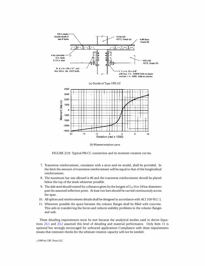
FIGURE 23.9: Typical PR-CC connection and its moment-rotation curves.

7. Transverse reinforcement, consistent with a strut-and-tie model, shall be provided. Inthe limit the amount of transverse reinforcement will be equal to that of the longitudinalreinforcement.

8. The maximum bar size allowed is #6 and the transverse reinforcement should be placedbelow the top of the studs whenever possible.

9. The slab steel should extend for a distance given by the longest ofLb/4 or 24 bar diameterspast the assumed inflection point. At least two bars should be carried continuously acrossthe span.

10. All splices and reinforcement details shall be designed in accordance with ACI 318-95 [1].

11. Whenever possible the space between the column flanges shall be filled with concrete.This aids in transferring the forces and reduces stability problems in the column flangesand web.

These detailing requirements must be met because the analytical studies used to derive Equa-tions 23.1 and 23.2 assumed this level of detailing and material performance. Only Item 11 isoptional but strongly encouraged for unbraced applications Compliance with these requirementsmeans that extensive checks for the ultimate rotation capacity will not be needed.


23.5 Design of Composite Connections in Braced Frames

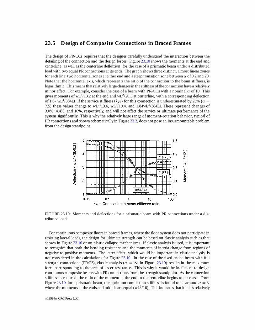
The design of PR-CCs requires that the designer carefully understand the interaction between thedetailing of the connection and the design forces. Figure 23.10 shows the moments at the end andcenterline, as well as the centerline deflection, for the case of a prismatic beam under a distributedload with two equal PR connections at its ends. The graph shows three distinct, almost linear zonesfor each line; two horizontal zones at either end and a steep transition zone between α of 0.2 and 20.Note that the horizontal axis, which represents the ratio of the connection to the beam stiffness, islogarithmic. This means that relatively large changes in the stiffness of the connection have a relativelyminor effect. For example, consider the case of a beam with PR-CCs with a nominal α of 10. Thisgives moments of wL2/13.2 at the end and wL2/20.3 at centerline, with a corresponding deflectionof 1.67 wL4/384EI. If the service stiffness (kser) for this connection is underestimated by 25% (α =7.5) these values change to wL2/13.6, wL2/19.4, and 1.84wL4/384EI. These represent changes of3.0%, 4.4%, and 10%, respectively, and will not affect the service or ultimate performance of thesystem significantly. This is why the relatively large range of moment-rotation behavior, typical ofPR connections and shown schematically in Figure 23.2, does not pose an insurmountable problemfrom the design standpoint.

FIGURE 23.10: Moments and deflections for a prismatic beam with PR connections under a dis-tributed load.

For continuous composite floors in braced frames, where the floor system does not participate inresisting lateral loads, the design for ultimate strength can be based on elastic analysis such as thatshown in Figure 23.10 or on plastic collapse mechanisms. If elastic analysis is used, it is importantto recognize that both the bending resistance and the moments of inertia change from regions ofnegative to positive moments. The latter effect, which would be important in elastic analysis, isnot considered in the calculations for Figure 23.10. In the case of the fixed ended beam with fullstrength connections (FR/FS), elastic analysis (α = ∞ in Figure 23.10) results in the maximumforce corresponding to the area of lesser resistance. This is why it would be inefficient to designcontinuous composite beams with FR connections from the strength standpoint. As the connectionstiffness is reduced, the ratio of the moment at the end to the centerline begins to decrease. FromFigure 23.10, for a prismatic beam, the optimum connection stiffness is found to be around α = 3,where the moments at the ends and middle are equal (wL2/16). This indicates that it takes relatively


little restraint to get a favorable distribution of the loads. If the effect of the changing moments ofinertia is included, as it should for the case of composite beams, the sloping portions of the momentcurves in Figure 23.10 will move to the right. For this case, the optimum solution will not be at theintersection of the M(end) and M (CL) lines but at the location where the ratio of Mp,ci/Mp,b equalsM(end)/ M (CL). Preliminary studies indicate that the optimum connection stiffness for compositebeams is generally found to be still around α of 3 to 6. This indicates that it takes relatively littlerestraint to get a favorable distribution of the loads. This type of simple elastic analysis, however,cannot account for the fact that the connection M-θ curves are non-linear and thus will not be usefulin the analysis of PR/PS connections such as PR-CCs.

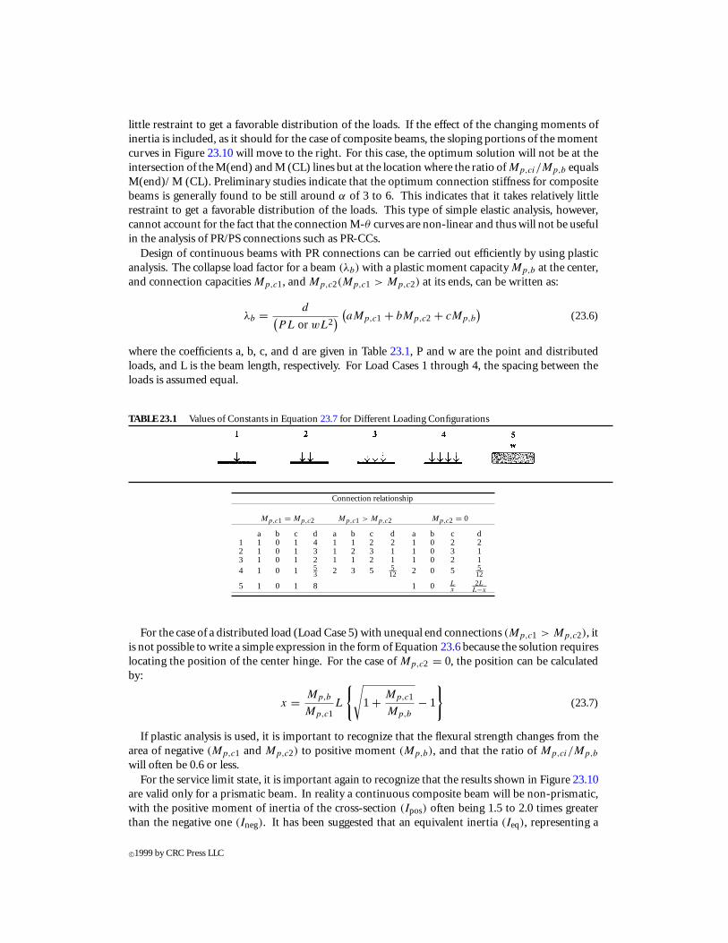
Design of continuous beams with PR connections can be carried out efficiently by using plasticanalysis. The collapse load factor for a beam (λb) with a plastic moment capacity Mp,b at the center,and connection capacities Mp,c1, and Mp,c2(Mp,c1 > Mp,c2) at its ends, can be written as:

λb = d(PL or wL2

) (aMp,c1 + bMp,c2 + cMp,b

)(23.6)

where the coefficients a, b, c, and d are given in Table 23.1, P and w are the point and distributedloads, and L is the beam length, respectively. For Load Cases 1 through 4, the spacing between theloads is assumed equal.

TABLE 23.1 Values of Constants in Equation 23.7 for Different Loading Configurations

Connection relationship

Mp,c1 = Mp,c2 Mp,c1 > Mp,c2 Mp,c2 = 0

a b c d a b c d a b c d1 1 0 1 4 1 1 2 2 1 0 2 22 1 0 1 3 1 2 3 1 1 0 3 13 1 0 1 2 1 1 2 1 1 0 2 14 1 0 1 5

3 2 3 5 512 2 0 5 5

12

5 1 0 1 8 1 0 Lx

2LL−x

For the case of a distributed load (Load Case 5) with unequal end connections (Mp,c1 > Mp,c2), itis not possible to write a simple expression in the form of Equation 23.6 because the solution requireslocating the position of the center hinge. For the case of Mp,c2 = 0, the position can be calculatedby:

x = Mp,b

Mp,c1L

{√1 + Mp,c1

Mp,b

− 1

}(23.7)

If plastic analysis is used, it is important to recognize that the flexural strength changes from thearea of negative (Mp,c1 and Mp,c2) to positive moment (Mp,b), and that the ratio of Mp,ci/Mp,b

will often be 0.6 or less.For the service limit state, it is important again to recognize that the results shown in Figure 23.10

are valid only for a prismatic beam. In reality a continuous composite beam will be non-prismatic,with the positive moment of inertia of the cross-section (Ipos) often being 1.5 to 2.0 times greaterthan the negative one (Ineg). It has been suggested that an equivalent inertia (Ieq), representing a


weighted average, should be used [5]:

Ieq = 0.4Ineg + 0.6Ipos (23.8)

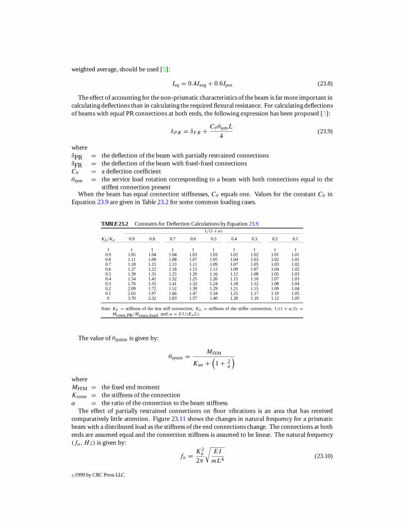
The effect of accounting for the non-prismatic characteristics of the beam is far more important incalculating deflections than in calculating the required flexural resistance. For calculating deflectionsof beams with equal PR connections at both ends, the following expression has been proposed [5]:

δPR = δFR + CθθsymL

4(23.9)

whereδPR = the deflection of the beam with partially restrained connectionsδFR = the deflection of the beam with fixed-fixed connectionsCθ = a deflection coefficientθsym = the service load rotation corresponding to a beam with both connections equal to the

stiffest connection presentWhen the beam has equal connection stiffnesses, Cθ equals one. Values for the constant Cθ in

Equation 23.9 are given in Table 23.2 for some common loading cases.

TABLE 23.2 Constants for Deflection Calculations by Equation 23.91/(1 + α)

Kb/Ka 0.9 0.8 0.7 0.6 0.5 0.4 0.3 0.2 0.1

1 1 1 1 1 1 1 1 1 10.9 1.05 1.04 1.04 1.03 1.03 1.02 1.02 1.01 1.010.8 1.11 1.09 1.08 1.07 1.05 1.04 1.03 1.02 1.010.7 1.18 1.15 1.13 1.11 1.09 1.07 1.05 1.03 1.020.6 1.27 1.22 1.18 1.15 1.12 1.09 1.07 1.04 1.020.5 1.39 1.31 1.25 1.20 1.16 1.12 1.08 1.05 1.030.4 1.54 1.41 1.32 1.25 1.20 1.15 1.10 1.07 1.030.3 1.76 1.55 1.41 1.32 1.24 1.18 1.12 1.08 1.040.2 2.09 1.72 1.52 1.39 1.29 1.21 1.15 1.09 1.040.1 2.63 1.97 1.66 1.47 1.34 1.25 1.17 1.10 1.050 3.70 2.32 1.83 1.57 1.40 1.28 1.19 1.12 1.05

Note: Kb = stiffness of the less stiff connection; Ka = stiffness of the stiffer connection; 1/(1 + α/2) =Mconn,PR/Mconn,fixed and; α = EI/(KaL).

The value of θsymm is given by:

θsymm = MFEM

Kser +(1 + 2

α

)whereMFEM = the fixed end momentKconn = the stiffness of the connectionα = the ratio of the connection to the beam stiffness

The effect of partially restrained connections on floor vibrations is an area that has receivedcomparatively little attention. Figure 23.11 shows the changes in natural frequency for a prismaticbeam with a distributed load as the stiffness of the end connections change. The connections at bothends are assumed equal and the connection stiffness is assumed to be linear. The natural frequency(fn, Hz) is given by:

fn = K2n

2π

√EI

mL4(23.10)


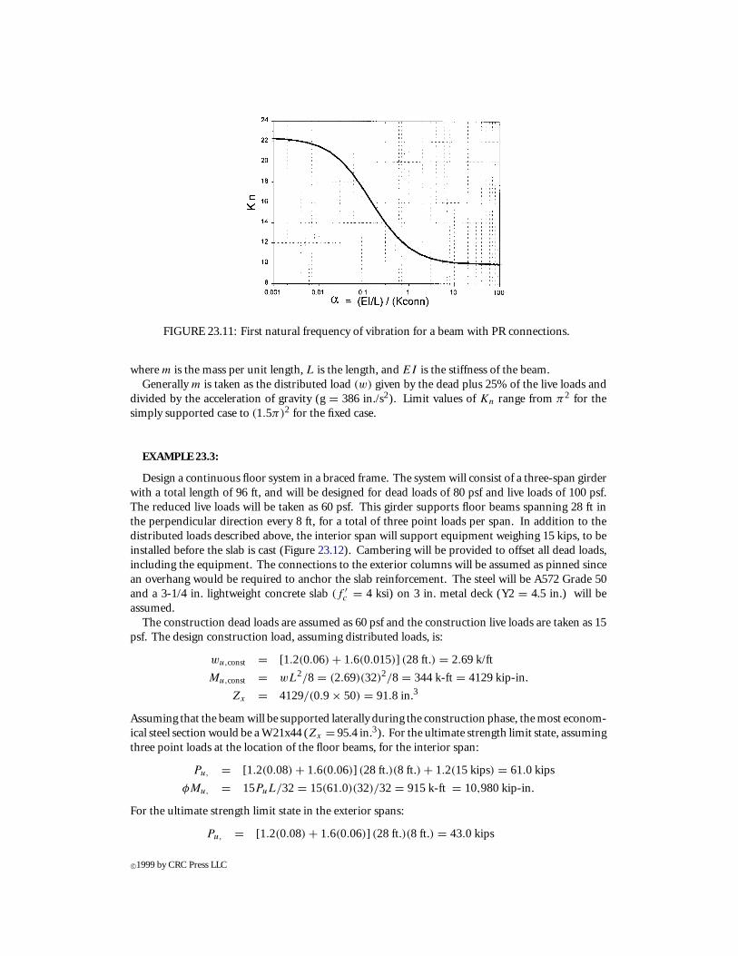
FIGURE 23.11: First natural frequency of vibration for a beam with PR connections.

where m is the mass per unit length, L is the length, and EI is the stiffness of the beam.Generally m is taken as the distributed load (w) given by the dead plus 25% of the live loads and

divided by the acceleration of gravity (g = 386 in./s2). Limit values of Kn range from π2 for thesimply supported case to (1.5π)2 for the fixed case.

EXAMPLE 23.3:

Design a continuous floor system in a braced frame. The system will consist of a three-span girderwith a total length of 96 ft, and will be designed for dead loads of 80 psf and live loads of 100 psf.The reduced live loads will be taken as 60 psf. This girder supports floor beams spanning 28 ft inthe perpendicular direction every 8 ft, for a total of three point loads per span. In addition to thedistributed loads described above, the interior span will support equipment weighing 15 kips, to beinstalled before the slab is cast (Figure 23.12). Cambering will be provided to offset all dead loads,including the equipment. The connections to the exterior columns will be assumed as pinned sincean overhang would be required to anchor the slab reinforcement. The steel will be A572 Grade 50and a 3-1/4 in. lightweight concrete slab (f ′

c = 4 ksi) on 3 in. metal deck (Y2 = 4.5 in.) will beassumed.

The construction dead loads are assumed as 60 psf and the construction live loads are taken as 15psf. The design construction load, assuming distributed loads, is:

wu,const = [1.2(0.06) + 1.6(0.015)] (28 ft.) = 2.69k/ft

Mu,const = wL2/8 = (2.69)(32)2/8 = 344k-ft = 4129kip-in.

Zx = 4129/(0.9 × 50) = 91.8 in.3

Assuming that the beam will be supported laterally during the construction phase, the most econom-ical steel section would be a W21x44 (Zx = 95.4 in.3). For the ultimate strength limit state, assumingthree point loads at the location of the floor beams, for the interior span:

Pu, = [1.2(0.08) + 1.6(0.06)] (28 ft.)(8 ft.) + 1.2(15kips) = 61.0 kips

φMu, = 15PuL/32 = 15(61.0)(32)/32 = 915k-ft = 10,980kip-in.

For the ultimate strength limit state in the exterior spans:

Pu, = [1.2(0.08) + 1.6(0.06)] (28 ft.)(8 ft.) = 43.0 kips


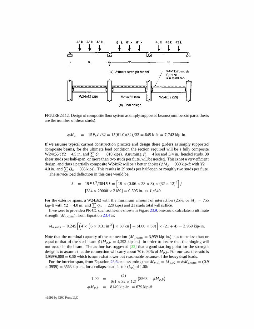
FIGURE 23.12: Design of composite floor system as simply supported beams (numbers in parenthesisare the number of shear studs).

φMu, = 15PuL/32 = 15(61.0)(32)/32 = 645k-ft = 7,742kip-in.

If we assume typical current construction practice and design these girders as simply supportedcomposite beams, for the ultimate load condition the section required will be a fully compositeW24x55 (Y2 = 4.5 in. and

∑Qn = 810 kips). Assuming f ′

c = 4 ksi and 3/4 in. headed studs, 38shear studs per half-span, or more than two studs per flute, will be needed. This is not a very efficientdesign, and thus a partially composite W24x62 will be a better choice (φMp = 930 kip-ft with Y2 =4.0 in. and

∑Qn = 598 kips). This results in 29 studs per half-span or roughly two studs per flute.

The service load deflection in this case would be:

δ = 19PL3/384EI =[19× (0.06× 28× 8) × (32× 12)3

]/

[384× 29000× 2180] = 0.595in. ≈ L/640

For the exterior spans, a W24x62 with the minimum amount of interaction (25%, or Mp = 755kip-ft with Y2 = 4.0 in. and

∑Qn = 228 kips) and 21 studs total will suffice.

If we were to provide a PR-CC such as the one shown in Figure 23.9, one could calculate its ultimatestrength (Mu,conn), from Equation 23.4 as:

Mu,conn = 0.245[(

4 ×(6 × 0.31 in.2

)× 60ksi

)+ (4.00× 50)

]× (21+ 4) = 3,959kip-in.

Note that the nominal capacity of the connection (Mu,conn = 3,959 kip-in.) has to be less than orequal to that of the steel beam φ(Mp,b = 4,293 kip-in.) in order to insure that the hinging willnot occur in the beam. The author has suggested [22] that a good starting point for the strengthdesign is to assume that the connection will carry about 70 to 80% of Mp,b. For our case the ratio is3,959/6,888 = 0.58 which is somewhat lower but reasonable because of the heavy dead loads.

For the interior span, from Equation 23.6 and assuming that Mp,c1 = Mp,c2 = φMu,conn = (0.9× 3959) = 3563 kip-in., for a collapse load factor (λp) of 1.00:

1.00 = (2)

(61× 32× 12)

(3563+ φMp,b

)φMp,b = 8149kip-in. = 679kip-ft


For the exterior span, from Equation 23.6 and assuming that Mp,c1 = 0 and Mp,c2 = φMu,conn =(0.9 × 3959) = 3563 kip-in., for a collapse load factor (λp) of 1.00:

1.00 = (1)

(43× 32× 12)

(3563+ 2φMp,b

)φMp,b = 6474kip-in. = 540kip-ft

The required strength can now be provided by a fully composite W21x44 (φMn = 683 kip-in., and∑Qn = 650 kips or two studs per flute) and by a partially composite W21x44 (φMn = 564 kip-in.,

and∑

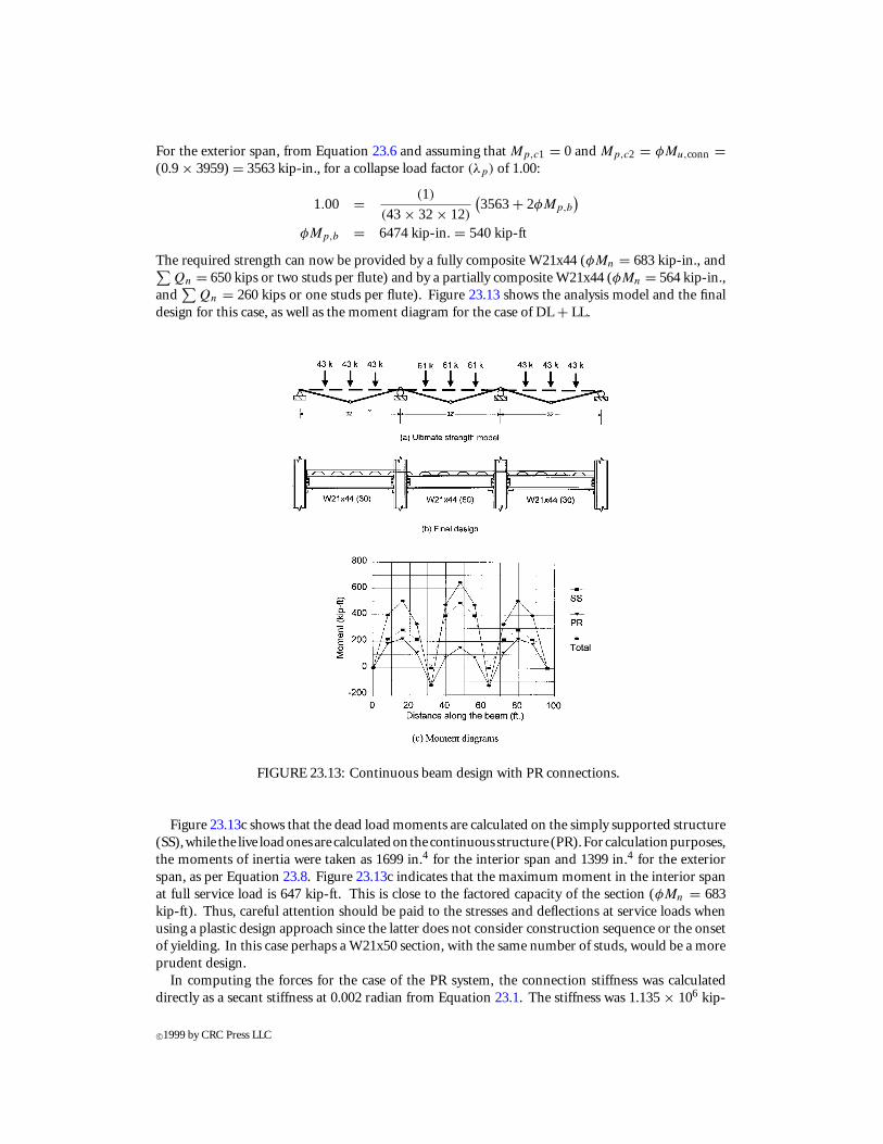
Qn = 260 kips or one studs per flute). Figure 23.13 shows the analysis model and the finaldesign for this case, as well as the moment diagram for the case of DL + LL.

FIGURE 23.13: Continuous beam design with PR connections.

Figure 23.13c shows that the dead load moments are calculated on the simply supported structure(SS),while the live loadonesarecalculatedonthecontinuous structure (PR).Forcalculationpurposes,the moments of inertia were taken as 1699 in.4 for the interior span and 1399 in.4 for the exteriorspan, as per Equation 23.8. Figure 23.13c indicates that the maximum moment in the interior spanat full service load is 647 kip-ft. This is close to the factored capacity of the section (φMn = 683kip-ft). Thus, careful attention should be paid to the stresses and deflections at service loads whenusing a plastic design approach since the latter does not consider construction sequence or the onsetof yielding. In this case perhaps a W21x50 section, with the same number of studs, would be a moreprudent design.

In computing the forces for the case of the PR system, the connection stiffness was calculateddirectly as a secant stiffness at 0.002 radian from Equation 23.1. The stiffness was 1.135 × 106 kip-


in./rad, which is slightly lower than the 1.398 × 106 kip-in./rad given by Equation 23.3. The α forthis connection is:

α = KserL

EI= (1.135× 106)(32× 12)

(29000)(1699)= 8.84

This puts this PR connection near the middle of the PR range for unbraced frames and near the rigidcase for the case of braced frames.

The deflection of the center span under the full live load is, from Equation 23.9:

δPR = PL3

96EI+ CθMFF L

4Kconn

(1 + 2

α

) = 0.161+ 0.109= 0.270in. ≈ L/1500

This deflection is considerably less than that computed for the simply supported case even when amuch larger section (W24x62) was used in the latter case. An idea of the effect of this PR connectioncan be gleaned from inspecting Figure 23.10. Although Figure 23.10 corresponds to a different case,the moment diagrams are not substantially different and thus a meaningful comparison can be madefor the elastic case. From Figure 23.10, the difference in deflection between a simple support and aPR connection with α = 8.84 is roughly a factor of 2.8 (5/1.8), while the difference in moment ofinertia is only 1.28 (2180 in.4 / 1699 in.4). In this example, the design was governed by strength andnot deflections. However, this example clearly shows the impact of a PR connection in reducing floordeflections.

In addition to the strength calculation above, the design procedure requires that the following limitstates and design criteria be satisfied (refer to Figure 23.9a for details):

1. Shear strength of the bolts attaching the seat angle to the beam (φVbolts): The boltshave to be designed to transfer, through shear, a compressive force corresponding to 1.25of the force (Tslab) in the slab reinforcement. The 1.25 factor accounts for the typicaloverstrength of the reinforcement, and intends to insure that the bolts will be able tocarry a force consistent with first yielding of the slab steel. Assuming 1 in. diameterA490N bolts:

(φVbolts) = 1.25Tslab = 1.25FyAbars = 139.5 kips

Nbolts = (φVbolts)/35.3 = 3.95 ∼= 4 bolts (O.K.)

2. Bearing strength at the bolt holes (φRn): The thickness of the angle will be governed bythe required flexural resistance of the angle leg connecting to the beam flange in the case ofa connection in an unbraced frame, where tensile forces at the bottom of the connectionare possible. It will be governed by either bearing of the bolts or compressive yielding ofthe angle leg in the case of a connection in a braced frame. In this case:

φRn = φ(2.4dtFu) = 0.75(2.4 × 0.875× 0.5 × 65)

= 51.2 kips/bolt > φVbolts , O.K.

3. Tension yield and rupture of the seat angle: This limit state is strictly applicable to thecase of unbraced frames where pull-out of the angle under positive moments is possible.For the case of a connection in a braced frame, it is prudent to check the angle for yieldingunder compressive forces (φCn) and possible buckling. The latter is never a problemgiven the short gage lengths, while the former is:

φCn = φ(AgFy

) = 0.9 × (8 × 0.5) × 50 = 180kips > φVbolts , O.K.


4. Number and distribution of slab bars, including transverse reinforcement, to insure aproper strut-and-tie action at ultimate (see section following Example 23.2 for details).

5. Number and distribution of shear studs to provide adequate composite action (checkedabove as part of the flexural design).

6. Tension strength, including prying action, for the bolts connecting the beam to the col-umn.

7. Shear capacity of the web angles.

8. Block shear capacity of the web angles.

9. Check for the need for column stiffeners

Limit states (6) through (9) can be checked following the current LRFD provisions, and the detailswill not be provided here. However, it should be clear from the few calculations shown above thatthe shear capacity of the bolts is the primary mechanism limiting the forces in the connection.

The structural benefitsofusing aPR-CCconnectionare clear fromthe results of this example. Fromthe economic standpoint, for a PR-CC to be beneficial, the cost of the additional reinforcing bars andseat angle bars has to be offset by that of the additional studs and larger sections required for the simplysupported case. In some instances the benefits may not be there from the economic standpoint, butthedesignermaychoose tousePR-CCsanywaybecauseof their additional redundancyand toughness.

In Example 23.3, the design was controlled by strength and thus it was relatively simple to calculateforces based on plastic analysis and proportion the connection based on a simplified model similarto that shown in Figure 23.5. Since deflections did not control the design, the connection stiffnessdid not play an appreciable role in the preliminary design. If serviceability criteria control the design,then the proportioning of the connection can start from Equation 23.3. In this case the analysishas to be iterative, since the value of the connection stiffness will affect the moment diagram andthe deflection. For applications in braced frames, however, experience indicates that it is strengthand not stiffness that governs the design. This is because the steel beam size is controlled by theconstruction loads if the typical unshored construction process is used. In general, the steel beamselected is capable of providing the required stiffness even if it is the minimum amount of interaction(25% is recommended by AISC and 50% by this author).

23.6 Design for Unbraced Frames

As noted earlier, the design of frames with PR connections requires that the effects of the non-linearstiffness andpartial strengthcharacteristicsof the connectionsbe incorporated into theanalysis. Fromthe practical standpoint, the main difference between the design of unbraced FR and PR frames isthe contribution of the connections to the lateral drift. The designer thus needs to balance not justthe stiffness of the columns and beams to satisfy drift requirements, but account for the additionalcontribution of the concentrated rotations at the connections. There are no established practicalrules on the best distribution of resistance to drift between columns, beams, and connections forPR-CCs. Trial designs indicate that distributing them about equally is reasonable (i.e., 33% to thebeams, columns, and connections, respectively), and that it may be advantageous in low-rise framesto count on the columns to carry the majority of the resistance to drift (say 40 to 45% to columns,and the rest divided about equally between the beams and connections). The use of fixed columnbases is imperative in the design of PR-CC frames, just as it is in the design of almost all unbracedFR frames, in order to limit drifts. Thus, designers should pay careful attention to the detailing ofthe foundations and the column bases.

The required level of analysis for the design of unbraced frames with PR connections is currentlynot covered in any detail by design codes. The AISC LRFD specification [2] allows for the use ofsuch connections by requiring that the designer provide a reliable amount of end restraint for the


connectionsbymeansof tests, advancedanalysis, or documented satisfactoryperformance. TheAISCLRFD specification, however, does not provide any guidance on the analysis requirements except tonote that the influence of PR connections on stability and P-1 effects need to be incorporated intothe design. The new NEHRP provisions and AISC seismic provisions [4, 28] will contain genericdesign requirements for frames with PR connections for use in intermediate and ordinary momentframes (IMF and OMF). In addition, it will contain some specific requirements for some specifictypes of connections, such as the PR-CCs described in this chapter. It is unlikely that there will be anattempt in the near future to codify the analysis and design of PR frames since it would be difficult todevelop guidelines to cover the vast array of connection types available (Figure 23.1). Thus, designof PR frames will remain essentially the responsibility of the structural engineer with guidance, forparticular types of connections, from design guidelines [8, 26], books [12, 13, 14], and other technicalpublications. The proposed procedures to be described next remain, therefore, only a suggestionfor proportioning the entire system. Only the detailing of the connections, including checking allpertinent failure modes, should be regarded as a requirement.

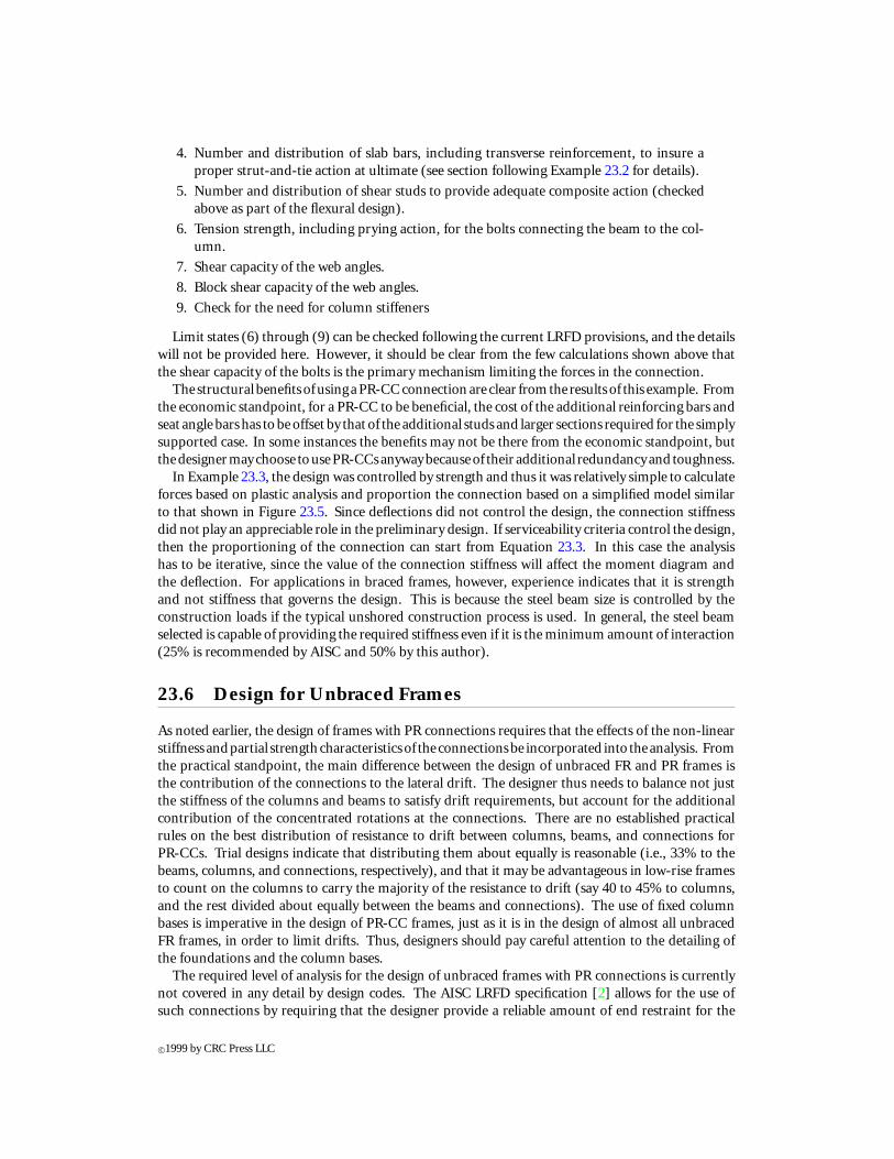
The design procedure to be discussed is divided into two distinct parts. For the service limit states(deflections, drift, and vibrations) the design will use a linear elastic model with elastic rotationalsprings at the beam ends to simulate the influence of the PR connections. For the ultimate limitstates (strength and stability), a modified, second-order plastic analysis approach will be used. Inthis case the connections will be modeled as elastic-perfectly plastic hinges and the stability effectswill be modeled through a simplified second-order approach [26]. Because the latter was calibratedto a population of regular frames with PR-CCs, the approach is only usable for PR-CC frames. Thedesign process will be illustrated with calculations for the frame shown in Figure 23.14. For a completedesign example, including all intermediate steps and design aids, the reader is referred to [26].

EXAMPLE 23.4:

Conduct the preliminary design for the frame shown in Figure 23.14. The frame is a typical interiorframe, has a tributary width of 30 ft, and will be designed for an 80 mph design wind and for forcesconsistent with UBC 1994 seismic zone 2A. The dead loads are 55 psf for the slab and framing and30 psf for partitions, mechanical, and miscellaneous. The weight of the facade is estimated as 700plf. The live loads are 50 psf and 125 psf in the exterior and interior bays, respectively, and will bereduced as per ASCE 7-95. The roof dead and live loads are 30 psf and 20 psf, respectively. The floorslab will consist of a 3-1/4 in. lightweight slab on a 3 in. metal deck, resulting is a typical Y2 for theslab of 4.5 in. The design of the entire frame is beyond the scope of this chapter, so calculations foronly a few key steps will be given.

Part 1: Select beams and determine desired moments at the connections:

Step 1: Select the beam sizes based on the factored construction loads, as illustrated in Exam-ple 23.3. For this case the exterior bays require a W21x50, while the interior bays requirea W21x44.

Step 2: Select moment capacity desired at the supports (Mus) based on the live loads. A goodstarting point is 75% of the Mp of the steel beam selected in Step 1, but the choice is leftto the designer. Once Mus has been chosen, the factored moment at the center of thespan (Muc) can be computed as the difference between the ultimate simply supportedfactored moment (Mu, static moment) and Mus . For the interior span, wu = 6.66 kip/ftand Mu = 1020 kip-ft of which roughly 55% corresponds to the dead loads and 45% tothe live loads. Thus, select a connection capable of carrying:

Mus = 1020× .45× 0.75 = 330kip-ft = 3965kip-in.


FIGURE 23.14: Frame for Example 23.4.

Muc = 1020− 330= 690kip-ft = 8,280kip-in.

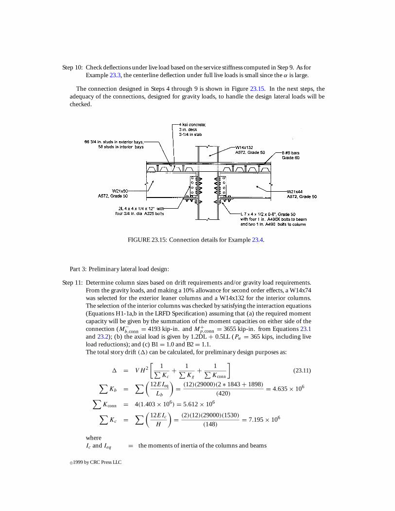
Step 3: Select a composite beam to carry Muc and check that it can carry the unfactored serviceloads without yielding of the slab reinforcement. Assume that full composite actionwill be required to limit vertical deflections and lateral drifts. Using the steel beamsfrom Step 1 and following the procedure from Example 23.3, the exterior bays require aW21x50 with 58 3/4 in. diameter studs, while the interior bays require a W21x44 with52 studs. The design procedure for lateral loads was derived assuming that the beamswere fully composite. In this case that means increasing the number of studs to 66 and58, respectively, which is a very small increase. The moments of inertia computed fromEquation 23.4, and including the contribution of the reinforcement are 1843 in.4 for theW21x44 and 1899 in.4 for the W21x50.

Part 2: Preliminary connection design:

Step 4: Compute the amount of slab reinforcement (Arb) required to carry Mus . Assume thatthe moment arm is equal to the beam depth plus the deck rib height plus 0.5 in. Thenominal required moment capacity is:

Mn = Mus/φ = 3950/0.9 = 4388kip-in.

Arb = 4388/ (60ksi × (21+ 3 + 0.5)) = 2.98 in.2

Try 8 #5 bars (Arb = 2.48 in.2). It is reasonable to use less area than required by theequations above (Arb = 2.98 in.2) because those calculation ignore the contribution ofthe web angles to the ultimate capacity and the φ = 0.9 factor that has been added tothe connection design. The latter accounts for the expected differences in stiffness andstrength for theentire connectionrather than for its individual components. Currently theLRFD Specification does not require such a factor and thus its use, while recommended,is left to the judgment of the designer.

Step 5: Choose a seat angle so that the area of the angle leg (AsL) is capable of transmitting atensile force equal to 1.33 times the force in the slab. The 1.33 factor is used to obtain athicker angle so that its stiffness is increased.

AsL = 2.48∗ (60ksi/50ksi) ∗ 1.33 = 3.95 in.2


Try a L7x4x1/2x8" (AsL = 4.00 in.2).

Step 6: For transferring the shear force consistent with the rebar reaching 1.25Fy , the bolt shearcapacity required is:

Vbolt = 2.48 in.2 × 60ksi × 1.25 = 186kips

This requires four 1-in. A490X bolts. Note that if the number of bolts is taken greaterthan 4, they would be difficult to fit into the commonly available angle shapes. In generalthe number and size of bolts required to carry the shear at the bottom of the connectionis the governing parameter in design. Thus, another possible way of selecting the amountof moment desired at the connection (see Step 2) is to select the size and number of boltsand determine Mus as:

Mus = Vbolt

(beam depth + deck height + 0.5 in.

)Step 7: Determine the number and size of bolts required for the connection to the column flange.

Fromtypical tensioncapacity calculations, includingpryingaction, two1-in. A490Xboltsare required for the connection to the column. In general, and for ease of construction,these bolts should be the same size as those determined from Step 6.

Step 8: Select web angles (AwL) assuming a bearing connection. Check bearing and block shearcapacity. The factored shear (Vu) is:

Vu = 6.6(35/2) = 115.5 kips

The factored shear from lateral loads is based on assuming the formation of a sideswaymechanism in which one end of the beam reaches its positive moment and the otherits negative moment capacity. Since the connection has not been completely designed,assume that thenegative andpositivemoment capacities are the same. This is conservativesince the positive capacity will generally be smaller than the negative one.

Vu = 2Mn,conn/L = (4,388kip-in. + 4,388kip-in.)/(35× 12) = 18.7 kips

From Tables 9-2 in the LRFD Manual, four 3/4 in.-diameter A325N bolts, with a pair ofL4x4x1/4x12" can carry 117 kips. Note that for calculation purposes, the area of the webangles (AWl) in Equations 23.1 and 23.2 is limited to the smallest of the gross shear areaof the angles (2 × 12 × 1/4 = 6.00 in.2) or 1.5 times the area of the seat angle (1.5 ASl =1.5 × 8 × 1/2 = 6.00 in.2). This is required because Equations 23.1 and 23.2 were derivedwith this limit as an assumption.

Step 9: Determine connection strengths and stiffness for preliminary lateral load design. FromEquations 23.3 through 23.5:

kconn = 85[(4 ∗ 2.48∗ 60) + (6 ∗ 50)] (21+ 3.5) = 1.864× 106 kip-in./rad

Mu,conn = 0.245[(4 ∗ 2.48∗ 60) + (6 ∗ 50)] (21+ 3.5) = 5373kip-in.

kult = 12[(4 ∗ 2.48∗ 60) + (6 ∗ 50)] (21+ 3.5) = 263.2 × 103 kip-in./rad

From the more complex Equation 23.1, the ultimate moment at 0.02 radians is 5040kip-in., the secant stiffness to 0.002 radians is 1.403 × 106 kip-in./rad, and the ultimatesecant stiffness is 252 × 103 kip-in./rad. Thus, the approximate formulas seem to providea good preliminary estimate. Whenever possible, the use of Equations 23.1 and 23.2 isrecommended.The stiffness ratio for this connection is:

α = 1.403× 106 × (35× 12)/(29000∗ 1699) = 11.95


Step 10: Check deflections under live load based on the service stiffness computed in Step 9. As forExample 23.3, the centerline deflection under full live loads is small since the α is large.

The connection designed in Steps 4 through 9 is shown in Figure 23.15. In the next steps, theadequacy of the connections, designed for gravity loads, to handle the design lateral loads will bechecked.

FIGURE 23.15: Connection details for Example 23.4.

Part 3: Preliminary lateral load design:

Step 11: Determine column sizes based on drift requirements and/or gravity load requirements.From the gravity loads, and making a 10% allowance for second order effects, a W14x74was selected for the exterior leaner columns and a W14x132 for the interior columns.The selection of the interior columns was checked by satisfying the interaction equations(Equations H1-1a,b in the LRFD Specification) assuming that (a) the required momentcapacity will be given by the summation of the moment capacities on either side of theconnection (M−

b,conn = 4193 kip-in. and M+p,conn = 3655 kip-in. from Equations 23.1

and 23.2); (b) the axial load is given by 1.2DL + 0.5LL (Pu = 365 kips, including liveload reductions); and (c) B1 = 1.0 and B2 = 1.1.The total story drift (1) can be calculated, for preliminary design purposes as:

1 = V H 2[

1∑Kc

+ 1∑Kg

+ 1∑Kconn

](23.11)

∑Kb =

∑(12EIeq

Lb

)= (12)(29000)(2 ∗ 1843+ 1898)

(420)= 4.635× 106

∑Kconn = 4(1.403× 106) = 5.612× 106

∑Kc =

∑(12EIc

H

)= (2)(12)(29000)(1530)

(148)= 7.195× 106

whereIc and Ieq = the moments of inertia of the columns and beams


Lb = the girder lengthH = the story heightV = the story shearkconn = the connection stiffnessFor the girders the effective stiffness of the exterior girders, which are pin-connectedat one end and have a PR connection at the other, was taken as equal to that of onegirder. For the columns, only the two interior ones are used since the exterior ones areleaners. The summations are over all beams, columns, and connections participating inthe lateral load resisting system. Note that for unbraced frames subjected to lateral loadsone connection at each column line will be loading and one will be unloading. Thus,their kconn should be different on either side of a column; however, for preliminary designit is sufficient to assume the kconn for negative moments. For the critical first story, theshear (H) due to the wind loads is 26.3 kips. For drift design, this value will be checkedagainst an allowable drift of 0.25%. From Equation 23.11, the interstory drift is 0.31 in. orH/482which is well within the H/400normally allowed. Note from the calculations ofstiffness in Equation 23.11 that the connections actually provide about 32% of the lateralresistance. The beams provide about 27% and the columns provide the remaining 41%.This represents a well-balanced distribution of stiffness. Note again that the contributionof the columns, which is intimately tied to the assumption of base fixity, is the key tolimiting drifts. The drift under seismic loads (H = 34 kips) can be checked roughly bycalculating the elastic drift and multiplying it by an amplification factor (Cd). The newASIC Seismic and NEHRP provisions give Cd = 5.5 for PR-CCs, and allow a maximumof 1.5% drift for this type of structure. Thus:

1 = (0.31 in. × (34/26.3) × 5.5) = 2.20 in. → (2.20/148) × 100= 1.5%, O.K.

Although this frame barely meets the displacement criteria, a more refined non-linearanalysis should be carried out to determine the actual drift.

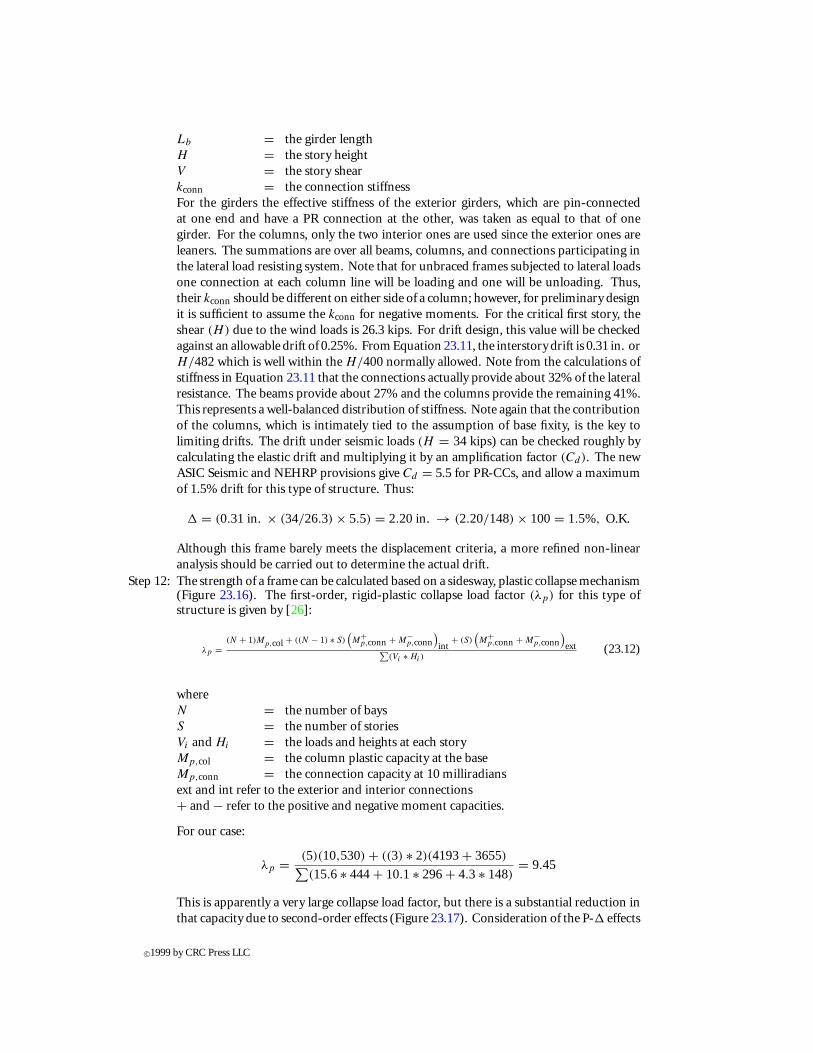
Step 12: The strength of a frame can be calculated based on a sidesway, plastic collapse mechanism(Figure 23.16). The first-order, rigid-plastic collapse load factor (λp) for this type ofstructure is given by [26]:

λp =(N + 1)Mp,col + ((N − 1) ∗ S)

(M+

p,conn + M−p,conn

)int

+ (S)(M+

p,conn + M−p,conn

)ext∑

(Vi ∗ Hi)(23.12)

whereN = the number of baysS = the number of storiesVi and Hi = the loads and heights at each storyMp,col = the column plastic capacity at the baseMp,conn = the connection capacity at 10 milliradiansext and int refer to the exterior and interior connections+ and − refer to the positive and negative moment capacities.

For our case:

λp = (5)(10,530) + ((3) ∗ 2)(4193+ 3655)∑(15.6 ∗ 444+ 10.1 ∗ 296+ 4.3 ∗ 148)

= 9.45

This is apparently a very large collapse load factor, but there is a substantial reduction inthat capacity due to second-order effects (Figure 23.17). Consideration of the P-1 effects


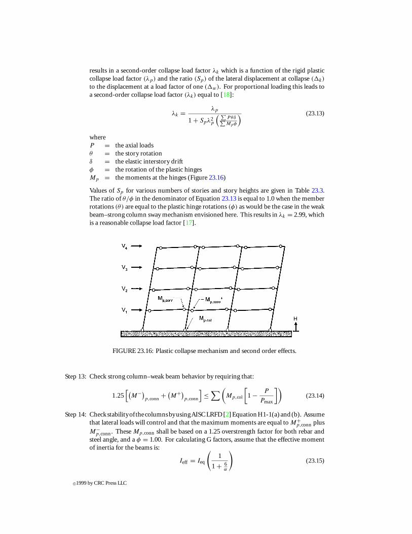
results in a second-order collapse load factor λk which is a function of the rigid plasticcollapse load factor (λp) and the ratio (Sp) of the lateral displacement at collapse (1k)

to the displacement at a load factor of one (1w). For proportional loading this leads toa second-order collapse load factor (λk) equal to [18]:

λk = λp

1 + Spλ2p

( ∑Pθδ∑Mpφ

) (23.13)

whereP = the axial loadsθ = the story rotationδ = the elastic interstory driftφ = the rotation of the plastic hingesMp = the moments at the hinges (Figure 23.16)

Values of Sp for various numbers of stories and story heights are given in Table 23.3.The ratio of θ/φ in the denominator of Equation 23.13 is equal to 1.0 when the memberrotations (θ) are equal to the plastic hinge rotations (φ) as would be the case in the weakbeam–strong column sway mechanism envisioned here. This results in λk = 2.99, whichis a reasonable collapse load factor [17].

FIGURE 23.16: Plastic collapse mechanism and second order effects.

Step 13: Check strong column–weak beam behavior by requiring that:

1.25[(

M−)p,conn

+ (M+)

p,conn

]≤∑(

Mp,col

[1 − P

Pmax

])(23.14)

Step 14: Checkstabilityof thecolumnsbyusingAISCLRFD[2]EquationH1-1(a)and(b). Assumethat lateral loads will control and that the maximum moments are equal to M+

p,conn plus

M−p,conn. These Mp,conn shall be based on a 1.25 overstrength factor for both rebar and

steel angle, and a φ = 1.00. For calculating G factors, assume that the effective momentof inertia for the beams is:

Ieff = Ieq

(1

1 + 6α

)(23.15)


FIGURE 23.17: Simplified computation of plastic second-order effects. (After Horne, M.R. andMorris, L.J. Plastic Design of Low-Rise Frames, The MIT Press, Cambridge, MA, 1982.)

TABLE 23.3 Values of Sp

Number of Story Proportionalstories height (ft) loading

12 84 14 7.2

16 5.412 5.9

6 14 4.516 3.912 3.6

8 14 2.816 2

From Hoffmann, J.J., Design Procedures andAnalysisTools forSemi-RigidCompositeMembers and Frames, M.S. Thesis, Uni-versity of Minnesota, Minneapolis. Withpermission.

Procedures for determining the stability of PR frames are still under development (seeChapter 3 of ASCE 1997 for more details).

Once a preliminary design has been completed, the final checks need to be made with advancedanalysis tools unless the frame is very regular and seismic forces are not a concern. The level ofmodeling required is left to the discretion of the designer, but should, at a minimum, include tri-linear springs to model the connections and include second-order effects.

The design procedures illustrated here are limited to only one type of connection. To the author’sknowledgeonly twoother typesof composite connectionshave receiveda similar levelofdevelopment:those between steel beams and concrete columns and those for composite end plates. An extensivetreatment of the general topic of connection design is given in Chapter 6 of Viest et al. [29]. Thelatest information on design of composite and PR connections can also be found in the proceedingsof several international conferences [9, 10, 11, 19].

References

[1] ACI 318-95. 1995. Building Code Requirements for Reinforced Concrete (ACI 318-95), Amer-ican Concrete Institute, Detroit, MI.


[2] AISC. 1993. Load and Resistance Factor Design Specification for Structural Steel Buildings,2nd. ed., American Institute of Steel Construction, Chicago, IL.

[3] AISC. 1994. Manual of Steel Construction—Load and Resistance Factor Design, 2nd. ed.,American Institute of Steel Construction, Chicago. IL.

[4] AISC. 1997. Seismic Provisions for Structural Steel Building, Load and Resistance FactorDesign, American Institute of Steel Construction, Chicago, IL.

[5] Ammerman, D.J. and Leon, R.T. 1990. Unbraced Frames with Semi-Rigid Connections, AISCEng. J., 27(1), 12-21.

[6] Ang, K. M. and Morris, G. A. 1984. Analysis of Three-Dimensional Frames with Flexible Beam-Column Connections, Can. J. Civ. Eng., 11, 245-254.

[7] ASCE. 1997. Effective Length and Notional Load Approaches for assessing Frame Stability:Implications for American Steel Design, 1st ed., ASCE, New York.

[8] ASCE Task Committee on Design Criteria for Composite Structures in Steel and Concrete.1998, Design Guide for Partially-Restrained Composite Connections (PR-CC), ASCE J. Struc.Eng., to appear in 1998.

[9] Bjorhovde, R., Colson, A., and Zandonini, R., Eds. 1996. Connections in Steel StructuresIII: Behaviour, Strength and Design, Proceedings of the Third International Workshop onConnections held at Trento, Italy, May, 1995, Pergamon Press, London.

[10] Bjorhovde, R., Colson, A., Haaijer, G., and Stark, J.W.B., Eds. 1992. Connections in Steel Struc-tures II: Behaviour, Strength and Design, Proceedings of the Second Workshop on Connectionsheld at Pittsburgh, April 1991, AISC, Chicago, IL.

[11] Bjorhovde, R., Brozzetti, J., and Colson, A., Eds. 1988. Connections in Steel Structures: Be-haviour, Strength and Design, Proceedings of the Workshop on Connections held at the EcoleNormale Superiere, Cachan, France, May 1987, Elsevier Applied Science, London.

[12] Chen, W.F. and Toma, S. 1994. Advanced Analysis of Steel Frames, CRC Press, Boca Raton, FL.[13] Chen, W.F. and Lui, E. 1991. Stability Design of Steel Frames, CRC Press, Boca Raton, FL.[14] Chen, W.F., Goto, Y., and Liew, J. Y. R. 1995. Stability Design of Semi-Rigid Frames, John Wiley

& Sons, New York.[15] Eurocode 3. 1992. Design of Steel Structures, Part 1: General Rules and Rules for Buildings,

ENV 1993-1-1:1992, Comite Europeen de Normalisation (CEN), Brussels.[16] Goverdhan, A.V. 1984. A Collection of Experimental Moment Rotation Curves Evaluation

of Predicting Equations for Semi-Rigid Connections, M.Sc. Thesis, Vanderbilt University,Nashville, TN.

[17] Hoffman, J. J. 1994. Design Procedures and Analysis Tools for Semi-Rigid Composite Membersand Frames, M.S. Thesis, University of Minnesota, Minneapolis.

[18] Horne, M.R. and Morris, L.J. 1982. Plastic Design of Low-Rise Frames, The MIT Press, Cam-bridge, MA.

[19] IABSE. 1989. Bolted and Special Connections, Proceedings of the International Colloquiumheld in Moscow, USSR, May 1989, VNIPIP, 4 Vols., IABSE, Zurich.

[20] Kishi, N. and Chen, W. F. 1986. Data Base of Steel Beam-to-Column Connections, Vol. 1& 2, Structural Engineering Report No. CE-STR-86-26, School of Civil Engineering, PurdueUniversity, West Lafayette, IN.

[21] Leon, R.T. and Deierlein, G.G. 1996. Considerations for the Use of Quasi-Static Testing, Earth-quake Spectra, 12(1), 87-110.

[22] Leon, R.T. 1996. Seismic Performance of Bolted and Riveted Connections, in BackgroundReports onMetallurgy, FractureMechanics, Welding, MomentConnections andFrameSystemBehavior, SAC Report 95-09, SAC Joint Venture, Sacramento, CA.

[23] Leon, R.T., Ammerman, D., Lin, J., andMcCauley, R. 1987. Semi-RigidComposite Steel Frames,AISC Eng. J., 24(4), 147-156.


[24] Leon, R.T. and Hajjar, J.F. 1996. Effect of Floor Slabs on the Performance of Steel MomentConnections, Proceedings of the 11WCEE, Elsevier, London.

[25] Leon, R.T. and Zandonini, R. 1992. Composite Connections, in Steel Design: An InternationalGuide, R. Bjorhovde and P. Dowling, Eds., Elsevier Publishers, London.

[26] Leon, R.T., Hoffman, J., and Staeger, T. 1996. Design of Partially-Restrained Composite Con-nections, AISC Design Guide 9, American Institute of Steel Construction, Chicago, IL.

[27] Nethercot, D.A. 1985. Steel Beam to Column Connections — A Review of Test Data and TheirApplicability to the Evaluation of the Joint Behaviour of the Performance of Steel Frames,CIRIA, London.

[28] HEHRP. 1997. NEHRP Recommended Provisions for Seismic Regulations for New Buildings,BSSC, Washington, D.C.

[29] Viest, I.M., Colaco, J.P., Furlong, R.W., Griffis, L.G., Leon, R.T., and Wyllie, L.A. 1996. Com-posite Construction Design for Buildings, McGraw-Hill, New York.


Leon, R. Composite Connections Structural Engineering ...freeit.free.fr/Structure Engineering...

Documents

Transcript of Leon, R. Composite Connections Structural Engineering ...freeit.free.fr/Structure Engineering...