Lecture 15: Multivariate and Model-based SPC

SpanosEE290H F05

1

Multivariate Control and Model-Based SPC

T2, evolutionary operation, regression chart.

Lecture 15: Multivariate and Model-based SPC

SpanosEE290H F05

2

Multivariate Control

t =(x - µ0)

sx=

(x - µ0)

s2

n

~ t(n-1)

α' = 1 - (1 - α)p

P{all in control} = (1 - α)p

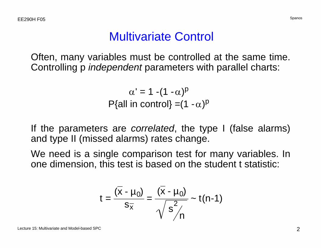
Often, many variables must be controlled at the same time. Controlling p independent parameters with parallel charts:

If the parameters are correlated, the type I (false alarms) and type II (missed alarms) rates change.We need is a single comparison test for many variables. In one dimension, this test is based on the student t statistic:

Lecture 15: Multivariate and Model-based SPC

SpanosEE290H F05

3

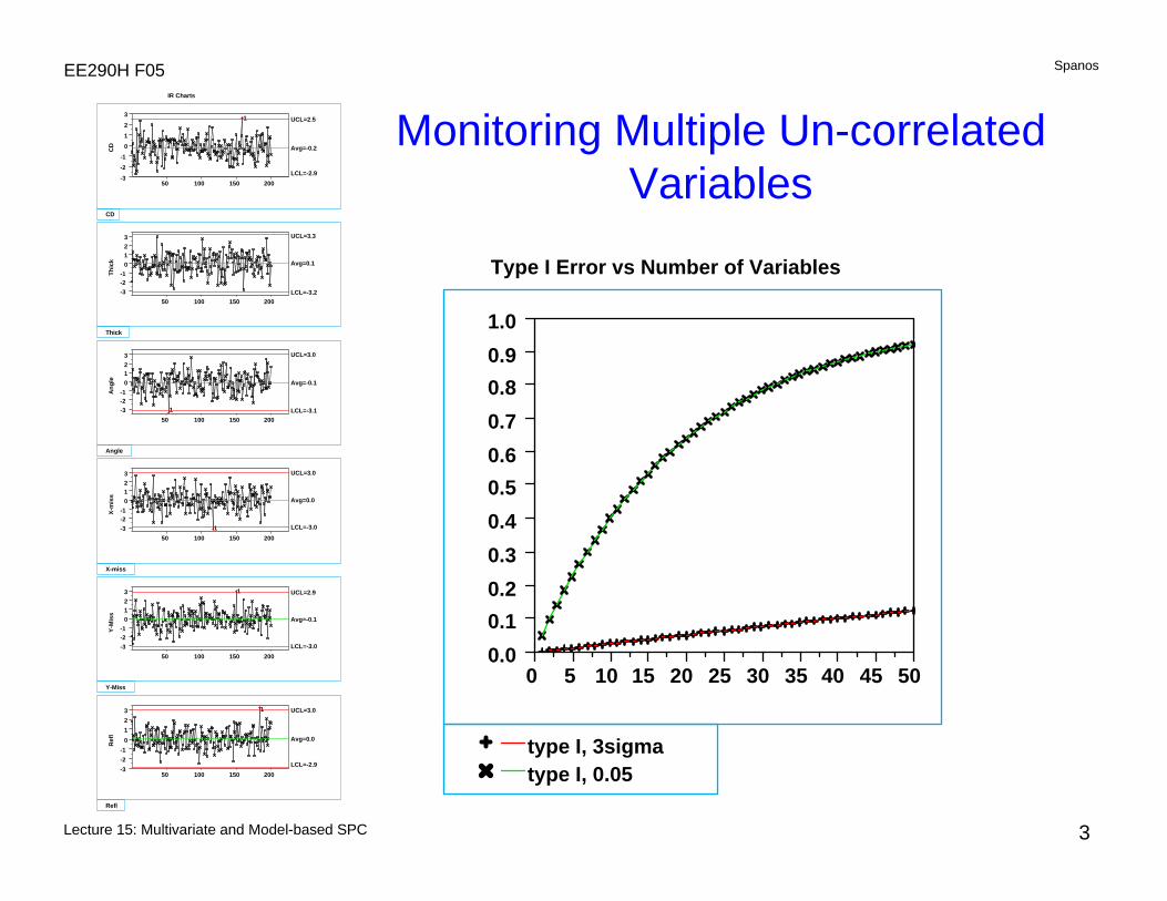
Monitoring Multiple Un-correlated Variables

IR Charts

CD

-3-2-1

0123 1

50 100 150 200

Avg=-0.2

LCL=-2.9

UCL=2.5

CD

Thic

k

-3-2-1

0123

50 100 150 200

Avg=0.1

LCL=-3.2

UCL=3.3

Thick

Ang

le

-3-2-1

0123

150 100 150 200

Avg=-0.1

LCL=-3.1

UCL=3.0

Angle

X-m

iss

-3-2-1

0123

150 100 150 200

Avg=0.0

LCL=-3.0

UCL=3.0

X-miss

Y-M

iss

-3-2-1

0123 1

50 100 150 200

Avg=-0.1

LCL=-3.0

UCL=2.9

Y-Miss

Ref

l

-3-2-1

0123 1

50 100 150 200

Avg=0.0

LCL=-2.9

UCL=3.0

Refl

Type I Error vs Number of Variables

0.00.10.20.30.40.50.60.70.80.91.0

0 5 10 15 20 25 30 35 40 45 50

type I, 3sigmatype I, 0.05

Lecture 15: Multivariate and Model-based SPC

SpanosEE290H F05

4

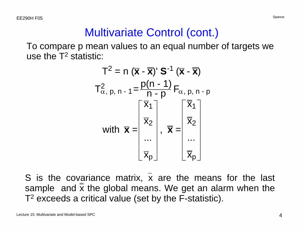
Multivariate Control (cont.)

T2 = n ( x - x)' S-1 (x - x)

Tα, p, n - 12 = p(n - 1)

n - p Fα, p, n - p

with x =

x1

x2

...

xp

, x =

x1

x2

...

xp

S is the covariance matrix, x are the means for the last sample and x the global means. We get an alarm when the T2 exceeds a critical value (set by the F-statistic).

To compare p mean values to an equal number of targets we use the T2 statistic:

Lecture 15: Multivariate and Model-based SPC

SpanosEE290H F05

5

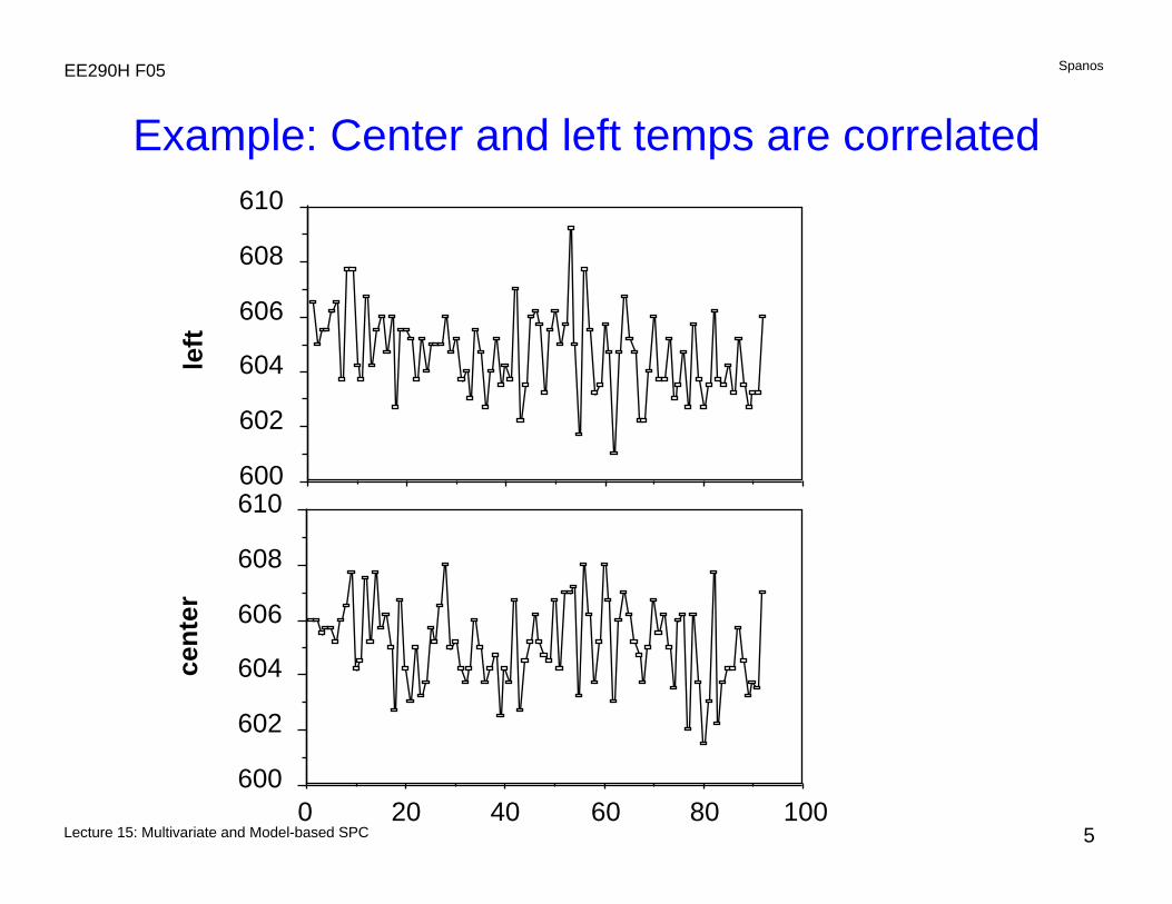
Example: Center and left temps are correlated

600

602

604

606

608

610

100806040200600

602

604

606

608

610

left

cent

er

Lecture 15: Multivariate and Model-based SPC

SpanosEE290H F05

6

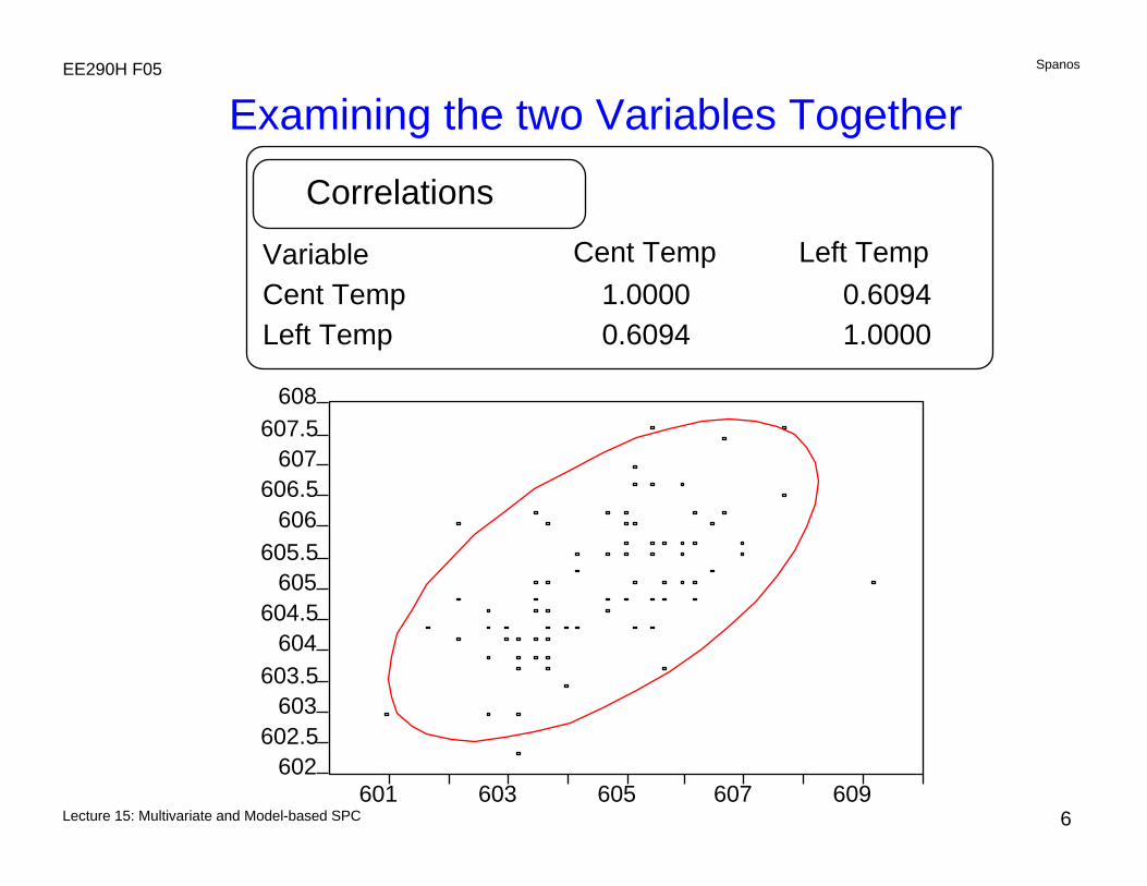
Examining the two Variables Together

Correlations

VariableCent TempLeft Temp

Cent Temp1.00000.6094

Left Temp0.60941.0000

602602.5

603603.5

604604.5

605605.5

606606.5

607607.5

608

601 603 605 607 609

Lecture 15: Multivariate and Model-based SPC

SpanosEE290H F05

7

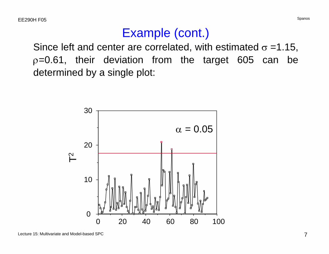
Example (cont.)

α = 0.05

Since left and center are correlated, with estimated σ =1.15, ρ=0.61, their deviation from the target 605 can be determined by a single plot:

1008060402000

10

20

30

T2

Lecture 15: Multivariate and Model-based SPC

SpanosEE290H F05

8

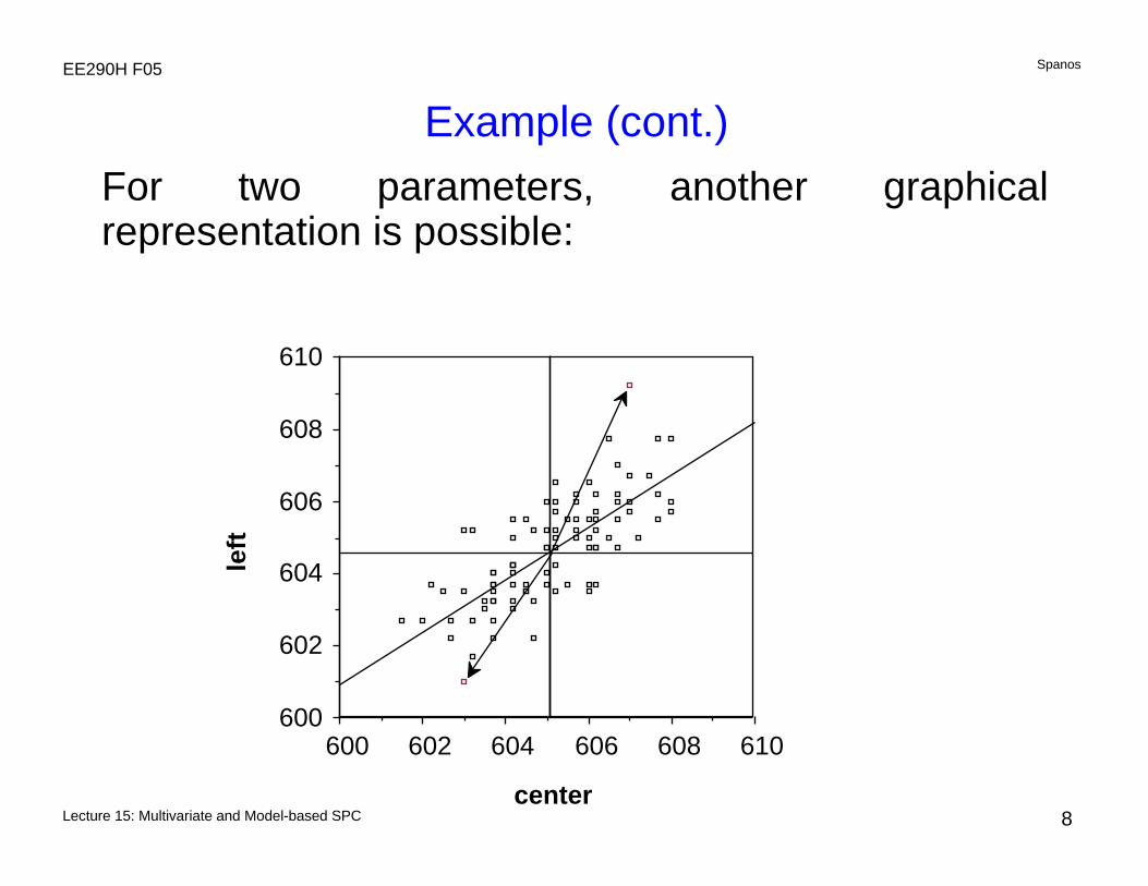
Example (cont.)For two parameters, another graphical representation is possible:

610608606604602600600

602

604

606

608

610

center

left

Lecture 15: Multivariate and Model-based SPC

SpanosEE290H F05

9

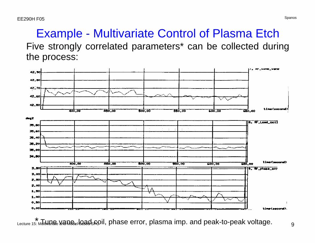
Example - Multivariate Control of Plasma Etch

Haifang's Screen Dump

Five strongly correlated parameters* can be collected during the process:

* Tune vane, load coil, phase error, plasma imp. and peak-to-peak voltage.

Lecture 15: Multivariate and Model-based SPC

SpanosEE290H F05

10

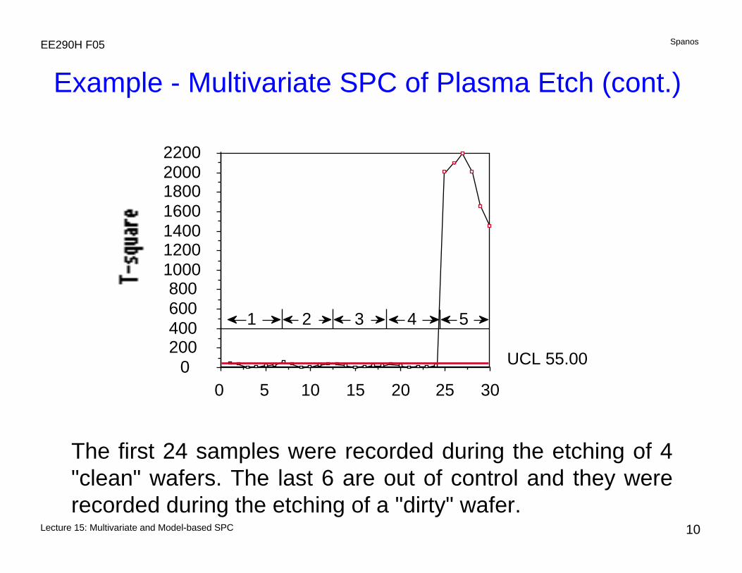
Example - Multivariate SPC of Plasma Etch (cont.)

The first 24 samples were recorded during the etching of 4 "clean" wafers. The last 6 are out of control and they were recorded during the etching of a "dirty" wafer.

3025201510500

200400600800

1000120014001600180020002200

UCL 55.00

1 2 3 4 5

Lecture 15: Multivariate and Model-based SPC

SpanosEE290H F05

11

Evolutionary Operation - An SPC/DOE Application

y = f (x1, x2) + e

and assume the following approximate model:

y - a x1 + b x2 + c x1x2

If we knew a, b, and c, we would know how to change the process in order to bring y closer to the specifications.Of course this model will only be applicable for a narrowrange of the input parameters.

A process can be optimized on-line, by inducing small changes and accepting the ones that improve its quality.EVOP can be seen as an on-line application of designed experiments.Example: Assume a two-parameter process:

Lecture 15: Multivariate and Model-based SPC

SpanosEE290H F05

12

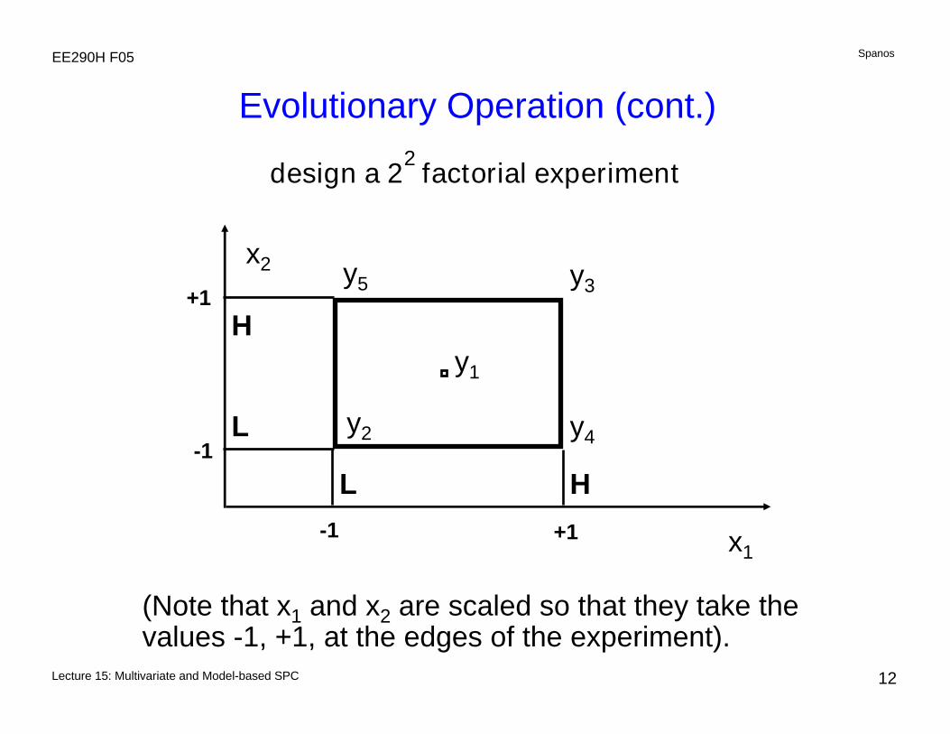
Evolutionary Operation (cont.)

design a 22 factorial experiment

x2

x1

y5 y3

y2 y4

y1

L H

L

H

+1-1

+1

-1

(Note that x1 and x2 are scaled so that they take the values -1, +1, at the edges of the experiment).

Lecture 15: Multivariate and Model-based SPC

SpanosEE290H F05

13

Evolutionary Operation (cont.)

x2

x1

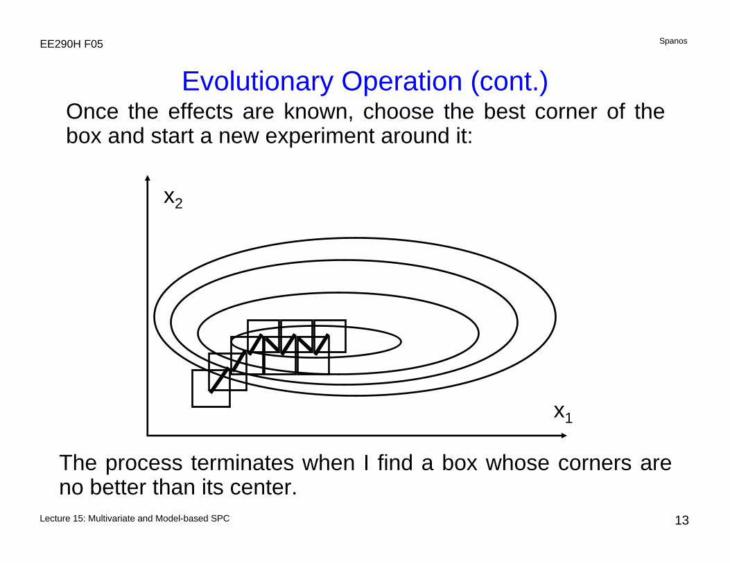
The process terminates when I find a box whose corners are no better than its center.

Once the effects are known, choose the best corner of the box and start a new experiment around it:

Lecture 15: Multivariate and Model-based SPC

SpanosEE290H F05

14

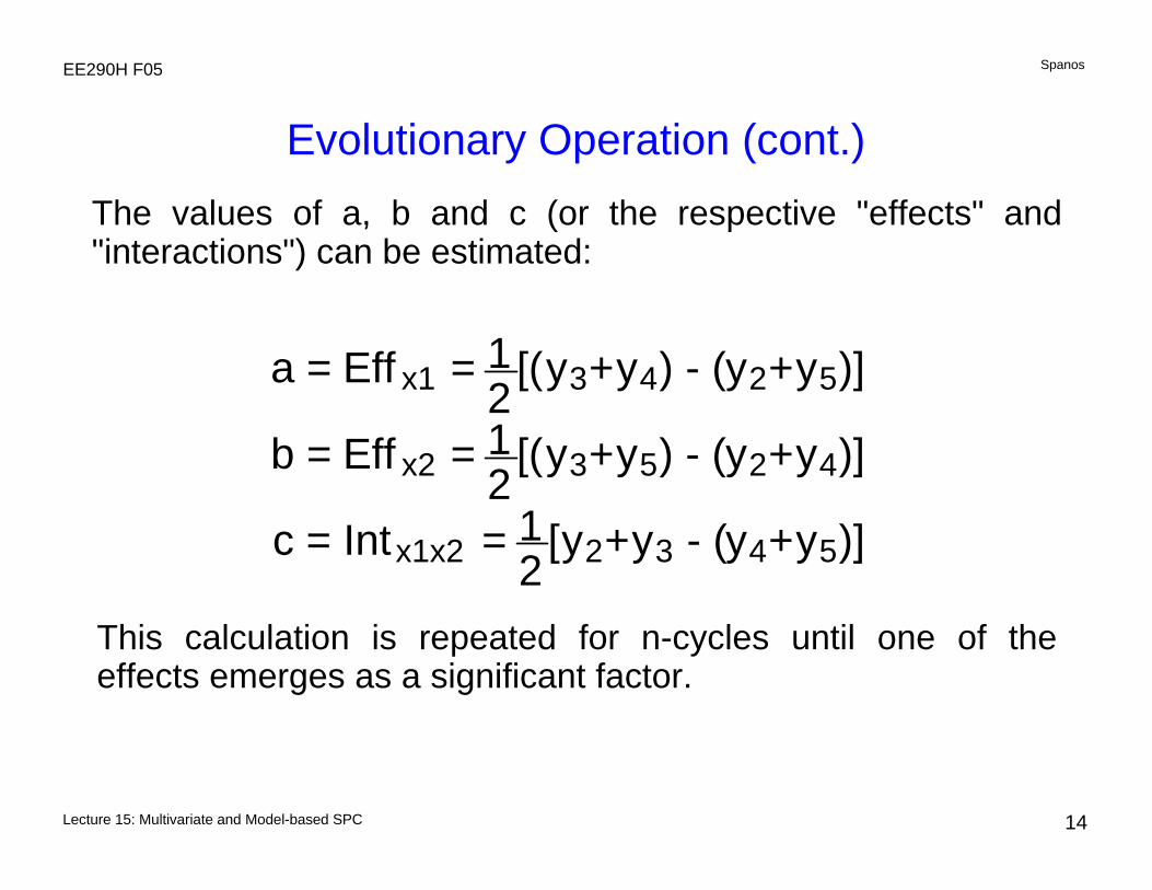
Evolutionary Operation (cont.)The values of a, b and c (or the respective "effects" and "interactions") can be estimated:

This calculation is repeated for n-cycles until one of the effects emerges as a significant factor.

a = Eff x1 = 12

[(y3+y4) - (y2+y5)]

b = Eff x2 = 12

[(y3+y5) - (y2+y4)]

c = Intx1x2 = 12

[y2+y3 - (y4+y5)]

Lecture 15: Multivariate and Model-based SPC

SpanosEE290H F05

15

Evolutionary Operation (cont.)

+/-

+/-

N ( 0, σ2 nn - 1

)

2ns

1.78n s

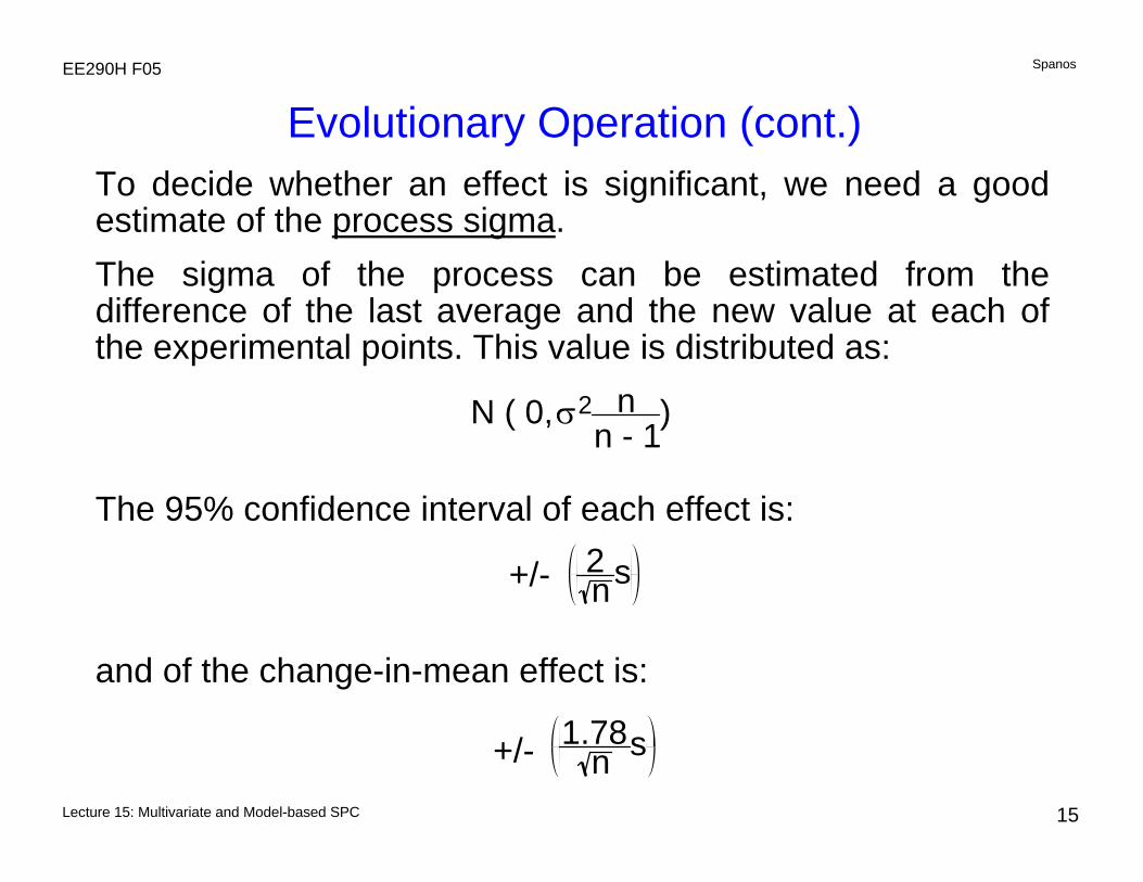
To decide whether an effect is significant, we need a good estimate of the process sigma.The sigma of the process can be estimated from the difference of the last average and the new value at each of the experimental points. This value is distributed as:

The 95% confidence interval of each effect is:

and of the change-in-mean effect is:

Lecture 15: Multivariate and Model-based SPC

SpanosEE290H F05

16

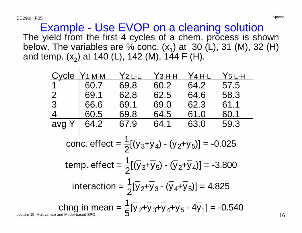
Example - Use EVOP on a cleaning solution

conc. effect = 12[(y3+y4) - (y2+y5)] = -0.025

temp. effect = 12[(y3+y5) - (y2+y4)] = -3.800

interaction = 12[y2+y3 - (y4+y5)] = 4.825

chng in mean = 15[y2+y3+y4+y5 - 4y1] = -0.540

The yield from the first 4 cycles of a chem. process is shown below. The variables are % conc. (x1) at 30 (L), 31 (M), 32 (H) and temp. (x2) at 140 (L), 142 (M), 144 F (H).

Cycle Y1 M-M Y2 L-L Y3 H-H Y4 H-L Y5 L-H1 60.7 69.8 60.2 64.2 57.52 69.1 62.8 62.5 64.6 58.33 66.6 69.1 69.0 62.3 61.14 60.5 69.8 64.5 61.0 60.1avg Y 64.2 67.9 64.1 63.0 59.3

Lecture 15: Multivariate and Model-based SPC

SpanosEE290H F05

17

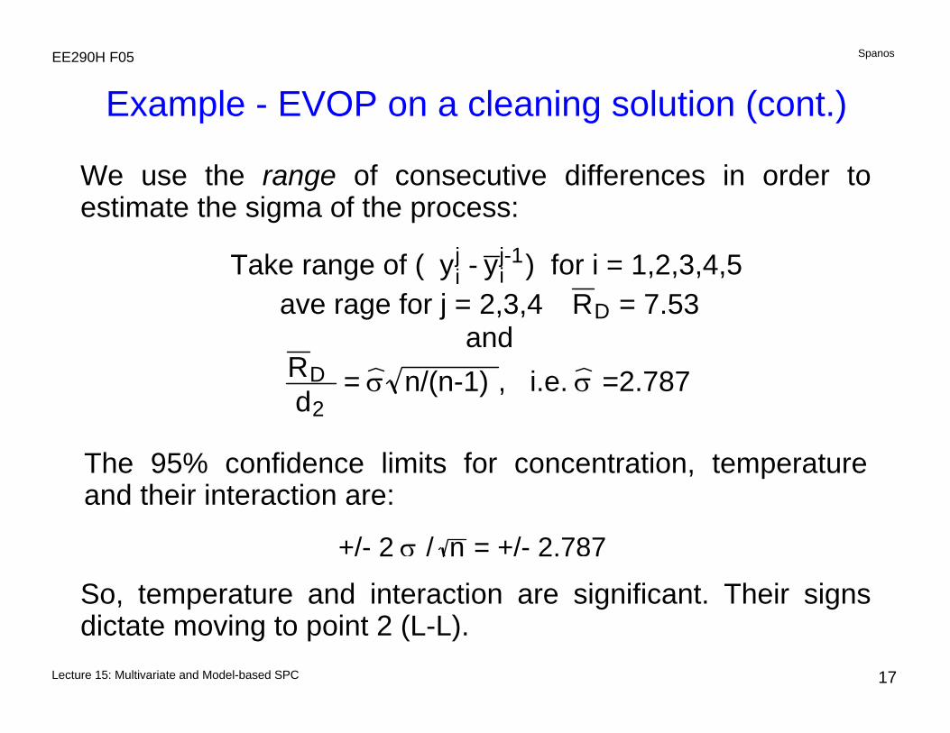
Example - EVOP on a cleaning solution (cont.)

+/- 2 σ / n = +/- 2.787

Take range of ( yij - yi

j-1) for i = 1,2,3,4,5ave rage for j = 2,3,4 RD = 7.53

andRD d2

= σ n/(n-1) , i.e. σ =2.787

So, temperature and interaction are significant. Their signs dictate moving to point 2 (L-L).

The 95% confidence limits for concentration, temperature and their interaction are:

We use the range of consecutive differences in order to estimate the sigma of the process:

Lecture 15: Multivariate and Model-based SPC

SpanosEE290H F05

18

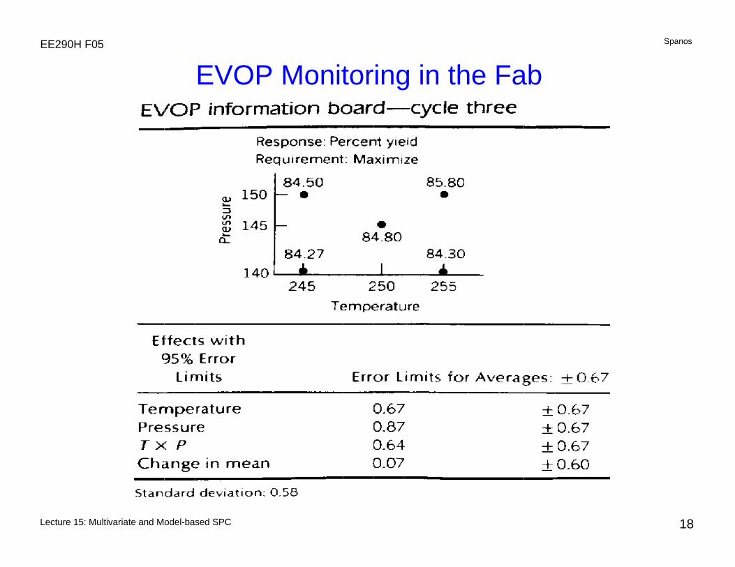
EVOP Monitoring in the Fab

Lecture 15: Multivariate and Model-based SPC

SpanosEE290H F05

19

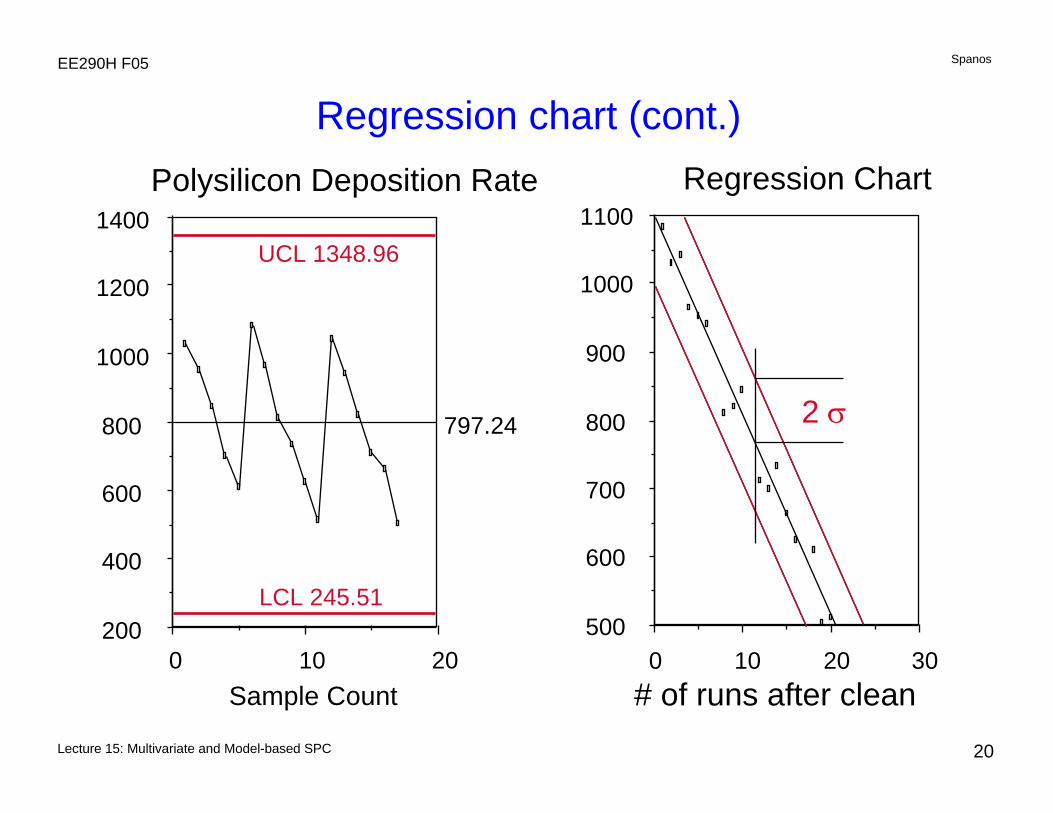
Regression Chart - Model Based SPC

In typical SPC, we try to establish that certain process responses stay on target.What happens if there is one assignable cause that we know and we can quantify? If, for example, the deposition rate of poly is a function of the time since the last tube cleaning, it will never be "in control".In cases like this, we build a regression model of the response vs the known effect, and we try to establish that the regression model remains valid throughout the operation. Limits around the regression line are set according to the prediction error of the model.A t-statistic is used to update the model whenever necessary.

Lecture 15: Multivariate and Model-based SPC

SpanosEE290H F05

20

Regression chart (cont.)

20100200

400

600

800

1000

1200

1400Polysilicon Deposition Rate

Sample Count

LCL 245.51

797.24

UCL 1348.96

3020100500

600

700

800

900

1000

1100Regression Chart

# of runs after clean

2 σ

Lecture 15: Multivariate and Model-based SPC

SpanosEE290H F05

21

Regression Chart (cont.)

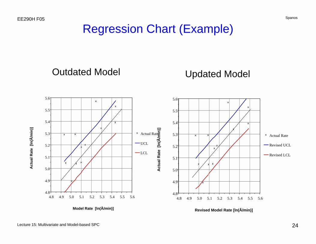
• The regression chart can be generalized for complex equipment models.

• An empirical model is built to describe the changing aspects of the process.

• The difference between prediction and observation can be used as the control statistic

• If the control statistic becomes consistently different than zero, its value can be used to update the model.

Lecture 15: Multivariate and Model-based SPC

SpanosEE290H F05

22

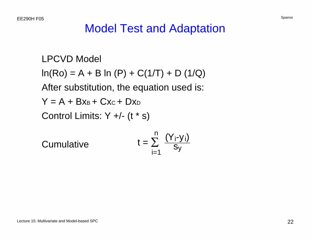
Model Test and Adaptation

LPCVD Modelln(Ro) = A + B ln (P) + C(1/T) + D (1/Q)After substitution, the equation used is:Y = A + BxB + CxC + DxD

Control Limits: Y +/- (t * s)

Cumulative t = (Yi-yi)syΣ

i=1

n

Lecture 15: Multivariate and Model-based SPC

SpanosEE290H F05

23

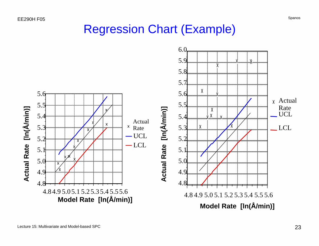
Regression Chart (Example)

5.65.55.45.35.25.15.04.94.8

4.84.95.05.15.25.35.4

5.55.65.75.85.96.0

Actual RateUCL

LCL

Model Rate [ln(Å/min)]

Act

ual R

ate

[ln(

Å/m

in)]

5.65.55.45.35.25.15.04.94.84.8

4.95.0

5.15.2

5.3

5.45.5

5.6

Actual RateUCLLCL

Model Rate [ln(Å/min)]

Act

ual R

ate

[ln(

Å/m

in)]

Lecture 15: Multivariate and Model-based SPC

SpanosEE290H F05

24

Regression Chart (Example)

5.65.55.45.35.25.15.04.94.84.8

4.9

5.0

5.1

5.2

5.3

5.4

5.5

5.6

Actual Rate

UCL

LCL

Model Rate [ln(Å/min)]

Act

ual R

ate

[ln(

Å/m

in)]

5.65.55.45.35.25.15.04.94.84.8

4.9

5.0

5.1

5.2

5.3

5.4

5.5

5.6

Actual Rate

Revised UCL

Revised LCL

Revised Model Rate [ln(Å/min)]

Act

ual R

ate

[ln(

Å/m

in)]

Outdated Model Updated Model

Lecture 15: Multivariate and Model-based SPC

SpanosEE290H F05

25

Summary so far...

As we move from classical, human operator orientedtechniques, to more automated CIM based approaches:

• We need to increase sensitivity (reduce type II error), without increasing type I error. (CUSUM, EWMA).

• We need to distinguish between abrupt and gradual changes. (Choice of EWMA shape).

• We need to accommodate multiple sensor readings (T2

chart).

• We need to accommodate multiple recipes and products in each process (EVOP, model-based SPC).