LEAST-SQUARES FINITE ELEMENT METHODS FOR THE

POISSON EQUATION AND THEIR CONNECTION TO

THE DIRICHLET AND KELVIN PRINCIPLES

Max Gunzburger

School of Computational Science

Florida State University

Joint work with

Pavel BochevComputational Mathematics and Algorithms Department

Sandia National Laboratories

Last updated in 2007

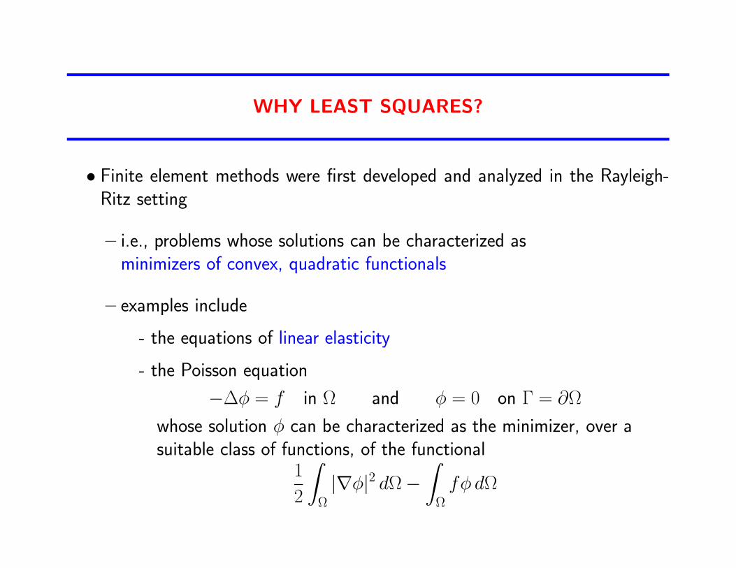
WHY LEAST SQUARES?

• Finite element methods were first developed and analyzed in the Rayleigh-Ritz setting

– i.e., problems whose solutions can be characterized asminimizers of convex, quadratic functionals

– examples include

- the equations of linear elasticity

- the Poisson equation

−∆φ = f in Ω and φ = 0 on Γ = ∂Ω

whose solution φ can be characterized as the minimizer, over asuitable class of functions, of the functional

1

2

∫

Ω

|∇φ|2 dΩ−

∫

Ω

fφ dΩ

• The Rayleigh-Ritz setting results in finite element methods having the fol-lowing desirable features

1. general regions and boundary conditions are relatively easy to handle andhigher-order accuracy is relatively easy to achieve

2. the conformity of the finite element spaces are sufficient to guaranteestability and optimal accuracy

3. all variables can be approximated using a single type of finite elementspace, i.e., based on the same grid and same degree polynomials

4. the resulting linear systems are

a) sparse; b) symmetric; c) positive definite

• FEMs were quickly applied in other settings,

– motivated by the fact that properties 1 and 4a are retained for all FEMs

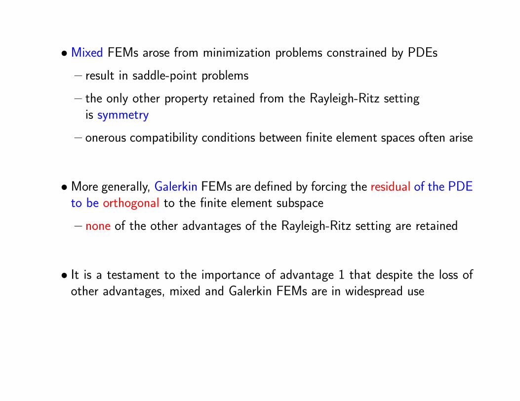
•Mixed FEMs arose from minimization problems constrained by PDEs

– result in saddle-point problems

– the only other property retained from the Rayleigh-Ritz settingis symmetry

– onerous compatibility conditions between finite element spaces often arise

•More generally, Galerkin FEMs are defined by forcing the residual of the PDEto be orthogonal to the finite element subspace

– none of the other advantages of the Rayleigh-Ritz setting are retained

• It is a testament to the importance of advantage 1 that despite the loss ofother advantages, mixed and Galerkin FEMs are in widespread use

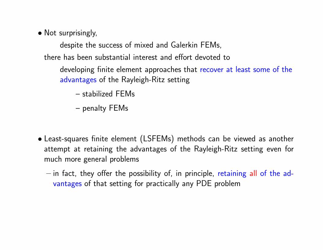
• Not surprisingly,

despite the success of mixed and Galerkin FEMs,

there has been substantial interest and effort devoted to

developing finite element approaches that recover at least some of theadvantages of the Rayleigh-Ritz setting

– stabilized FEMs

– penalty FEMs

• Least-squares finite element (LSFEMs) methods can be viewed as anotherattempt at retaining the advantages of the Rayleigh-Ritz setting even formuch more general problems

– in fact, they offer the possibility of, in principle, retaining all of the ad-vantages of that setting for practically any PDE problem

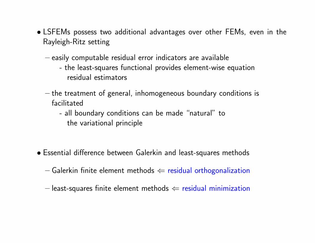
• LSFEMs possess two additional advantages over other FEMs, even in theRayleigh-Ritz setting

– easily computable residual error indicators are available- the least-squares functional provides element-wise equation

residual estimators

– the treatment of general, inhomogeneous boundary conditions isfacilitated

- all boundary conditions can be made “natural” tothe variational principle

• Essential difference between Galerkin and least-squares methods

– Galerkin finite element methods ⇐ residual orthogonalization

– least-squares finite element methods ⇐ residual minimization

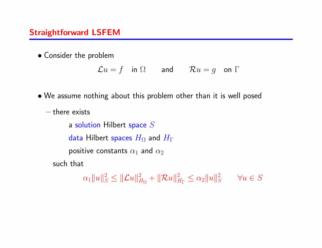
Straightforward LSFEM

• Consider the problem

Lu = f in Ω and Ru = g on Γ

•We assume nothing about this problem other than it is well posed

– there exists

a solution Hilbert space S

data Hilbert spaces HΩ and HΓ

positive constants α1 and α2

such that

α1‖u‖2S ≤ ‖Lu‖

2HΩ

+ ‖Ru‖2HΓ≤ α2‖u‖

2S ∀u ∈ S

• Now, consider the least-squares functional

J(u; f, g) = ‖Lu− f‖2HΩ+ ‖Ru− g‖2HΓ

and the unconstrained minimization problem

minu∈S

J(u; f, g)

so that

(Lv,Lu)HΩ+ (Rv,Ru)HΓ

= (Lv, f)HΩ+ (Rv, g)HΓ

∀ v ∈ S

– note that

the spaces used to measure the sizes of the residuals arethe data spaces HΩ and HΓ

and

the space in which candidate minimizers are sought isthe solution space S

for which the PDE problem is well posed

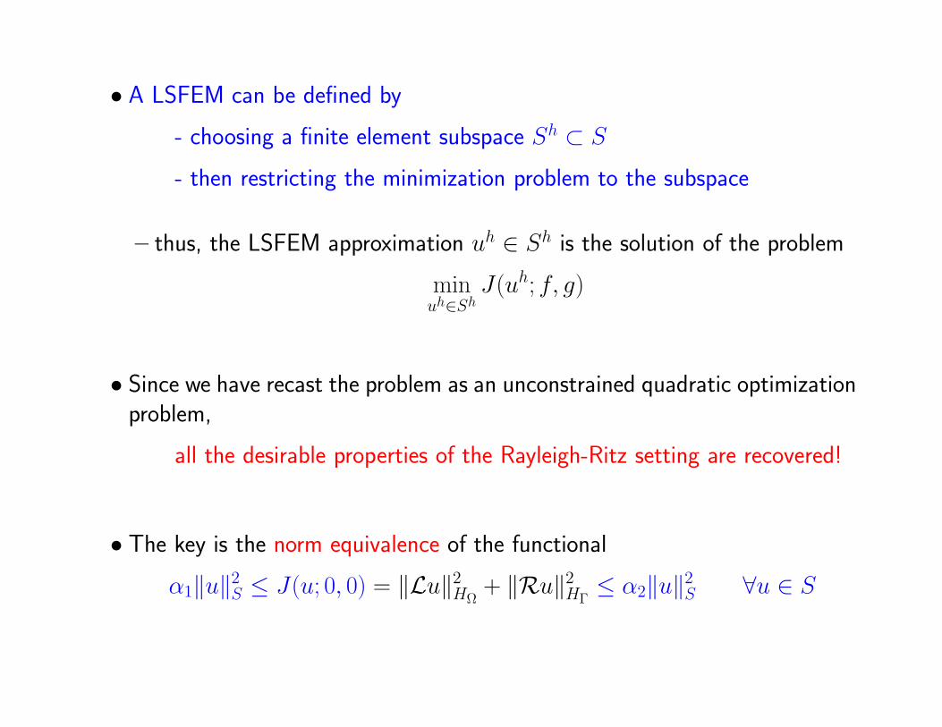
• A LSFEM can be defined by

- choosing a finite element subspace Sh ⊂ S

- then restricting the minimization problem to the subspace

– thus, the LSFEM approximation uh ∈ Sh is the solution of the problem

minuh∈Sh

J(uh; f, g)

• Since we have recast the problem as an unconstrained quadratic optimizationproblem,

all the desirable properties of the Rayleigh-Ritz setting are recovered!

• The key is the norm equivalence of the functional

α1‖u‖2S ≤ J(u; 0, 0) = ‖Lu‖2HΩ

+ ‖Ru‖2HΓ≤ α2‖u‖

2S ∀u ∈ S

• This is not the whole story: additional practicality criteria should be met

A. bases are easily constructed

B. linear systems are easily assembled

C. linear systems are relatively well conditioned

• Two keys to practicality

– use first-order system form of PDEs

– use L2 norms in the functional

• The choices (operators and spaces) that go into defining the straightforwardLSFEM are often in conflict with practicality

– i.e., there is often a conflict between norm equivalence and practicality

– this conflict has been largely resolved; see our upcoming Springer book

Today’s talk

•We consider mixed and least-squares finite element methods for the first-order system

u +∇φ = 0 and ∇ · u = f

which, of course, is equivalent to the Poisson equation

−∆φ = f

• This is a prototype for more general elliptic equations and Darcy flows

• Reasons for considering the first-order formulation include

– the flux variable u is often the primary variable of interest

– it may be easier to apply Dirichlet boundary conditions

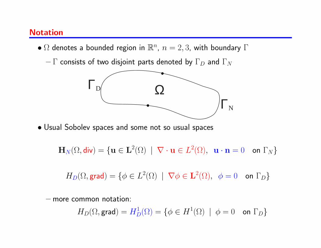
Notation

• Ω denotes a bounded region in Rn, n = 2, 3, with boundary Γ

– Γ consists of two disjoint parts denoted by ΓD and ΓN

ΩΓD

ΓN

• Usual Sobolev spaces and some not so usual spaces

HN(Ω, div) = u ∈ L2(Ω) | ∇ · u ∈ L2(Ω), u · n = 0 on ΓN

HD(Ω, grad) = φ ∈ L2(Ω) | ∇φ ∈ L2(Ω), φ = 0 on ΓD

– more common notation:

HD(Ω, grad) = H1D(Ω) = φ ∈ H1(Ω) | φ = 0 on ΓD

• Norms

‖φ‖HN (Ω,div)

=(‖u‖20 + ‖∇ · u‖20

)1/2

for u ∈ HN(Ω, div)

‖u‖HD(Ω,grad)

=(‖φ‖20 + ‖∇φ‖20

)1/2

for φ ∈ HD(Ω, grad)

•We will also use the spaces

∇ ·(HN(Ω, div)

)= L2(Ω)

∇(HD(Ω, grad)

)= u ∈ L

2(Ω) | ∇ × u = 0 ⊂ L2(Ω)

•With γ ≥ 0 a given function belonging to L∞(Ω), we will refer to theproblem

−∆φ + γφ = f in Ω, φ = 0 on ΓD, and ∂φ/∂n = 0 on ΓN

as the Poisson problem

THE GENERALIZED DIRICHLET AND KELVIN PRINCIPLES

• The Dirichlet and Kelvin principles arise in a variety of applications

•Mathematically, they provide two variational formulations for the Poissonproblem

• They also form the basis for defining mixed Galerkin finite element methodsfor approximations of the solution of the Poisson problem

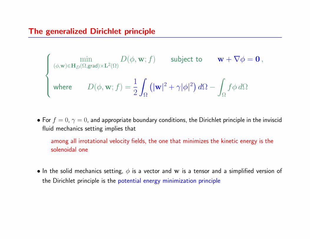
The generalized Dirichlet principle

min(φ,w)∈HD(Ω,grad)×L2(Ω)

D(φ,w; f) subject to w +∇φ = 0 ,

where D(φ,w; f) =1

2

∫

Ω

(|w|2 + γ|φ|2

)dΩ−

∫

Ω

fφ dΩ

• For f = 0, γ = 0, and appropriate boundary conditions, the Dirichlet principle in the inviscid

fluid mechanics setting implies that

among all irrotational velocity fields, the one that minimizes the kinetic energy is the

solenoidal one

• In the solid mechanics setting, φ is a vector and w is a tensor and a simplified version of

the Dirichlet principle is the potential energy minimization principle

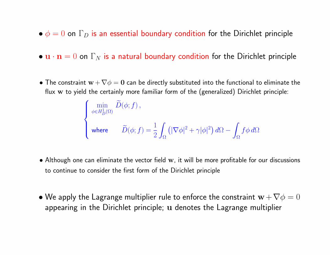
• φ = 0 on ΓD is an essential boundary condition for the Dirichlet principle

• u · n = 0 on ΓN is a natural boundary condition for the Dirichlet principle

• The constraint w+∇φ = 0 can be directly substituted into the functional to eliminate the

flux w to yield the certainly more familiar form of the (generalized) Dirichlet principle:

minφ∈H1

D(Ω)

D(φ; f) ,

where D(φ; f) =1

2

∫

Ω

(|∇φ|2 + γ|φ|2

)dΩ−

∫

Ω

fφ dΩ

• Although one can eliminate the vector field w, it will be more profitable for our discussions

to continue to consider the first form of the Dirichlet principle

•We apply the Lagrange multiplier rule to enforce the constraint w+∇φ = 0appearing in the Dirichlet principle; u denotes the Lagrange multiplier

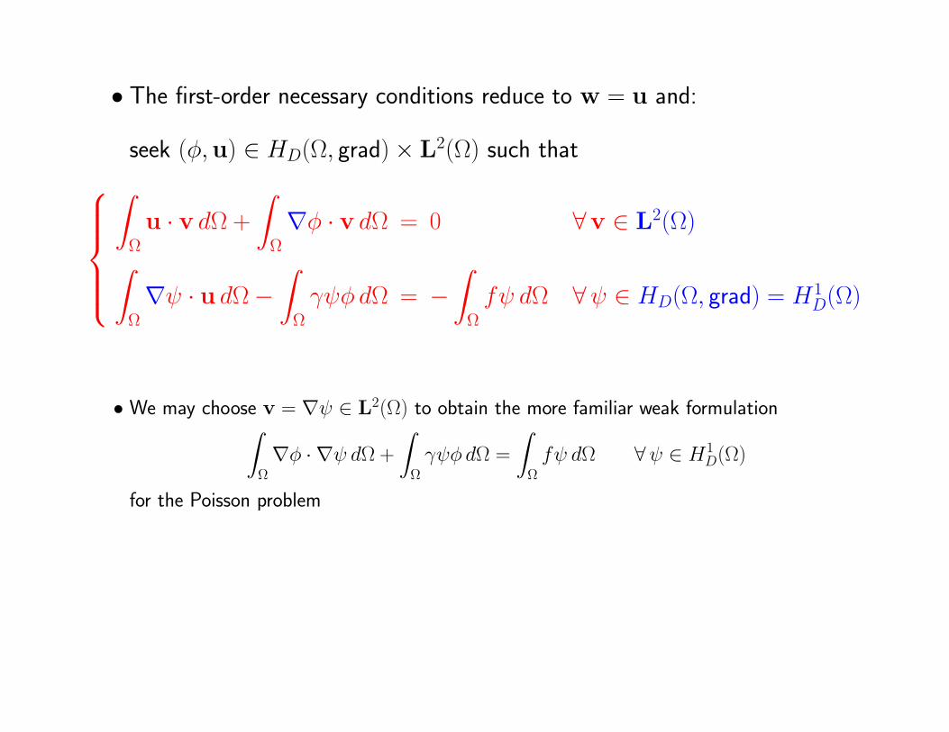
• The first-order necessary conditions reduce to w = u and:

seek (φ,u) ∈ HD(Ω, grad)× L2(Ω) such that

∫

Ω

u · v dΩ +

∫

Ω

∇φ · v dΩ = 0 ∀v ∈ L2(Ω)

∫

Ω

∇ψ · u dΩ−

∫

Ω

γψφ dΩ = −

∫

Ω

fψ dΩ ∀ψ ∈ HD(Ω, grad) = H1D(Ω)

• We may choose v = ∇ψ ∈ L2(Ω) to obtain the more familiar weak formulation

∫

Ω

∇φ · ∇ψ dΩ +

∫

Ω

γψφ dΩ =

∫

Ω

fψ dΩ ∀ψ ∈ H1D(Ω)

for the Poisson problem

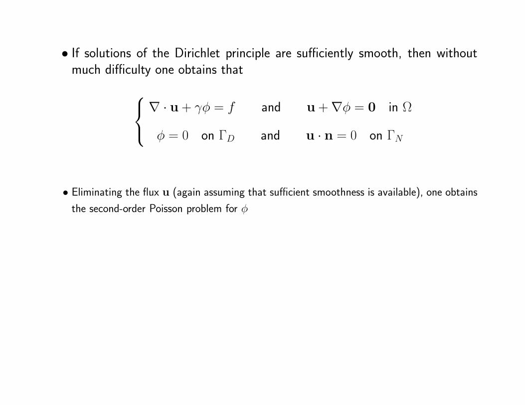
• If solutions of the Dirichlet principle are sufficiently smooth, then withoutmuch difficulty one obtains that

∇ · u + γφ = f and u +∇φ = 0 in Ω

φ = 0 on ΓD and u · n = 0 on ΓN

• Eliminating the flux u (again assuming that sufficient smoothness is available), one obtains

the second-order Poisson problem for φ

The generalized Kelvin principle

min(u,λ)∈HN(Ω,div)×L2(Ω)

K(λ,v) subject to ∇ · u + γλ = f ,

where K(λ,u) =1

2

∫

Ω

(|u|2 + γ|λ|2

)dΩ

• For f = 0, γ = 0, and appropriate boundary condition, the Kelvin principle for inviscid

flows implies that

among all incompressible velocity fields, the one that minimizes the kinetic energy is

irrotational

• In structural mechanics (with u is a tensor and λ is a vector), a simplified version of the

Kelvin principle is known as the minimum complimentary energy principle

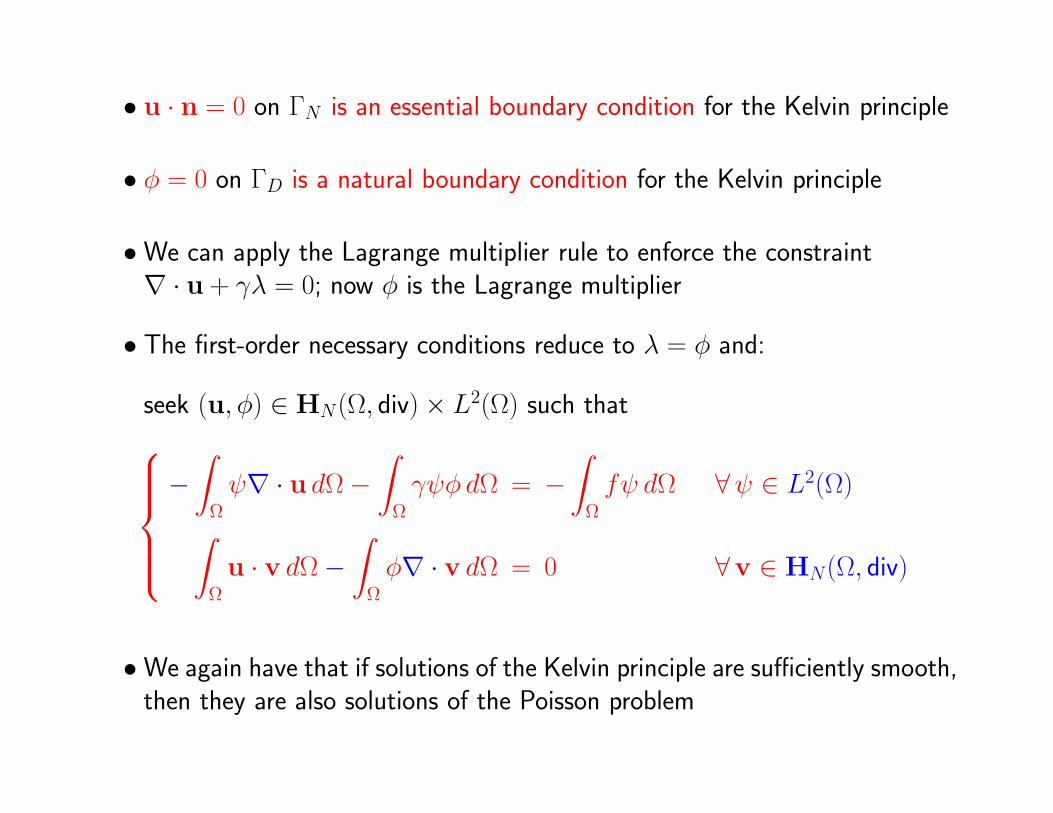
• u · n = 0 on ΓN is an essential boundary condition for the Kelvin principle

• φ = 0 on ΓD is a natural boundary condition for the Kelvin principle

•We can apply the Lagrange multiplier rule to enforce the constraint∇ · u + γλ = 0; now φ is the Lagrange multiplier

• The first-order necessary conditions reduce to λ = φ and:

seek (u, φ) ∈ HN(Ω, div)× L2(Ω) such that

−

∫

Ω

ψ∇ · u dΩ−

∫

Ω

γψφ dΩ = −

∫

Ω

fψ dΩ ∀ψ ∈ L2(Ω)

∫

Ω

u · v dΩ−

∫

Ω

φ∇ · v dΩ = 0 ∀v ∈ HN(Ω, div)

•We again have that if solutions of the Kelvin principle are sufficiently smooth,then they are also solutions of the Poisson problem

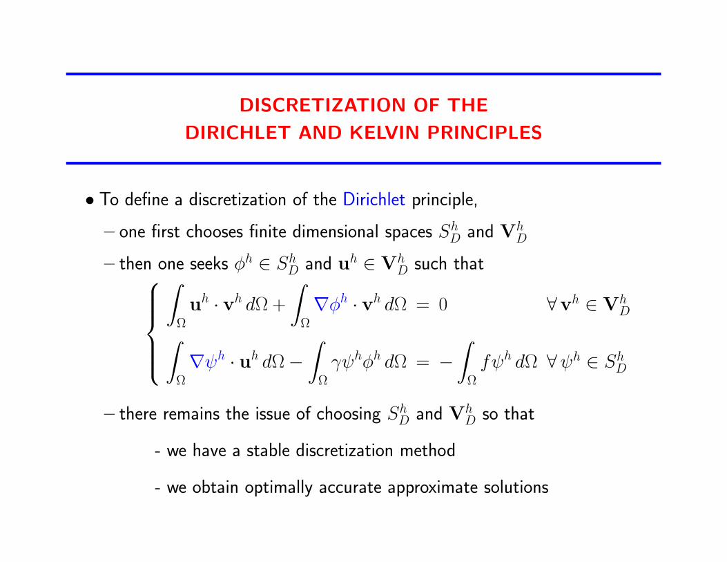
DISCRETIZATION OF THE

DIRICHLET AND KELVIN PRINCIPLES

• To define a discretization of the Dirichlet principle,

– one first chooses finite dimensional spaces ShD and VhD

– then one seeks φh ∈ ShD and uh ∈ V

hD such that

∫

Ω

uh · vh dΩ +

∫

Ω

∇φh · vh dΩ = 0 ∀vh ∈ V

hD

∫

Ω

∇ψh · uh dΩ−

∫

Ω

γψhφh dΩ = −

∫

Ω

fψh dΩ ∀ψh ∈ ShD

– there remains the issue of choosing ShD and VhD so that

- we have a stable discretization method

- we obtain optimally accurate approximate solutions

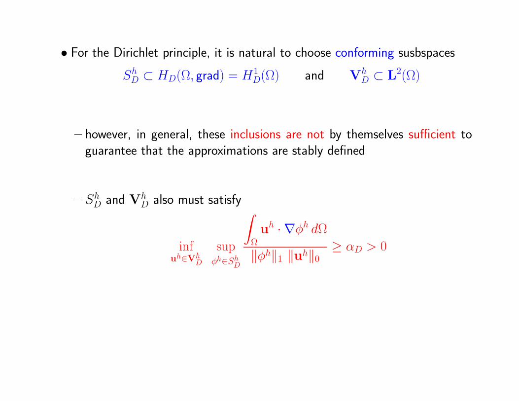
• For the Dirichlet principle, it is natural to choose conforming susbspaces

ShD ⊂ HD(Ω, grad) = H1D(Ω) and V

hD ⊂ L

2(Ω)

– however, in general, these inclusions are not by themselves sufficient toguarantee that the approximations are stably defined

– ShD and VhD also must satisfy

infuh∈Vh

D

supφh∈ShD

∫

Ω

uh · ∇φh dΩ

‖φh‖1 ‖uh‖0≥ αD > 0

• To define a discretization of the Kelvin principle,

– one first chooses finite dimensional spaces VhK and ShK

– then one seeks uh ∈ V

hK and φh ∈ ShK such that

∫

Ω

uh · vh dΩ−

∫

Ω

φh∇ · vh dΩ = 0 ∀vh ∈ V

hK

∫

Ω

ψh∇ · uh dΩ +

∫

Ω

γψhφh dΩ =

∫

Ω

fψh dΩ ∀ψh ∈ ShK

– there again remains the issue of choosing VhK and ShK so that

- we have a stable discretization method

- we obtain optimally accurate approximate solutions

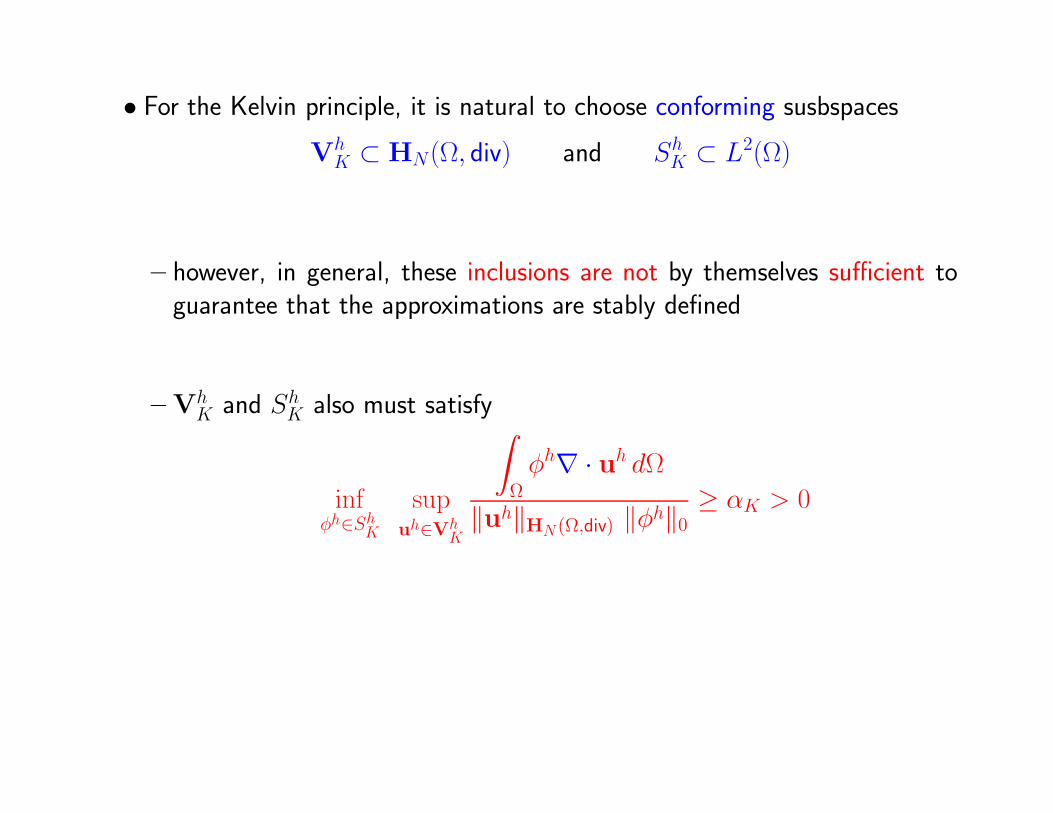
• For the Kelvin principle, it is natural to choose conforming susbspaces

VhK ⊂ HN(Ω, div) and ShK ⊂ L2(Ω)

– however, in general, these inclusions are not by themselves sufficient toguarantee that the approximations are stably defined

– VhK and ShK also must satisfy

infφh∈ShK

supuh∈Vh

K

∫

Ω

φh∇ · uh dΩ

‖uh‖HN (Ω,div) ‖φh‖0≥ αK > 0

Stable finite element methods for the Dirichlet principle

• Let

Th denote a simplicial triangulation of Ω into elements

K denote an element of Th

Pk(K) denote the space of all polynomials of degree less than or equal to kdefined on K

• For the Dirichlet principle, we choose

ShD =W0m = ψ ∈ C0(Ω) | ψ|K ∈ Pm(K)

VhD =W1

m = ∇(W0

m

)

• The space W01 restricted to an element

– the degrees of freedom are the nodal values

• The space W11 = ∇(W0

1 ) restricted to an element

– the degrees of freedom are vectors tangent to the edges

• It can be shown that if φ ∈ Hm+1(Ω) ∩H1D(Ω), then

‖φ− φh‖0 ≤ Chm+1‖φ‖m+1

‖u− uh‖0 = ‖∇(φ− φh)‖0 ≤ Chm‖φ‖m+1

• Note that, sinceW1m ≡ ∇(W0

m), even at the discrete level, we may again eliminate the flux

approximation to obtain the equivalent discrete problem∫

Ω

∇φh · ∇ψh dΩ +

∫

Ω

γψhφh dΩ =

∫

Ω

fψh dΩ ∀ψ ∈ W0m

that we recognize as the standard Galerkin discretization of the second-order Poisson problem

– in fact, solutions of the first and second-order problems are identical

– in this way we see that for discretizations of the Dirichlet principle, therequired inf-sup condition is completely benign

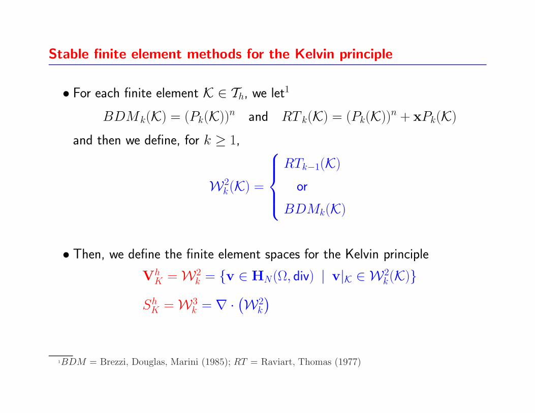
Stable finite element methods for the Kelvin principle

• For each finite element K ∈ Th, we let1

BDMk(K) = (Pk(K))n and RT k(K) = (Pk(K))n + xPk(K)

and then we define, for k ≥ 1,

W2k(K) =

RTk−1(K)

or

BDMk(K)

• Then, we define the finite element spaces for the Kelvin principle

VhK =W2

k = v ∈ HN(Ω, div) | v|K ∈ W2k(K)

ShK =W3k = ∇ ·

(W2

k

)

1BDM = Brezzi, Douglas, Marini (1985); RT = Raviart, Thomas (1977)

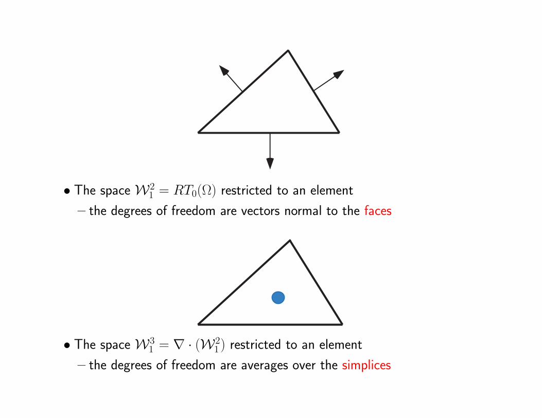
• The space W21 = RT0(Ω) restricted to an element

– the degrees of freedom are vectors normal to the faces

• The space W31 = ∇ · (W2

1 ) restricted to an element

– the degrees of freedom are averages over the simplices

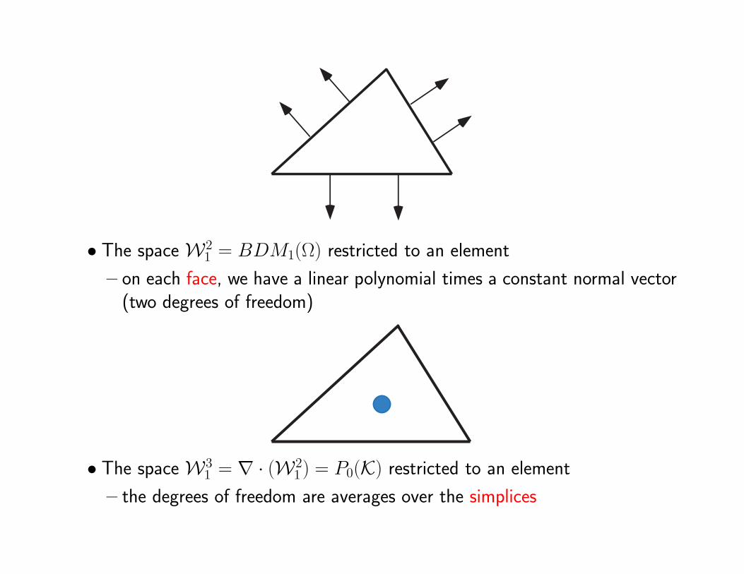
• The space W21 = BDM1(Ω) restricted to an element

– on each face, we have a linear polynomial times a constant normal vector(two degrees of freedom)

• The space W31 = ∇ · (W2

1 ) = P0(K) restricted to an element

– the degrees of freedom are averages over the simplices

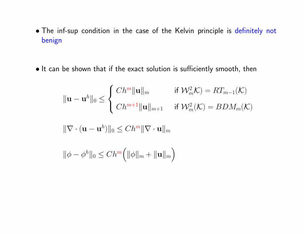
• The inf-sup condition in the case of the Kelvin principle is definitely notbenign

• It can be shown that if the exact solution is sufficiently smooth, then

‖u− uh‖0 ≤

Chm‖u‖m if W2

mK) = RTm−1(K)

Chm+1‖u‖m+1 if W2m(K) = BDMm(K)

‖∇ · (u− uh)‖0 ≤ Chm‖∇ · u‖m

‖φ− φh‖0 ≤ Chm(‖φ‖m + ‖u‖m

)

• It is important to note that

if one uses C0(Ω) finite element spaces for both the scalar and the flux,

then the discrete Dirichlet and Kelvin problems are identical

– it is well known that this leads to unstable approximations so that onecannot use (without introducing a stabilization techniques) such pairs offinite element spaces in mixed methods derived from either the Dirichletor Kelvin principles

– in particular, for such methods, one cannot use the same finite elementspace for approximating both the scalar and flux variables

• In passing, we note that both the discrete Dirichlet and Kelvin are, in general,symmetric and indefinite

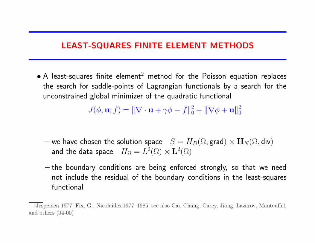
LEAST-SQUARES FINITE ELEMENT METHODS

• A least-squares finite element2 method for the Poisson equation replacesthe search for saddle-points of Lagrangian functionals by a search for theunconstrained global minimizer of the quadratic functional

J(φ,u; f) = ‖∇ · u + γφ− f‖20 + ‖∇φ + u‖20

– we have chosen the solution space S = HD(Ω, grad)×HN(Ω, div)and the data space HΩ = L2(Ω)× L

2(Ω)

– the boundary conditions are being enforced strongly, so that we neednot include the residual of the boundary conditions in the least-squaresfunctional

2Jespersen 1977; Fix, G., Nicolaides 1977–1985; see also Cai, Chang, Carey, Jiang, Lazarov, Manteuffel,

and others (94-00)

• A least-squares variational principle is therefore given by

min(φ,u)∈HD(Ω,grad)×HN (Ω,div)

J(φ,u; f)

• Its solution minimizes the L2-norm of the residuals of the first-order system

∇ · u + γφ = f and u +∇φ = 0

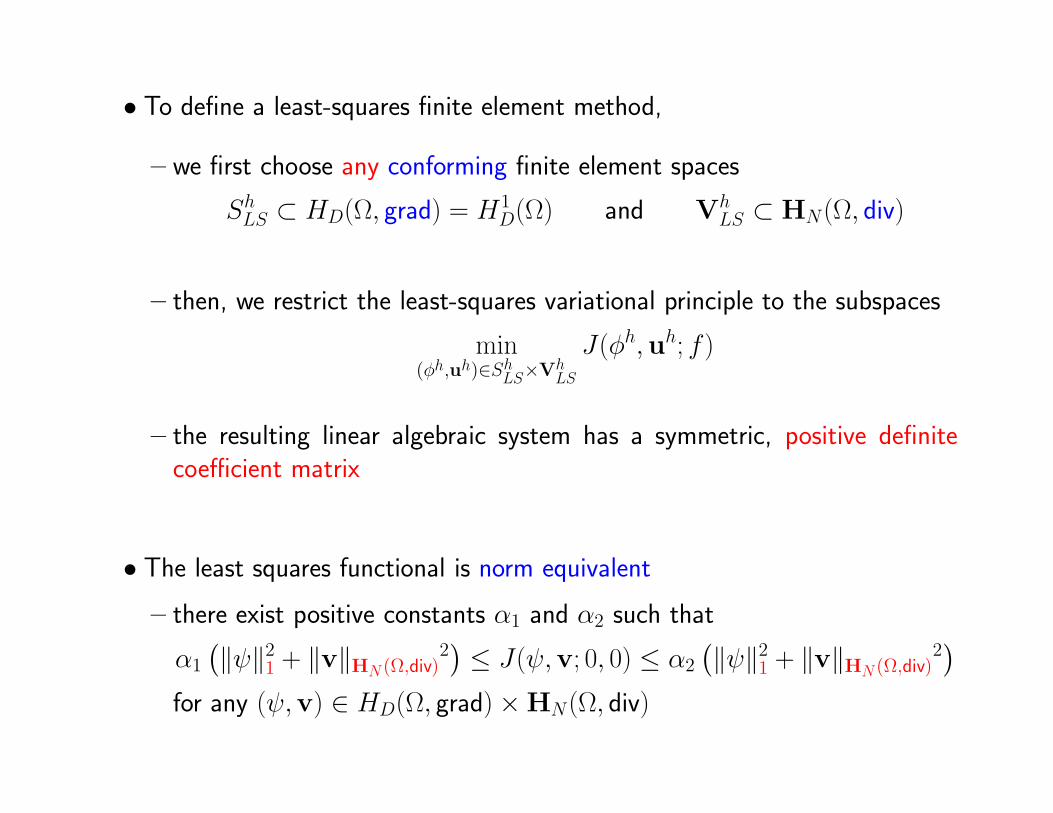
• To define a least-squares finite element method,

– we first choose any conforming finite element spaces

ShLS ⊂ HD(Ω, grad) = H1D(Ω) and V

hLS ⊂ HN(Ω, div)

– then, we restrict the least-squares variational principle to the subspaces

min(φh,uh)∈ShLS×Vh

LS

J(φh,uh; f)

– the resulting linear algebraic system has a symmetric, positive definitecoefficient matrix

• The least squares functional is norm equivalent

– there exist positive constants α1 and α2 such that

α1

(‖ψ‖21 + ‖v‖HN (Ω,div)

2)≤ J(ψ,v; 0, 0) ≤ α2

(‖ψ‖21 + ‖v‖HN (Ω,div)

2)

for any (ψ,v) ∈ HD(Ω, grad)×HN(Ω, div)

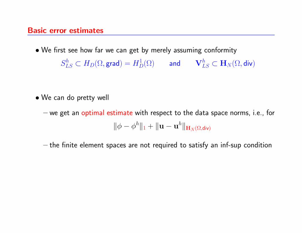
Basic error estimates

•We first see how far we can get by merely assuming conformity

ShLS ⊂ HD(Ω, grad) = H1D(Ω) and V

hLS ⊂ HN(Ω, div)

•We can do pretty well

– we get an optimal estimate with respect to the data space norms, i.e., for

‖φ− φh‖1 + ‖u− uh‖HN (Ω,div)

– the finite element spaces are not required to satisfy an inf-sup condition

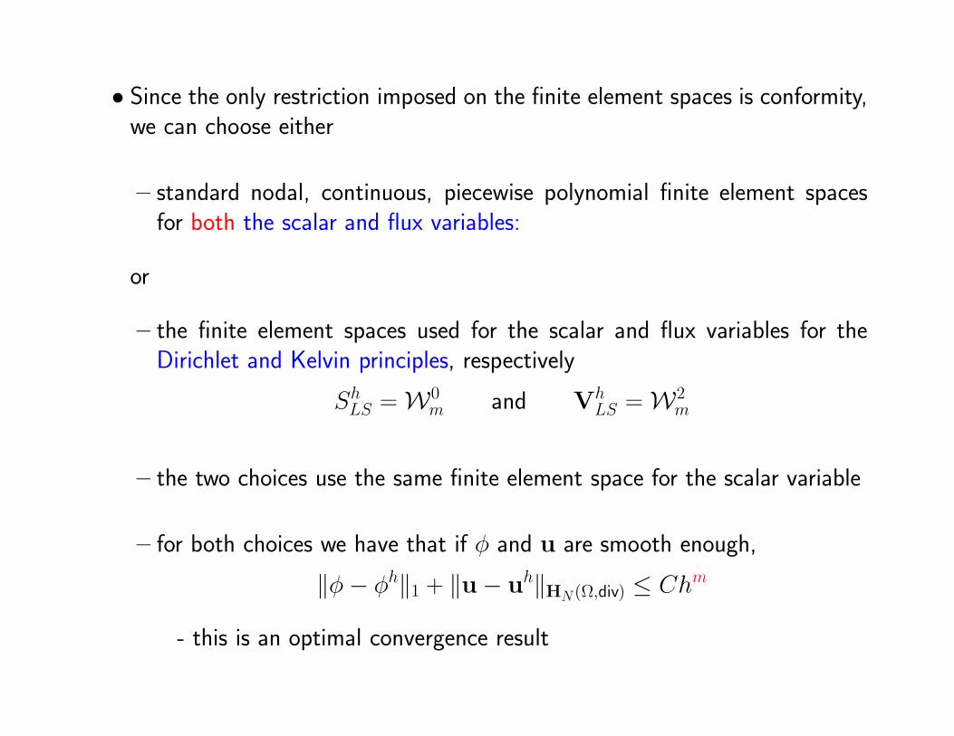
• Since the only restriction imposed on the finite element spaces is conformity,we can choose either

– standard nodal, continuous, piecewise polynomial finite element spacesfor both the scalar and flux variables:

or

– the finite element spaces used for the scalar and flux variables for theDirichlet and Kelvin principles, respectively

ShLS =W0m and V

hLS =W2

m

– the two choices use the same finite element space for the scalar variable

– for both choices we have that if φ and u are smooth enough,

‖φ− φh‖1 + ‖u− uh‖HN (Ω,div) ≤ Chm

- this is an optimal convergence result

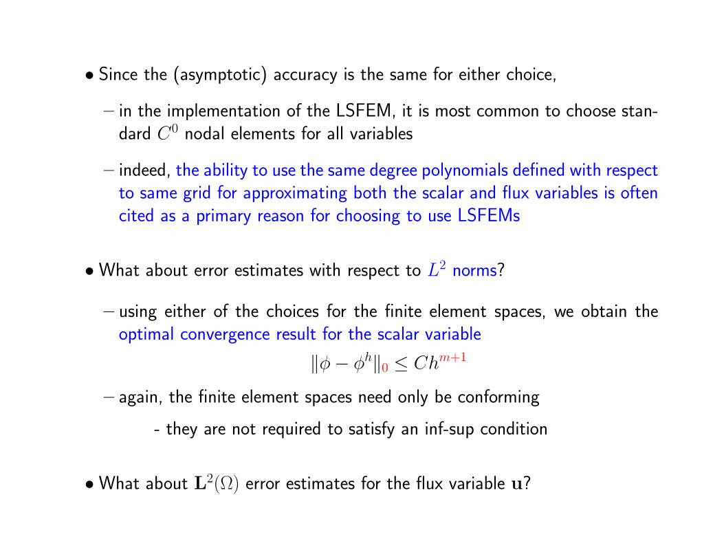
• Since the (asymptotic) accuracy is the same for either choice,

– in the implementation of the LSFEM, it is most common to choose stan-dard C0 nodal elements for all variables

– indeed, the ability to use the same degree polynomials defined with respectto same grid for approximating both the scalar and flux variables is oftencited as a primary reason for choosing to use LSFEMs

•What about error estimates with respect to L2 norms?

– using either of the choices for the finite element spaces, we obtain theoptimal convergence result for the scalar variable

‖φ− φh‖0 ≤ Chm+1

– again, the finite element spaces need only be conforming

- they are not required to satisfy an inf-sup condition

•What about L2(Ω) error estimates for the flux variable u?

L2 error estimates for the flux u

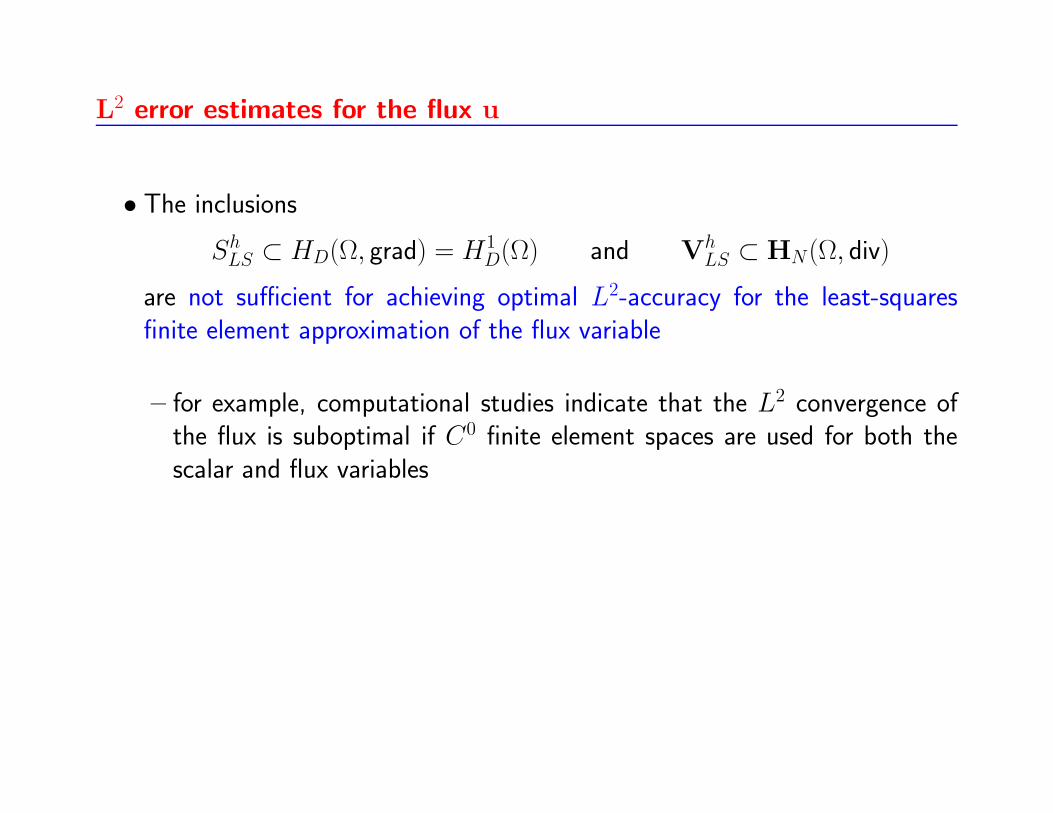
• The inclusions

ShLS ⊂ HD(Ω, grad) = H1D(Ω) and V

hLS ⊂ HN(Ω, div)

are not sufficient for achieving optimal L2-accuracy for the least-squaresfinite element approximation of the flux variable

– for example, computational studies indicate that the L2 convergence ofthe flux is suboptimal if C0 finite element spaces are used for both thescalar and flux variables

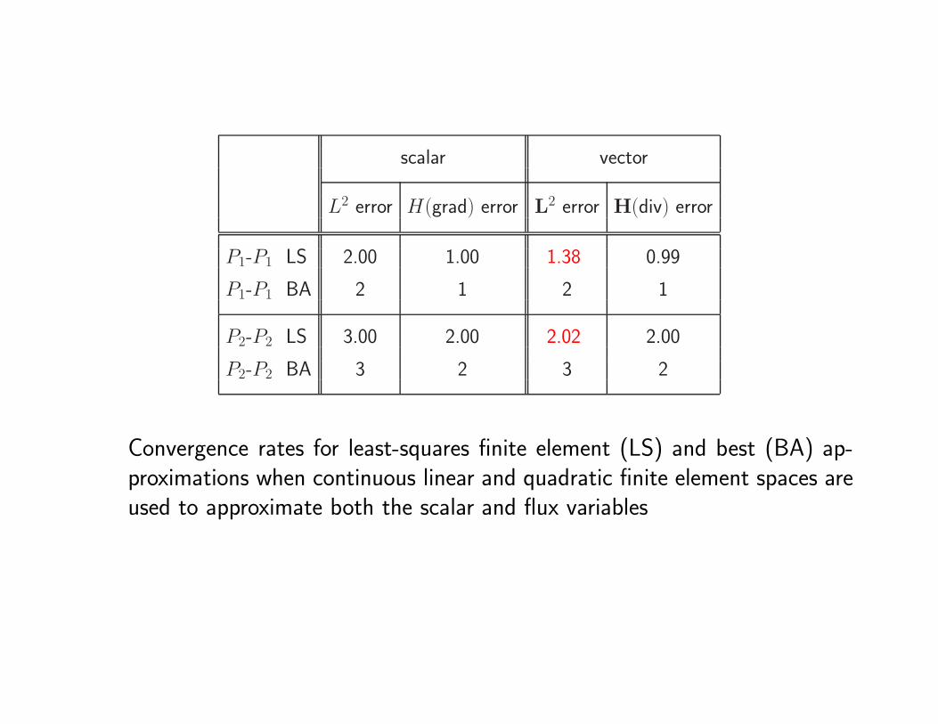
scalar vector

L2 error H(grad) error L2 error H(div) error

P1-P1 LS 2.00 1.00 1.38 0.99

P1-P1 BA 2 1 2 1

P2-P2 LS 3.00 2.00 2.02 2.00

P2-P2 BA 3 2 3 2

Convergence rates for least-squares finite element (LS) and best (BA) ap-proximations when continuous linear and quadratic finite element spaces areused to approximate both the scalar and flux variables

• However, if

ShLS =W0k ⊂ HD(Ω, grad) = H1

D(Ω) and VhLS =W2

k ⊂ HN(Ω, div)

i.e., if

- the finite element space for the scalar is a stable space forthe Dirichlet principle

- the finite element space for the flux is a stable space forthe Kelvin principle

then, optimal L2(Ω) error estimates for both the scalar and flux variables areobtained

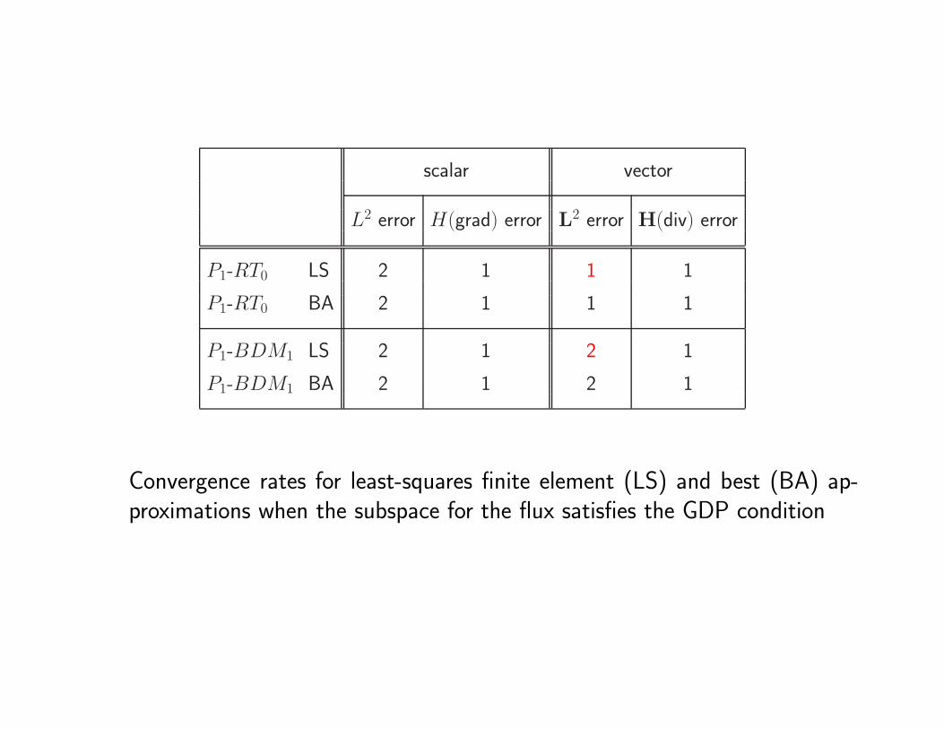
scalar vector

L2 error H(grad) error L2 error H(div) error

P1-RT0 LS 2 1 1 1

P1-RT0 BA 2 1 1 1

P1-BDM1 LS 2 1 2 1

P1-BDM1 BA 2 1 2 1

Convergence rates for least-squares finite element (LS) and best (BA) ap-proximations when the subspace for the flux satisfies the GDP condition

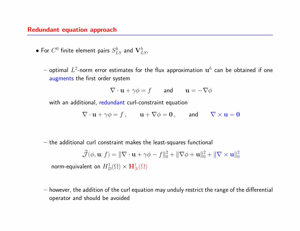
Redundant equation approach

• For C0 finite element pairs ShLS and VhLS,

– optimal L2-norm error estimates for the flux approximation uh can be obtained if one

augments the first order system

∇ · u + γφ = f and u = −∇φ

with an additional, redundant curl-constraint equation

∇ · u + γφ = f , u +∇φ = 0 , and ∇× u = 0

– the additional curl constraint makes the least-squares functional

J (φ,u; f) = ‖∇ · u + γφ− f‖20 + ‖∇φ+ u‖20 + ‖∇ × u‖20

norm-equivalent on H1D(Ω)×H

1N(Ω)

– however, the addition of the curl equation may unduly restrict the range of the differential

operator and should be avoided

LEAST-SQUARES AND MIXED FINITE ELEMENT METHODS

•We have seen that a least-squares finite element method implemented usingequal-order C0 finite element spaces

– approximates the scalar variable with the same accuracy as a mixed methodfor the Dirichlet principle

– however, the approximation properties of the Kelvin principle are onlypartially inherited ⇒ the accuracy in the approximation of

- the divergence of the flux is recovered

- but not that for the flux itself

– perhaps this this is not surprising since C0 elements

- provide stable discretization for the scalar in the Dirichlet principle

- but not that for the flux in the Kelvin principle

• It seems that while least-squares minimization

– is stable enough to allow for the approximation of the scalar variable andthe flux by equal-order C0 finite element spaces,

– it cannot completely recover from the fact that such spaces are unstablefor the Kelvin principle

• The key observation is that a least-squares finite element method can inheritthe computational properties of both the Dirichlet and the Kelvin principles

– provided the scalar and flux variables are respectively approximated byfinite element spaces that are stable with respect to those two principles

– then, least-squares finite element solutions recover

- the accuracy of the Dirichlet principle for the scalar variable

- the accuracy of the Kelvin principle for the flux

• Thus, there seems to be some deep connections between mixed methods andleast-squares finite element methods

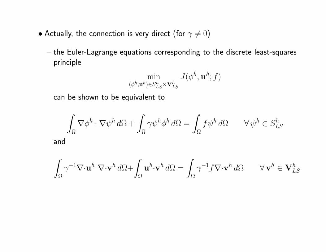
• Actually, the connection is very direct (for γ 6= 0)

– the Euler-Lagrange equations corresponding to the discrete least-squaresprinciple

min(φh,uh)∈ShLS×Vh

LS

J(φh,uh; f)

can be shown to be equivalent to

∫

Ω

∇φh · ∇ψh dΩ +

∫

Ω

γψhφh dΩ =

∫

Ω

fψh dΩ ∀ψh ∈ ShLS

and

∫

Ω

γ−1∇·uh ∇·vh dΩ+

∫

Ω

uh·vh dΩ =

∫

Ω

γ−1f∇·vh dΩ ∀vh ∈ V

hLS

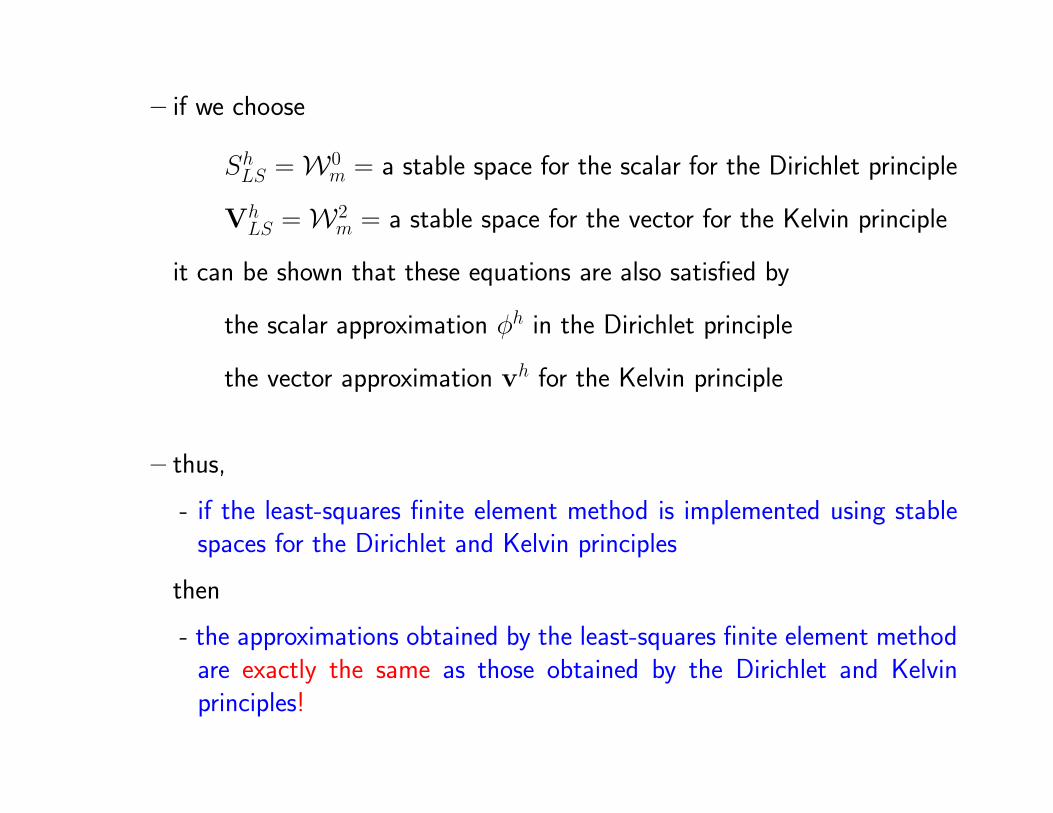
– if we choose

ShLS =W0m = a stable space for the scalar for the Dirichlet principle

VhLS =W2

m = a stable space for the vector for the Kelvin principle

it can be shown that these equations are also satisfied by

the scalar approximation φh in the Dirichlet principle

the vector approximation vh for the Kelvin principle

– thus,

- if the least-squares finite element method is implemented using stablespaces for the Dirichlet and Kelvin principles

then

- the approximations obtained by the least-squares finite element methodare exactly the same as those obtained by the Dirichlet and Kelvinprinciples!

• So, what is the advantage of LSFEMs over mixed Galerkin FEMs?

– one can recover the accuracy of the scalar variable in the Dirichlet principleand the vector variable in the Kelvin principle

- one does not have to choose which one to approximate better

– one can do this by solving a symmetric, positive definite matrix problem

• Of course, if one does not care about the optimal L2(Ω) accuracy of the

vector variable, then one can use equal-order interpolation for all variablesin the LSFEM

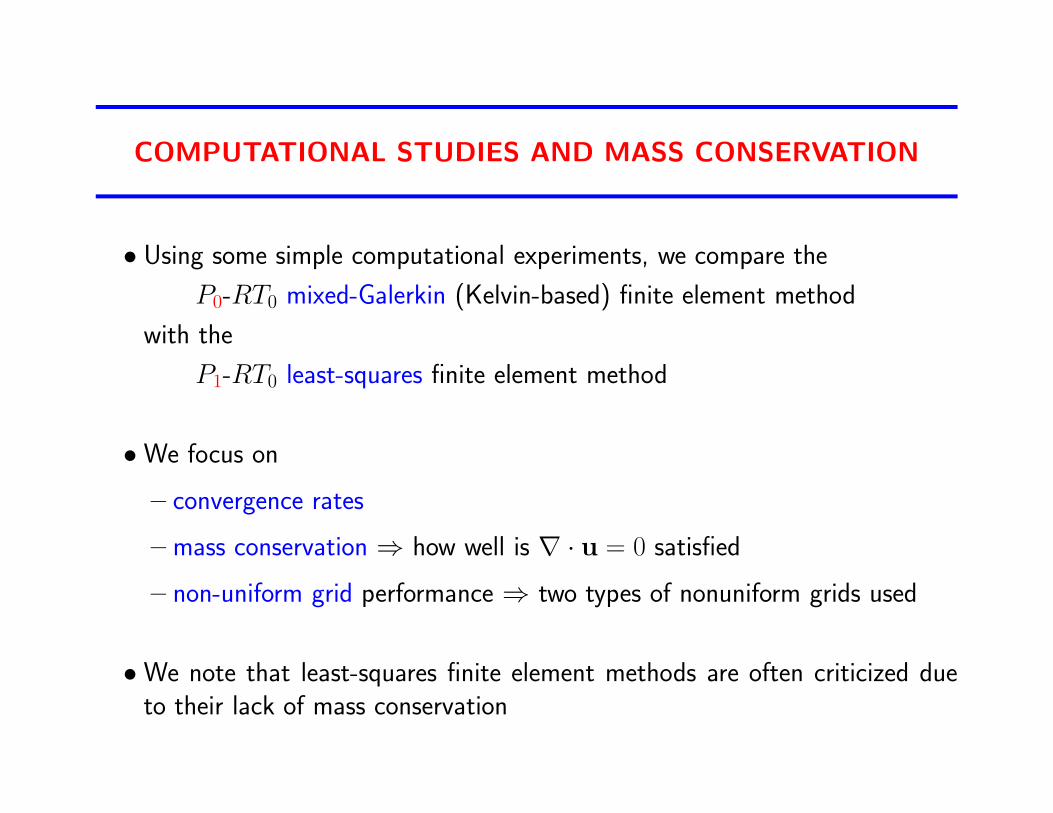
COMPUTATIONAL STUDIES AND MASS CONSERVATION

• Using some simple computational experiments, we compare the

P0-RT0 mixed-Galerkin (Kelvin-based) finite element method

with the

P1-RT0 least-squares finite element method

•We focus on

– convergence rates

– mass conservation ⇒ how well is ∇ · u = 0 satisfied

– non-uniform grid performance ⇒ two types of nonuniform grids used

•We note that least-squares finite element methods are often criticized dueto their lack of mass conservation

Non-uniform grids used in computational experiments

left: randomly perturbed grid

right: smooth, structured grid

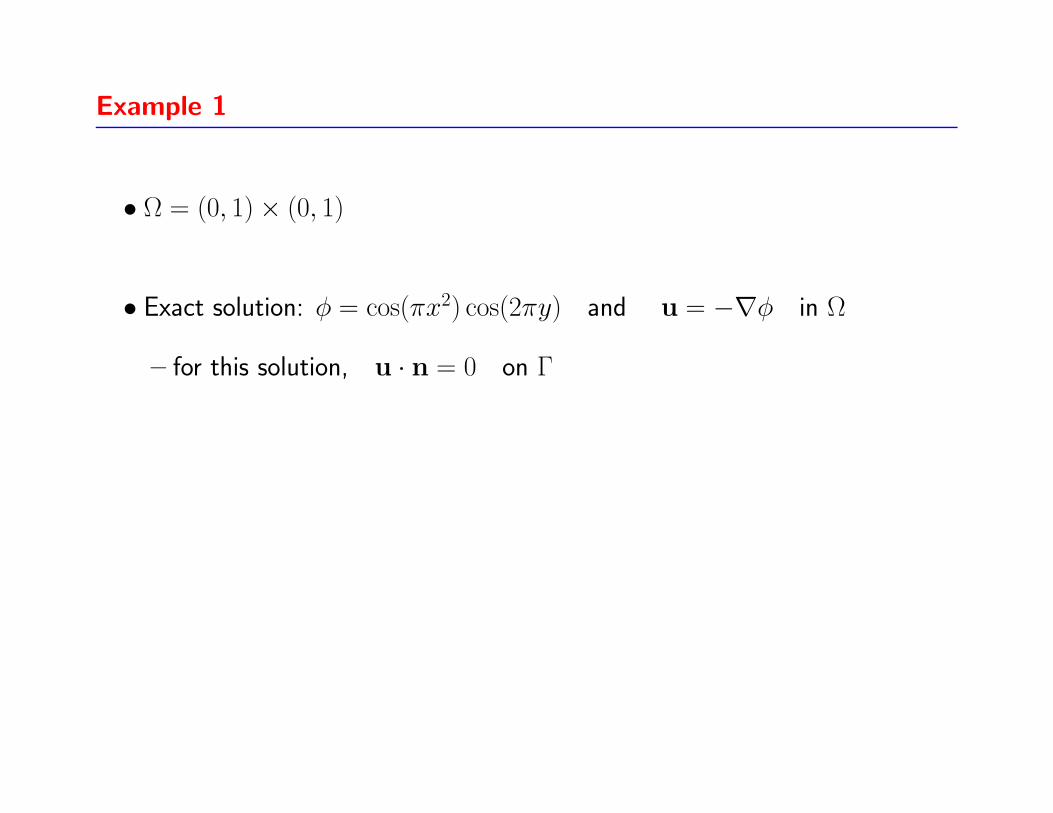
Example 1

• Ω = (0, 1)× (0, 1)

• Exact solution: φ = cos(πx2) cos(2πy) and u = −∇φ in Ω

– for this solution, u · n = 0 on Γ

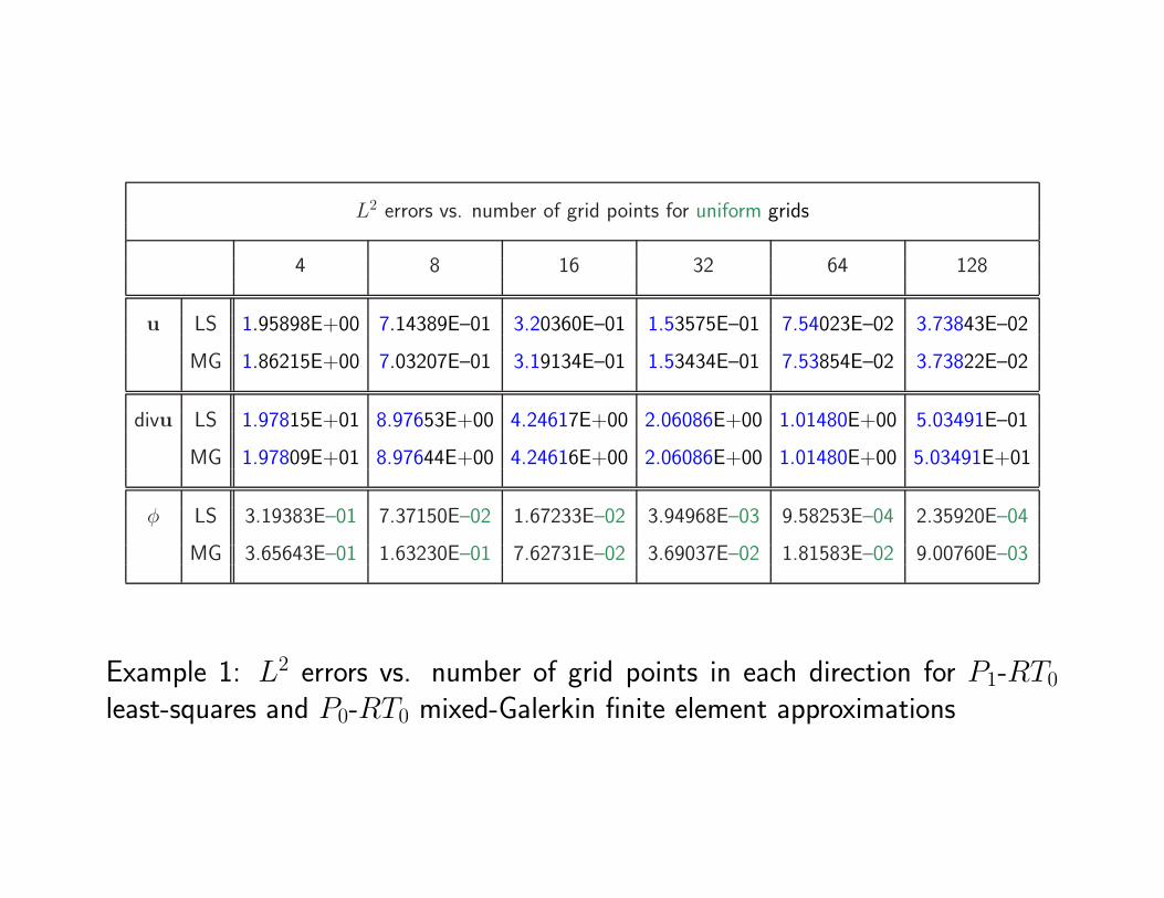
L2 errors vs. number of grid points for uniform grids

4 8 16 32 64 128

u LS 1.95898E+00 7.14389E–01 3.20360E–01 1.53575E–01 7.54023E–02 3.73843E–02

MG 1.86215E+00 7.03207E–01 3.19134E–01 1.53434E–01 7.53854E–02 3.73822E–02

divu LS 1.97815E+01 8.97653E+00 4.24617E+00 2.06086E+00 1.01480E+00 5.03491E–01

MG 1.97809E+01 8.97644E+00 4.24616E+00 2.06086E+00 1.01480E+00 5.03491E+01

φ LS 3.19383E–01 7.37150E–02 1.67233E–02 3.94968E–03 9.58253E–04 2.35920E–04

MG 3.65643E–01 1.63230E–01 7.62731E–02 3.69037E–02 1.81583E–02 9.00760E–03

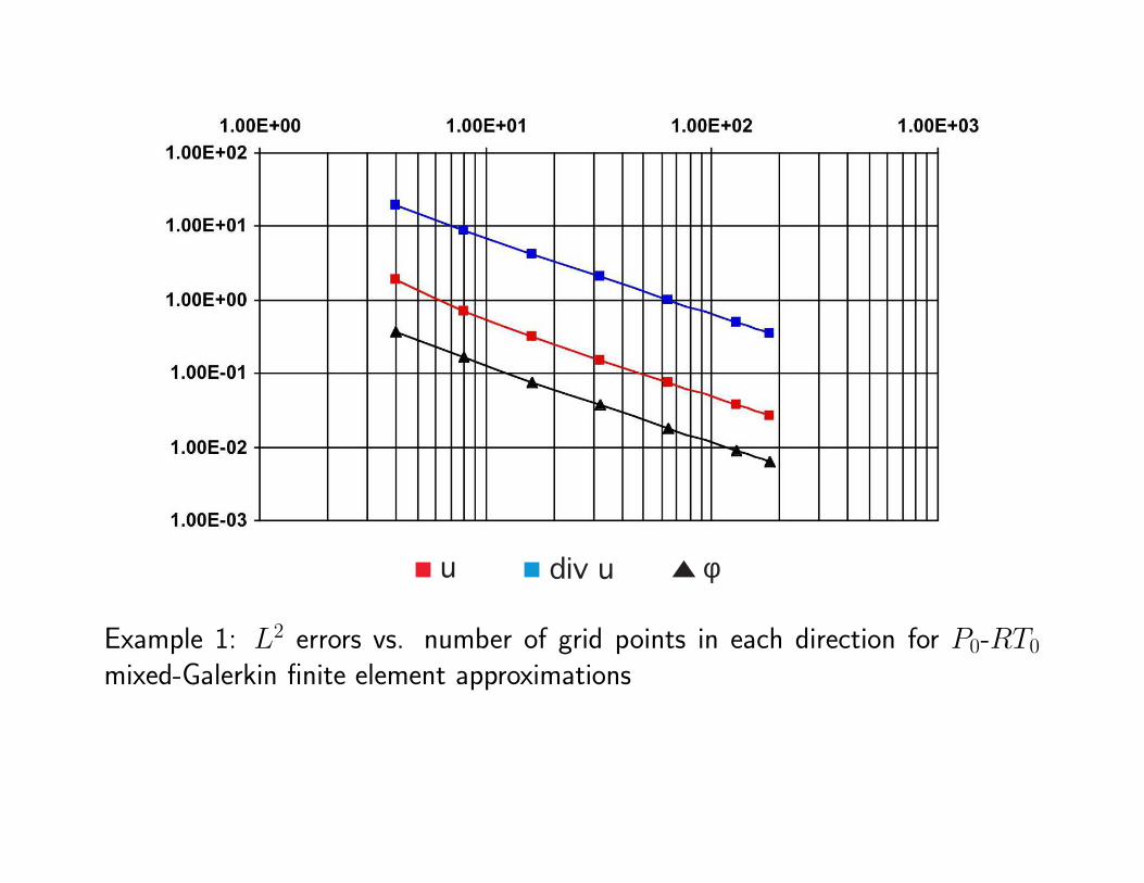
Example 1: L2 errors vs. number of grid points in each direction for P1-RT0

least-squares and P0-RT0 mixed-Galerkin finite element approximations

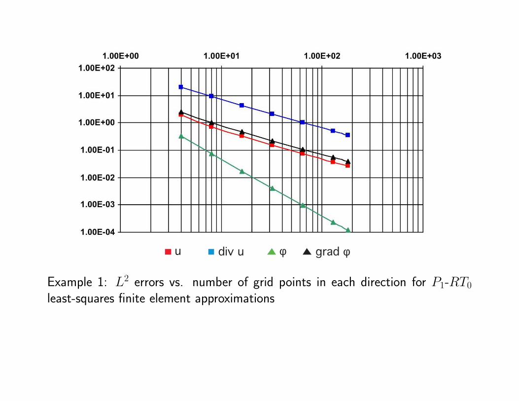
u div u φ grad φ

Example 1: L2 errors vs. number of grid points in each direction for P1-RT0

least-squares finite element approximations

u div u φ

Example 1: L2 errors vs. number of grid points in each direction for P0-RT0

mixed-Galerkin finite element approximations

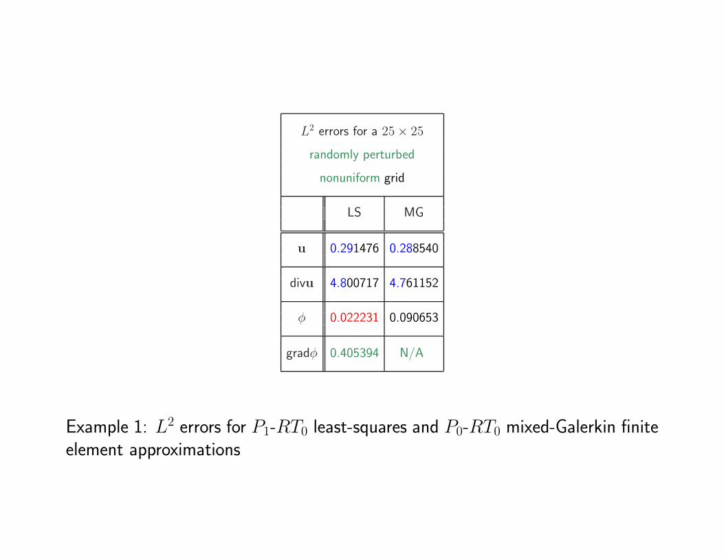
L2 errors for a 25× 25

randomly perturbed

nonuniform grid

LS MG

u 0.291476 0.288540

divu 4.800717 4.761152

φ 0.022231 0.090653

gradφ 0.405394 N/A

Example 1: L2 errors for P1-RT0 least-squares and P0-RT0 mixed-Galerkin finiteelement approximations

5 10 15 20 25

5

10

15

20

25

5 10 15 20 25

5

10

15

20

25

5 10 15 20 25

5

10

15

20

25

510

1520

25510152025

-4-2024

510

1520

25

510

1520

25510152025

-505

510

1520

25

510 1520

25510152025

-1-0.5

00.51

510 1520

25

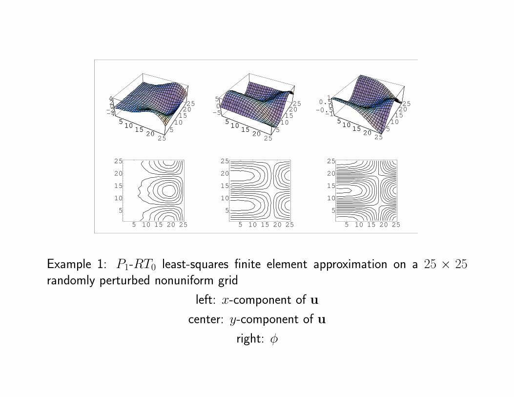
Example 1: P1-RT0 least-squares finite element approximation on a 25 × 25randomly perturbed nonuniform grid

left: x-component of u

center: y-component of u

right: φ

5 10 15 20 25

5

10

15

20

25

5 10 15 20 25

5

10

15

20

25

5 10 15 20 25

5

10

15

20

25

510

1520

25510152025

-4-2024

510

1520

25

510

1520

25510152025

-505

510

1520

25

510 1520

25510152025

-1-0.500.51

510 1520

25

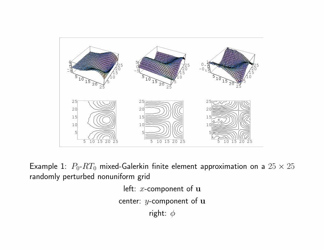
Example 1: P0-RT0 mixed-Galerkin finite element approximation on a 25 × 25randomly perturbed nonuniform grid

left: x-component of u

center: y-component of u

right: φ

L2 errors for a 25× 25

smooth, structured

nonuniform grid

LS MG

u 0.270278 0.269682

divu 3.58186 3.58185

φ 0.012129 0.064601

gradφ 0.387836 N/A

Example 1: L2 errors for P1-RT0 least-squares and P0-RT0 mixed-Galerkin finiteelement approximations

5 10 15 20 25

5

10

15

20

25

5 10 15 20 25

5

10

15

20

25

5 10 15 20 25

5

10

15

20

25

510

1520

25510152025

-4-2024

510

1520

25

510

1520

25510152025

-505

510

1520

25

510 1520

25510152025

-1-0.5

00.51

510 1520

25

Example 1: P1-RT0 least-squares finite element approximation on a 25 × 25smooth, structured nonuniform grid

left: x-component of u

center: y-component of u

right: φ

5 10 15 20 25

5

10

15

20

25

5 10 15 20 25

5

10

15

20

25

5 10 15 20 25

5

10

15

20

25

510

1520

25510152025

-4-2024

510

1520

25

510

1520

25510152025

-505

510

1520

25

510 1520

25510152025

-1-0.50

0.51

510 1520

25

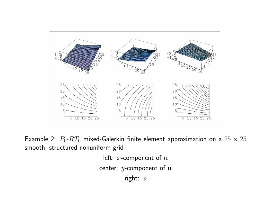
Example 1: P0-RT0 mixed-Galerkin finite element approximation on a 25 × 25smooth, structured nonuniform grid

left: x-component of u

center: y-component of u

right: φ

5 10 15 20 25

5

10

15

20

25

510

1520

25

5

10

15

2025

-1-0.5

00.51

510

1520

25

5 10 15 20 25

5

10

15

20

25

510

1520

25

5

10

15

20

25

-1

0

1

510

1520

25

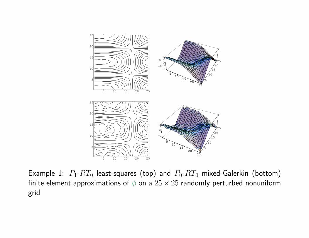
Example 1: P1-RT0 least-squares (top) and P0-RT0 mixed-Galerkin (bottom)finite element approximations of φ on a 25× 25 randomly perturbed nonuniformgrid

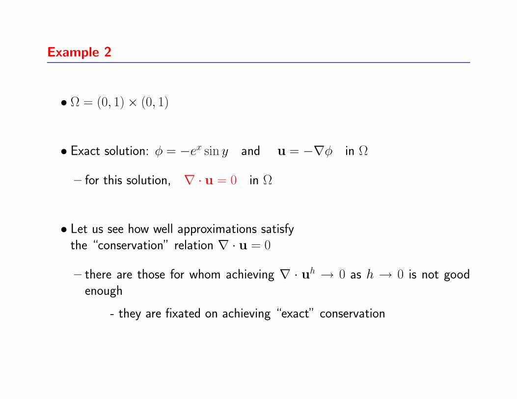
Example 2

• Ω = (0, 1)× (0, 1)

• Exact solution: φ = −ex sin y and u = −∇φ in Ω

– for this solution, ∇ · u = 0 in Ω

• Let us see how well approximations satisfythe “conservation” relation ∇ · u = 0

– there are those for whom achieving ∇ · uh → 0 as h → 0 is not goodenough

- they are fixated on achieving “exact” conservation

0 5 10 15 20 250

5

10

15

20

25

-4·10-7 -2·10-7 0 2·10-7 4·10-70

20

40

60

80

0 5 10 15 20 250

5

10

15

20

25

0 5·10-16 1·10-15 1.5·10-15 2·10-15 2.5·10-150

100

200

300

400

500

600

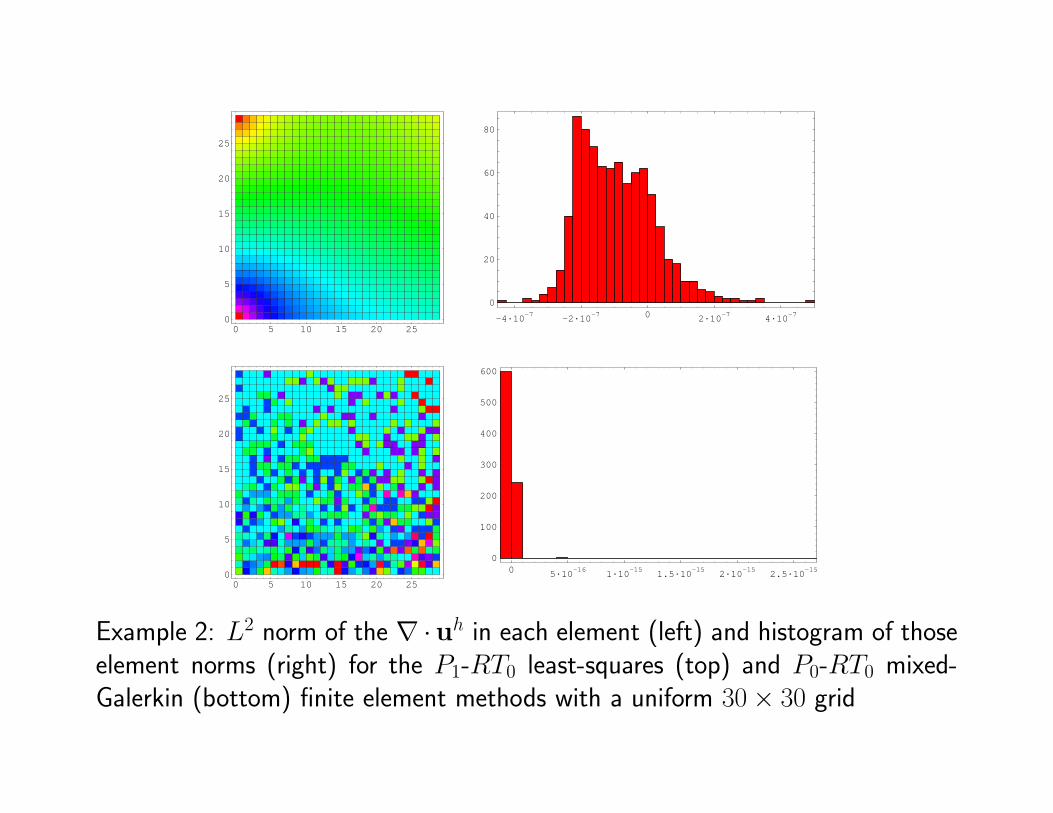
Example 2: L2 norm of the ∇ ·uh in each element (left) and histogram of thoseelement norms (right) for the P1-RT0 least-squares (top) and P0-RT0 mixed-Galerkin (bottom) finite element methods with a uniform 30× 30 grid

L2 errors for 30× 30 grids

u divu

uniform LS 0.214582E–01 0.123507E–03

MG 0.214581E–01 0.144627E–13

random LS 0.234284E–01 0.166878E–03

MG 0.235258E–01 0.665824E–14

Example 2: L2 errors for P1-RT0 least-squares and P0-RT0 mixed-Galerkin finiteelement approximations

• Although ‖∇ · uh‖0 is small for the least-squares approximation, it is notwithin round-off error of the exact relation ∇·u = 0 as is the mixed-Galerkinapproximation

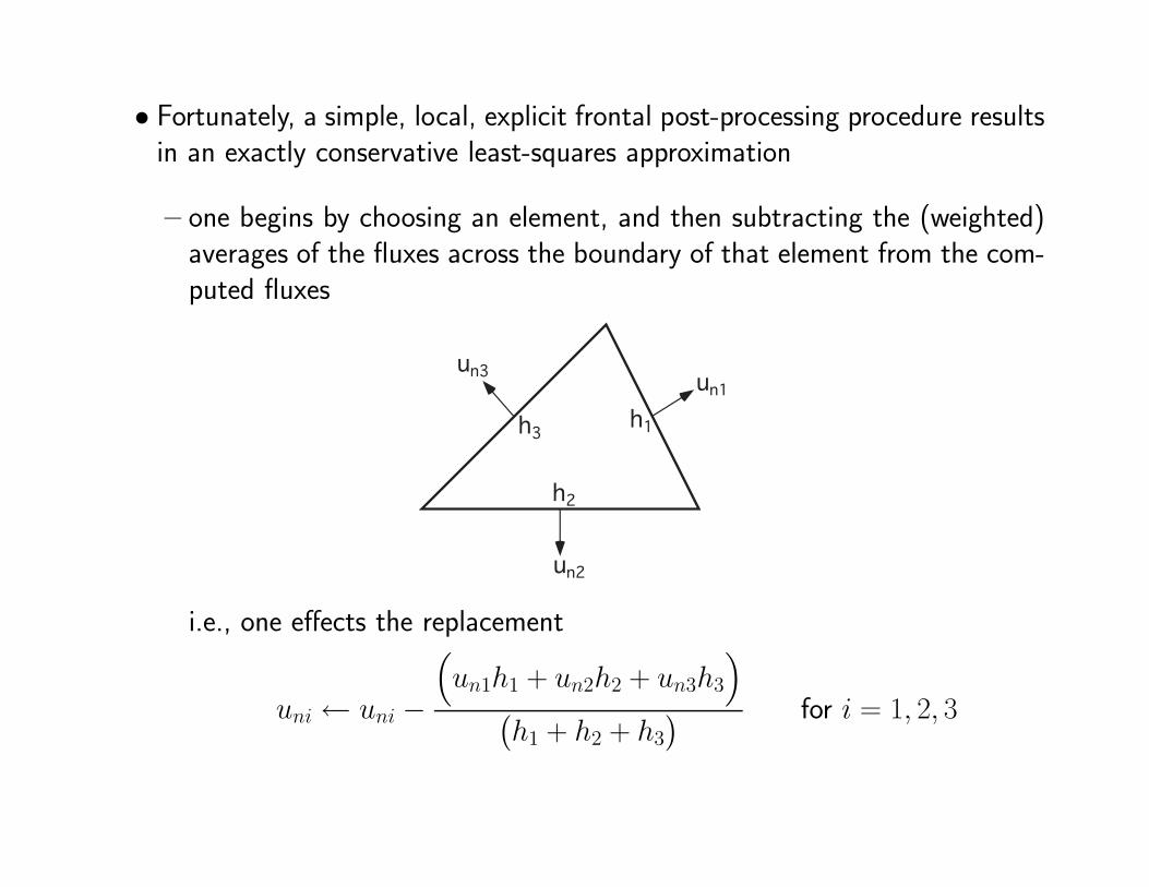
• Fortunately, a simple, local, explicit frontal post-processing procedure resultsin an exactly conservative least-squares approximation

– one begins by choosing an element, and then subtracting the (weighted)averages of the fluxes across the boundary of that element from the com-puted fluxes

un2

h2

un1

h1

un3

h3

i.e., one effects the replacement

uni← uni −

(un1h1 + un2h2 + un3h3

)

(h1 + h2 + h3

) for i = 1, 2, 3

– one then repeats this process in all the triangles, one at a time, exceptthat if a flux has been previously been updated, then it is left unchanged

e.g., if un1 has already been updated, we have that

un1← un1

and

uni ← uni −

(un1h1 + un2h2 + un3h3

)

(h2 + h3

) for i = 2, 3

• The post-processing procedure results in a new flux approximation uh for

which

un1h1 + un2h2 + un3h3 = 0

in every triangle

• The accuracy of uh itself and of φh is not affected

0 5 10 15 20 250

5

10

15

20

25

-4·10-7 -2·10-7 0 2·10-7 4·10-70

20

40

60

80

0 5 10 15 20 250

5

10

15

20

25

0 5·10-16 1·10-15 1.5·10-15 2·10-150

100

200

300

400

500

600

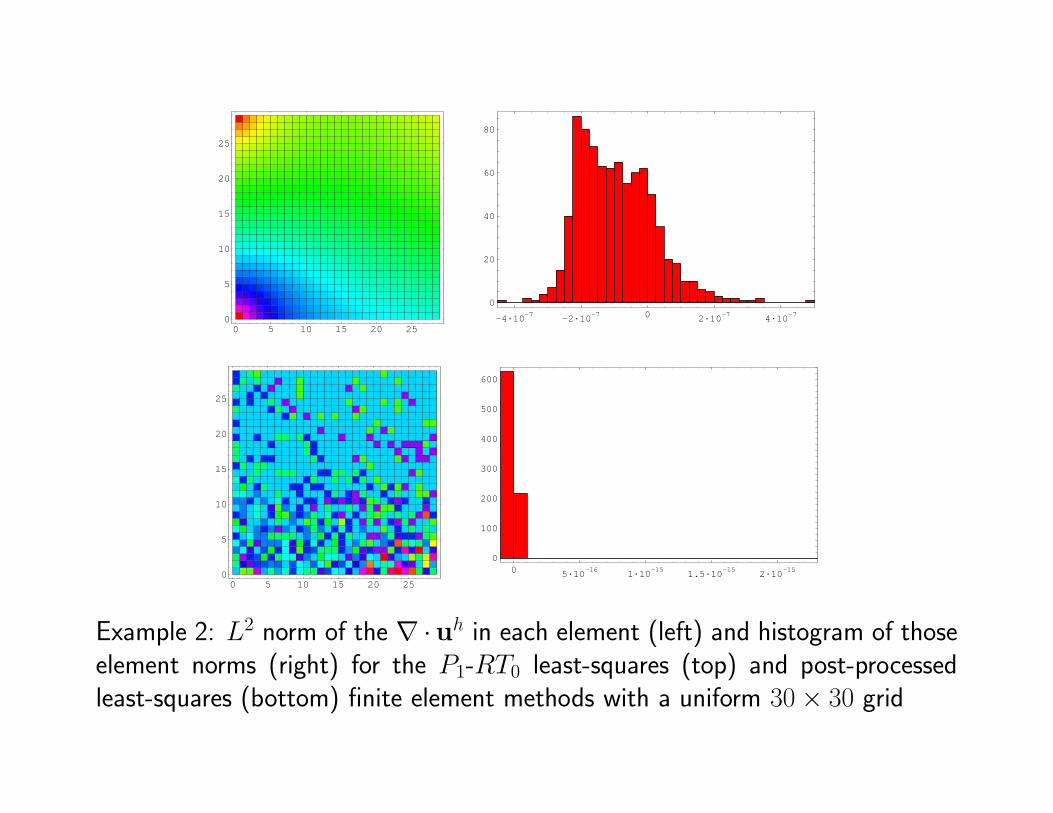
Example 2: L2 norm of the ∇ ·uh in each element (left) and histogram of thoseelement norms (right) for the P1-RT0 least-squares (top) and post-processedleast-squares (bottom) finite element methods with a uniform 30× 30 grid

0 5 10 15 20 250

5

10

15

20

25

0 5·10-16 1·10-15 1.5·10-15 2·10-15 2.5·10-150

100

200

300

400

500

600

0 5 10 15 20 250

5

10

15

20

25

0 5·10-16 1·10-15 1.5·10-15 2·10-150

100

200

300

400

500

600

Example 2: L2 norm of the ∇ ·uh in each element (left) and histogram of thoseelement norms (right) for the P0-RT0 mixed-Galerkin (top) and the P1-RT0

post-processed least-squares (bottom) finite element methods

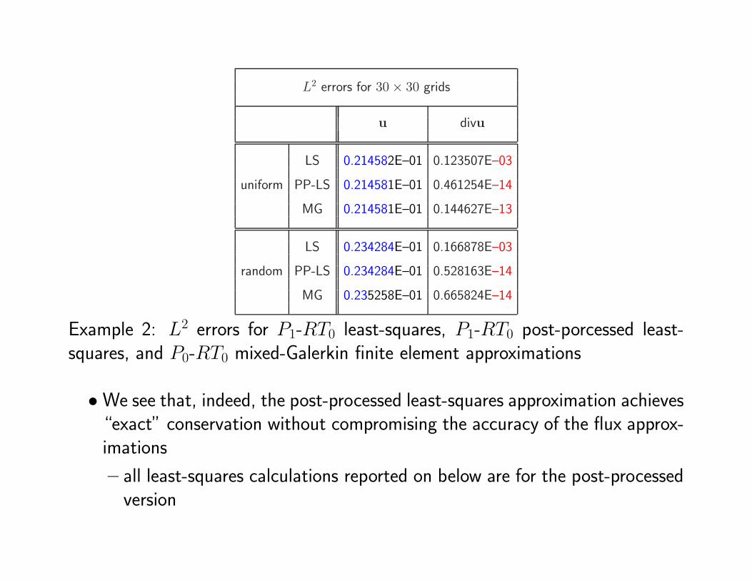
L2 errors for 30× 30 grids

u divu

LS 0.214582E–01 0.123507E–03

uniform PP-LS 0.214581E–01 0.461254E–14

MG 0.214581E–01 0.144627E–13

LS 0.234284E–01 0.166878E–03

random PP-LS 0.234284E–01 0.528163E–14

MG 0.235258E–01 0.665824E–14

Example 2: L2 errors for P1-RT0 least-squares, P1-RT0 post-porcessed least-squares, and P0-RT0 mixed-Galerkin finite element approximations

•We see that, indeed, the post-processed least-squares approximation achieves“exact” conservation without compromising the accuracy of the flux approx-imations

– all least-squares calculations reported on below are for the post-processedversion

L2 errors vs. number of grid points for uniform grids

4 8 16 32 64 128

u LS 2.07322E–01 8.88903E–02 4.14851E–02 2.00738E–02 9.87759E–03 4.89991E–04

MG 2.07305E–01 8.88966E–02 4.14847E–02 2.00737E–02 9.87758E–03 4.89991E–04

divu LS 5.64894E–16 1.10648E–15 2.49139E–15 5.18163E–15 1.03237E–14 2.12458E–14

MG 3.16192E–16 2.01247E–15 4.66477E–15 2/73818E–14 1.81733E–14 4.38308E–14

φ LS 9.20114E–03 1.66275E–03 3.60709E–04 8.43673E–05 2.04219E–05 5.02501E–06

MG 1.71312E–01 7.36546E–02 3.43916E–02 1.66431E–02 8.18971E–03 4.06264E–03

Example 2: L2 errors vs. number of grid points in each direction for P1-RT0

least-squares and P0-RT0 mixed-Galerkin finite element approximations

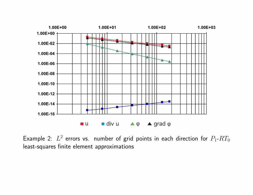
u div u φ grad φ

Example 2: L2 errors vs. number of grid points in each direction for P1-RT0

least-squares finite element approximations

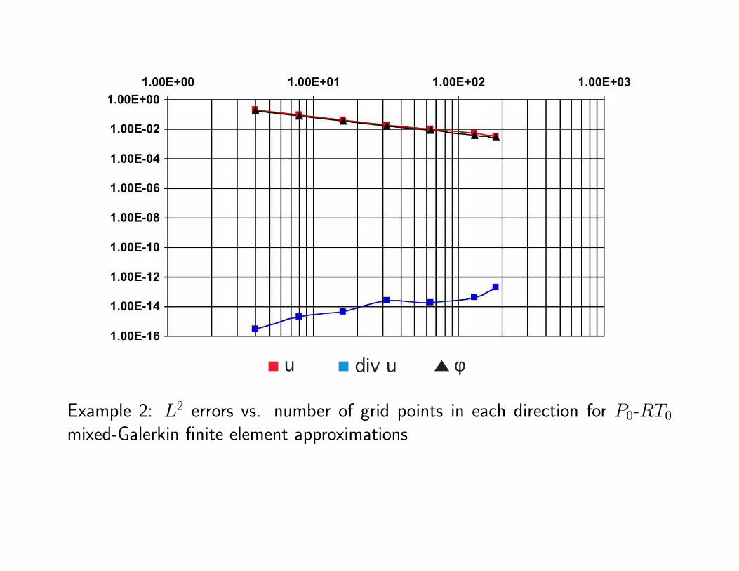
u div u φ

Example 2: L2 errors vs. number of grid points in each direction for P0-RT0

mixed-Galerkin finite element approximations

L2 errors for a 25× 25

randomly perturbed

nonuniform grid

LS MG

u 0.356537E–01 0.356303E–01

divu 0.34923E–14 0.45140E–14

φ 0.316519E–03 0.110673E+00

gradφ 0.239616E–01 N/A

Example 2: L2 errors for P1-RT0 least-squares and P0-RT0 mixed-Galerkin finiteelement approximations

5 10 15 20 25

5

10

15

20

25

5 10 15 20 25

5

10

15

20

25

5 10 15 20 25

5

10

15

20

25

510

1520

25510152025

00.511.52

510

1520

25

510

1520

25510152025

11.52

2.5

510

1520

25

5101520

25510152025

-2-1.5-1-0.50

5101520

25

Example 2: P1-RT0 least-squares finite element approximation on a 25 × 25randomly perturbed nonuniform grid

left: x-component of u

center: y-component of u

right: φ

5 10 15 20 25

5

10

15

20

25

5 10 15 20 25

5

10

15

20

25

5 10 15 20 25

5

10

15

20

25

510

1520

25510152025

00.511.52

510

1520

25

510

1520

25510152025

11.52

2.5

510

1520

25

510

1520

25510152025

-2-10

510

1520

25

Example 2: P0-RT0 mixed-Galerkin finite element approximation on a 25 × 25randomly perturbed nonuniform grid

left: x-component of u

center: y-component of u

right: φ

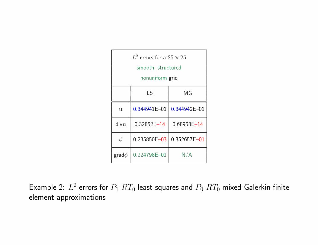
L2 errors for a 25× 25

smooth, structured

nonuniform grid

LS MG

u 0.344941E–01 0.344942E–01

divu 0.32852E–14 0.68958E–14

φ 0.235850E–03 0.352657E–01

gradφ 0.224798E–01 N/A

Example 2: L2 errors for P1-RT0 least-squares and P0-RT0 mixed-Galerkin finiteelement approximations

5 10 15 20 25

5

10

15

20

25

5 10 15 20 25

5

10

15

20

25

5 10 15 20 25

5

10

15

20

25

510

1520

25510152025

00.511.52

510

1520

25

510

1520

25510152025

11.52

2.5

510

1520

25

5101520

25510152025

-2-1.5-1-0.50

5101520

25

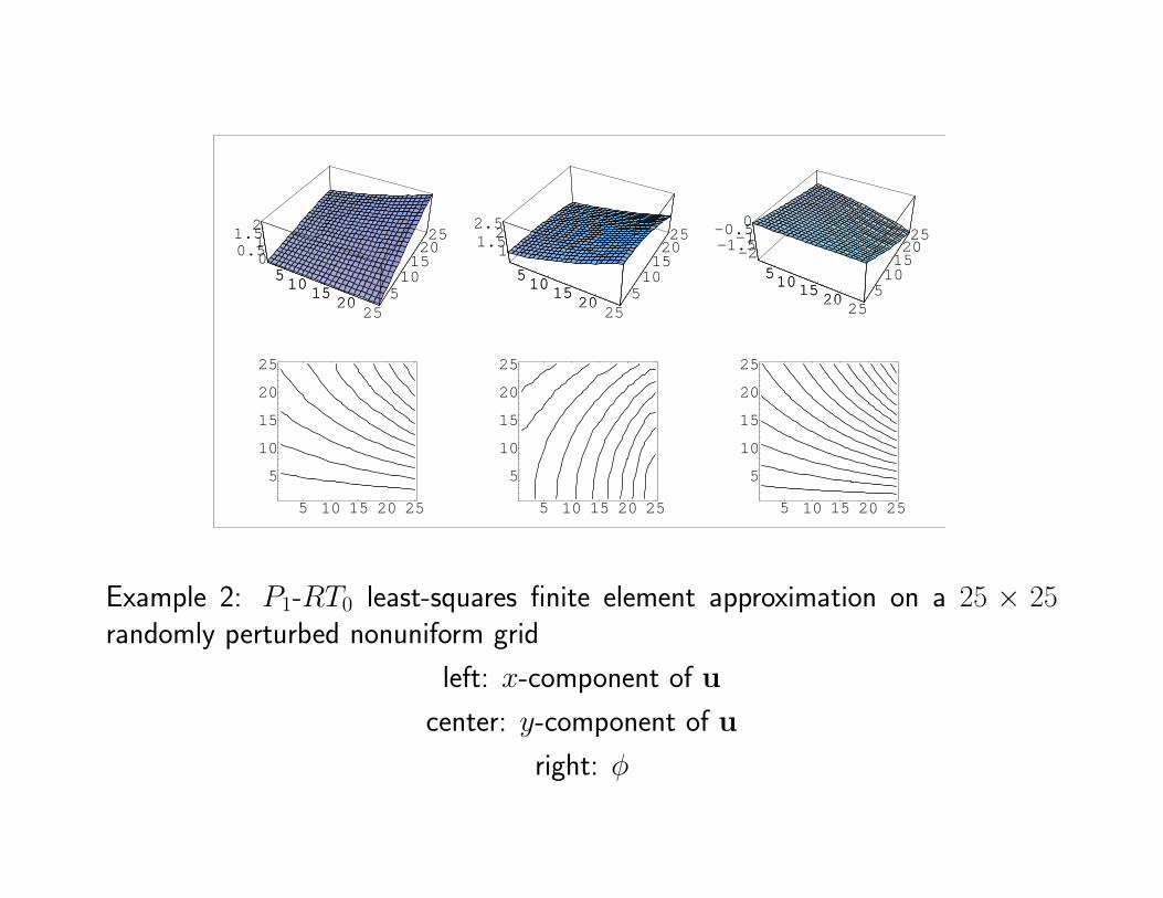
Example 2: P1-RT0 least-squares finite element approximation on a 25 × 25smooth, structured nonuniform grid

left: x-component of u

center: y-component of u

right: φ

5 10 15 20 25

5

10

15

20

25

5 10 15 20 25

5

10

15

20

25

5 10 15 20 25

5

10

15

20

25

510

1520

25510152025

00.511.52

510

1520

25

510

1520

25510152025

11.52

2.5

510

1520

25

5101520

25510152025

-2-1.5-1-0.5

0

5101520

25

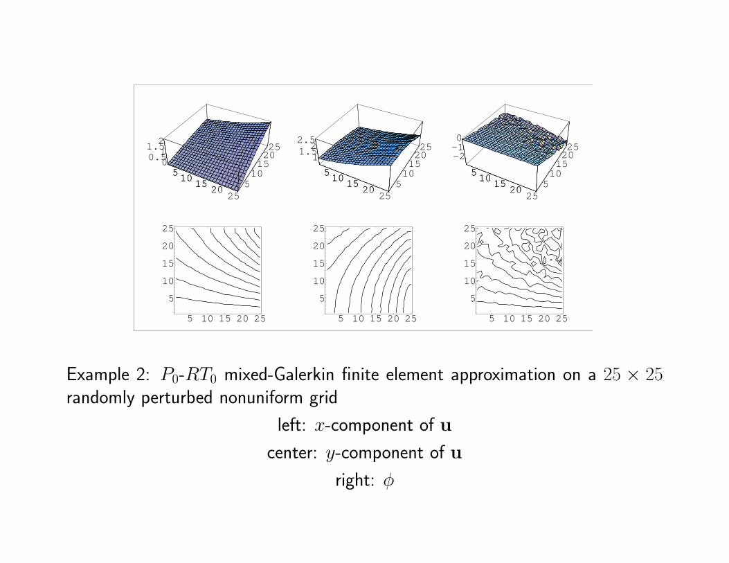
Example 2: P0-RT0 mixed-Galerkin finite element approximation on a 25 × 25smooth, structured nonuniform grid

left: x-component of u

center: y-component of u

right: φ

5 10 15 20 25

5

10

15

20

25

510

1520

25

5

10

15

2025

-2-1.5-1

-0.50

510

1520

25

5 10 15 20 25

5

10

15

20

25

510

1520

25

5

10

15

20

25

-2

-1

0

510

1520

25

Example 2: P1-RT0 least-squares (top) and P0-RT0 mixed-Galerkin (bottom)finite element approximations of φ on a 25× 25 randomly perturbed nonuniformgrid

5 10 15 20 25

5

10

15

20

25

510

1520

25

5

10

15

2025

-2-1.5-1

-0.50

510

1520

25

5 10 15 20 25

5

10

15

20

25

510

1520

25

5

10

15

2025

-2-1.5-1

-0.50

510

1520

25

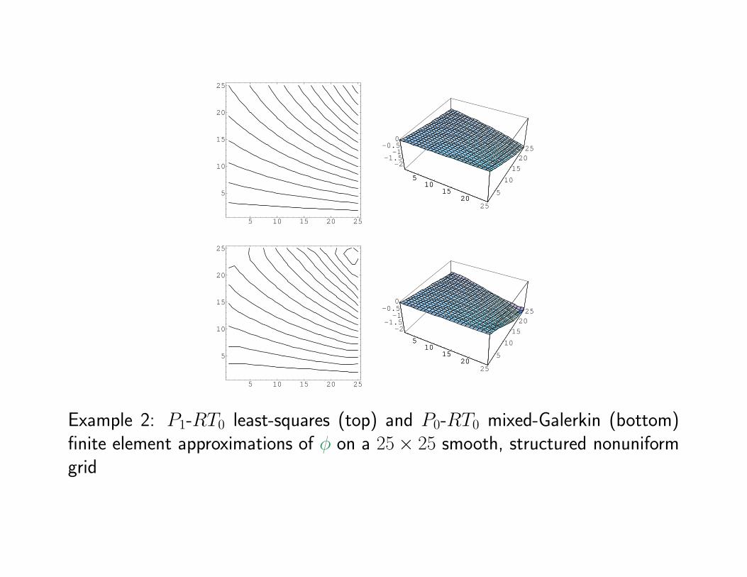
Example 2: P1-RT0 least-squares (top) and P0-RT0 mixed-Galerkin (bottom)finite element approximations of φ on a 25× 25 smooth, structured nonuniformgrid