Lattice Quantum Chromodynamics - Τομέας Φυσικήςphysik_uni-wuppertal... · Lattice...

Lattice Quantum Chromodynamics

Francesco Knechtli

Bergische Universitat Wuppertal

8th September, 2016

Summer School on the Standard Model and Beyond, Corfu

Outline Lattice QCD Continuum limit Monte Carlo simulations Static quark potential Some results Conclusions

Outline

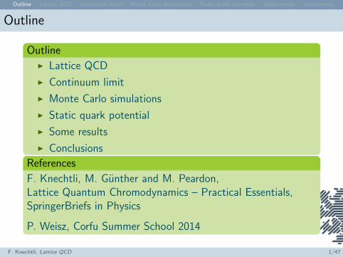
OutlineI Lattice QCD

I Continuum limit

I Monte Carlo simulations

I Static quark potential

I Some results

I Conclusions

References

F. Knechtli, M. Gunther and M. Peardon,Lattice Quantum Chromodynamics – Practical Essentials,SpringerBriefs in Physics

P. Weisz, Corfu Summer School 2014

F. Knechtli, Lattice QCD 1/47


Lattice QCD



Quantumchromodynamics (QCD)

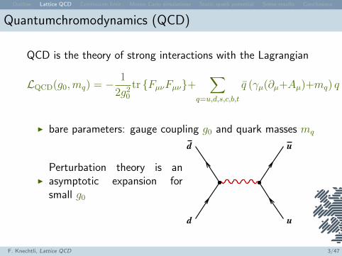
QCD is the theory of strong interactions with the Lagrangian

LQCD(g0,mq) = − 1

2g20

tr FµνFµν+∑

q=u,d,s,c,b,t

q (γµ(∂µ+Aµ)+mq) q

I bare parameters: gauge coupling g0 and quark masses mq

I

Perturbation theory is anasymptotic expansion forsmall g0

u

ud

d



Asymptotic freedom

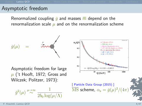
Renormalized coupling g and masses m depend on therenormalization scale µ and on the renormalization scheme

g(µ) =µ

Asymptotic freedom for largeµ (’t Hooft, 1972; Gross andWilczek; Politzer, 1973):

g2(µ)µ→∞∼ 1

2b0 log(µ/Λ)

QCD αs(Mz) = 0.1181 ± 0.0013

pp –> jetse.w. precision fits (NNLO)

0.1

0.2

0.3

αs (Q2)

1 10 100Q [GeV]

Heavy Quarkonia (NLO)

e+e– jets & shapes (res. NNLO)

DIS jets (NLO)

October 2015

τ decays (N3LO)

1000

(NLO

pp –> tt (NNLO)

)(–)

[ Particle Data Group (2015) ]

MS scheme, αs = g(µ)2/(4π)



Confinement

Regimes of QCD

I Perturbation theory works at high energy & 2 GeV whereαs is small and quarks and gluons are (almost) free

I At lower energies, quarks and gluons are confined intohadrons ⇒ we need a different tool to extract from LQCD

the properties of hadrons: lattice formulation andcomputer simulations



Gauge theory on the lattice

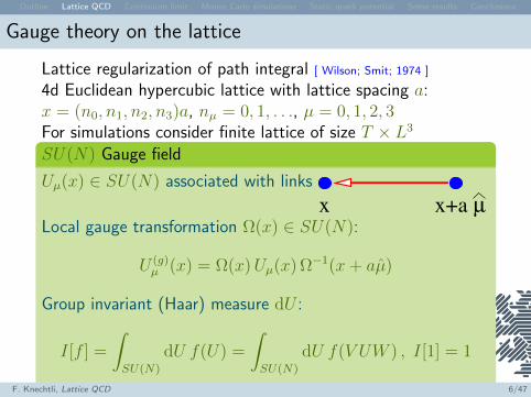
Lattice regularization of path integral [ Wilson; Smit; 1974 ]

4d Euclidean hypercubic lattice with lattice spacing a:x = (n0, n1, n2, n3)a, nµ = 0, 1, . . ., µ = 0, 1, 2, 3For simulations consider finite lattice of size T × L3

SU(N) Gauge field

Uµ(x) ∈ SU(N) associated with links

x x+a µ

Local gauge transformation Ω(x) ∈ SU(N):

U (g)µ (x) = Ω(x)Uµ(x) Ω−1(x+ aµ)

Group invariant (Haar) measure dU :

I[f ] =

∫SU(N)

dU f(U) =

∫SU(N)

dU f(V UW ) , I[1] = 1



Wilson gauge action

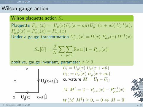
Wilson plaquette action Sw

Plaquette Pµ,ν(x) = Uµ(x)Uν(x + aµ)U−1µ (x + aν)U−1

ν (x),P−1µ,ν(x) = P †µ,ν(x) = Pν,µ(x)

Under a gauge transformation U ′µ,ν(x) = Ω(x) Pµ,ν(x) Ω−1(x)

Sw[U ] =β

N

∑x

∑µ<ν

Re tr [1− Pµ,ν(x)]

positive, gauge invariant, parameter β ≥ 0

x x+a µU (x)µ

νµU (x+a )

UI = Uµ(x) Uν(x+ aµ)UII = Uν(x) Uµ(x+ aν)curvature M = UI − UII

M M † = 2− Pµ,ν(x)− P−1µ,ν(x)

tr (M M †) ≥ 0, = 0 ⇔ M = 0F. Knechtli, Lattice QCD 7/47


Lattice path integral

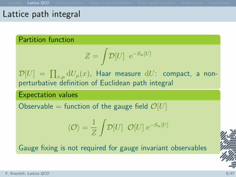
Partition function

Z =

∫D[U ] e−Sw[U ]

D[U ] =∏

x,µ dUµ(x), Haar measure dU : compact, a non-perturbative definition of Euclidean path integral

Expectation values

Observable = function of the gauge field O[U ]

〈O〉 =1

Z

∫D[U ] O[U ] e−Sw[U ]

Gauge fixing is not required for gauge invariant observables



Wilson fermions

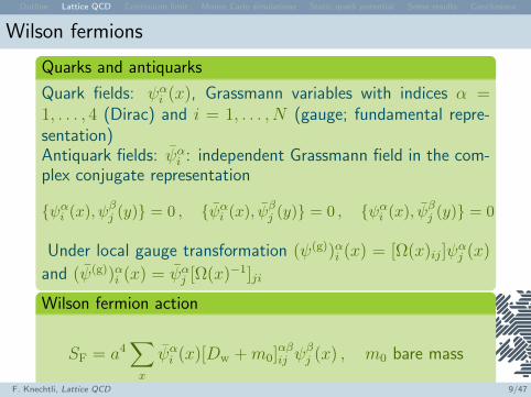
Quarks and antiquarks

Quark fields: ψαi (x), Grassmann variables with indices α =1, . . . , 4 (Dirac) and i = 1, . . . , N (gauge; fundamental repre-sentation)Antiquark fields: ψαi : independent Grassmann field in the com-plex conjugate representation

ψαi (x), ψβj (y) = 0 , ψαi (x), ψβj (y) = 0 , ψαi (x), ψβj (y) = 0

Under local gauge transformation (ψ(g))αi (x) = [Ω(x)ij]ψαj (x)

and (ψ(g))αi (x) = ψαj [Ω(x)−1]ji

Wilson fermion action

SF = a4∑x

ψαi (x)[Dw +m0]αβij ψβj (x) , m0 bare mass



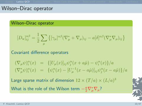
Wilson–Dirac operator


[Dw]αβij =1

2

∑µ

[γµ]αβ(∇∗µ +∇µ)ij − a[δ]αβ(∇∗µ∇µ)ij

Covariant difference operators

(∇µψ)αi (x) = [Uµ(x)]ijψαj (x+ aµ)− ψαi (x)/a

(∇∗µψ)αi (x) = ψαi (x)− [U−1µ (x− aµ)]ijψ

αj (x− aµ)/a

Large sparse matrix of dimension 12× (T/a)× (L/a)3

What is the role of the Wilson term −a2∇∗µ∇µ?



Chiral symmetry

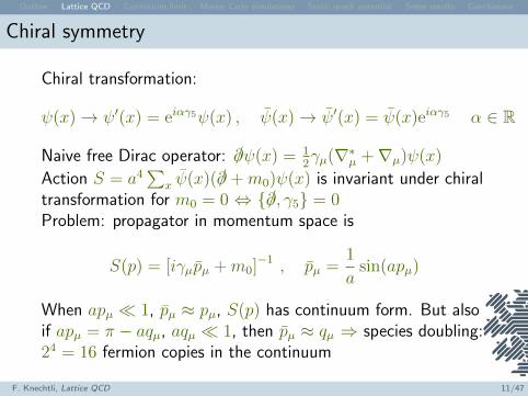
Chiral transformation:

ψ(x)→ ψ′(x) = eiαγ5ψ(x) , ψ(x)→ ψ′(x) = ψ(x)eiαγ5 α ∈ R

Naive free Dirac operator: /∂ψ(x) = 12γµ(∇∗µ +∇µ)ψ(x)

Action S = a4∑

x ψ(x)(/∂ +m0)ψ(x) is invariant under chiraltransformation for m0 = 0 ⇔ /∂, γ5 = 0Problem: propagator in momentum space is

S(p) = [iγµpµ +m0]−1 , pµ =1

asin(apµ)

When apµ 1, pµ ≈ pµ, S(p) has continuum form. But alsoif apµ = π − aqµ, aqµ 1, then pµ ≈ qµ ⇒ species doubling:24 = 16 fermion copies in the continuum



Nielsen–Ninomiya theorem

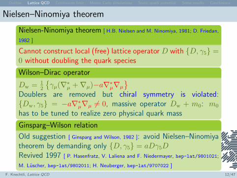
Nielsen-Ninomiya theorem [ H.B. Nielsen and M. Ninomiya, 1981; D. Friedan,

1982 ]

Cannot construct local (free) lattice operator D with D, γ5 =0 without doubling the quark species


Dw = 12

γµ(∇∗µ +∇µ)−a∇∗µ∇µ

Doublers are removed but chiral symmetry is violated:Dw, γ5 = −a∇∗µ∇µ 6= 0, massive operator Dw + m0: m0

has to be tuned to realize zero physical quark mass

Ginsparg–Wilson relation

Old suggestion [ Ginsparg and Wilson, 1982 ]: avoid Nielsen–Ninomiyatheorem by demanding only D, γ5 = aDγ5DRevived 1997 [ P. Hasenfratz, V. Laliena and F. Niedermayer, hep-lat/9801021;

M. Luscher, hep-lat/9802011; H. Neuberger, hep-lat/9707022 ]



Lattice QCD

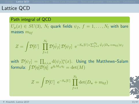
Path integral of QCD

Uµ(x) ∈ SU(3), Nf quark fields ψf , f = 1, . . . , Nf with baremasses m0f

Z =

∫D[U ]

Nf∏f=1

D[ψf ]D[ψf ] e−Sw[U ]+∑Nff=1 ψf (Dw+m0f )ψf

with D[ψf ] =∏

x,i,α d(ψf )αi (x). Using the Matthews–Salam

formula:∫D[η]D[η] eηiMijηj = det(M)

Z =

∫D[U ] e−Sw[U ]

Nf∏f=1

det(Dw +m0f )



Nucleon

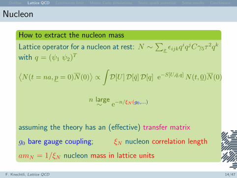
How to extract the nucleon mass

Lattice operator for a nucleon at rest: N ∼∑x εijkqiqjCγ5τ

2qk

with q = (ψ1 ψ2)T

⟨N(t = na, p = 0)N(0)

⟩∝∫D[U ]D[q]D[q] e−S[U,q,q]N(t, 0)N(0)

n large∼ e−n/ξN (g0,...)

assuming the theory has an (effective) transfer matrix

g0 bare gauge coupling; ξN nucleon correlation length

amN = 1/ξN nucleon mass in lattice units



Continuum limit



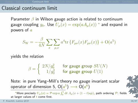
Classical continuum limit

Parameter β in Wilson gauge action is related to continuumgauge coupling g0. Use Uµ(x) = exp(aAµ(x)) ∗ and expand inpowers of a

SW = − β

4N

∑x

∑µ,ν

a4tr Fµν(x)Fµν(x)+ O(a5)

yields the relation

β =

2N/g2

0 for gauge group SU(N)1/g2

0 for gauge group U(1)

Note: in pure Yang–Mill’s theory no gauge invariant scalaroperator of dimension 5, O(a5) −→ O(a6)∗More precisely Uµ(x) = P exp a

∫ 10 dt Aµ(x+ (1− t)aµ), path ordering P: fields

at larger values of t come first.



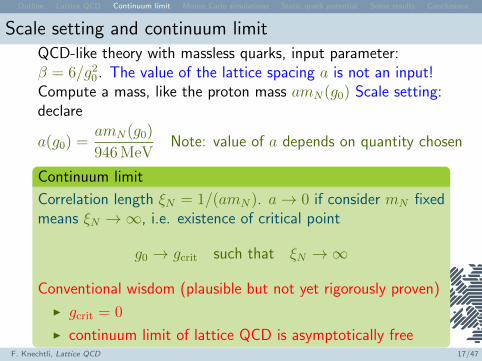
Scale setting and continuum limitQCD-like theory with massless quarks, input parameter:β = 6/g2

0. The value of the lattice spacing a is not an input!Compute a mass, like the proton mass amN(g0) Scale setting:declare

a(g0) =amN(g0)

946 MeVNote: value of a depends on quantity chosen

Continuum limit

Correlation length ξN = 1/(amN). a→ 0 if consider mN fixedmeans ξN →∞, i.e. existence of critical point

g0 → gcrit such that ξN →∞

Conventional wisdom (plausible but not yet rigorously proven)

I gcrit = 0

I continuum limit of lattice QCD is asymptotically freeF. Knechtli, Lattice QCD 17/47


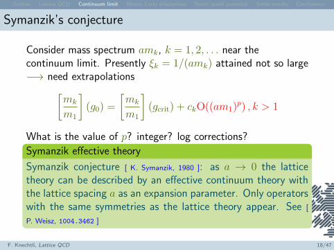
Symanzik’s conjecture

Consider mass spectrum amk, k = 1, 2, . . . near thecontinuum limit. Presently ξk = 1/(amk) attained not so large−→ need extrapolations[

mk

m1

](g0) =

[mk

m1

](gcrit) + ckO((am1)p) , k > 1

What is the value of p? integer? log corrections?

Symanzik effective theory

Symanzik conjecture [ K. Symanzik, 1980 ]: as a → 0 the latticetheory can be described by an effective continuum theory withthe lattice spacing a as an expansion parameter. Only operatorswith the same symmetries as the lattice theory appear. See [

P. Weisz, 1004.3462 ]



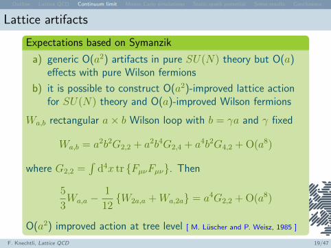
Lattice artifacts

Expectations based on Symanzik

a) generic O(a2) artifacts in pure SU(N) theory but O(a)effects with pure Wilson fermions

b) it is possible to construct O(a2)-improved lattice actionfor SU(N) theory and O(a)-improved Wilson fermions

Wa,b rectangular a× b Wilson loop with b = γa and γ fixed

Wa,b = a2b2G2,2 + a2b4G2,4 + a4b2G4,2 + O(a8)

where G2,2 =∫

d4x tr FµνFµν. Then

5

3Wa,a −

1

12W2a,a +Wa,2a = a4G2,2 + O(a8)

O(a2) improved action at tree level [ M. Luscher and P. Weisz, 1985 ]



Monte Carlo simulations



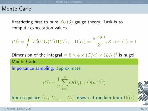
Monte Carlo

Restricting first to pure SU(3) gauge theory. Task is tocompute expectation values

〈O〉 =

∫D[U ]O(U) Π(U) , Π(U) =

e−S(U)

Z,Z ↔ 〈1〉 = 1

Dimension of the integral = 8× 4× (T/a)× (L/a)3 is huge!

Monte Carlo

Importance sampling: approximate

〈O〉 =1

n

n∑i=1

O(Ui) + O(n−1/2)

from sequence U1, U2, . . . , Un drawn at random from Π(U)



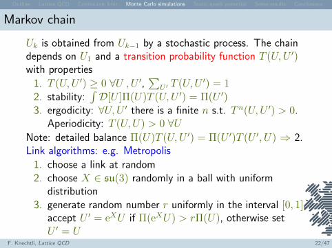
Markov chain

Uk is obtained from Uk−1 by a stochastic process. The chaindepends on U1 and a transition probability function T (U,U ′)with properties

1. T (U,U ′) ≥ 0 ∀U ,U ′, ∑U ′ T (U,U ′) = 12. stability:

∫D[U ]Π(U)T (U,U ′) = Π(U ′)

3. ergodicity: ∀U,U ′ there is a finite n s.t. T n(U,U ′) > 0.Aperiodicity: T (U,U) > 0 ∀U

Note: detailed balance Π(U)T (U,U ′) = Π(U ′)T (U ′, U) ⇒ 2.Link algorithms: e.g. Metropolis

1. choose a link at random2. choose X ∈ su(3) randomly in a ball with uniform

distribution3. generate random number r uniformly in the interval [0, 1],

accept U ′ = eXU if Π(eXU) > rΠ(U), otherwise setU ′ = U



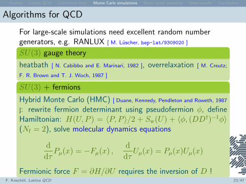
Algorithms for QCD

For large-scale simulations need excellent random numbergenerators, e.g. RANLUX [ M. Luscher, hep-lat/9309020 ]

SU(3) gauge theory

heatbath [ N. Cabibbo and E. Marinari, 1982 ], overrelaxation [ M. Creutz;

F. R. Brown and T. J. Woch, 1987 ]

SU(3) + fermions

Hybrid Monte Carlo (HMC) [ Duane, Kennedy, Pendleton and Roweth, 1987

]: rewrite fermion determinant using pseudofermion φ, defineHamiltonian: H(U, P ) = 〈P, P 〉/2 + Sw(U) + 〈φ, (DD†)−1φ〉(Nf = 2), solve molecular dynamics equations

d

dτPµ(x) = −Fµ(x) ,

d

dτUµ(x) = Pµ(x)Uµ(x)

Fermionic force F = ∂H/∂U requires the inversion of D !F. Knechtli, Lattice QCD 23/47


Statistical error analysis

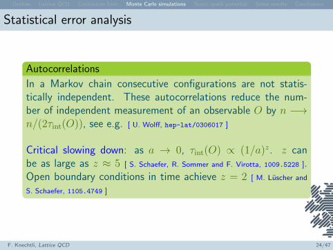
Autocorrelations

In a Markov chain consecutive configurations are not statis-tically independent. These autocorrelations reduce the num-ber of independent measurement of an observable O by n −→n/(2τint(O)), see e.g. [ U. Wolff, hep-lat/0306017 ]

Critical slowing down: as a → 0, τint(O) ∝ (1/a)z. z canbe as large as z ≈ 5 [ S. Schaefer, R. Sommer and F. Virotta, 1009.5228 ].Open boundary conditions in time achieve z = 2 [ M. Luscher and

S. Schaefer, 1105.4749 ]



Static quark potential



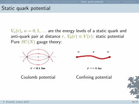
Static quark potential

Vn(r), n = 0, 1, . . . are the energy levels of a static quark andanti-quark pair at distance r. V0(r) ≡ V (r): static potentialPure SU(N) gauge theory:

Coulomb potential Confining potential



Short distance

Small distance

SU(N) + fermions: as r → 0 perturbation theory can be ap-plied (asymptotic freedom)

V (r)r→0∼ −CF

g20

4πr, CF = (N2 − 1)/(2N)

Expansion of V (r) in the MS coupling is known to 3 loops[ N. Brambilla, A. Pineda, J. Soto, A. Vairo, hep-ph/9907240, hep-ph/9903355;

A. V. Smirnov, V. A. Smirnov and M. Steinhauser, 0911.4742; C. Anzai, Y. Kiyo

and Y. Sumino, 0911.4335 ]



Bosonic string

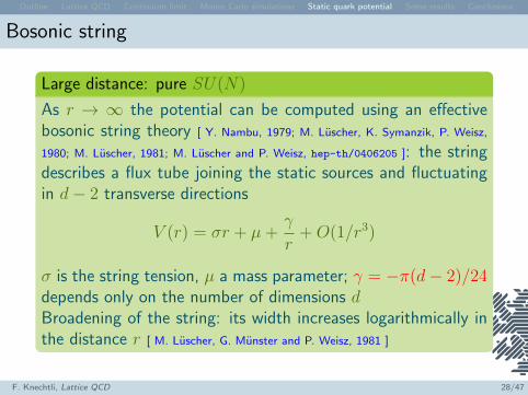
Large distance: pure SU(N)

As r → ∞ the potential can be computed using an effectivebosonic string theory [ Y. Nambu, 1979; M. Luscher, K. Symanzik, P. Weisz,

1980; M. Luscher, 1981; M. Luscher and P. Weisz, hep-th/0406205 ]: the stringdescribes a flux tube joining the static sources and fluctuatingin d− 2 transverse directions

V (r) = σr + µ+γ

r+O(1/r3)

σ is the string tension, µ a mass parameter; γ = −π(d− 2)/24depends only on the number of dimensions dBroadening of the string: its width increases logarithmically inthe distance r [ M. Luscher, G. Munster and P. Weisz, 1981 ]



String breaking

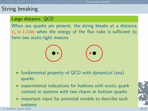
Large distance: QCD

When sea quarks are present, the string breaks at a distancerb ≈ 1.5 fm when the energy of the flux tube is sufficient toform two static-light mesons

I fundamental property of QCD with dynamical (sea)quarks

I experimental indications for hadrons with exotic quarkcontent in systems with two charm or bottom quarks

I important input for potential models to describe suchsystems



Static force and strong coupling

Static force F

The potential contains an additive constant which divergeswhen the ultra-violet cut-off (1/a) goes to infinity. The di-vergence originates from the self-energy of the static quarks.A renormalized quantity is the static force F (r) = dV (r)/dr

Runnning coupling

αqq(µ) ≡ g2qq(µ)

4π=

1

CF

r2F (r)

coupling gqq(µ) runs with the energy scale µ = 1/r

µd

dµgqq(µ) = βqq(gqq(µ))

βqq function is known up to the 4-loop term, cf. [ M. Donnellan,

F. Knechtli, B. Leder and R. Sommer, 1012.3037 ]F. Knechtli, Lattice QCD 30/47


Renormalization group equation

µd

dµgqq(µ) = βqq(gqq(µ))

βqq(gqq) = −g3qq[

3∑n=0

b(qq)n g2n

qq + b(qq)3,l g

6qq log(3g2

qq/(8π)) + O(g8qq)]

b(qq)0 = b0 = 1

(4π)2

(11− 2

3Nf

), b

(qq)1 = b1 = 1

(4π)4

(102− 38

3 Nf

)Integration of renormalization group equation

Λqq = µ(b0g

2qq

)−b1/(2b20)e−1/(2b0g2qq)

× exp

−∫ gqq

0

dx

[1

β(x)+

1

b0x3− b1

b20x

]Λqq is the Λ parameter in the qq scheme

n-loop solution: truncate βqq after term b(qq)n−1 and solve for gqq



Static force and scale r0

Setting the scale from the static force

r2F (r)|r=r(c) = c

c = 1.65 leads to the scale r0 = r(1.65) which has a value ofabout 0.5 fm in QCD [ R. Sommer, hep-lat/9310022 ]

Other choices are r1 = r(1.0) [ C. W. Bernard, T. Burch, K. Orginos,

D. Toussaint, T. A. DeGrand, C. E. DeTar, S. A. Gottlieb, U. M. Heller, J. E. Hetrick

and B. Sugar, hep-lat/0002028 ] and rc = r(0.65) [ S. Necco and R. Sommer,

hep-lat/0108008 ]



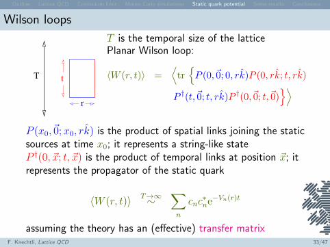
Wilson loops

T t

r

T is the temporal size of the latticePlanar Wilson loop:

〈W (r, t)〉 =⟨

trP (0,~0; 0, rk)P (0, rk; t, rk)

P †(t,~0; t, rk)P †(0,~0; t,~0)⟩

P (x0,~0;x0, rk) is the product of spatial links joining the staticsources at time x0; it represents a string-like stateP †(0, ~x; t, ~x) is the product of temporal links at position ~x; itrepresents the propagator of the static quark

〈W (r, t)〉 T→∞∼∑n

cnc∗ne−Vn(r)t

assuming the theory has an (effective) transfer matrixF. Knechtli, Lattice QCD 33/47


Generalized eigenvalue problem

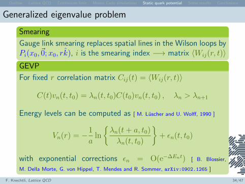
Smearing

Gauge link smearing replaces spatial lines in the Wilson loops byPi(x0,~0;x0, rk), i is the smearing index −→ matrix 〈Wij(r, t)〉GEVP

For fixed r correlation matrix Cij(t) = 〈Wij(r, t)〉

C(t)vn(t, t0) = λn(t, t0)C(t0)vn(t, t0) , λn > λn+1

Energy levels can be computed as [ M. Luscher and U. Wolff, 1990 ]

Vn(r) = −1

aln

λn(t+ a, t0)

λn(t, t0)

+ εn(t, t0)

with exponential corrections εn = O(e−∆Ent) [ B. Blossier,

M. Della Morte, G. von Hippel, T. Mendes and R. Sommer, arXiv:0902.1265 ]



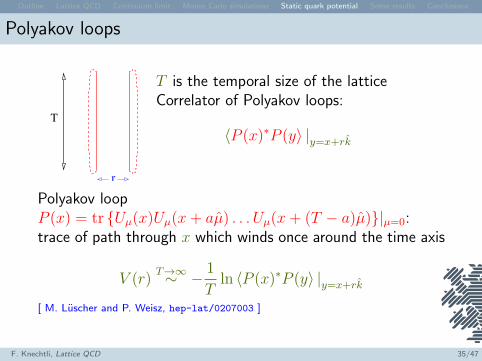
Polyakov loops

T

r

T is the temporal size of the latticeCorrelator of Polyakov loops:

〈P (x)∗P (y〉 |y=x+rk

Polyakov loopP (x) = tr Uµ(x)Uµ(x+ aµ) . . . Uµ(x+ (T − a)µ)|µ=0:trace of path through x which winds once around the time axis

V (r)T→∞∼ − 1

Tln 〈P (x)∗P (y〉 |y=x+rk

[ M. Luscher and P. Weisz, hep-lat/0207003 ]



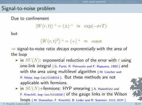
Signal-to-noise problem

Due to confinement

〈W (r, t)〉 “ = 〈±〉 “ ≈ exp(−σrT )

but ⟨W (r, t)2

⟩“ = 〈+〉 “ ≈ const

⇒ signal-to-noise ratio decays exponentially with the area ofthe loop

I in SU(N): exponential reduction of the error with t usingone-link integral [ G. Parisi, R. Petronzio and F. Rapuano, 1983 ] andwith the area using multilevel algorithm [ M. Luscher and

P. Weisz, hep-lat/0108014 ]. But these methods are notapplicable with fermions.

I in SU(N)+fermions: HYP smearing [ A. Hasenfratz and

F. Knechtli, hep-lat/0103029 ] of the gauge links in the Wilsonloops [ M. Donnellan, F. Knechtli, B. Leder and R. Sommer, 1012.3037 ]



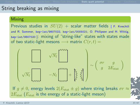
String breaking as mixing

Mixing

Previous studies in SU(2) + scalar matter fields [ F. Knechtli

and R. Sommer, hep-lat/9807022, hep-lat/0005021; O. Philipsen and H. Wittig,

hep-lat/9807020 ]: mixing of “string-like” states with states madeof two static-light mesons −→ matrix C(r, t) =

√Nf

√Nf −Nf +

∼(σr gg 2Estat

)

If g 6= 0, energy levels 2(Estat ± g) where string breaks σr ≈2Estat (Estat is the energy of a static-light meson)



Some results



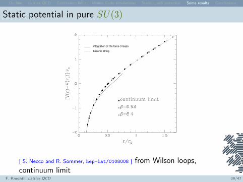
Static potential in pure SU(3)

integration of the force-3 loops

bosonic string

[ S. Necco and R. Sommer, hep-lat/0108008 ] from Wilson loops,continuum limit



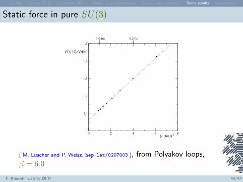
Static force in pure SU(3)

0 2 4 6 8(r [fm])-2

1

1.1

1.2

1.3

1.4

1.5

F(r) [GeV/fm]

1.0 fm 0.5 fm

[ M. Luscher and P. Weisz, hep-lat/0207003 ], from Polyakov loops,β = 6.0



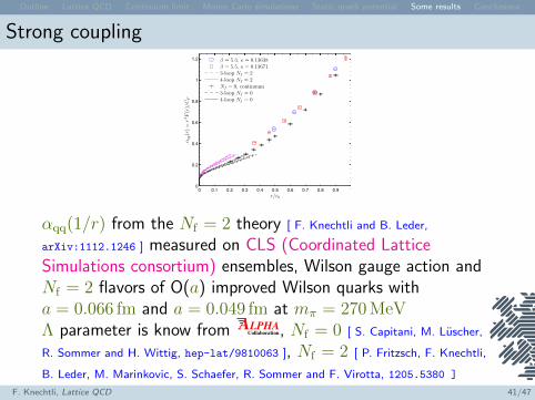
Strong coupling

0 0.1 0.2 0.3 0.4 0.5 0.6 0.7 0.8 0.9 10

0.2

0.4

0.6

0.8

1

1.2

r/r0

αqq(r)=

r2F(r)/C

F

β = 5.3, κ = 0.13638β = 5.5, κ = 0.136713-loop Nf = 24-loop Nf = 2Nf = 0, continuum3-loop Nf = 04-loop Nf = 0

αqq(1/r) from the Nf = 2 theory [ F. Knechtli and B. Leder,

arXiv:1112.1246 ] measured on CLS (Coordinated LatticeSimulations consortium) ensembles, Wilson gauge action andNf = 2 flavors of O(a) improved Wilson quarks witha = 0.066 fm and a = 0.049 fm at mπ = 270 MeVΛ parameter is know from LPHAA

Collaboration, Nf = 0 [ S. Capitani, M. Luscher,

R. Sommer and H. Wittig, hep-lat/9810063 ], Nf = 2 [ P. Fritzsch, F. Knechtli,

B. Leder, M. Marinkovic, S. Schaefer, R. Sommer and F. Virotta, 1205.5380 ]



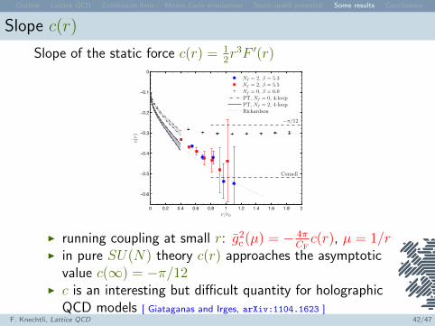
Slope c(r)

Slope of the static force c(r) = 12r3F ′(r)

0 0.2 0.4 0.6 0.8 1 1.2 1.4 1.6 1.8 2

−0.6

−0.5

−0.4

−0.3

−0.2

−0.1

0

r/r0

c(r)

Cornell

−π/12

Nf = 2, β = 5.3Nf = 2, β = 5.5Nf = 0, β = 6.0PT, Nf = 0, 4-loopPT, Nf = 2, 4-loopRichardson

I running coupling at small r: g2c (µ) = − 4π

CFc(r), µ = 1/r

I in pure SU(N) theory c(r) approaches the asymptoticvalue c(∞) = −π/12

I c is an interesting but difficult quantity for holographicQCD models [ Giataganas and Irges, arXiv:1104.1623 ]



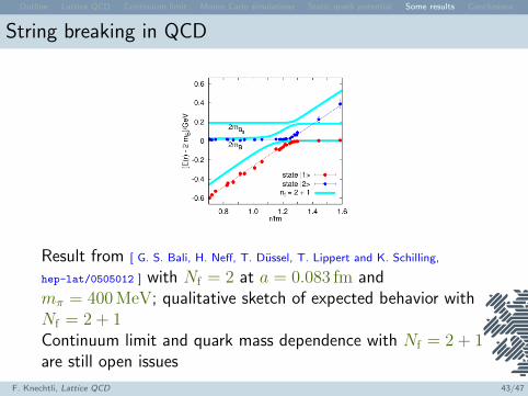
String breaking in QCD

Result from [ G. S. Bali, H. Neff, T. Dussel, T. Lippert and K. Schilling,

hep-lat/0505012 ] with Nf = 2 at a = 0.083 fm andmπ = 400 MeV; qualitative sketch of expected behavior withNf = 2 + 1Continuum limit and quark mass dependence with Nf = 2 + 1are still open issues



Hadro-quarkonium

Pentaquark

Candidates for a penta-quark state (ccuud) P+c (4380) (JP =

32

−) and P+

c (4450) (JP = 52

+) from Λb → J/ψ p K [ LHCb: R.

Aaij et al, 1507.03414, 1604.05708 ]

Hadro-quarkonia: quarkonia (cc) bound “within” ordinaryhadrons [ S. Dubynskiy and M. Voloshin, 0803.2224 ]

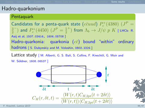
Lattice study [ M. Alberti, G. S. Bali, S. Collins, F. Knechtli, G. Moir and

W. Soldner, 1608.06537 ]

ttδ tδ

r

CH(r, δt, t) =〈W (r, t)CH,2pt(t+ 2δt)〉〈W (r, t)〉〈CH,2pt(t+ 2δt)〉



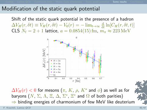
Modification of the static quark potential

Shift of the static quark potential in the presence of a hadron∆VH(r, δt) ≡ VH(r, δt)− V0(r) = − limt→∞

ddt

ln[CH(r, δt, t)]CLS Nf = 2 + 1 lattice, a = 0.0854(15) fm, mπ ≈ 223 MeV

0 0.1 0.2 0.3 0.4 0.5 0.6 0.7−5

−4

−3

−2

−1

0

r [fm]

∆Vπ(r)[M

eV]

π

δt = 2a

δt = 3a

δt = 4a

δt = 5a

δt = 6a

fit

∆VH(r) < 0 for mesons (π, K, ρ, K? and φ) as well as forbaryons (N , Σ, Λ, Ξ, ∆, Σ∗, Ξ∗ and Ω of both parities)⇒ binding energies of charmonium of few MeV like deuterium



Conclusions



Conclusions

I this lecture is a compact introduction to the formulationof QCD on the lattice discussing its continuum limit andMonte Carlo simulations

I the static quark potential is a quantity which shows theproperties of QCD from small to large distances and istherefore taken as an example

I more than 40 years after its invention, lattice field theoryhas developed into an active field of research connectingphysics, mathematics and informatics


Lattice Quantum Chromodynamics - Τομέας Φυσικήςphysik_uni-wuppertal... · Lattice...

Documents

Transcript of Lattice Quantum Chromodynamics - Τομέας Φυσικήςphysik_uni-wuppertal... · Lattice...