A NEW ADMM ALGORITHM FOR THE EUCLIDEAN MEDIAN AND ITS APPLICATION TOROBUST PATCH REGRESSION

Kunal N. Chaudhury K. R. Ramakrishnan

Department of Electrical Engineering, Indian Institute of Science, Bangalore, India

ABSTRACTThe Euclidean Median (EM) of a set of points Ω in an Euclideanspace is the point x minimizing the (weighted) sum of the Euclideandistances of x to the points in Ω. While there exits no closed-formexpression for the EM, it can nevertheless be computed using iterativemethods such as the Weiszfeld algorithm. The EM has classicallybeen used as a robust estimator of centrality for multivariate data. Itwas recently demonstrated that the EM can be used to perform robustpatch-based denoising of images by generalizing the popular Non-Local Means algorithm. In this paper, we propose a novel algorithmfor computing the EM (and its box-constrained counterpart) usingvariable splitting and the method of augmented Lagrangian. Theattractive feature of this approach is that the subproblems involved inthe ADMM-based optimization of the augmented Lagrangian can beresolved using simple closed-form projections. The proposed ADMMsolver is used for robust patch-based image denoising and is shownto exhibit faster convergence compared to an existing solver.

Index Terms— Image denoising, patch-based algorithm, robust-ness, Euclidean median, variable splitting, augmented Lagrangian,alternating direction method of multipliers (ADMM), convergence.

1. INTRODUCTION

Suppose we are given a set of points a1, . . . ,an ∈ Rd, and somenon-negative weights w1, . . . , wn to these points. Consider the prob-lem

minx∈C

n∑k=1

wk ‖x− ak‖2 (1)

where ‖·‖2 is the Euclidean norm and C ⊂ Rd is closed and convex.This is a convex optimization problem. The (global) minimizer of(1) when C is the entire space is called the Euclidean median (alsoreferred to as the geometric median) [1]. The Euclidean median hasclassically been used as a robust estimator of centrality for multivari-ate data [1]. This multivariate generalization of the scalar median alsocomes up in transport engineering, where (1) is used to model theproblem of locating a facility that minimizes the cost of transportation[2]. More recently, it was demonstrated in [3, 4] that the Euclideanmedian and its non-convex extensions can be used to perform robustpatch-based regression for image denoising by generalizing the poplarNon-Local Means algorithm [5, 6].

Note that the minimizer of (1) is simply the projection of theEuclidean median onto C. Unfortunately, there is no simple closed-form expression for the Euclidean median, even when it is unique [7].Nevertheless, the Euclidean median can be computed using numericalmethods such as the iteratively reweighted least squares (IRLS). Onesuch iterative method is the so-called Weiszfeld algorithm [8]. This

Correspondence: kunal@ee.iisc.ernet.in. The first author was partiallysupported by the Startup Grant provided by the Indian Institute of Science.

particular algorithm, however, is known to be prone to convergenceproblems [2]. Geometric optimization-based algorithms have also beproposed for approximating the Euclidean median [7]. More recently,motivated by the use of IRLS for sparse signal processing and L1

minimization [9, 10], an IRLS-based algorithm for approximatingthe Euclidean median was proposed in [3]. More precisely, here theauthors consider a smooth convex surrogate of (1), namely,

n∑k=1

wk (‖x− ak‖22 + ε)1/2 (ε > 0), (2)

and describe an iterative method for optimizing (2). The convergenceproperties of this iterative algorithm was later studied in [11].

In the last few years, there has been a lot of renewed interestin the use of variable splitting, the method of multipliers, and thealternating direction method of multipliers (ADMM) [12] for variousnon-smooth optimization problems in signal processing [13, 14, 15] .Motivated by this line of work, we introduce a novel algorithm forapproximating the solution of (1) using variable splitting and the aug-mented Lagrangian in Section 2. An important technical distinctionof the present approach is that, instead of working with the smoothsurrogate (2), we directly address the original non-smooth objectivein (1). The attractive feature here is that the subproblems involvedin the ADMM-based optimization of the augmented Lagrangian canbe resolved using simple closed-form projections. In Section 3, theproposed algorithm is used for robust patch-based denoising of im-ages following the proposal in [3]. In particular, we incorporate theinformation that the pixels of the original (clean) patches take val-ues in a given dynamic range (for example, in [0,255] for grayscaleimages) using an appropriately defined C. Numerical experimentsshow that the iterates of the proposed algorithm converge much morerapidly than the IRLS iterates for the denoising method in question.Moreover, the reconstruction quality of the denoised image obtainedafter few ADMM iterations is often substantially better than the IRLScounterpart.

2. EUCLIDEAN MEDIAN USING ADMM

Since we will primarily work with (1) in this paper, we will overloadterminology and refer to the minimizer of (1) as the Euclidean me-dian. The main idea behind the ADMM algorithm is to decomposethe objective in (1) into a sum of independent objectives, which canthen be optimized separately. This is precisely achieved using vari-able splitting [13, 14]. In particular, note that we can equivalentlyformulate (1) as

minz,x1,...,xn

ιC(z) +

n∑k=1

fk(xk)

subject to xk − z = 0 (k = 1, . . . , n),

(3)

arX

iv:1

501.

0387

9v1

[cs

.CV

] 1

6 Ja

n 20

15

wherefk(xk) = wk‖xk − ak‖2, (4)

and ιC is the indicator function of C [13]. In other words, we artifi-cially introduce one local variable for each term of the objective, anda common global variable that forces the local variables to be equal[16]. The advantage of this decomposition will be evident shortly.

Note that in the process of decomposing the objective, we haveintroduced additional constraints. While one could potentially useany of the existing constrained optimization methods to address (3),we will adopt the method of augmented Lagrangian which (amongother things) is particularly tailored to the separable structure of theobjective. The augmented Lagrangian for (3) can be written as

L = ιC(z) +

n∑k=1

fk(xk) + yTk (xk − z) +

µ

2‖xk − z‖22

(5)

where y1, . . . ,yn are the Lagrange multipliers corresponding to theequality constraints in (3), and µ > 0 is a penalty parameter [12, 13].

We next use the machinery of generalized ADMM to optimize Ljointly with respect to the variables and the Lagrange multipliers. Thegeneralized ADMM algorithm proceeds as follows [13, 16]: In eachiteration, we sequentially minimize L with respect to the variablesx1,x2, . . . ,xn,z in a Gauss-Seidel fashion (keeping the remain-ing variables fixed), and then we update the Lagrange multipliersy1, . . . ,yn using a fixed dual-ascent rule. In particular, note that theminimization over xk at the (t+ 1)-th iteration is given by

x(t+1)k = argmin

xfk(x) + (x− z(t))Ty

(t)k +

µ

2‖x− z(t)‖22 (6)

where z(t) denotes the variable z at the end of the t-th iteration. Asimilar notation is used to denote the Lagrange multipliers at the endof the t-th iteration.

Next, by combining the quadratic and linear terms and discardingterms that do not depend on z, we can express the partial minimiza-tion over z as

z(t+1) = argminz

ιC(z) +µ

2

N∑k=1

‖z − x(t+1)k − µ−1y

(t)k ‖

22

= argminz∈C

‖z − z(t+1)0 ‖22

where

z(t+1)0 =

1

N

N∑k=1

(x

(t+1)k + µ−1y

(t)k

).

Therefore,z(t+1) = PC(z

(t+1)0 ) (7)

where PC(x) denotes the projection of x onto the convex set C. Notethat we have used the most recent xk variables in (7). Finally, weupdate the Lagrange multipliers using the following standard rule:

y(t+1)k = y

(t)k + µ (x

(t+1)k − z(t+1)). (8)

We loop over (6), (7) and (8) until some convergence criteria ismet, or up to a fixed number of iterations. For a detailed expositionon the augmented Lagrangian, the method of multipliers, and theADMM, we refer the interested reader to [12, 13, 16].

We now focus on the update in (6). By combining the linear andquadratic terms (and discarding terms that do not depend on x), wecan express (6) in the following general form:

x? = argminx

f(x) +1

2‖x− v‖22 (9)

wheref(x) = λ ‖x− u‖2. (10)

Note that the objective in (9) is closed, proper, and strongly convex,and hence x? exists and is unique. In fact, we immediately recognizex? to be the proximal map of f evaluated at u [13, 17].

Definition 2.1 For any f : Rd 7→ (−∞,∞] that is closed, proper,and convex, the proximal map Ψf : Rd 7→ Rd is defined to be

Ψf (v) = argminx

f(x) +1

2‖x− v‖22 (v ∈ Rd). (11)

As per this definition, x? = Ψf (v).Note that (10) involves the L2 norm, which unlike the L1 norm

is not separable. A coordinate-wise minimization of (9) is thus notpossible (as is the case for the L1 norm leading to the well-knownshrinkage function). However, we have the following result on proxi-mal maps [13, 17].

Theorem 2.2 Let f : Rd 7→ (−∞,∞] be closed, proper, and con-vex. Then we can decompose any x ∈ Rd as

x = Ψf (x) + Ψf?(x), (12)

where f? : Rd 7→ (−∞,∞] is the convex conjugate of f ,

f?(y) = maxx

xTy − f(x) (y ∈ Rd). (13)

The usefulness of (12) is that both f? and and its proximal map canbe obtained in closed-form. Indeed, by change-of-variables,

f?(y) = maxx

xTy − λ ‖x− u‖2

= uTy + maxx

xTy − λ ‖x‖2.

Now, if ‖y‖2 ≤ λ, then by Cauchy-Schwarz, xTy ≤ λ ‖x‖2. Inthis case, the maximum over x is 0. On the other hand, if ‖y‖2 > λ,then setting x = ty (t > 0), we have

xTy − λ ‖x‖2 = t ‖y‖2 (‖y‖2 − λ) > 0,

which can be made arbitrarily large by letting t→∞. Thus,

f?(y) = uTy + ιB(y), (14)

where ιB is the indicator function of the ball B with centre 0 andradius λ,

ιB(y) =

0 if ‖y‖2 ≤ λ,∞ else.

Having obtained (14), we have from (11),

Ψf?(v) = argminx

uTx+ ιB(x) +1

2‖x− v‖22

= argminx∈B

1

2‖x− (v − u)‖22,

which is precisely the projection of v − u onto B. This is explicitlygiven by

Ψf?(v) = min(λ, ‖v − u‖2)v − u‖v − u‖2

. (15)

Combining (12) with (15), we have

Ψf (v) = Ψλ(v,u) = v −min(λ, ‖v − u‖2)v − u‖v − u‖2

. (16)

It is reassuring to note that Ψλ(v;u) equals v when λ = 0, andequals u when λ =∞. In the context of the ADMM update (6), notethat

λ = µ−1wk, u = ak, and v = z(t) − µ−1y(t)k .

The overall ADMM algorithm (called EM-ADMM) for computing theEuclidean median is summarized in Algorithm 1.

Data: Dimension d, points a1, . . . ,an ∈ Rd, and µ > 0.Result: z.Initialize: z,y1, . . . ,yn ∈ Rd;loop

r = 0;for k = 1, . . . , n do

xk = Ψµ−1wk(z − µ−1yk,ak);

r = r + xk + µ−1yk;endz = PC(N

−1r);for k = 1, . . . , n do

yk = yk + µ(xk − z);end

endAlgorithm 1: Euclidean Median using ADMM (EM-ADMM)

We next demonstrate how EM-ADMM can be used for robustpatch-based denoising of images. We also investigate its convergencebehavior in relation to the IRLS algorithm in [3].

3. APPLICATION: ROBUST PATCH REGRESSION

In the last ten years or so, some very effective patch-based algorithmsfor image denoising have been proposed [5, 18, 19, 20, 21]. One ofthe outstanding proposals in this area is the Non-Local Means (NLM)algorithm [5]. Several improvements and adaptations of NLM havebeen proposed since its inception, some of which currently offer state-of-the-art denoising results [21]. Recently, it was demonstrated in [3]that the denoising performance of NLM can be further improved byintroducing the robust Euclidean median into the NLM framework.

We consider the denoising setup where we are given a noisyimage g = (gi)i∈I (I is some linear ordering of the pixels in theimage) that is derived from some clean image f = (f i)i∈I via

gi = f i + σ ξi (i ∈ I),

where ξ = (ξi)i∈I is iidN (0, 1). The denoising problem is one ofestimating the unknown f from the noisy measurement g.

For any pixel i ∈ I , let patch Pi denote the restriction of g to asquare window centered at i. Letting k be the length of this window,this associates every pixel i with a patch-vector Pi of length k2. Fori, j ∈ I , define the weights wij = exp(−‖Pi −Pj‖22/h2), whereh > 0 is a smoothing parameter. For every i ∈ I , we consider thefollowing optimization problem

Pi = argminP∈Rk2

ιC(P) +∑j∈S(i)

wij‖P−Pj‖2. (17)

Here S(i) denotes the neighborhood pixels of i, namely, those pixelsthat are contained in a window of size S×S centred at i. The convexset C is defined to be the collection of patches whose pixel intensitiesare in the dynamic range [l, u]; e.g., l = 0 and u = 255 for a

1 2 3 4 5 6 7 8 9 1016

18

20

22

24

26

28

30

32

34

iterations

PS

NR

(d

B)

IRLS (sigma = 40)

ADMM (sigma = 40)

IRLS (sigma = 10)

ADMM (sigma = 10)

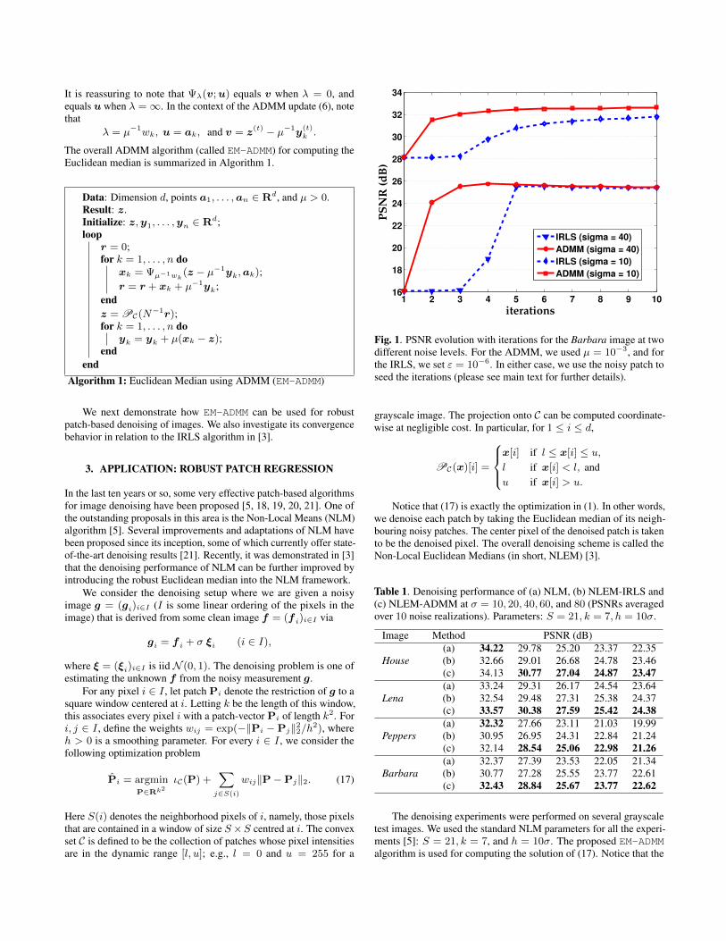
Fig. 1. PSNR evolution with iterations for the Barbara image at twodifferent noise levels. For the ADMM, we used µ = 10−3, and forthe IRLS, we set ε = 10−6. In either case, we use the noisy patch toseed the iterations (please see main text for further details).

grayscale image. The projection onto C can be computed coordinate-wise at negligible cost. In particular, for 1 ≤ i ≤ d,

PC(x)[i] =

x[i] if l ≤ x[i] ≤ u,l if x[i] < l, andu if x[i] > u.

Notice that (17) is exactly the optimization in (1). In other words,we denoise each patch by taking the Euclidean median of its neigh-bouring noisy patches. The center pixel of the denoised patch is takento be the denoised pixel. The overall denoising scheme is called theNon-Local Euclidean Medians (in short, NLEM) [3].

Table 1. Denoising performance of (a) NLM, (b) NLEM-IRLS and(c) NLEM-ADMM at σ = 10, 20, 40, 60, and 80 (PSNRs averagedover 10 noise realizations). Parameters: S = 21, k = 7, h = 10σ.

Image Method PSNR (dB)(a) 34.22 29.78 25.20 23.37 22.35

House (b) 32.66 29.01 26.68 24.78 23.46(c) 34.13 30.77 27.04 24.87 23.47(a) 33.24 29.31 26.17 24.54 23.64

Lena (b) 32.54 29.48 27.31 25.38 24.37(c) 33.57 30.38 27.59 25.42 24.38(a) 32.32 27.66 23.11 21.03 19.99

Peppers (b) 30.95 26.95 24.31 22.84 21.24(c) 32.14 28.54 25.06 22.98 21.26(a) 32.37 27.39 23.53 22.05 21.34

Barbara (b) 30.77 27.28 25.55 23.77 22.61(c) 32.43 28.84 25.67 23.77 22.62

The denoising experiments were performed on several grayscaletest images. We used the standard NLM parameters for all the experi-ments [5]: S = 21, k = 7, and h = 10σ. The proposed EM-ADMMalgorithm is used for computing the solution of (17). Notice that the

main computation here is that of determining the distances in (16).Since we require a total of S2 such distance evaluations in k2 dimen-sions, the complexity is O(S2k2) per iteration per pixel. Incidentally,this is also the complexity of the IRLS algorithm in [3]. For all thedenoising experiments, we initialized the Lagrange multipliers inEM-ADMM to zero vectors. We considered two possible initializationsfor z, namely, the noisy patch and the patch obtained using NLM.Exhaustive experiments showed that the best convergence results areobtained for µ ∼ 10−3. For example, figure 1 shows the evolutionof the peak-signal-to-noise ratio (PSNR) over the first ten iterationsobtained using the ADMM algorithm. Also show in this figure is theevolution of the PSNR for the IRLS algorithm from [3]. In eithercase, we used the noisy patch as the initialization. Notice that theincrease in PSNR is much more rapid with ADMM compared toIRLS. In fact, in about 4 iterations, the optimal PSNR is attained withADMM. Notice that at σ = 10, the PSNR from IRLS grows muchmore slowly compared to ADMM.

1 2 3 4 5 6 7 8 9 10

3.2

3.4

3.6

3.8

4

4.2

4.4

x 104

iterations

obje

ctiv

e fu

ncti

on(s

)

ADMMIRLSoptimal value

pixel of interest

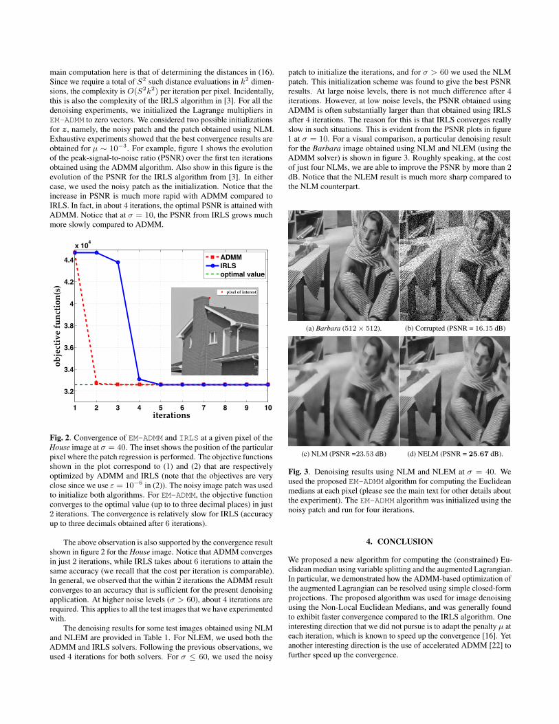
Fig. 2. Convergence of EM-ADMM and IRLS at a given pixel of theHouse image at σ = 40. The inset shows the position of the particularpixel where the patch regression is performed. The objective functionsshown in the plot correspond to (1) and (2) that are respectivelyoptimized by ADMM and IRLS (note that the objectives are veryclose since we use ε = 10−6 in (2)). The noisy image patch was usedto initialize both algorithms. For EM-ADMM, the objective functionconverges to the optimal value (up to to three decimal places) in just2 iterations. The convergence is relatively slow for IRLS (accuracyup to three decimals obtained after 6 iterations).

The above observation is also supported by the convergence resultshown in figure 2 for the House image. Notice that ADMM convergesin just 2 iterations, while IRLS takes about 6 iterations to attain thesame accuracy (we recall that the cost per iteration is comparable).In general, we observed that the within 2 iterations the ADMM resultconverges to an accuracy that is sufficient for the present denoisingapplication. At higher noise levels (σ > 60), about 4 iterations arerequired. This applies to all the test images that we have experimentedwith.

The denoising results for some test images obtained using NLMand NLEM are provided in Table 1. For NLEM, we used both theADMM and IRLS solvers. Following the previous observations, weused 4 iterations for both solvers. For σ ≤ 60, we used the noisy

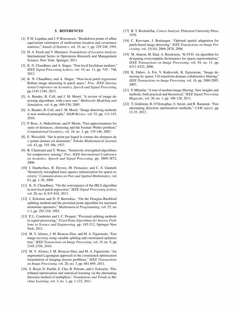
patch to initialize the iterations, and for σ > 60 we used the NLMpatch. This initialization scheme was found to give the best PSNRresults. At large noise levels, there is not much difference after 4iterations. However, at low noise levels, the PSNR obtained usingADMM is often substantially larger than that obtained using IRLSafter 4 iterations. The reason for this is that IRLS converges reallyslow in such situations. This is evident from the PSNR plots in figure1 at σ = 10. For a visual comparison, a particular denoising resultfor the Barbara image obtained using NLM and NLEM (using theADMM solver) is shown in figure 3. Roughly speaking, at the costof just four NLMs, we are able to improve the PSNR by more than 2dB. Notice that the NLEM result is much more sharp compared tothe NLM counterpart.

(a) Barbara (512× 512). (b) Corrupted (PSNR = 16.15 dB)

(c) NLM (PSNR =23.53 dB) (d) NELM (PSNR = 25.67 dB).

Fig. 3. Denoising results using NLM and NLEM at σ = 40. Weused the proposed EM-ADMM algorithm for computing the Euclideanmedians at each pixel (please see the main text for other details aboutthe experiment). The EM-ADMM algorithm was initialized using thenoisy patch and run for four iterations.

4. CONCLUSION

We proposed a new algorithm for computing the (constrained) Eu-clidean median using variable splitting and the augmented Lagrangian.In particular, we demonstrated how the ADMM-based optimization ofthe augmented Lagrangian can be resolved using simple closed-formprojections. The proposed algorithm was used for image denoisingusing the Non-Local Euclidean Medians, and was generally foundto exhibit faster convergence compared to the IRLS algorithm. Oneinteresting direction that we did not pursue is to adapt the penalty µ ateach iteration, which is known to speed up the convergence [16]. Yetanother interesting direction is the use of accelerated ADMM [22] tofurther speed up the convergence.

5. REFERENCES

[1] P. H. Lopuhaa and J. P. Rousseeuw, “Breakdown points of affineequivariant estimators of multivariate location and covariancematrices,” Annals of Statistics, vol. 19, no. 1, pp. 229-248, 1991.

[2] H. A. Eiselt and V. Marianov, Foundations of Location Analysis.International Series in Operations Research and ManagementScience, New York: Springer, 2011.

[3] K. N. Chaudhury and A. Singer, “Non-local Euclidean medians,”IEEE Signal Processing Letters, vol. 19, no. 11, pp. 745 - 748,2012.

[4] K. N. Chaudhury and A. Singer, “Non-local patch regression:Robust image denoising in patch space,” Proc. IEEE Interna-tional Conference on Acoustics, Speech and Signal Processing,pp.1345-1349, 2013.

[5] A. Buades, B. Coll, and J. M. Morel, “A review of image de-noising algorithms, with a new one,” Multiscale Modeling andSimulation, vol. 4, pp. 490-530, 2005.

[6] A. Buades, B. Coll, and J. M. Morel, “Image denoising methods.A new nonlocal principle,” SIAM Review, vol. 52, pp. 113-147,2010.

[7] P. Bose, A. Maheshwari, and P. Morin, “Fast approximations forsums of distances, clustering and the Fermat–Weber problem,”Computational Geometry, vol. 24, no. 3, pp. 135-146, 2003.

[8] E. Weiszfeld, “Sur le point par lequel le somme des distances den points donnes est minimum,” Tohoku Mathematical Journal,vol. 43, pp. 355-386, 1937.

[9] R. Chartrand and Y. Wotao, “Iteratively reweighted algorithmsfor compressive sensing,” Proc. IEEE International Conferenceon Acoustics, Speech and Signal Processing, pp. 3869-3872,2008.

[10] I. Daubechies, R. Devore, M. Fornasier, and C. S. Gunturk“Iteratively reweighted least squares minimization for sparse re-covery,” Communications on Pure and Applied Mathematics, vol.63, pp. 1-38, 2009.

[11] K. N. Chaudhury, “On the convergence of the IRLS algorithmin non-local patch regression,” IEEE Signal Processing Letters,vol. 20, no. 8, 815-818, 2013.

[12] J. Eckstein and D. P. Bertsekas, “On the Douglas-Rachfordsplitting method and the proximal point algorithm for maximalmonotone operators,” Mathematical Programming, vol. 55, no.1-3, pp. 293-318, 1992.

[13] P. L. Combettes and J. C. Pesquet, “Proximal splitting methodsin signal processing,” Fixed-Point Algorithms for Inverse Prob-lems in Science and Engineering, pp. 185-212, Springer NewYork, 2011.

[14] M. V. Afonso, J. M. Bioucas-Dias, and M. A. Figueiredo, “Fastimage recovery using variable splitting and constrained optimiza-tion,” IEEE Transactions on Image Processing, vol. 19, no. 9, pp.2345-2356, 2010.

[15] M. V. Afonso, J. M. Bioucas-Dias, and M. A. Figueiredo, “Anaugmented Lagrangian approach to the constrained optimizationformulation of imaging inverse problems,” IEEE Transactionson Image Processing, vol. 20, no. 3, pp. 681-695, 2011.

[16] S. Boyd, N. Parikh, E. Chu, B. Peleato, and J. Eckstein, “Dis-tributed optimization and statistical learning via the alternatingdirection method of multipliers,” Foundations and Trends in Ma-chine Learning, vol. 3, no. 1, pp. 1-122, 2011.

[17] R. T. Rockafellar, Convex Analysis. Princeton University Press,1970.

[18] C. Kervrann, J. Boulanger, “Optimal spatial adaptation forpatch-based image denoising,” IEEE Transactions on Image Pro-cessing, vol. 15(10), 2866-2878, 2006.

[19] M. Aharon, M. Elad, A. Bruckstein, “K-SVD: An algorithm fordesigning overcomplete dictionaries for sparse representation,”IEEE Transactions on Image Processing, vol. 54, no. 11, pp.4311-4322, 2006.

[20] K. Dabov, A. Foi, V. Katkovnik, K. Egiazarian, “Image de-noising by sparse 3-D transform-domain collaborative filtering,”IEEE Transactions on Image Processing, vol. 16, pp. 2080-2095,2007.

[21] P. Milanfar, “A tour of modern image filtering: New insights andmethods, both practical and theoretical,” IEEE Signal ProcessingMagazine, vol. 30, no. 1, pp. 106-128, 2013.

[22] T. Goldstein, B. O’Donoghue, S. Setzer, and R. Baraniuk, “Fastalternating direction optimization methods,” CAM report, pp.12-35, 2012.