Kernels

Nuno Vasconcelos ECE Department, UCSDp ,

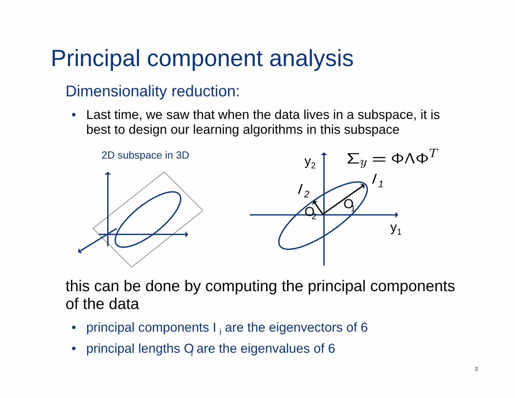
Principal component analysisDimensionality reduction:• Last time, we saw that when the data lives in a subspace, it is

best to design our learning algorithms in this subspace

2D subspace in 3D y2

φ

λ1λ2

φ1φ2

y1

this can be done by computing the principal components of the data

i i l t φ th i t f Σ

2

• principal components φi are the eigenvectors of Σ• principal lengths λi are the eigenvalues of Σ

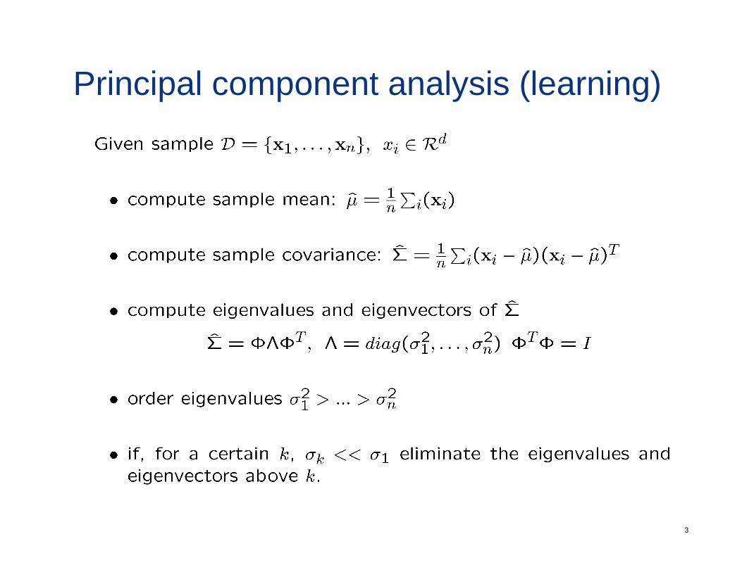
Principal component analysis (learning)

3

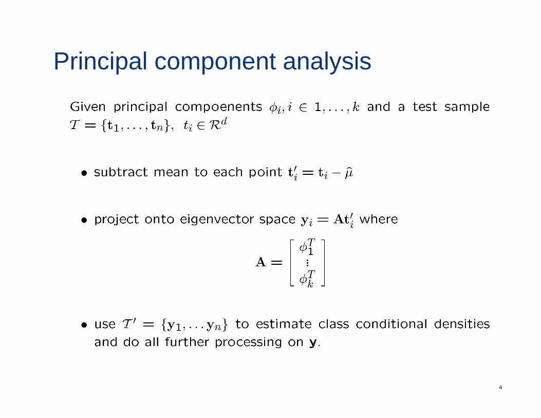
Principal component analysis

4

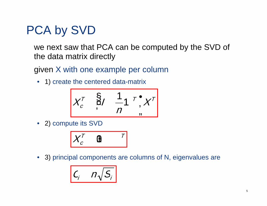
PCA by SVDwe next saw that PCA can be computed by the SVD of the data matrix directlygiven X with one example per column• 1) create the centered data-matrix

TTTc X

nIX ⎟

⎠⎞

⎜⎝⎛ −= 111

• 2) compute its SVD

TTcX ΜΠΝ=

• 3) principal components are columns of N, eigenvalues are

cX ΜΠΝ

5

ii n πλ =

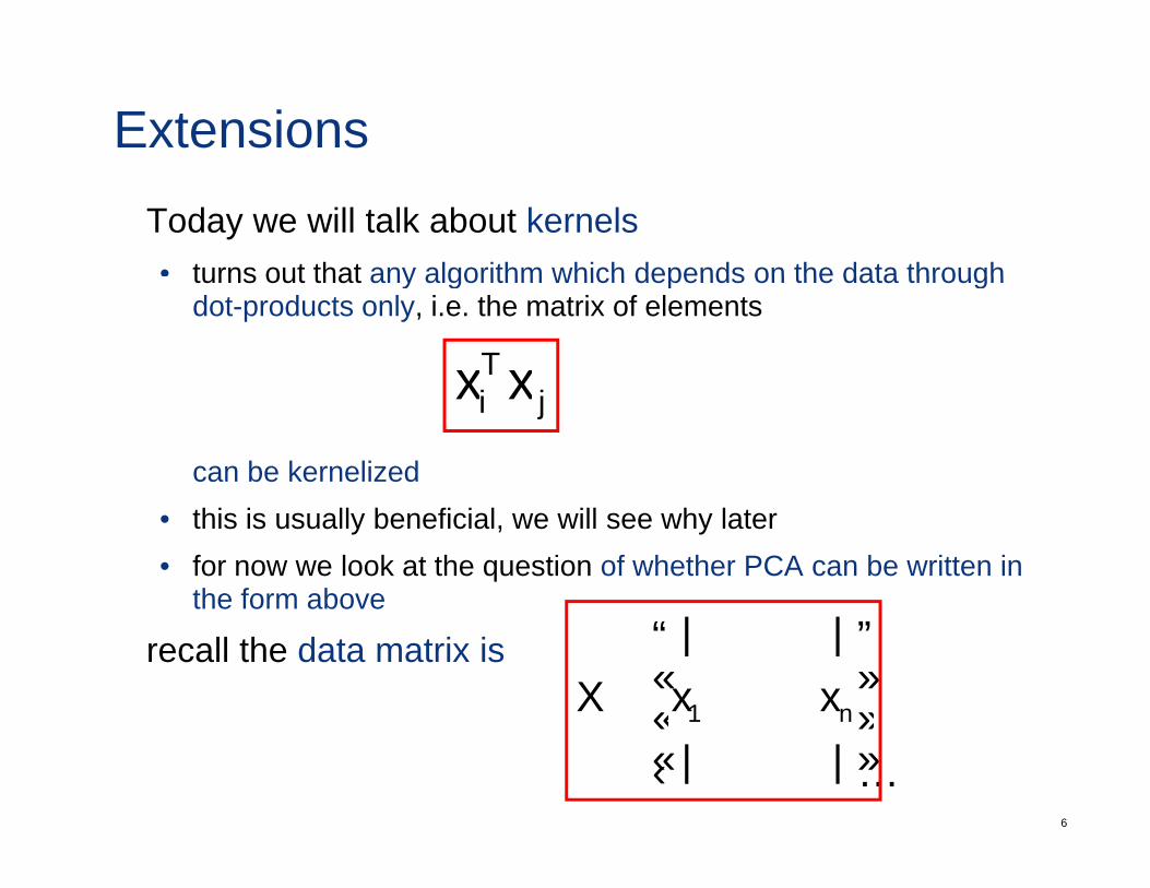
ExtensionsToday we will talk about kernels• turns out that any algorithm which depends on the data throughturns out that any algorithm which depends on the data through

dot-products only, i.e. the matrix of elements

T xxcan be kernelized

ji xx

• this is usually beneficial, we will see why later• for now we look at the question of whether PCA can be written in

the form above⎤⎡recall the data matrix is

⎥⎥⎤

⎢⎢⎡

=||

1 nxxX K

6

⎥⎥⎦⎢

⎢⎣ ||

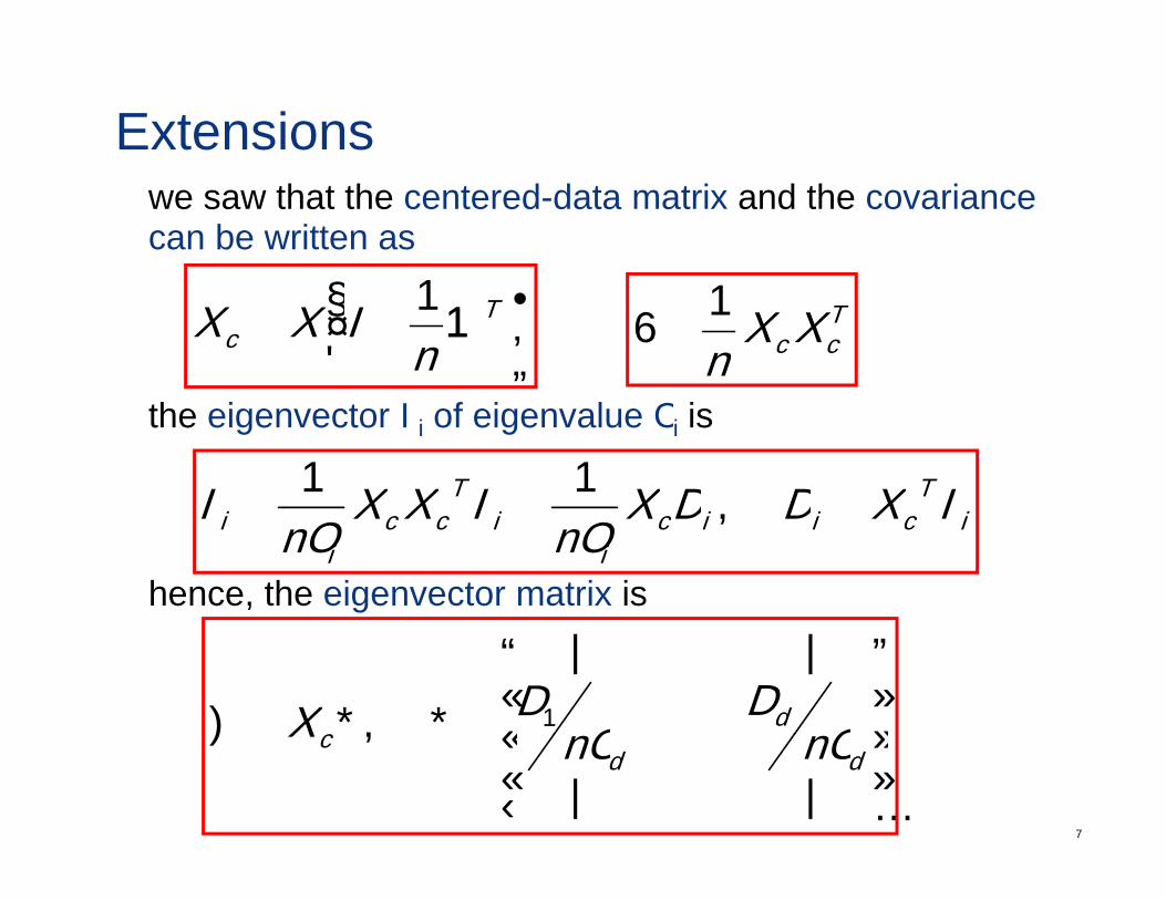
Extensionswe saw that the centered-data matrix and the covariance can be written as

⎞⎛⎟⎠⎞

⎜⎝⎛ −= T

c nIXX 111 T

cc XXn1

=Σ

the eigenvector φi of eigenvalue λi is

TT XXXX φααφφ ===11

hence, the eigenvector matrix is

iciici

icci

i XXn

XXn

φααλ

φλ

φ === ,

⎥⎥⎤

⎢⎢⎡

=ΓΓ=Φ

||

, 1 dcX λ

αλ

α K

7

⎥⎥

⎦⎢⎢

⎣

ΓΓΦ

||

,dd

c nnX λλ K

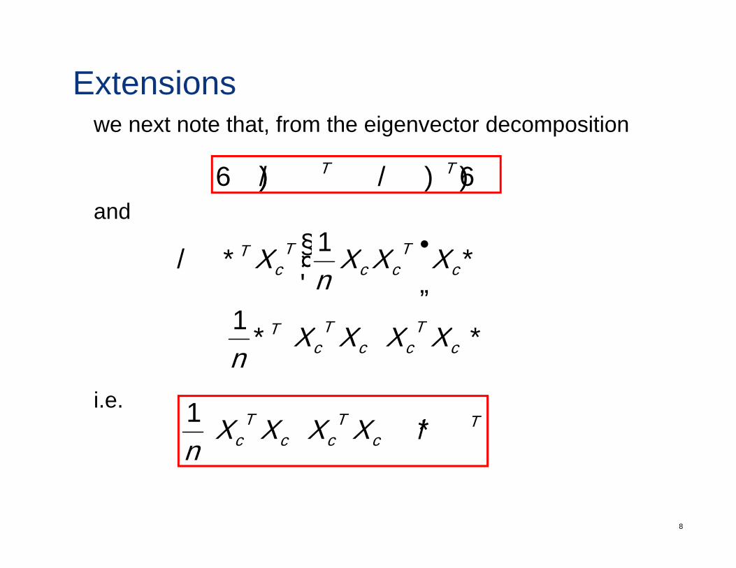
Extensionswe next note that, from the eigenvector decomposition

ΣΦΦ=Λ⇔ΦΛΦ=Σ TT

andΣΦΦ=Λ⇔ΦΛΦ=Σ

⎞⎜⎛ TTT 1

( )( )

Γ⎠⎞

⎜⎝⎛Γ=Λ c

Tcc

Tc

T XXXn

X

1

1

i

( )( )ΓΓ= cT

ccT

cT XXXX

n1

i.e.( )( ) T

cT

ccT

c XXXXn

ΓΛΓ=1

8

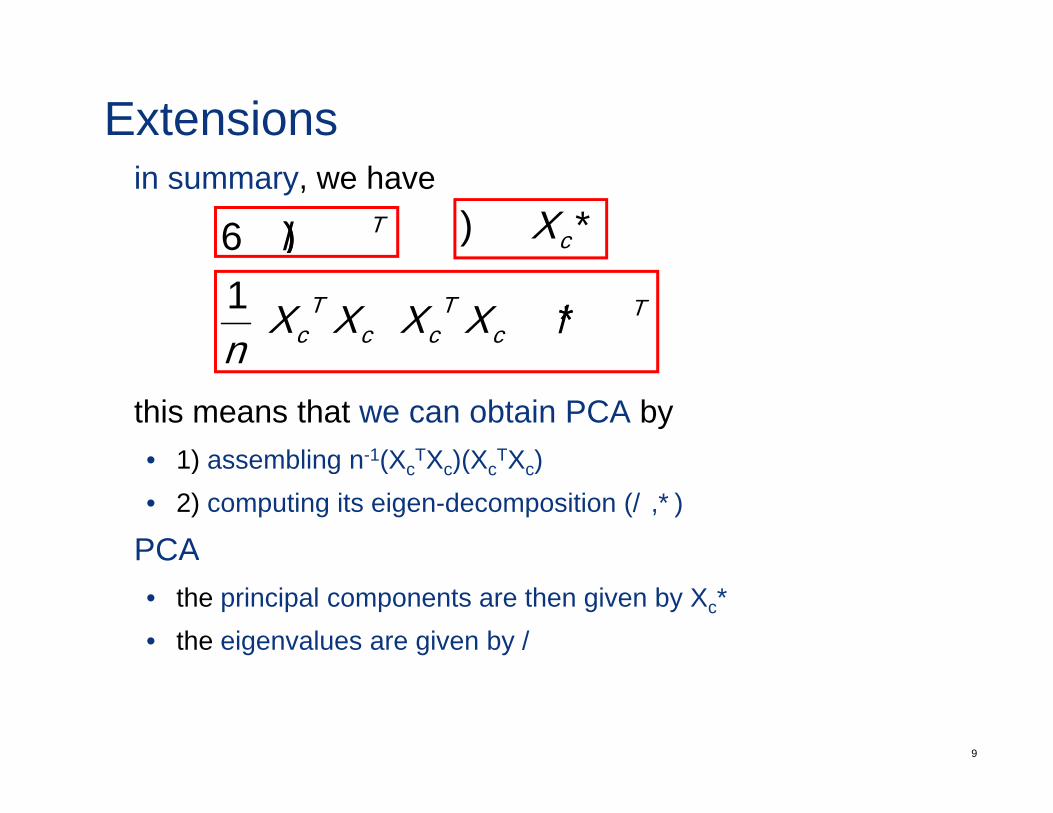
Extensionsin summary, we have

TΦΛΦ=Σ Γ=Φ cX

( )( ) Tc

Tcc

Tc XXXX

nΓΛΓ=

1

this means that we can obtain PCA by• 1) assembling n-1(X TX )(X TX )

n

• 1) assembling n 1(XcTXc)(Xc

TXc)• 2) computing its eigen-decomposition (Λ,Γ)

PCAC• the principal components are then given by XcΓ

• the eigenvalues are given by Λ

9

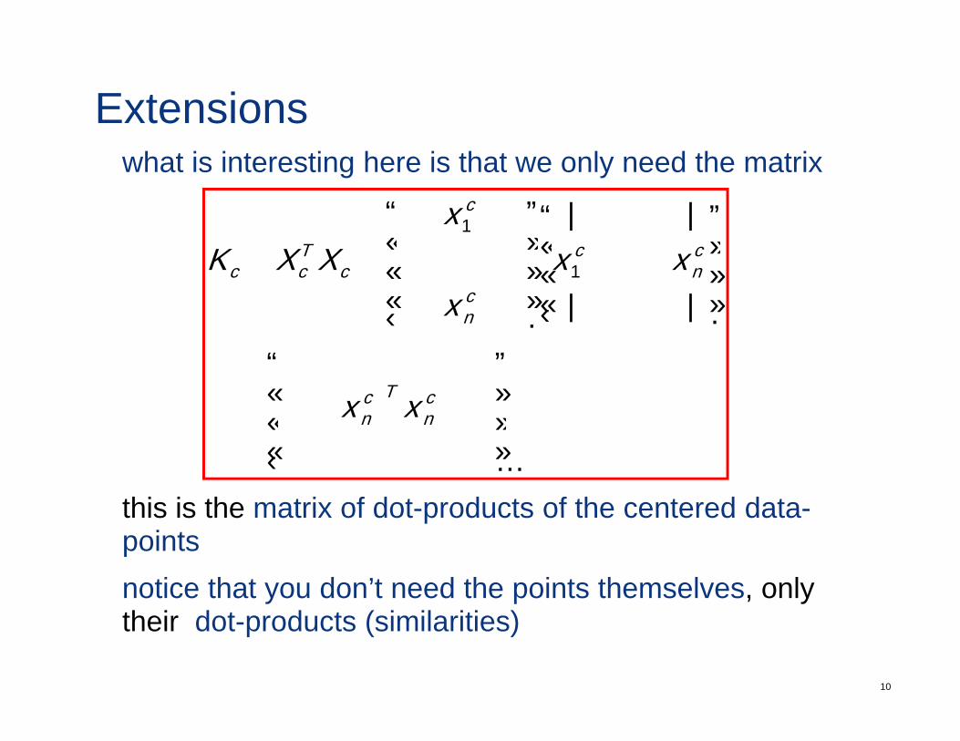
Extensionswhat is interesting here is that we only need the matrix

⎥⎤

⎢⎡

⎥⎤

⎢⎡ −− cx ||1

⎥⎥⎥

⎦⎢⎢⎢

⎣⎥⎥⎥

⎦⎢⎢⎢

⎣ −−== KM c

nc

cn

cTcc xx

xXXK

||

||

1

1

( ) ⎥⎥⎤

⎢⎢⎡

=

⎦⎣⎦⎣

KK

Mcn

Tcn xx

this is the matrix of dot-products of the centered data-

( )⎥⎥⎦⎢

⎢⎣ M

KK nn

this is the matrix of dot-products of the centered data-pointsnotice that you don’t need the points themselves, only

10

their dot-products (similarities)

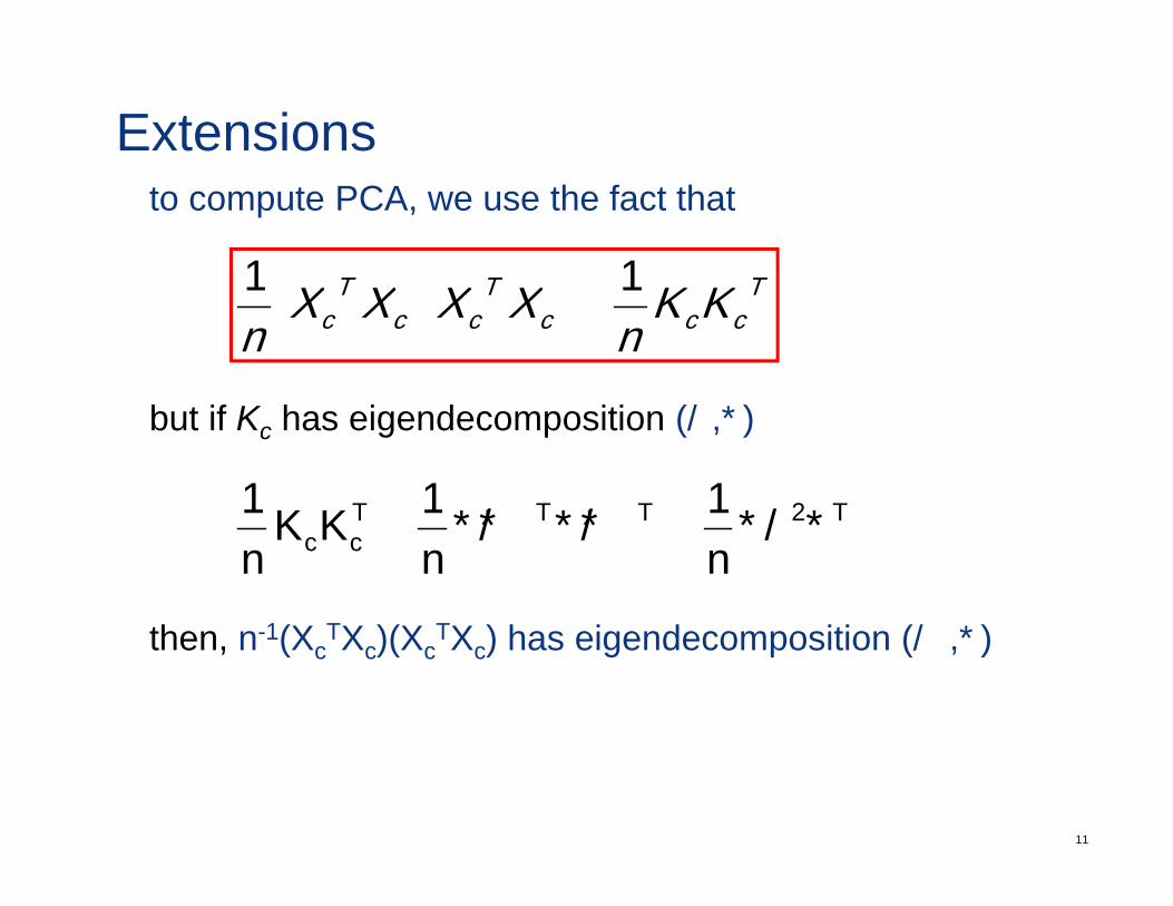
Extensionsto compute PCA, we use the fact that

( )( ) TTT 11 ( )( ) Tccc

Tcc

Tc KK

nXXXX

n11

=

but if Kc has eigendecomposition (Λ,Γ)

TTTT 2111

h 1(X TX )(X TX ) h i d i i ( 2 )

TTTTcc nn

KKn

ΓΓΛ=ΓΛΓΓΛΓ= 2111

then, n-1(XcTXc)(Xc

TXc) has eigendecomposition (Λ2,Γ)

11

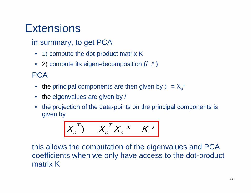
Extensionsin summary, to get PCA• 1) compute the dot-product matrix K• 2) compute its eigen-decomposition (Λ,Γ)

PCAth i i l t th i b Φ X Γ• the principal components are then given by Φ = XcΓ

• the eigenvalues are given by Λ2

• the projection of the data-points on the principal components isthe projection of the data points on the principal components is given by

Γ=Γ=Φ KXXX cT

cT

c

this allows the computation of the eigenvalues and PCA coefficients when we only have access to the dot-product

ccc

12

coefficients when we only have access to the dot product matrix K

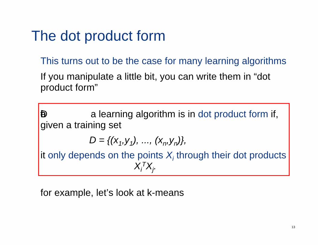
The dot product formThis turns out to be the case for many learning algorithmsIf you manipulate a little bit you can write them in “dotIf you manipulate a little bit, you can write them in dot product form”

Definition: a learning algorithm is in dot product form if, given a training set

D {( ) ( )}D = {(x1,y1), ..., (xn,yn)},it only depends on the points Xi through their dot products

XiTXj.Xi Xj.

for example, let’s look at k-means

13

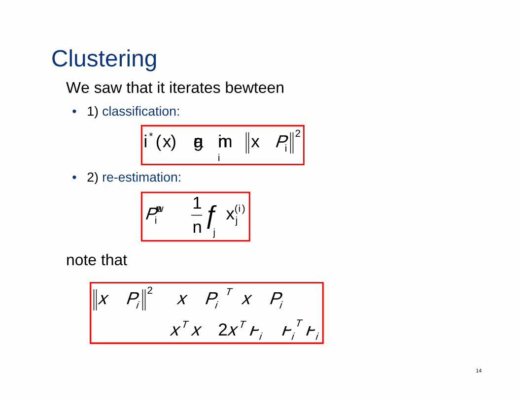
ClusteringWe saw that it iterates bewteen• 1) classification:

2) re estimation:

2* minarg)( ii

xxi µ−=

• 2) re-estimation:

∑= ij

newi x

n)(1µ

note that

∑j

jn

( ) ( )TTT

iT

ii

xxx

xxx µµµ −−=−

2

2

14

iT

iiTT xxx µµµ +−= 2

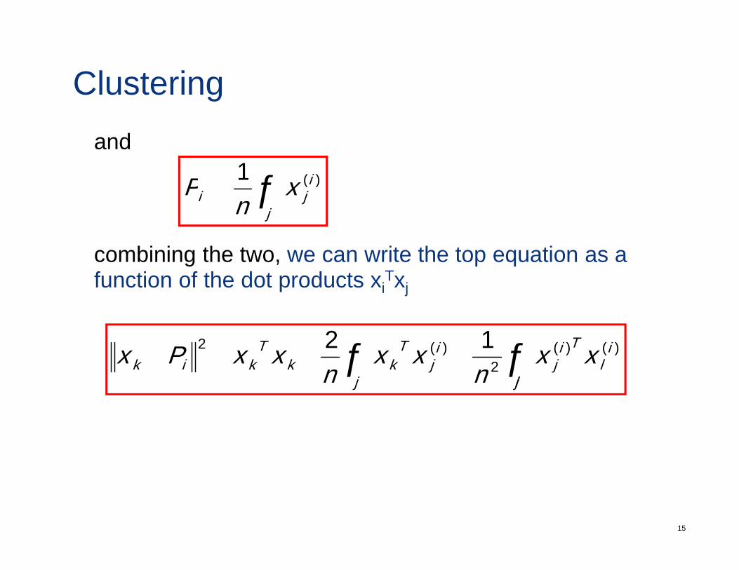
Clusteringand

∑ i )(1

bi i th t it th t ti

∑=j

iji x

n)(1µ

combining the two, we can write the top equation as a function of the dot products xi

Txj

∑∑ +−=−jl

il

Tij

j

ij

Tkk

Tkik xx

nxx

nxxx )()(

2)(2 12 µ

15

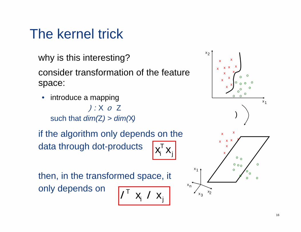
The kernel trickwhy is this interesting?consider transformation of the feature

xx

x

xx

x

x

x2

consider transformation of the featurespace:• introduce a mapping

xx

x

xx

xo

oo

o

o

ooo

ooo

o

x1pp g

Φ: X → Zsuch that dim(Z) > dim(X)

if th l ith l d d th

x1

Φ

if the algorithm only depends on thedata through dot-products

xx

x

x

x

xx

x

xx

x

x

o oj

Ti xx

then, in the transformed space, it only depends on

xo

oo

o

o oo

o oo

ox1

xn

( ) ( )16

only depends onx3

x2( ) ( )jiT xx φφ

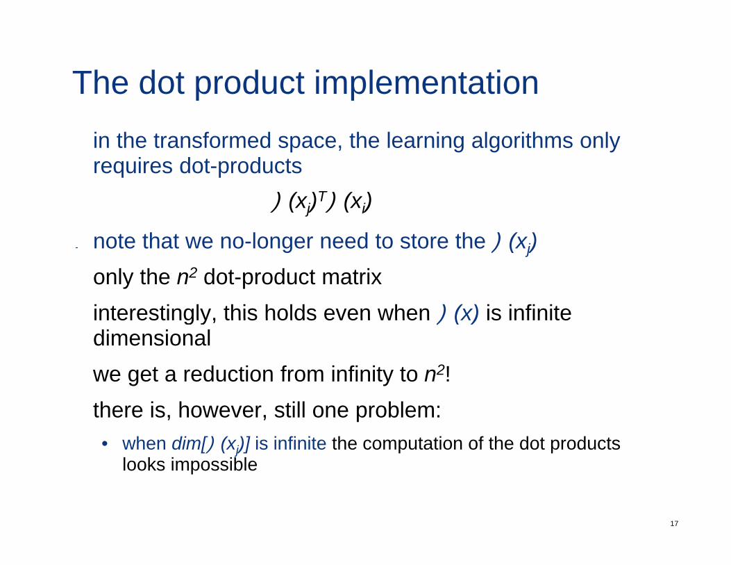
The dot product implementationin the transformed space, the learning algorithms only requires dot-productsq p

Φ(xj)TΦ(xi)

note that we no-longer need to store the Φ(xj)note that we no longer need to store the Φ(xj)only the n2 dot-product matrixinterestingly, this holds even when Φ(x) is infiniteinterestingly, this holds even when Φ(x) is infinite dimensional we get a reduction from infinity to n2!there is, however, still one problem:• when dim[Φ(xj)] is infinite the computation of the dot products

looks impossible

17

looks impossible

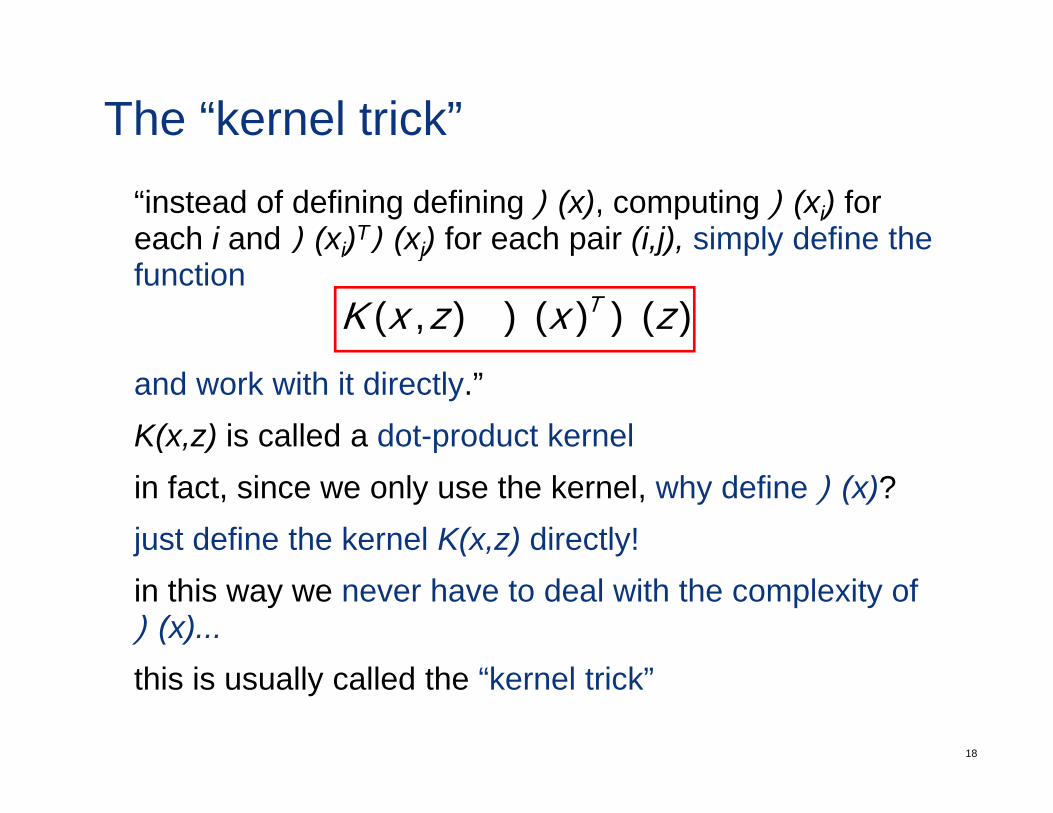
The “kernel trick”“instead of defining defining Φ(x), computing Φ(xi) for each i and Φ(xi)TΦ(xj) for each pair (i,j), simply define the ( i) ( j) p ( ,j), p yfunction

)()(),( zxzxK T ΦΦ=

and work with it directly.”K(x,z) is called a dot-product kernelin fact, since we only use the kernel, why define Φ(x)?just define the kernel K(x,z) directly!in this way we never have to deal with the complexity of Φ(x)...

18

this is usually called the “kernel trick”

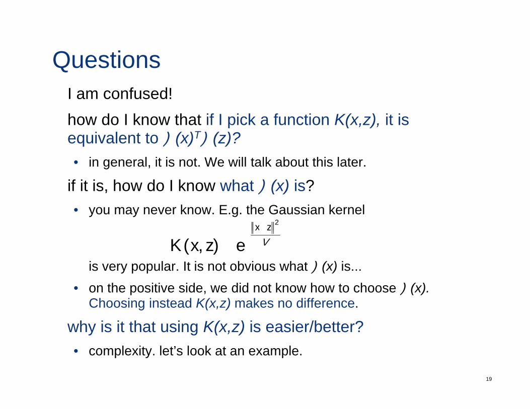
QuestionsI am confused!how do I know that if I pick a function K(x,z), it is p ( , ),equivalent to Φ(x)TΦ(z)?• in general, it is not. We will talk about this later.

if it is, how do I know what Φ(x) is?• you may never know. E.g. the Gaussian kernel

2zx−

is very popular. It is not obvious what Φ(x) is...

σ),(x

ezxK−

=

• on the positive side, we did not know how to choose Φ(x).Choosing instead K(x,z) makes no difference.

why is it that using K(x,z) is easier/better?

19

y g ( , )• complexity. let’s look at an example.

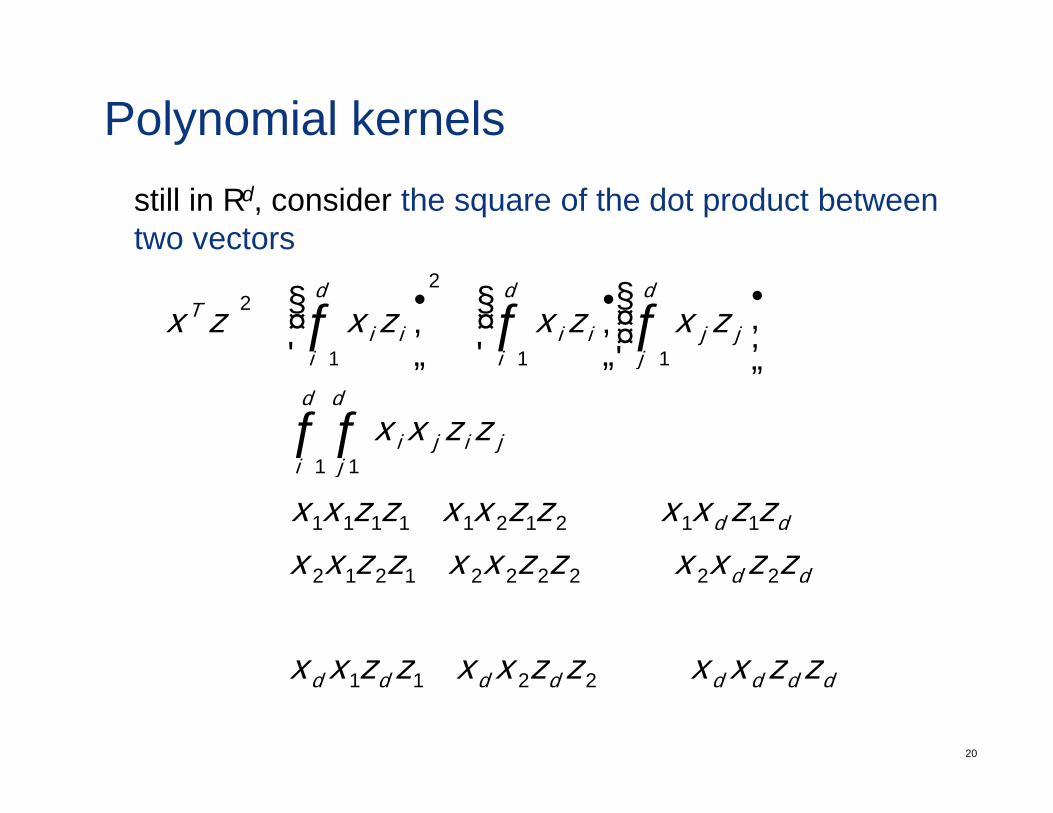
Polynomial kernelsstill in Rd, consider the square of the dot product between two vectors

( )d

jjj

d

iii

d

iii

T zxzxzxzx =⎟⎟⎠

⎞⎜⎜⎝

⎛⎟⎠

⎞⎜⎝

⎛=⎟

⎠

⎞⎜⎝

⎛= ∑∑∑

11

2

1

2

d d

jiji

jii

zzxx=

⎠⎝⎠⎝⎠⎝

∑∑

=== 111

dd

i j

zzxxzzxxzzxxzzxxzzxxzzxx

+++++++++=

= =

K 1121211111

1 1

dd

zzxxzzxxzzxx

zzxxzzxxzzxx

++++

+++++M

K 2222221212

20

dddddddd zzxxzzxxzzxx ++++ K2211

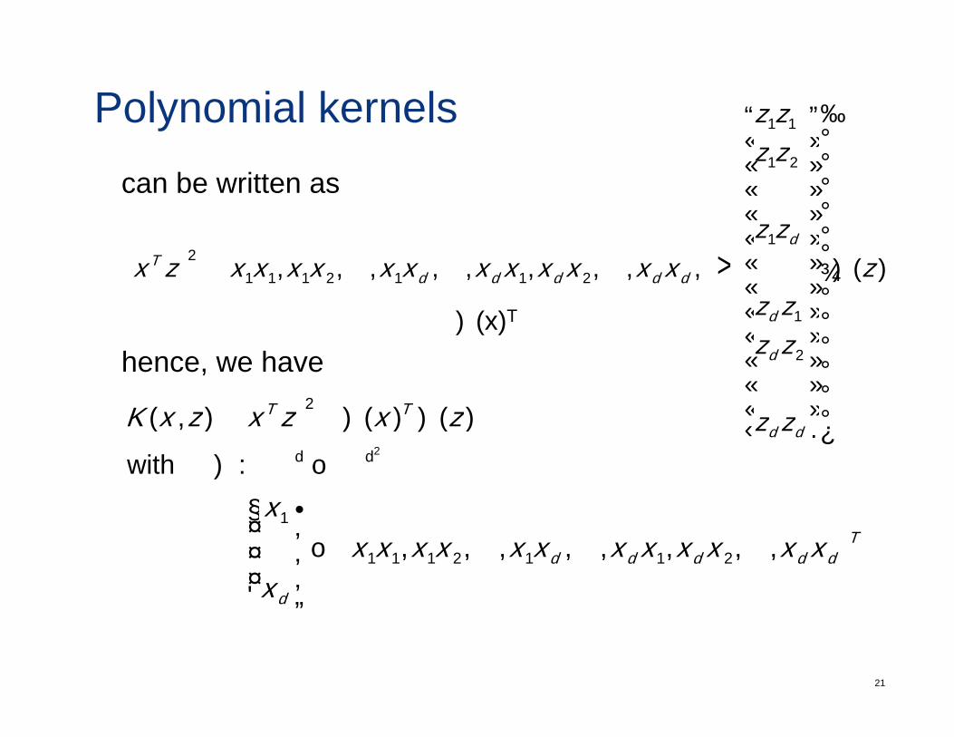
Polynomial kernels 11zz⎪⎫

⎥⎤

⎢⎡

can be written as21

zz

zz

⎪⎪⎪⎪⎪

⎥⎥⎥⎥⎥

⎢⎢⎢⎢⎢

M

( ) [ ] )(,,,,,,,,,

1

1

21121112 z

zz

zzxxxxxxxxxxxxzx

d

d

dddddT Φ

⎪⎪

⎪⎪⎬

⎥⎥⎥⎥⎥

⎢⎢⎢⎢⎢

= M444444444 3444444444 21KKKK

Φ(x)T

hence, we have 2zzd

⎪⎪⎪⎪⎪

⎥⎥⎥⎥

⎦⎢⎢⎢⎢

⎣

M

Φ(x)

( ) TT zxzxzxK )()()( 2ΦΦ zz dd ⎪⎭

⎥⎦

⎢⎣( )

x

zxzxzxK )()(),(

⎞⎛

ℜ→ℜΦ

ΦΦ==

: with2dd

( )Tddddd

d

xxxxxxxxxxxxx

x,,,,,,,, 2112111

1

LLLM →⎟⎟⎟

⎠

⎞

⎜⎜⎜

⎝

⎛

21

d ⎠⎝

Polynomial kernelsthe point is that• while Φ(x)TΦ(z) has complexity O(d2)• while Φ(x) Φ(z) has complexity O(d )• direct computation of K(x,z) = (xTz)2 has complexity O(d)

direct evaluation is more efficient by a factor of dyas d goes to infinity this makes the idea feasibleBTW, you just met another kernel family, y j y• this implements polynomials of second order• in general, the family of polynomial kernels is defined as

I d ’t t t thi k b t iti d Φ( ) !

( ) { }L,2,1,1),( ∈+= kzxzxK kT

22

• I don’t even want to think about writing down Φ(x) !

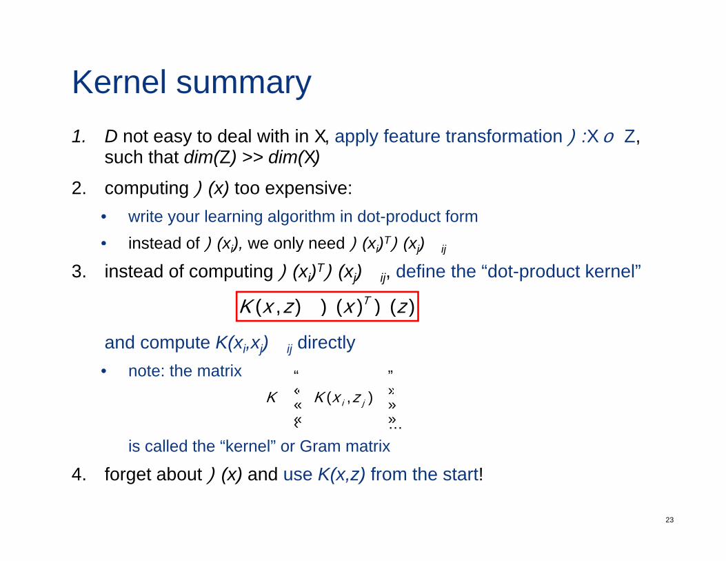
Kernel summary1. D not easy to deal with in X, apply feature transformation Φ:X → Z,

such that dim(Z) >> dim(X)

2. computing Φ(x) too expensive:• write your learning algorithm in dot-product form• instead of Φ(xi) we only need Φ(xi)TΦ(xj) ∀ijinstead of Φ(xi), we only need Φ(xi) Φ(xj) ∀ij

3. instead of computing Φ(xi)TΦ(xj) ∀ij, define the “dot-product kernel”

)()(),( zxzxK T ΦΦ=

and compute K(xi,xj) ∀ij directly• note: the matrix

)()()(

⎥⎤

⎢⎡ M

is called the “kernel” or Gram matrix

⎥⎥⎥

⎦⎢⎢⎢

⎣

=M

LL ),( ji zxKK

23

4. forget about Φ(x) and use K(x,z) from the start!

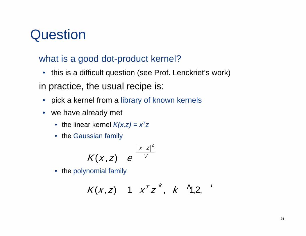
Questionwhat is a good dot-product kernel?• this is a difficult question (see Prof Lenckriet’s work)this is a difficult question (see Prof. Lenckriet s work)

in practice, the usual recipe is:• pick a kernel from a library of known kernelsp y• we have already met

• the linear kernel K(x,z) = xTz• the Gaussian family

σ

2

),(zx

ezxK−

−=

• the polynomial family

)(

( ) { }L,2,1,1),( ∈+= kzxzxK kT

24

( ) { },2,1,1),( ∈+ kzxzxK

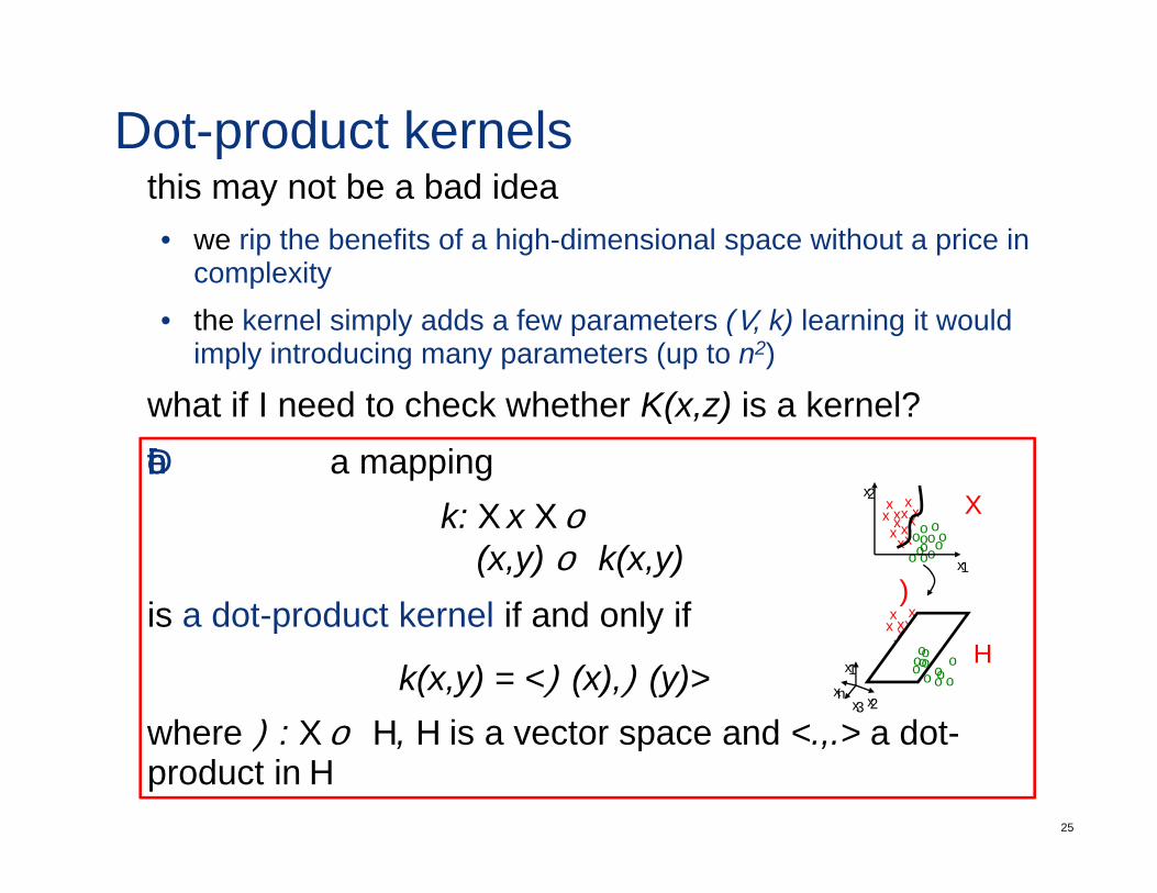
Dot-product kernelsthis may not be a bad idea• we rip the benefits of a high-dimensional space without a price in

complexitycomplexity• the kernel simply adds a few parameters (σ, k) learning it would

imply introducing many parameters (up to n2)

what if I need to check whether K(x,z) is a kernel? Definition: a mapping

k xxx2 Xk: X x X → ℜ

(x,y) → k(x,y)is a dot product kernel if and only if

xxx

xx

xxx

xxxx

ooo

ooooo

oooo

x1

xxΦ

X

is a dot-product kernel if and only if

k(x,y) = <Φ(x),Φ(y)>where Φ: X → H H is a vector space and < > a dot

xxx

xx

xxx

xxxx

oo o

ooo oo

o ooox1

x3 x2xn

H

25

where Φ: X → H, H is a vector space and <.,.> a dot-product in H

Positive definite matricesrecall that (e.g. Linear Algebra and Applications, Strang)

Definition: each of the following is a necessary andDefinition: each of the following is a necessary and sufficient condition for a real symmetric matrix A to be (semi) positive definite:

i) TA ≥ 0 0i) xTAx ≥ 0, ∀ x ≠ 0 ii) all eigenvalues of A satisfy λi ≥ 0iii) all upper-left submatrices Ak have non-negative determinanti ) there is a matri R ith independent ro s s ch thativ) there is a matrix R with independent rows such that

A = RTR

l ft b t iupper left submatrices:

L 322212

3,12,11,1

32,11,1

2111 ⎥⎥⎤

⎢⎢⎡

=⎥⎤

⎢⎡

== aaaaaa

Aaa

AaA

26

3,32,31,3

3,22,21,232,21,2

21,11

⎥⎥⎦⎢

⎢⎣

⎥⎦

⎢⎣ aaa

aa

Positive definite matricesproperty iv) is particularly interesting• in ℜ d <x x> = xTAx is a dot-product kernel if and only if A is• in ℜ , <x,x> = x Ax is a dot-product kernel if and only if A is

positive definite• from iv) this holds if and only if there is R such that A = RTR• hence

<x,y> = xTAy = (xR)T(Ry) = Φ(x)TΦ(y)with

Φ: ℜ d → ℜ d

x → Rx

i.e. the dot-product kernelp

k(x,z) = xTAz, (A positive definite)is the standard dot-product in the range space of the

27

is the standard dot product in the range space of the mapping Φ(x) = Rx

Positive definite kernelshow do I extend this notion of positive definiteness to functions?Definition: a function k(x,y) is a positive definite kernel on X xX if ∀ l and ∀ {x1, ..., xl}, xi∈ X, the Gram matrix

⎥⎥⎤

⎢⎢⎡

= LL

M

),( ji xxkK

is positive definite.

⎥⎥⎦⎢

⎢⎣ M

),( ji

plike in in ℜ d, this allows us to check that we have a positive definite kernel

28

Dot product kernelsTheorem: k(x,y), x,y∈ X, is a dot-product kernel if and only if it is a positive definite kernely pin summary, to check whether a kernel is a dot product:• check if the Gram matrix is positive definite • for all possible sequences {x1, ..., xl}, xi∈ X

does the kernel have to be a dot-product kernel?not necessarily. For example, neural networks can be seen as implementing kernels that are not of this typehhowever:• you loose the parallelism. what you know about the learning

machine may no longer hold after you kernelize

29

• dot-product kernels usually lead to convex learning problems. Usually you loose this guarantee for non dot-product

Clusteringso far, this is mostly theoreticalhow does it affect my algorithms?consider, for example, the k-means algorithm• 1) classification:

2) ti ti

2* minarg)( ii

xxi µ−=

• 2) re-estimation:

∑= ij

newi x )(1µ

can we kernelize the classification step?

∑j

jn

30

Clusteringwell, we saw that

T2 12

thi th b k li d i t

∑∑ +−=−jl

il

Tij

j

ij

Tkk

Tkik xx

nxx

nxxx )()(

2)(2 12 µ

this can then be kernelized into

( ) ( ) ( ) ( )∑ ΦΦ−ΦΦ=− ij

Tkk

Tkik xxxxx )(2 2µ ( ) ( ) ( ) ( )

( ) ( )∑

∑

ΦΦ+ il

Tij

jjkkkik

xx

n

)()(2

1

µ

( ) ( )∑jl

ljn 2

31

Clusteringfurthermore, this can be done with relative efficiency

( ) ( ) ( ) ( )∑ ΦΦΦΦ= iTT xxxxx )(2 2µ ( ) ( ) ( ) ( )

( ) ( )∑

∑

ΦΦ+

ΦΦ−ΦΦ=−

iTi

jjkkkik

xx

xxn

xxx

)()(1

µ

( ) ( )∑ ΦΦ+jl

lj xxn

)()(2

the assignment of the point only requires computing

kth diagonal entry of Gram matrix computed once per clusterwhen all points are assigned

( )2requires computing for each clusterthis is a sum of entries of Gram

( ) ( )∑ ΦΦj

ij

Tk xx

n)(2

32

this is a sum of entries of Grammatrix

Clusteringnote, however, that we cannot explicitly compute

1

thi i b bl i fi it di i l

( ) ( )∑Φ=Φj

iji x

n)(1µ

this is probably infinite dimensional...in any case, if we define

a Gram matrix K(i) for each cluster (dot products between points• a Gram matrix K(i) for each cluster (dot products between points in cluster)

• and S(i) the scaled sum of the entries in this matrix

( ) ( )∑ ΦΦ=jl

il

Tij

i xxn

S )()(2

)( 1

33

jl

Clusteringwe obtain the kernel k-means algorithm• 1) classification:1) classification:

( ) ( )⎥⎤⎢⎡

ΦΦ−+= ∑ ij

Tl

illl xxSKxi )()(* 2minarg)(

• 2) re-estimation: update

( ) ( )⎥⎦

⎢⎣

∑j

jllli

l n,g)(

) p

( ) ( )∑ ΦΦ=jl

il

Tij

i xxn

S )()(2

)( 1

but we no longer have access to the prototype for each cluster

jln

34

Clusteringwith the right kernel this can work significantly better than regular k-meansg

k-meanskernel

k-means

Φ

35

Clusteringbut for other applications, where the prototypes are important, this may be uselessp , ye.g. compression

we can try replacing the prototype by the closest vector, but this is not necessarily optimal

36

PCAwe saw that, to get PCA• 1) compute the dot-product matrix K• 2) compute its eigen-decomposition (Λ,Γ)

PCAth i i l t th i b Φ X Γ• the principal components are then given by Φ = XcΓ

• the eigenvalues are given by Λ2

• the projection of the data-points on the principal components isthe projection of the data points on the principal components is given by

Γ=Φ KX Tc

note that most of this holds when we kernelize, we only have to change the matrix K from xi

Txj to φ(xi)Tφ(xj)th l thi l th PC X

37

• the only thing we can no longer access are the PCs Φ = XcΓ

Kernel methodsmost learning algorithms can be kernelized• kernel PCAkernel PCA• kernel LDA• kernel ICA,• etc.

as in k-means, sometimes we loose some of the features of the original algorithmof the original algorithmbut the performance is frequently betternext week we will look at the canonical application thenext week we will look at the canonical application, the support vector machine

38

39