Inverse Reinforcement Learning - University of …pabbeel/cs287-fa12/...High-level picture Dynamics...
75
Inverse Reinforcement Learning Pieter Abbeel UC Berkeley EECS
Transcript of Inverse Reinforcement Learning - University of …pabbeel/cs287-fa12/...High-level picture Dynamics...
Inverse Reinforcement Learning
Pieter Abbeel
UC Berkeley EECS
Inverse Reinforcement Learning
[equally good titles: Inverse Optimal Control,[equally good titles: Inverse Optimal Control,
Inverse Optimal Planning]
Pieter Abbeel
UC Berkeley EECS
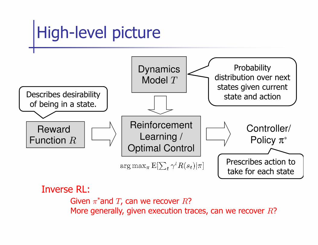
High-level picture
Dynamics Model T
Reinforcement
Probability distribution over next states given current
state and actionDescribes desirability of being in a state.
Reward Function R
Reinforcement
Learning /
Optimal Control
Controller/
Policy π∗
Prescribes action to take for each state
Inverse RL: Given π*and T, can we recover R?More generally, given execution traces, can we recover R?
� Scientific inquiry
� Model animal and human behavior
� E.g., bee foraging, songbird vocalization. [See intro of Ng and Russell, 2000 for a brief overview.]
� Apprenticeship learning/Imitation learning through
Motivation for inverse RL
Apprenticeship learning/Imitation learning through inverse RL
� Presupposition: reward function provides the most succinct and transferable definition of the task
� Has enabled advancing the state of the art in various robotic domains
� Modeling of other agents, both adversarial and cooperative

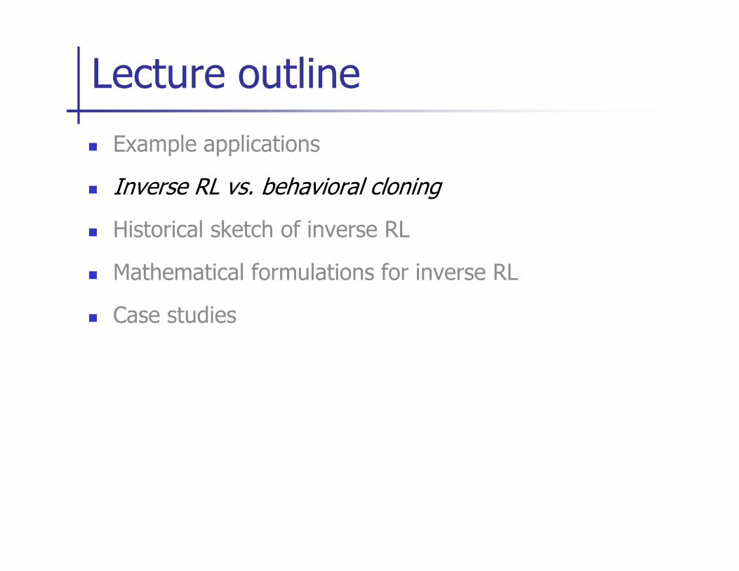
� Example applications
� Inverse RL vs. behavioral cloning
� Historical sketch of inverse RL
� Mathematical formulations for inverse RL
Lecture outline
� Case studies
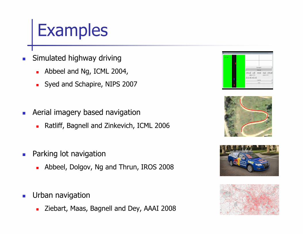
� Simulated highway driving
� Abbeel and Ng, ICML 2004,
� Syed and Schapire, NIPS 2007
� Aerial imagery based navigation
Examples
� Ratliff, Bagnell and Zinkevich, ICML 2006
� Parking lot navigation
� Abbeel, Dolgov, Ng and Thrun, IROS 2008
� Urban navigation
� Ziebart, Maas, Bagnell and Dey, AAAI 2008
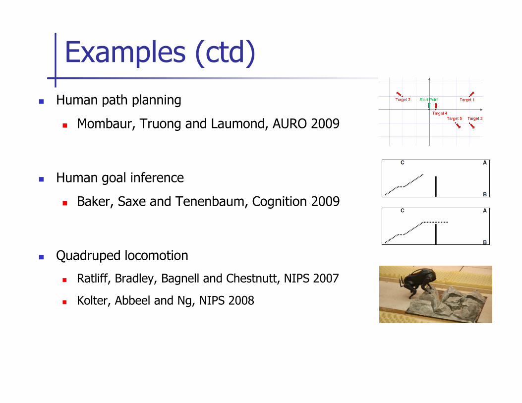
� Human path planning
� Mombaur, Truong and Laumond, AURO 2009
� Human goal inference
� Baker, Saxe and Tenenbaum, Cognition 2009
Examples (ctd)
� Baker, Saxe and Tenenbaum, Cognition 2009
� Quadruped locomotion
� Ratliff, Bradley, Bagnell and Chestnutt, NIPS 2007
� Kolter, Abbeel and Ng, NIPS 2008
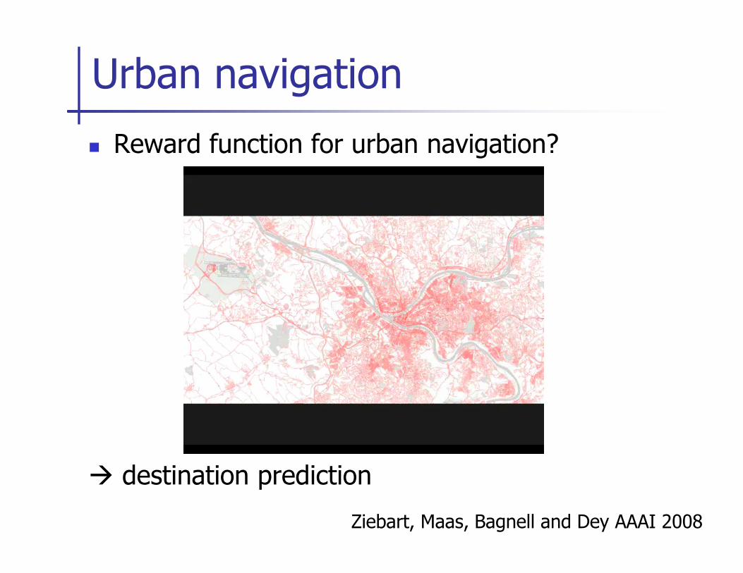
Urban navigation
� Reward function for urban navigation?
Ziebart, Maas, Bagnell and Dey AAAI 2008
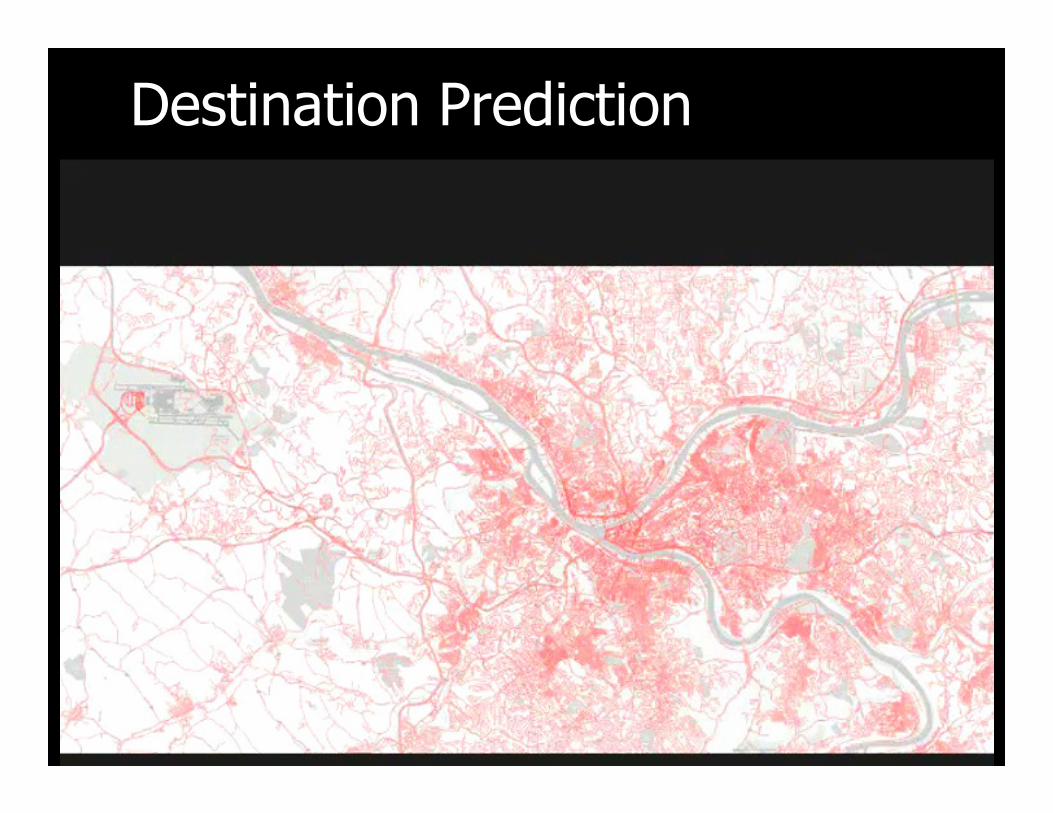
� destination prediction
� Example applications
� Inverse RL vs. behavioral cloning
� Historical sketch of inverse RL
� Mathematical formulations for inverse RL
Lecture outline
� Case studies
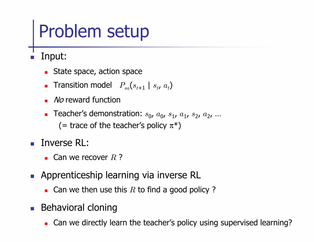
� Input:
� State space, action space
� Transition model Psa(st+1 | st, at)
� No reward function
� Teacher’s demonstration: s0, a0, s1, a1, s2, a2, …
(= trace of the teacher’s policy π*)
Problem setup
(= trace of the teacher’s policy π*)
� Inverse RL:
� Can we recover R ?
� Apprenticeship learning via inverse RL
� Can we then use this R to find a good policy ?
� Behavioral cloning
� Can we directly learn the teacher’s policy using supervised learning?
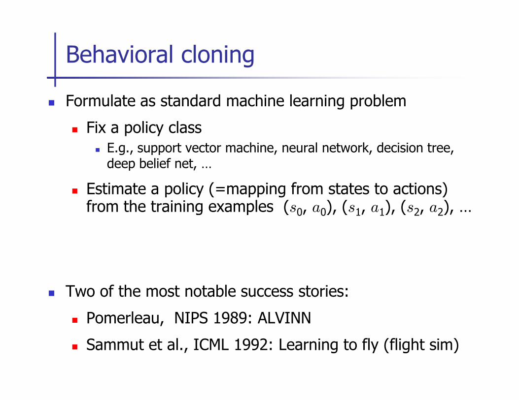
� Formulate as standard machine learning problem
� Fix a policy class
� E.g., support vector machine, neural network, decision tree, deep belief net, …
� Estimate a policy (=mapping from states to actions) from the training examples (s , a ), (s , a ), (s , a ), …
Behavioral cloning
from the training examples (s0, a0), (s1, a1), (s2, a2), …
� Two of the most notable success stories:
� Pomerleau, NIPS 1989: ALVINN
� Sammut et al., ICML 1992: Learning to fly (flight sim)
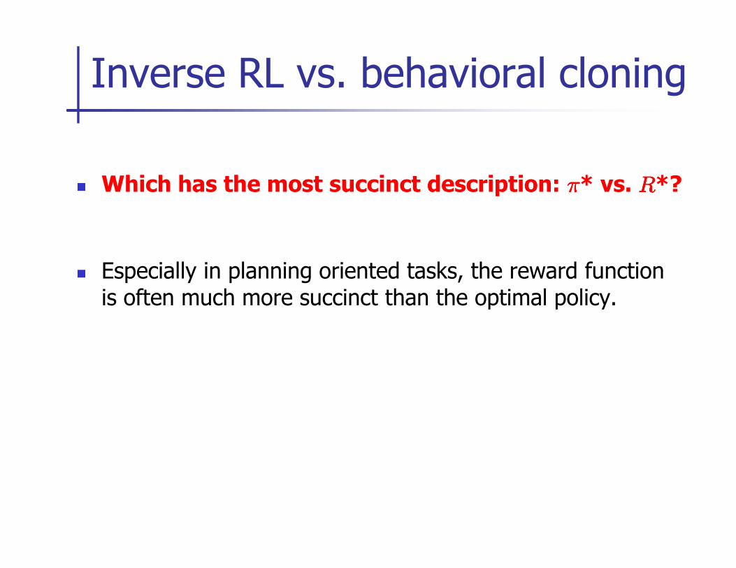
� Which has the most succinct description: ππππ* vs. RRRR*?
� Especially in planning oriented tasks, the reward function is often much more succinct than the optimal policy.
Inverse RL vs. behavioral cloning
is often much more succinct than the optimal policy.

� Example applications
� Inverse RL vs. behavioral cloning
� Historical sketch of inverse RL
� Mathematical formulations for inverse RL
Lecture outline
� Case studies
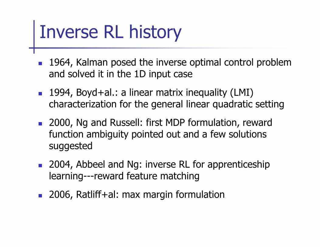
� 1964, Kalman posed the inverse optimal control problem and solved it in the 1D input case
� 1994, Boyd+al.: a linear matrix inequality (LMI) characterization for the general linear quadratic setting
� 2000, Ng and Russell: first MDP formulation, reward
Inverse RL history
� 2000, Ng and Russell: first MDP formulation, reward function ambiguity pointed out and a few solutions suggested
� 2004, Abbeel and Ng: inverse RL for apprenticeship learning---reward feature matching
� 2006, Ratliff+al: max margin formulation
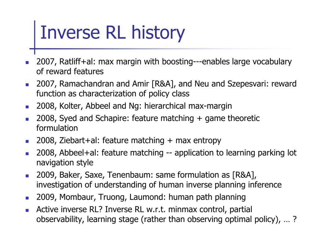
� 2007, Ratliff+al: max margin with boosting---enables large vocabulary of reward features
� 2007, Ramachandran and Amir [R&A], and Neu and Szepesvari: reward function as characterization of policy class
� 2008, Kolter, Abbeel and Ng: hierarchical max-margin
� 2008, Syed and Schapire: feature matching + game theoretic formulation
Inverse RL history
formulation
� 2008, Ziebart+al: feature matching + max entropy
� 2008, Abbeel+al: feature matching -- application to learning parking lot navigation style
� 2009, Baker, Saxe, Tenenbaum: same formulation as [R&A], investigation of understanding of human inverse planning inference
� 2009, Mombaur, Truong, Laumond: human path planning
� Active inverse RL? Inverse RL w.r.t. minmax control, partial observability, learning stage (rather than observing optimal policy), … ?

� Example applications
� Inverse RL vs. behavioral cloning
� Historical sketch of inverse RL
� Mathematical formulations for inverse RL
Lecture outline
� Case studies
Three broad categories of formalizations
� Max margin
� Feature expectation matching
� Interpret reward function as parameterization of a policy class
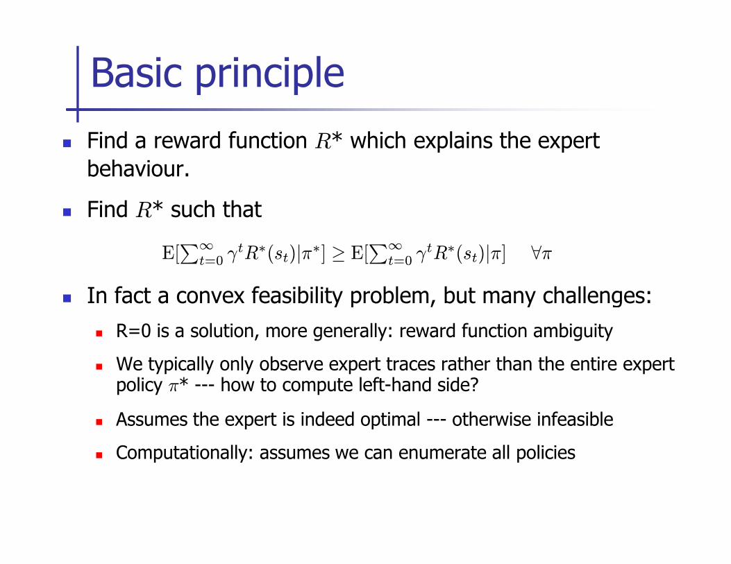
� Find a reward function R* which explains the expert
behaviour.
� Find R* such that
In fact a convex feasibility problem, but many challenges:
Basic principle
E[∑∞
t=0 γtR∗(st)|π∗] ≥ E[
∑∞t=0 γtR∗(st)|π] ∀π
� In fact a convex feasibility problem, but many challenges:
� R=0 is a solution, more generally: reward function ambiguity
� We typically only observe expert traces rather than the entire expert policy π* --- how to compute left-hand side?
� Assumes the expert is indeed optimal --- otherwise infeasible
� Computationally: assumes we can enumerate all policies
� ff
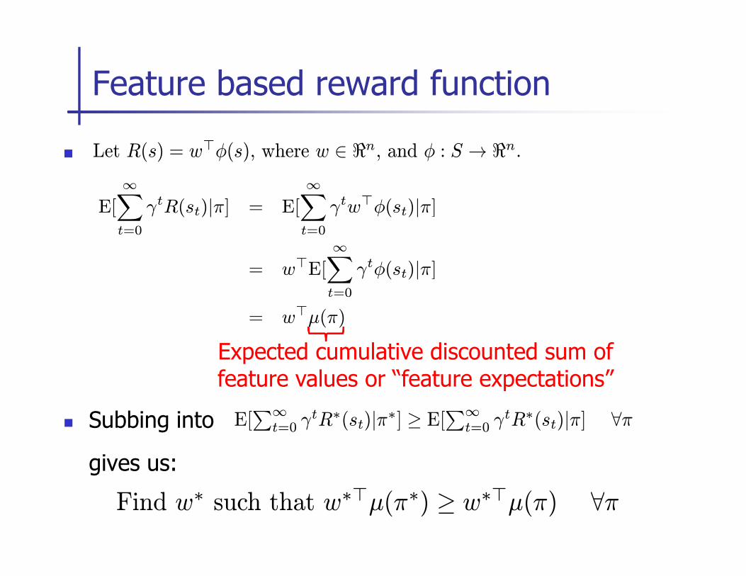
Feature based reward function
Let R(s) = w⊤φ(s), where w ∈ ℜn, and φ : S → ℜn.
E[
∞∑
t=0
γtR(st)|π] = E[
∞∑
t=0
γtw⊤φ(st)|π]
= w⊤E[∞∑
t=0
γtφ(st)|π]
� Subbing into
gives us:
∑
t=0
|
= w⊤µ(π)
Expected cumulative discounted sum of feature values or “feature expectations”
E[∑∞
t=0 γtR∗(st)|π∗] ≥ E[
∑∞t=0 γtR∗(st)|π] ∀π
Find w∗ such that w∗⊤µ(π∗) ≥ w∗⊤µ(π) ∀π
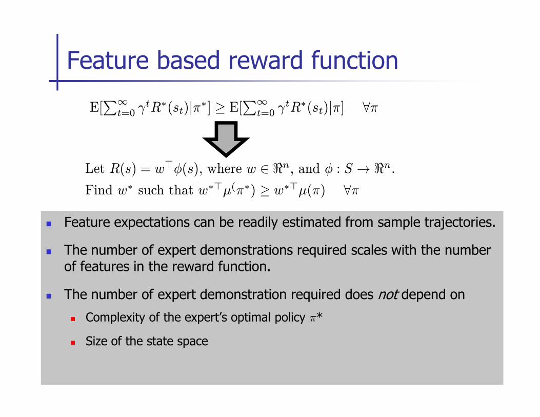
Feature based reward function
Let R(s) = w⊤φ(s), where w ∈ ℜn, and φ : S → ℜn.
Find w∗ such that w∗⊤µ(π∗) ≥ w∗⊤µ(π) ∀π
E[∑∞
t=0 γtR∗(st)|π∗] ≥ E[
∑∞t=0 γtR∗(st)|π] ∀π
� Feature expectations can be readily estimated from sample trajectories.
� The number of expert demonstrations required scales with the number of features in the reward function.
� The number of expert demonstration required does not depend on
� Complexity of the expert’s optimal policy π*
� Size of the state space
� Challenges:
Assumes we know the entire expert policy π* �
Recap of challenges
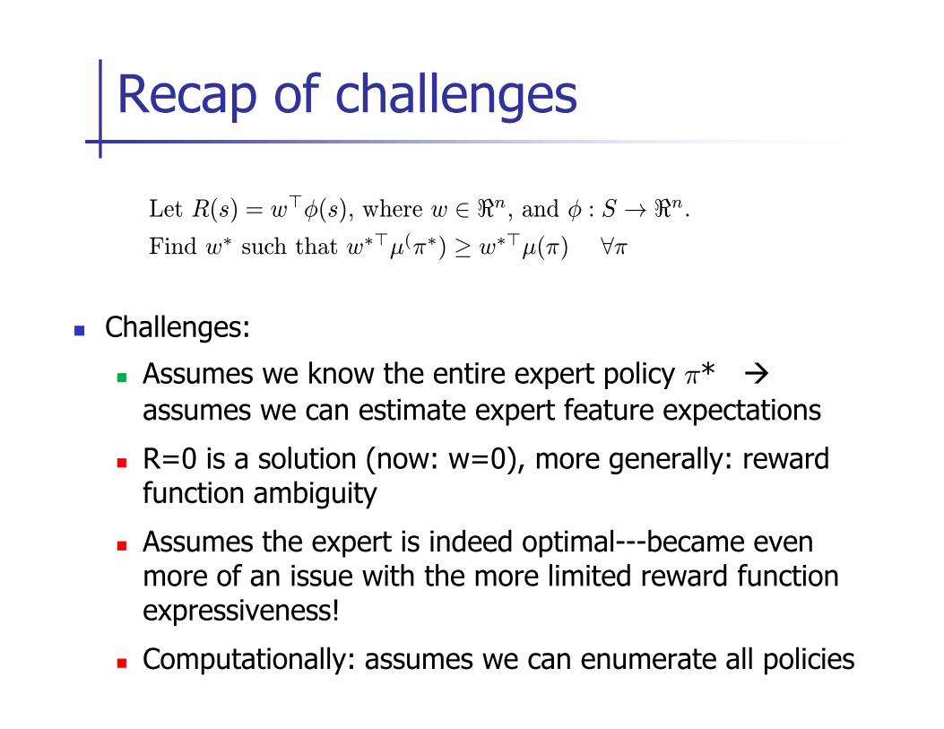
Let R(s) = w⊤φ(s), where w ∈ ℜn, and φ : S → ℜn.
Find w∗ such that w∗⊤µ(π∗) ≥ w∗⊤µ(π) ∀π
� Assumes we know the entire expert policy π* �
assumes we can estimate expert feature expectations
� R=0 is a solution (now: w=0), more generally: reward function ambiguity
� Assumes the expert is indeed optimal---became even more of an issue with the more limited reward function expressiveness!
� Computationally: assumes we can enumerate all policies
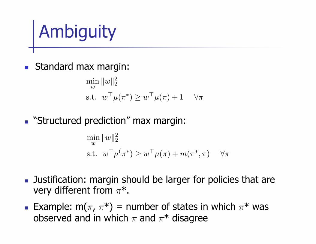
� Standard max margin:
� “Structured prediction” max margin:
Ambiguity
minw‖w‖22
s.t. w⊤µ(π∗) ≥ w⊤µ(π) + 1 ∀π
� “Structured prediction” max margin:
� Justification: margin should be larger for policies that are very different from π*.
� Example: m(π, π*) = number of states in which π* was observed and in which π and π* disagree
minw‖w‖22
s.t. w⊤µ(π∗) ≥ w⊤µ(π) + m(π∗, π) ∀π
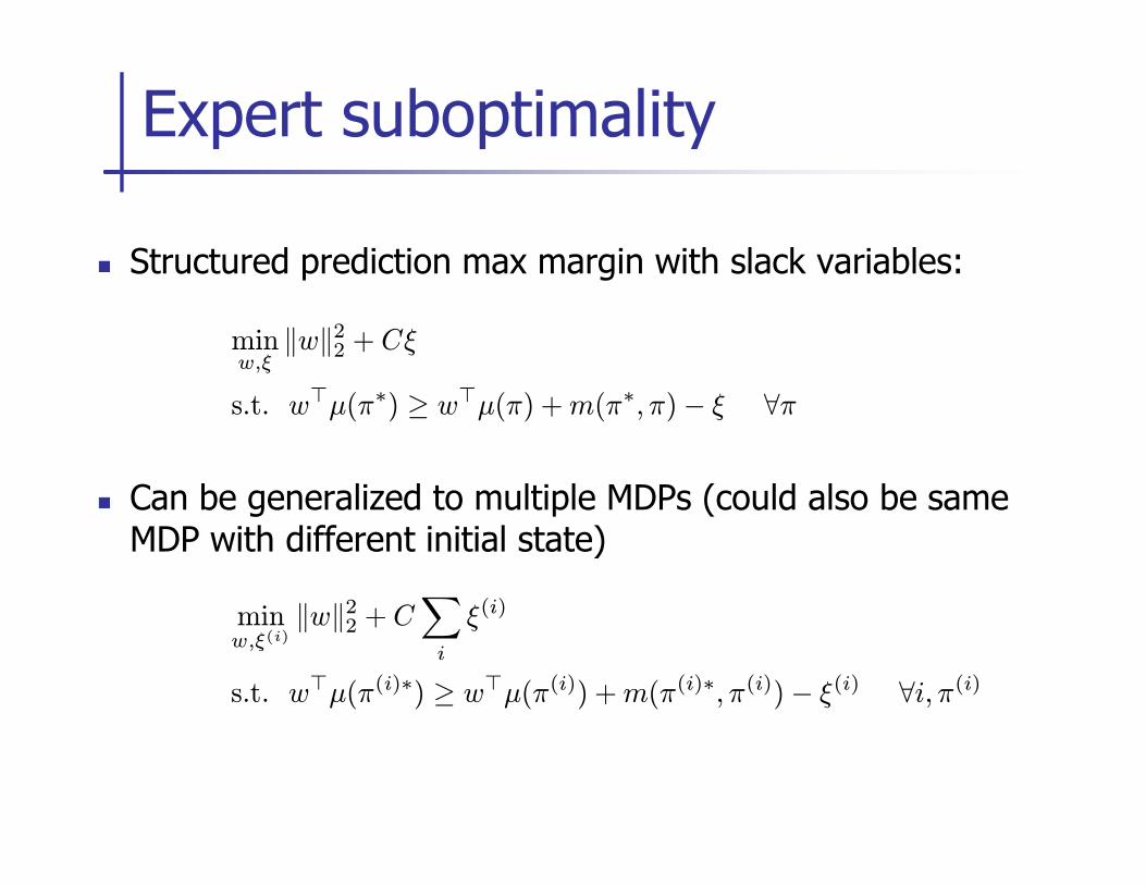
� Structured prediction max margin with slack variables:
Expert suboptimality
minw,ξ
‖w‖22 + Cξ
s.t. w⊤µ(π∗) ≥ w⊤µ(π) + m(π∗, π)− ξ ∀π
� Can be generalized to multiple MDPs (could also be same MDP with different initial state)
minw,ξ(i)
‖w‖22 + C∑
i
ξ(i)
s.t. w⊤µ(π(i)∗) ≥ w⊤µ(π(i)) + m(π(i)∗, π(i))− ξ(i) ∀i, π(i)

Complete max-margin formulation
[Ratliff, Zinkevich and Bagnell, 2006]
minw‖w‖22 + C
∑
i
ξ(i)
s.t. w⊤µ(π(i)∗) ≥ w⊤µ(π(i)) + m(π(i)∗, π(i))− ξ(i) ∀i, π(i)
� Resolved: access to π*, ambiguity, expert suboptimality
� One challenge remains: very large number of constraints
� Ratliff+al use subgradient methods.
� In this lecture: constraint generation
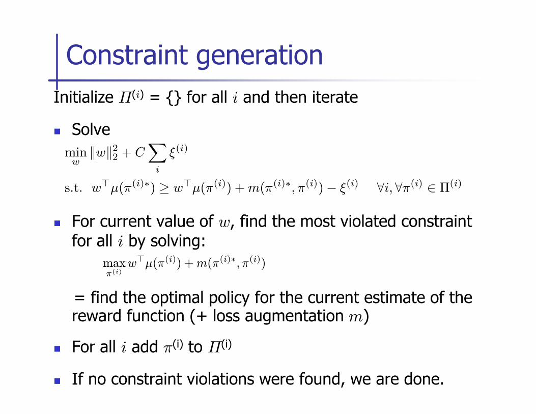
Initialize Π(i) = {} for all i and then iterate
� Solve
Constraint generation
minw‖w‖22 + C
∑
i
ξ(i)
s.t. w⊤µ(π(i)∗) ≥ w⊤µ(π(i)) + m(π(i)∗, π(i))− ξ(i) ∀i, ∀π(i) ∈ Π(i)
� For current value of w, find the most violated constraint for all i by solving:
= find the optimal policy for the current estimate of the reward function (+ loss augmentation m)
� For all i add π(i) to Π(i)
� If no constraint violations were found, we are done.
maxπ(i)
w⊤µ(π(i)) + m(π(i)∗, π(i))
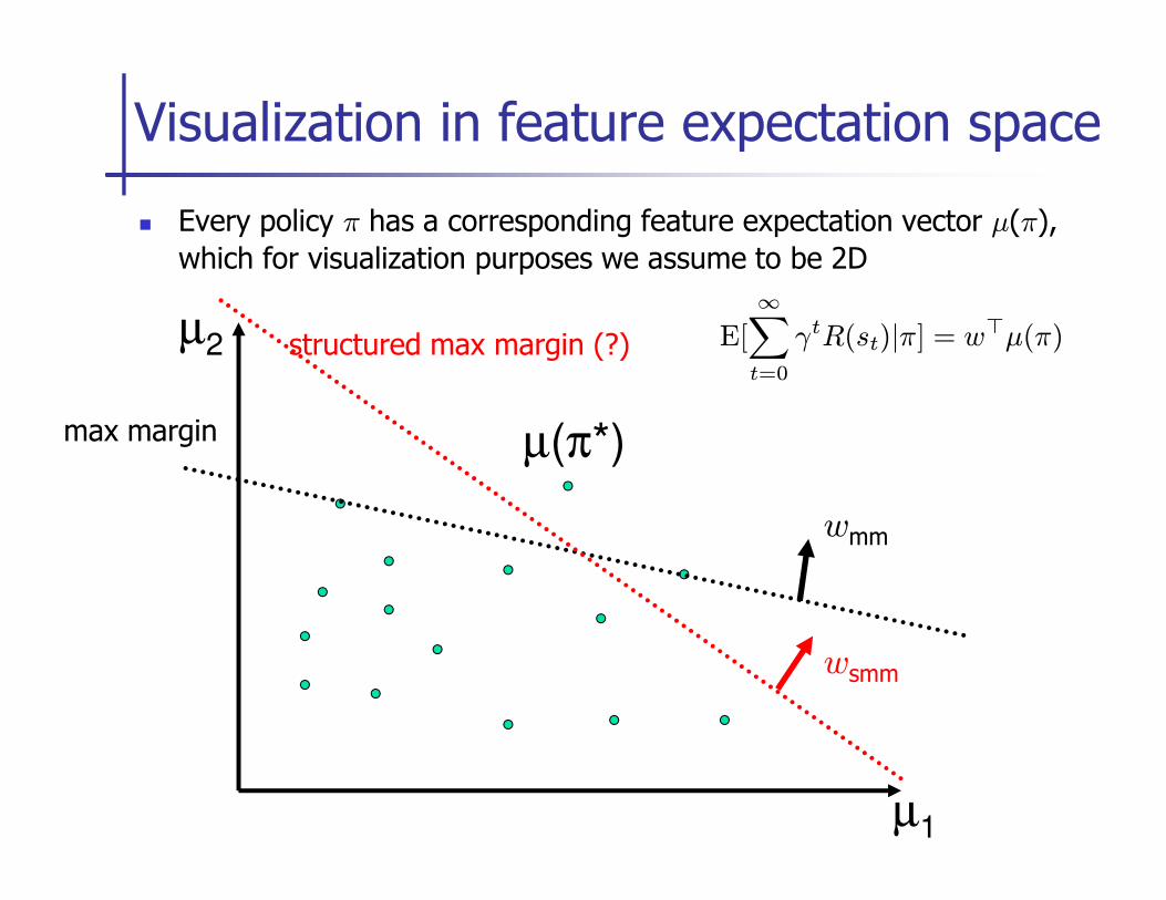
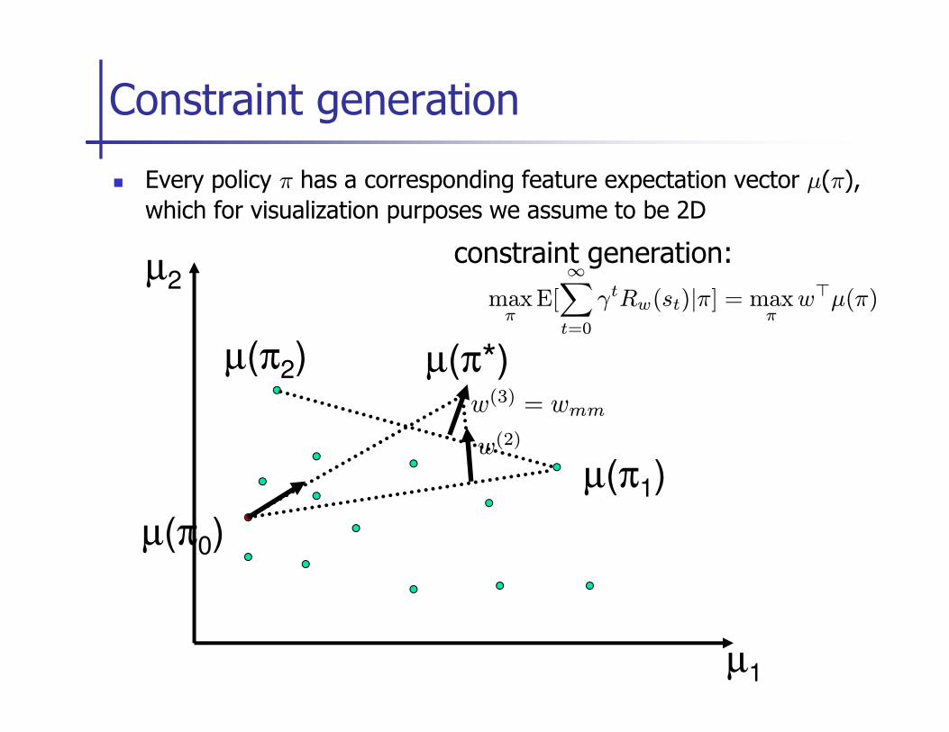
� Every policy π has a corresponding feature expectation vector µ(π),
which for visualization purposes we assume to be 2D
Visualization in feature expectation space
µ2
µ(π*)
E[
∞∑
t=0
γtR(st)|π] = w⊤µ(π)
max margin
structured max margin (?)
µ1
µ(π*)
wmm
wsmm
� Every policy π has a corresponding feature expectation vector µ(π),
which for visualization purposes we assume to be 2D
Constraint generation
µ(π2)
µ2
µ(π*)
maxπ
E[
∞∑
t=0
γtRw(st)|π] = maxπ
w⊤µ(π)
constraint generation:
µ1
µ(π0)
µ(π2) µ(π*)
µ(π1)w(2)
w(3) = wmm
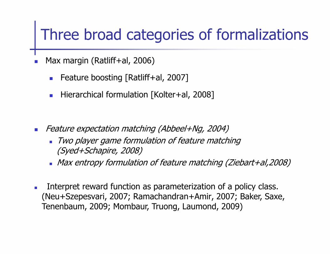
Three broad categories of formalizations
� Max margin (Ratliff+al, 2006)
� Feature boosting [Ratliff+al, 2007]
� Hierarchical formulation [Kolter+al, 2008]
� Feature expectation matching (Abbeel+Ng, 2004)� Feature expectation matching (Abbeel+Ng, 2004)
� Two player game formulation of feature matching (Syed+Schapire, 2008)
� Max entropy formulation of feature matching (Ziebart+al,2008)
� Interpret reward function as parameterization of a policy class. (Neu+Szepesvari, 2007; Ramachandran+Amir, 2007; Baker, Saxe, Tenenbaum, 2009; Mombaur, Truong, Laumond, 2009)
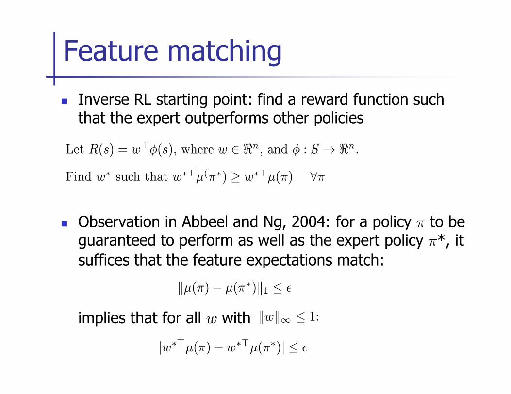
� Inverse RL starting point: find a reward function such that the expert outperforms other policies
Feature matching
Let R(s) = w⊤φ(s), where w ∈ ℜn, and φ : S → ℜn.
Find w∗ such that w∗⊤µ(π∗) ≥ w∗⊤µ(π) ∀π
� Observation in Abbeel and Ng, 2004: for a policy π to be guaranteed to perform as well as the expert policy π*, it
suffices that the feature expectations match:
implies that for all w with
‖µ(π)− µ(π∗)‖1 ≤ ǫ
‖w‖∞ ≤ 1:
|w∗⊤µ(π)− w∗⊤µ(π∗)| ≤ ǫ
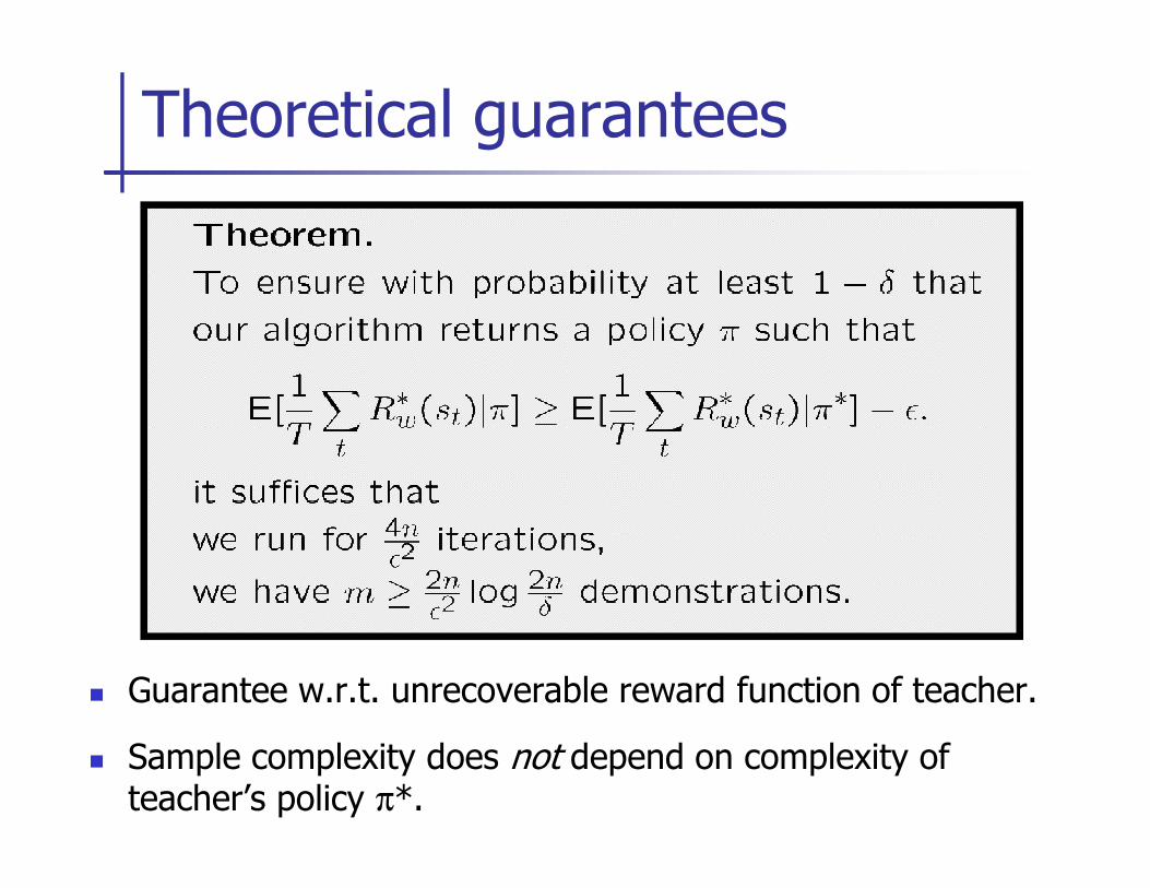
Theoretical guarantees
� Guarantee w.r.t. unrecoverable reward function of teacher.
� Sample complexity does not depend on complexity of teacher’s policy π*.
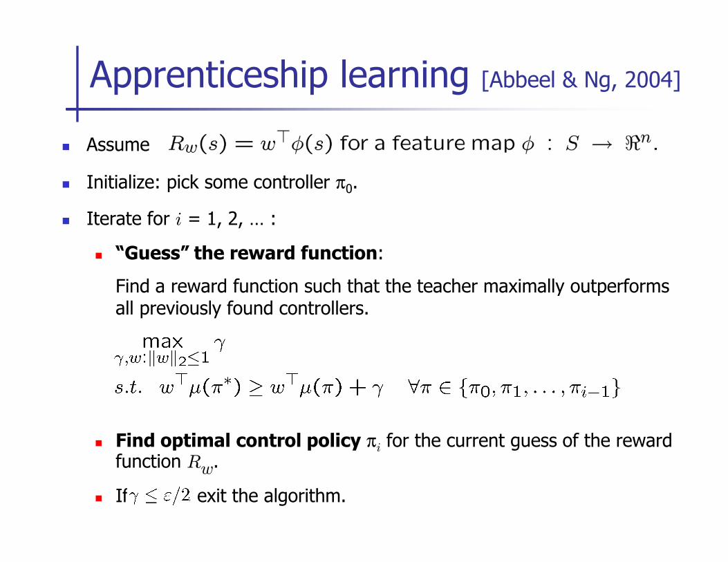
Apprenticeship learning [Abbeel & Ng, 2004]
� Assume
� Initialize: pick some controller π0.
� Iterate for i = 1, 2, … :
� “Guess” the reward function:
Find a reward function such that the teacher maximally outperforms Find a reward function such that the teacher maximally outperforms all previously found controllers.
� Find optimal control policy πi for the current guess of the reward function Rw.
� If , exit the algorithm.
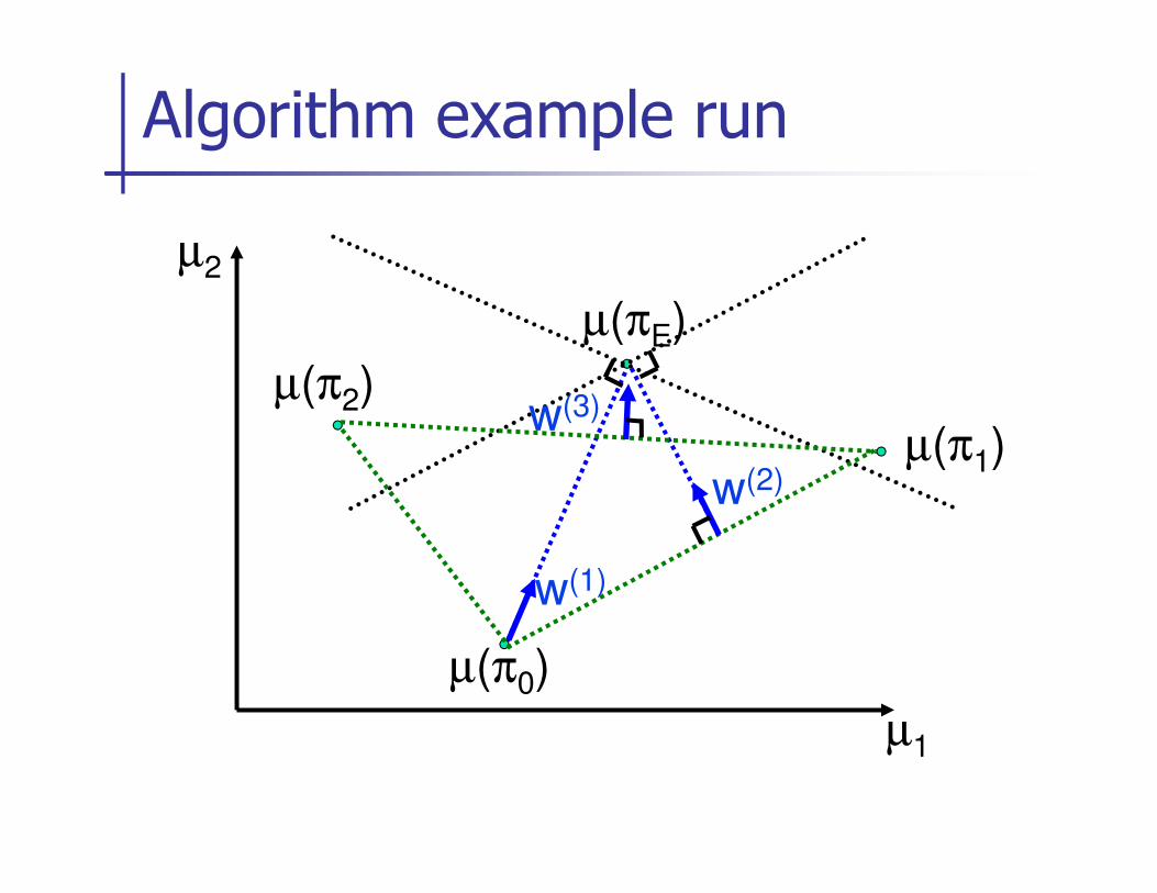
Algorithm example run
µ(π1)
µ(π2)
µ2
w(3)
µ(πE)
µ1
µ(π0)
w(1)
w(2)µ(π1)
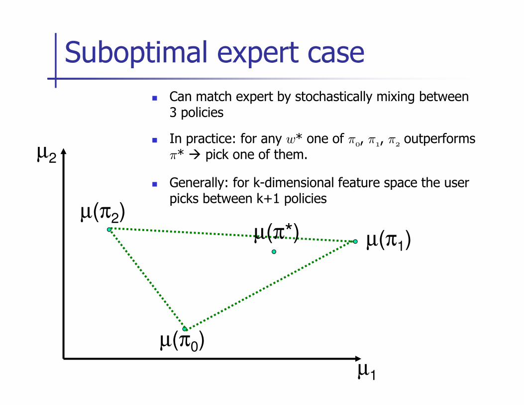
Suboptimal expert case
µ(π )
µ2
� Can match expert by stochastically mixing between 3 policies
� In practice: for any w* one of π, π, π outperforms π* � pick one of them.
� Generally: for k-dimensional feature space the user picks between k+1 policies
µ1
µ(π0)
µ(π1)
µ(π2)µ(π*)
picks between k+1 policies
� If expert suboptimal then the resulting policy is a mixture of somewhat arbitrary policies which have expert in their convex hull.
� In practice: pick the best one of this set and pick the
Feature expectation matching
� In practice: pick the best one of this set and pick the corresponding reward function.
� Next:
� Syed and Schapire, 2008.
� Ziebart+al, 2008.
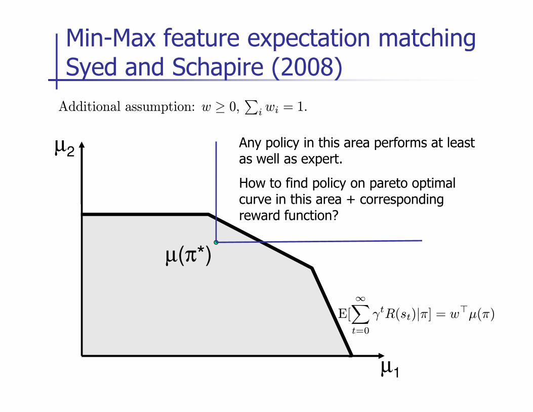
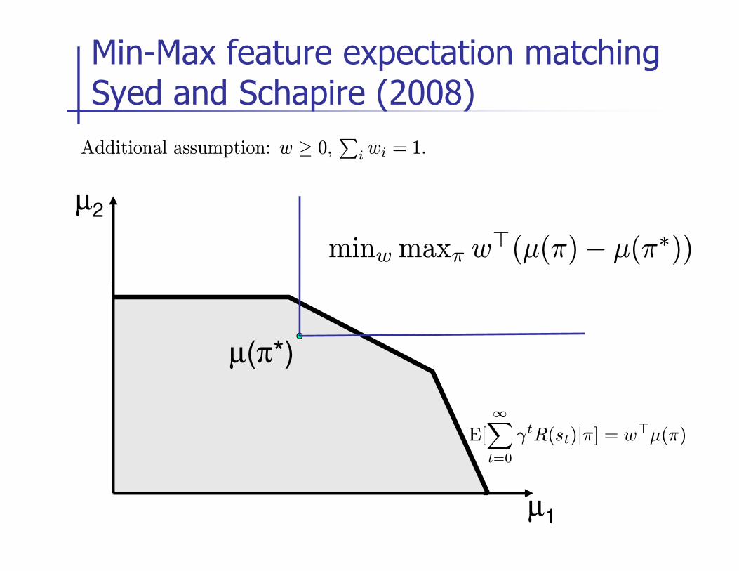
Min-Max feature expectation matching Syed and Schapire (2008)
µ2
Additional assumption: w ≥ 0,∑
i wi = 1.
Any policy in this area performs at least as well as expert.
How to find policy on pareto optimal curve in this area + corresponding
µ1
µ(π*)
E[
∞∑
t=0
γtR(st)|π] = w⊤µ(π)
curve in this area + corresponding reward function?
Min-Max feature expectation matching Syed and Schapire (2008)
µ2
Additional assumption: w ≥ 0,∑
i wi = 1.
minwmaxπ w⊤(µ(π)− µ(π∗))
µ1
µ(π*)
E[
∞∑
t=0
γtR(st)|π] = w⊤µ(π)
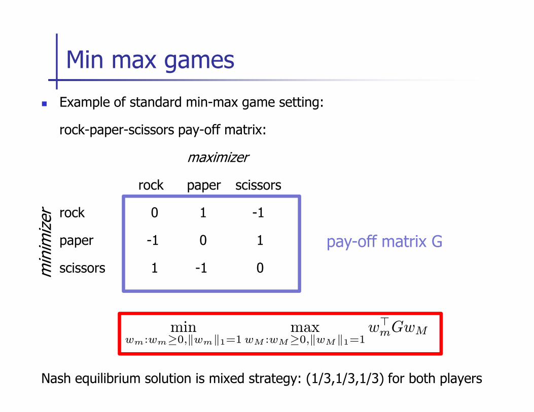
� Example of standard min-max game setting:
rock-paper-scissors pay-off matrix:
maximizer
rock paper scissors
rock 0 1 -1
Min max games
rock 0 1 -1
paper -1 0 1
scissors 1 -1 0
Nash equilibrium solution is mixed strategy: (1/3,1/3,1/3) for both players
min
imiz
er
pay-off matrix G
minwm:wm≥0,‖wm‖1=1
maxwM :wM≥0,‖wM‖1=1
w⊤mGwM
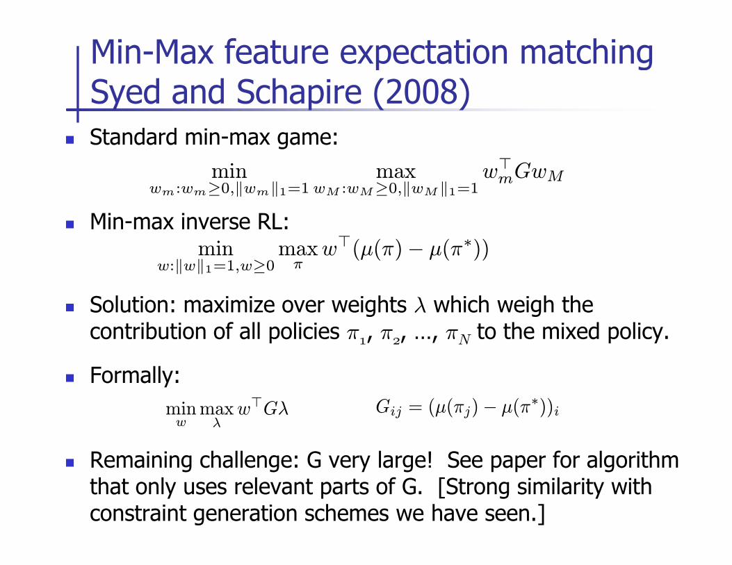
� Standard min-max game:
� Min-max inverse RL:
Min-Max feature expectation matching Syed and Schapire (2008)
minw:‖w‖1=1,w≥0
maxπ
w⊤(µ(π)− µ(π∗))
minwm:wm≥0,‖wm‖1=1
maxwM :wM≥0,‖wM‖1=1
w⊤mGwM
� Solution: maximize over weights λ which weigh the contribution of all policies π, π, …, πN to the mixed policy.
� Formally:
� Remaining challenge: G very large! See paper for algorithm that only uses relevant parts of G. [Strong similarity with constraint generation schemes we have seen.]
minw
maxλ
w⊤Gλ Gij = (µ(πj)− µ(π∗))i
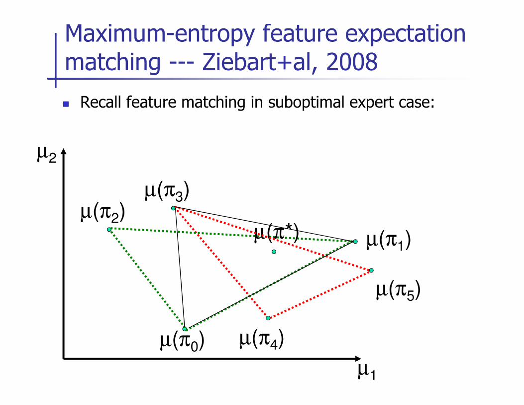
� Recall feature matching in suboptimal expert case:
Maximum-entropy feature expectation matching --- Ziebart+al, 2008
µ(π )
µ2
µ(π3)
µ1
µ(π0)
µ(π1)
µ(π2)µ(π*)
µ(π5)
µ(π4)
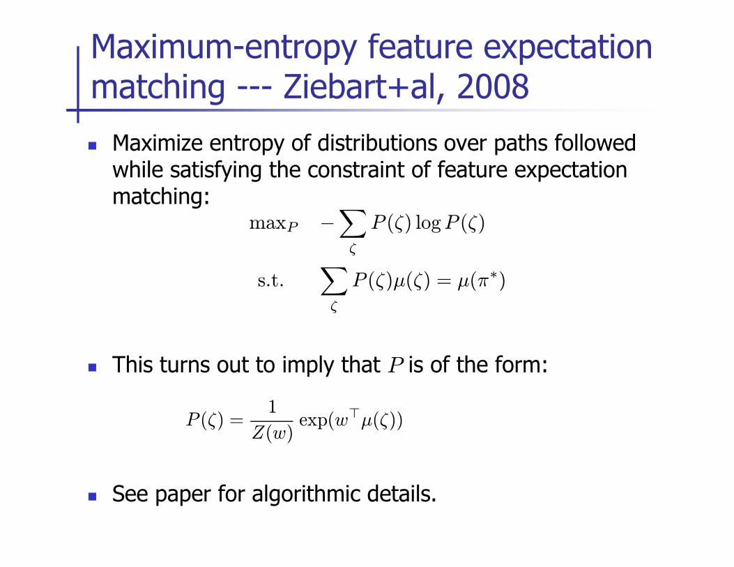
� Maximize entropy of distributions over paths followed while satisfying the constraint of feature expectation matching:
Maximum-entropy feature expectation matching --- Ziebart+al, 2008
maxP −∑
ζ
P (ζ) logP (ζ)
s.t.∑
P (ζ)µ(ζ) = µ(π∗)
� This turns out to imply that P is of the form:
� See paper for algorithmic details.
s.t.∑
ζ
P (ζ)µ(ζ) = µ(π∗)
P (ζ) =1
Z(w)exp(w⊤µ(ζ))
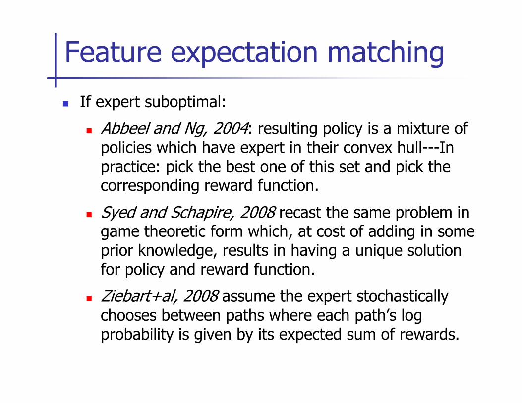
� If expert suboptimal:
� Abbeel and Ng, 2004: resulting policy is a mixture of policies which have expert in their convex hull---In practice: pick the best one of this set and pick the corresponding reward function.
Feature expectation matching
� Syed and Schapire, 2008 recast the same problem in game theoretic form which, at cost of adding in some prior knowledge, results in having a unique solution for policy and reward function.
� Ziebart+al, 2008 assume the expert stochastically chooses between paths where each path’s log probability is given by its expected sum of rewards.
� Example applications
� Inverse RL vs. behavioral cloning
� Historical sketch of inverse RL
� Mathematical formulations for inverse RL
Max-margin
Lecture outline
� Max-margin
� Feature matching
� Reward function parameterizing the policy class
� Case studies
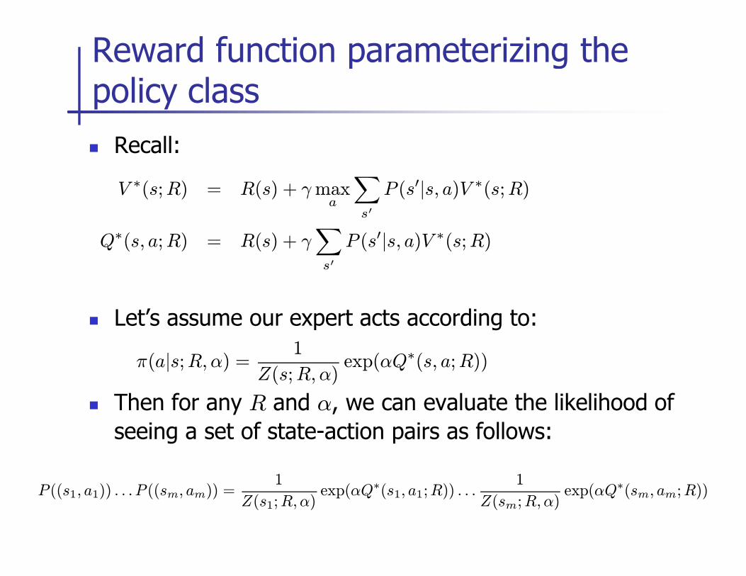
� Recall:
Reward function parameterizing the policy class
V ∗(s;R) = R(s) + γ maxa
∑
s′
P (s′|s, a)V ∗(s;R)
Q∗(s, a;R) = R(s) + γ∑
s′
P (s′|s, a)V ∗(s;R)
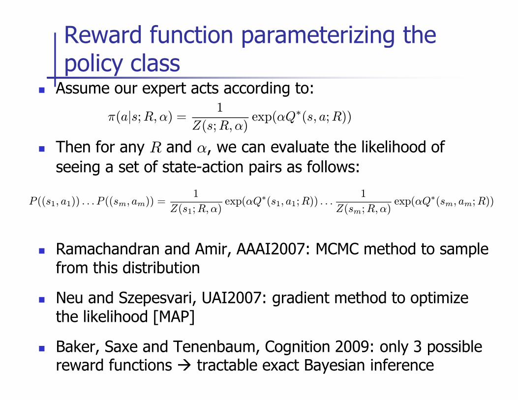
� Let’s assume our expert acts according to:
� Then for any R and α, we can evaluate the likelihood of
seeing a set of state-action pairs as follows:
π(a|s;R, α) =1
Z(s;R, α)exp(αQ∗(s, a;R))
P ((s1, a1)) . . . P ((sm, am)) =1
Z(s1;R, α)exp(αQ∗(s1, a1;R)) . . .
1
Z(sm;R, α)exp(αQ∗(sm, am;R))
� Assume our expert acts according to:
� Then for any R and α, we can evaluate the likelihood of
seeing a set of state-action pairs as follows:
Reward function parameterizing the policy class
π(a|s;R, α) =1
Z(s;R, α)exp(αQ∗(s, a;R))
P ((s , a )) . . . P ((s , a )) =1
exp(αQ∗(s , a ;R)) . . .1
exp(αQ∗(s , a ;R))
� Ramachandran and Amir, AAAI2007: MCMC method to sample from this distribution
� Neu and Szepesvari, UAI2007: gradient method to optimize the likelihood [MAP]
� Baker, Saxe and Tenenbaum, Cognition 2009: only 3 possible reward functions � tractable exact Bayesian inference
P ((s1, a1)) . . . P ((sm, am)) =Z(s1;R, α)
exp(αQ∗(s1, a1;R)) . . .Z(sm;R, α)
exp(αQ∗(sm, am;R))
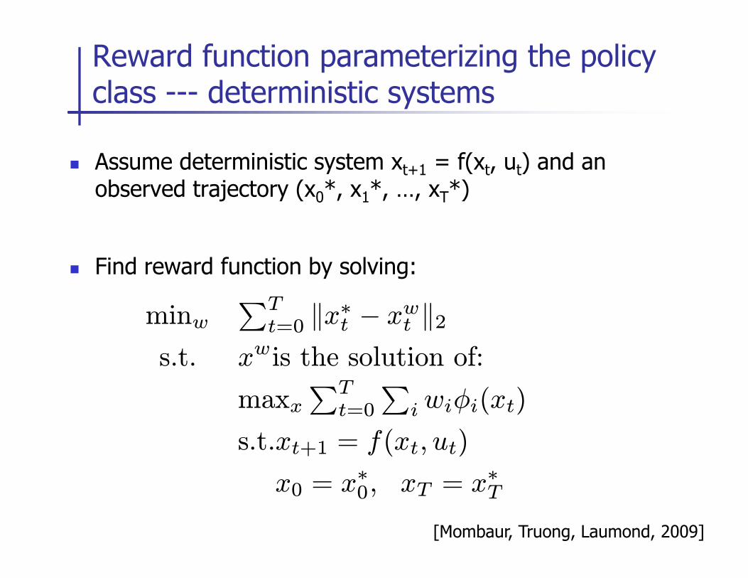
� Assume deterministic system xt+1 = f(xt, ut) and an observed trajectory (x0*, x1*, …, xT*)
� Find reward function by solving:
Reward function parameterizing the policy class --- deterministic systems
minw∑T
t=0 ‖x∗t − xwt ‖2
s.t. xwis the solution of:
maxx∑T
t=0
∑i wiφi(xt)
s.t.xt+1 = f(xt, ut)
x0 = x∗0, xT = x∗T
[Mombaur, Truong, Laumond, 2009]
� Example applications
� Inverse RL vs. behavioral cloning
� History of inverse RL
� Mathematical formulations for inverse RL
Lecture outline
� Case studies: (1) Highway driving, (2) Crusher, (3) Parking lot navigation, (4) Route inference, (5) Human path planning, (6) Human inverse planning, (7) Quadruped locomotion
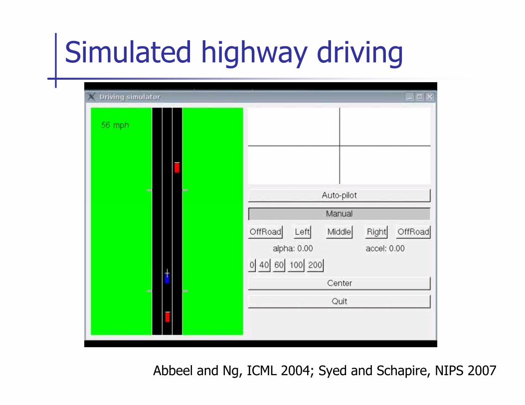
Simulated highway driving
Abbeel and Ng, ICML 2004; Syed and Schapire, NIPS 2007
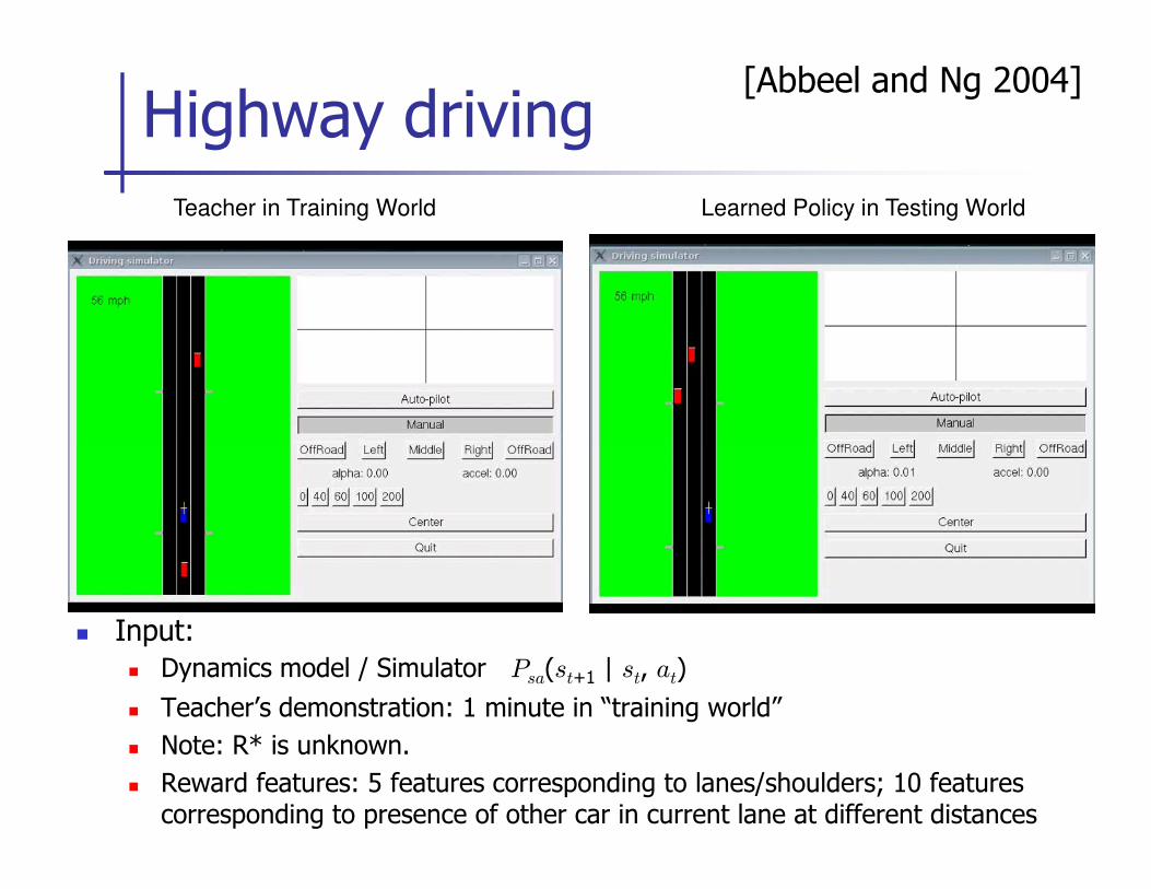
Highway driving
Teacher in Training World Learned Policy in Testing World
[Abbeel and Ng 2004]
� Input:
� Dynamics model / Simulator Psa(st+1 | st, at)
� Teacher’s demonstration: 1 minute in “training world”
� Note: R* is unknown.
� Reward features: 5 features corresponding to lanes/shoulders; 10 features corresponding to presence of other car in current lane at different distances
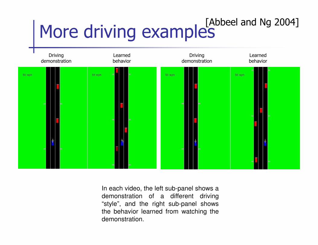
More driving examplesDriving
demonstrationDriving
demonstrationLearned behavior
Learned behavior
[Abbeel and Ng 2004]
In each video, the left sub-panel shows a
demonstration of a different driving
“style”, and the right sub-panel shows
the behavior learned from watching the
demonstration.

Crusher
RSS 2008: Dave Silver and Drew Bagnell
Learning movie
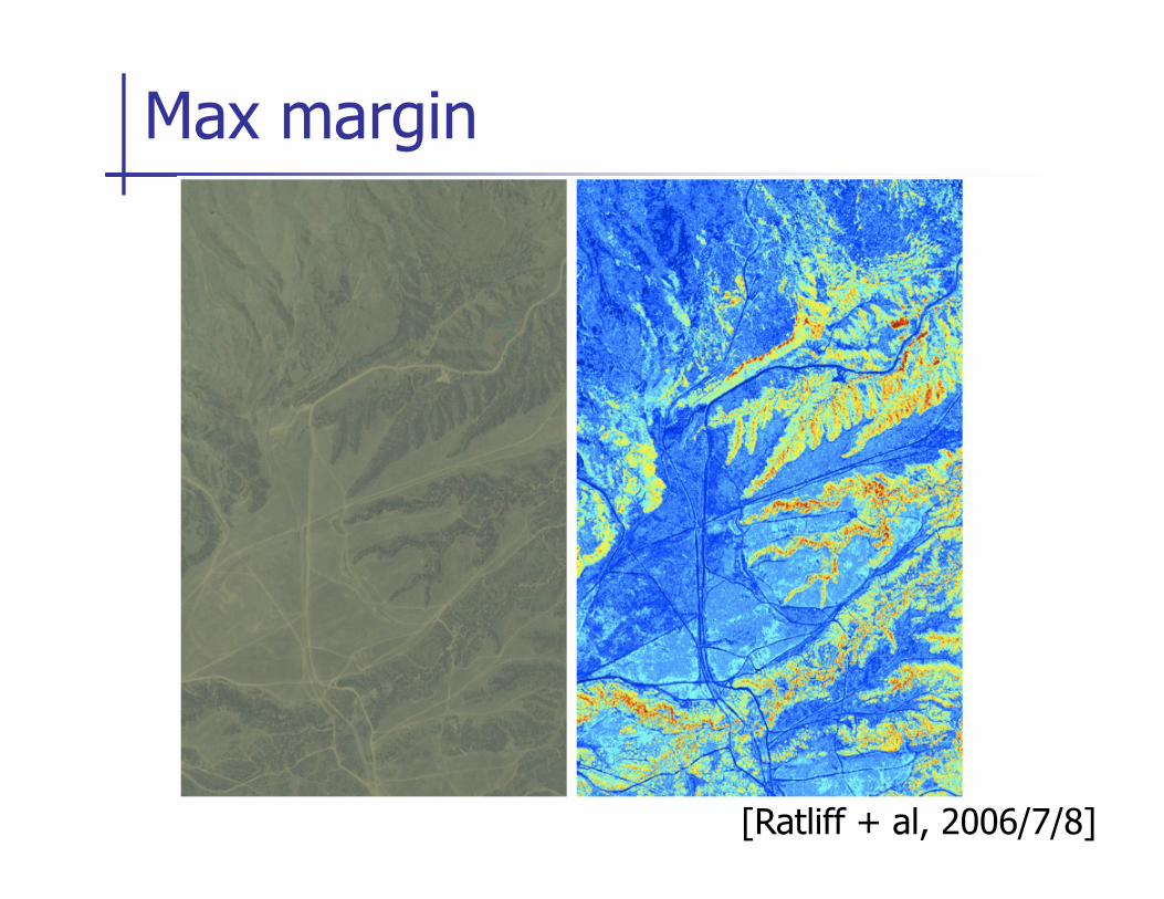
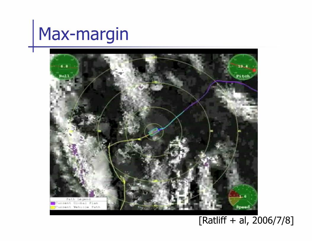
Max margin
[Ratliff + al, 2006/7/8]
Max-margin
[Ratliff + al, 2006/7/8]
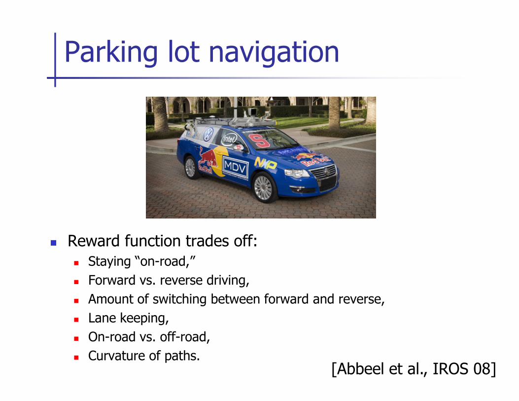
Parking lot navigation
[Abbeel et al., IROS 08]
� Reward function trades off:
� Staying “on-road,”
� Forward vs. reverse driving,
� Amount of switching between forward and reverse,
� Lane keeping,
� On-road vs. off-road,
� Curvature of paths.
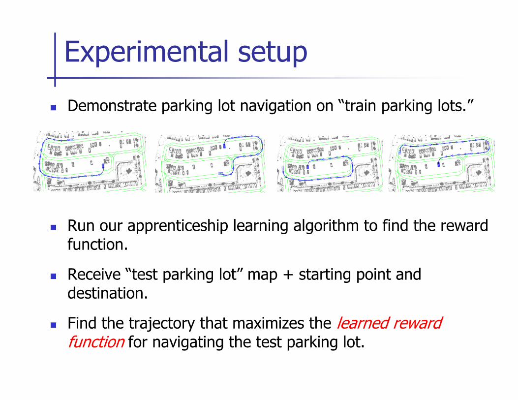
� Demonstrate parking lot navigation on “train parking lots.”
Experimental setup
� Run our apprenticeship learning algorithm to find the reward function.
� Receive “test parking lot” map + starting point and destination.
� Find the trajectory that maximizes the learned reward function for navigating the test parking lot.
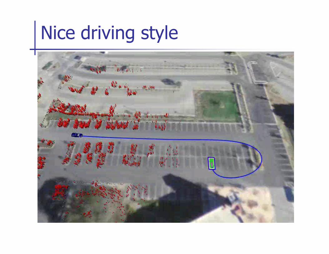
Nice driving style
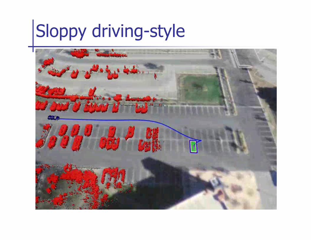
Sloppy driving-style
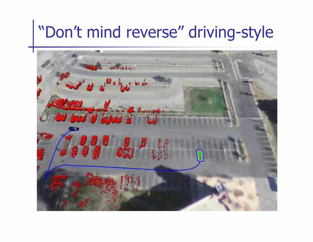
“Don’t mind reverse” driving-style
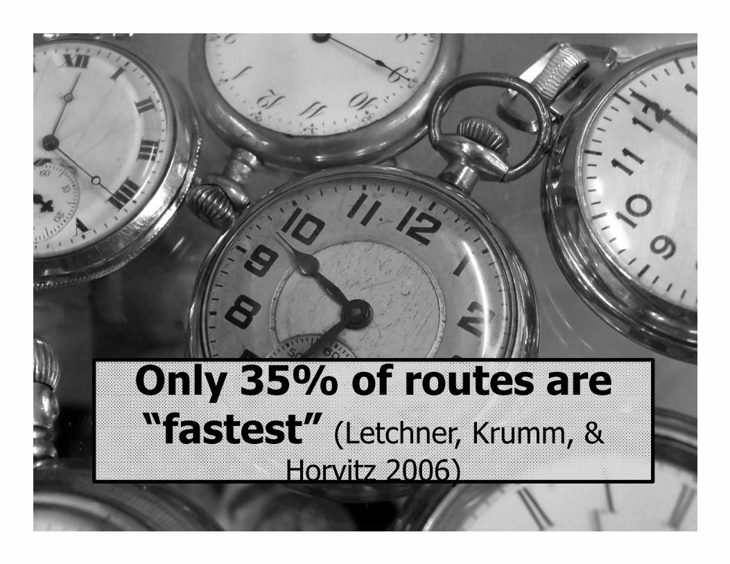
Only 35% of routes are “fastest” (Letchner, Krumm, &
Horvitz 2006)
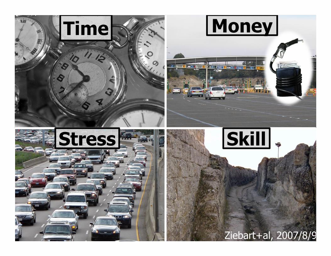
Time Money
Stress SkillStress Skill
Ziebart+al, 2007/8/9
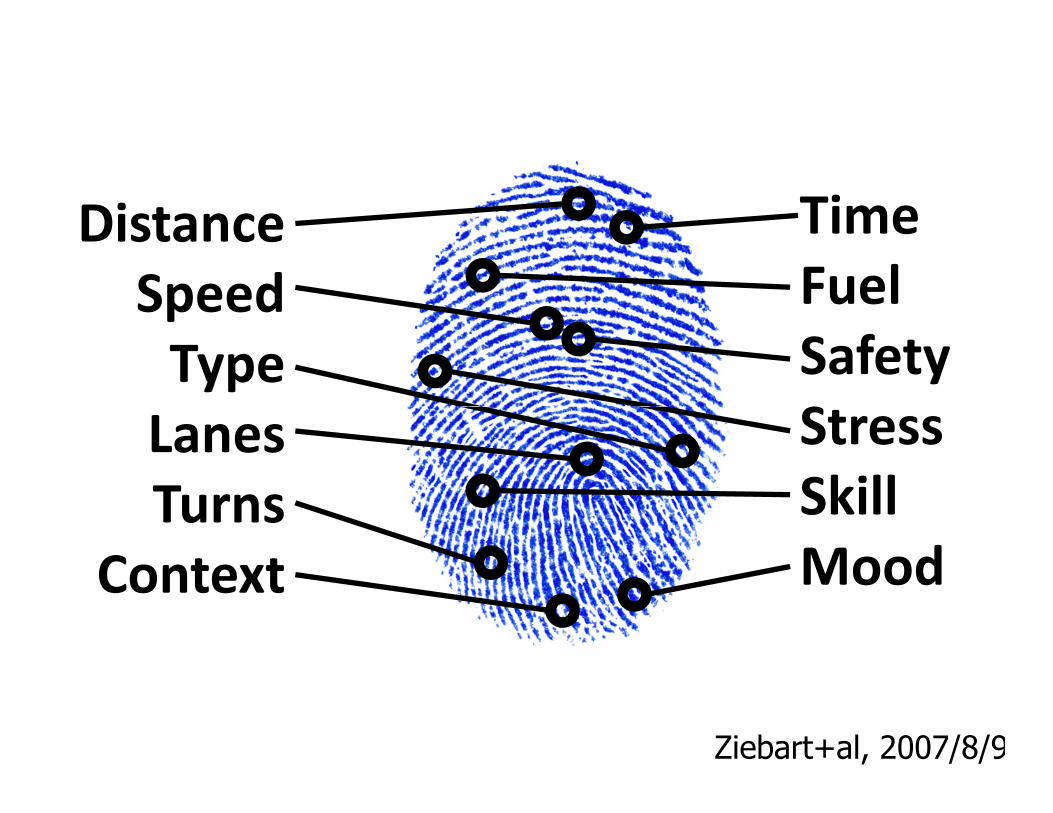
Time
Fuel
Safety
Stress
Distance
Speed
Type
Lanes Stress
Skill
Mood
Lanes
Turns
Context
Ziebart+al, 2007/8/9
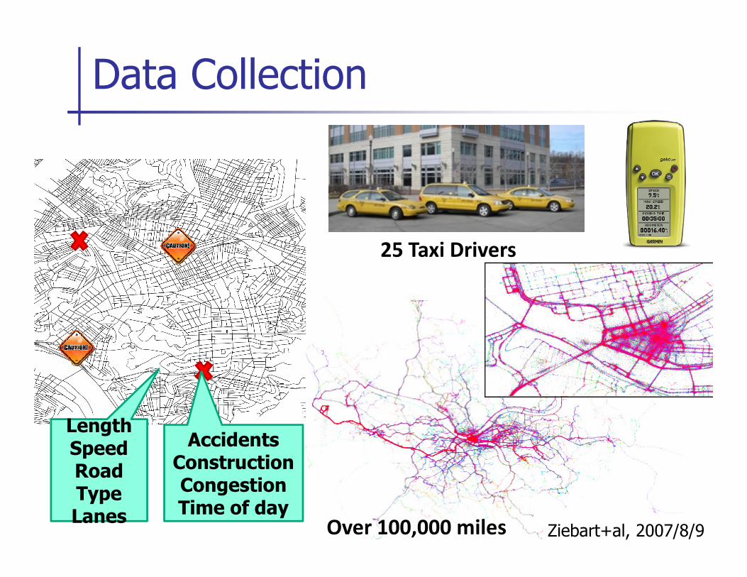
Data Collection
25 Taxi Drivers
LengthSpeedRoad TypeLanes
AccidentsConstructionCongestionTime of day
Over 100,000 miles Ziebart+al, 2007/8/9
Destination Prediction
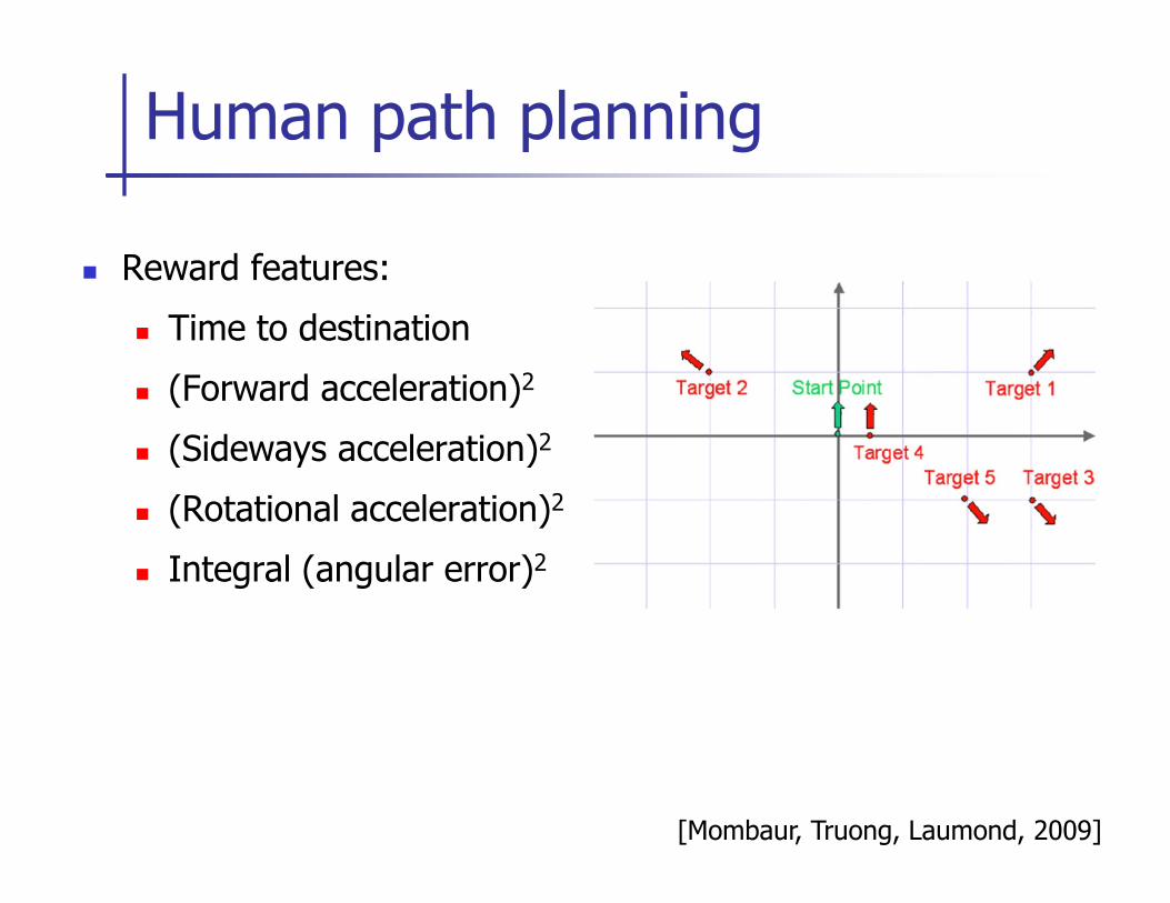
� Reward features:
� Time to destination
� (Forward acceleration)2
� (Sideways acceleration)2
Human path planning
� (Sideways acceleration)2
� (Rotational acceleration)2
� Integral (angular error)2
[Mombaur, Truong, Laumond, 2009]
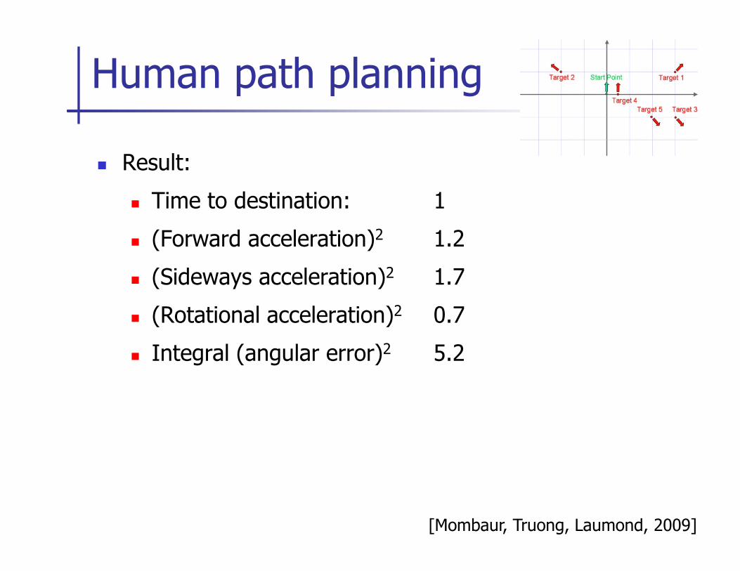
� Result:
� Time to destination: 1
� (Forward acceleration)2 1.2
� (Sideways acceleration)2 1.7
Human path planning
� (Sideways acceleration) 1.7
� (Rotational acceleration)2 0.7
� Integral (angular error)2 5.2
[Mombaur, Truong, Laumond, 2009]
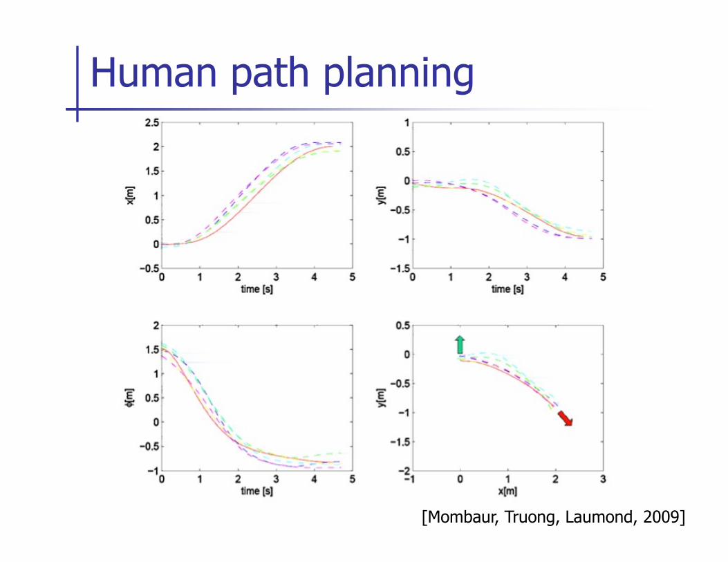
Human path planning
[Mombaur, Truong, Laumond, 2009]
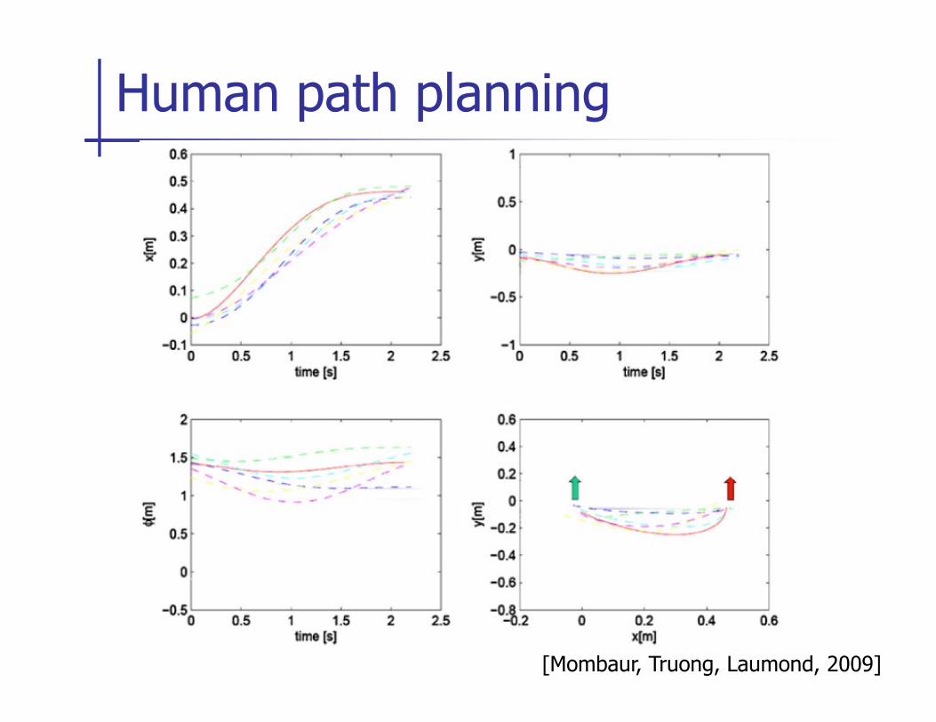
Human path planning
[Mombaur, Truong, Laumond, 2009]
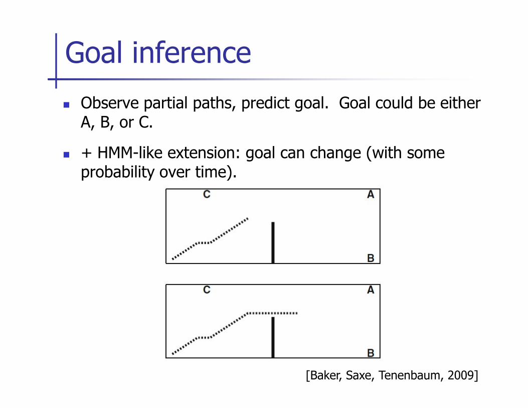
� Observe partial paths, predict goal. Goal could be either A, B, or C.
� + HMM-like extension: goal can change (with some probability over time).
Goal inference
[Baker, Saxe, Tenenbaum, 2009]
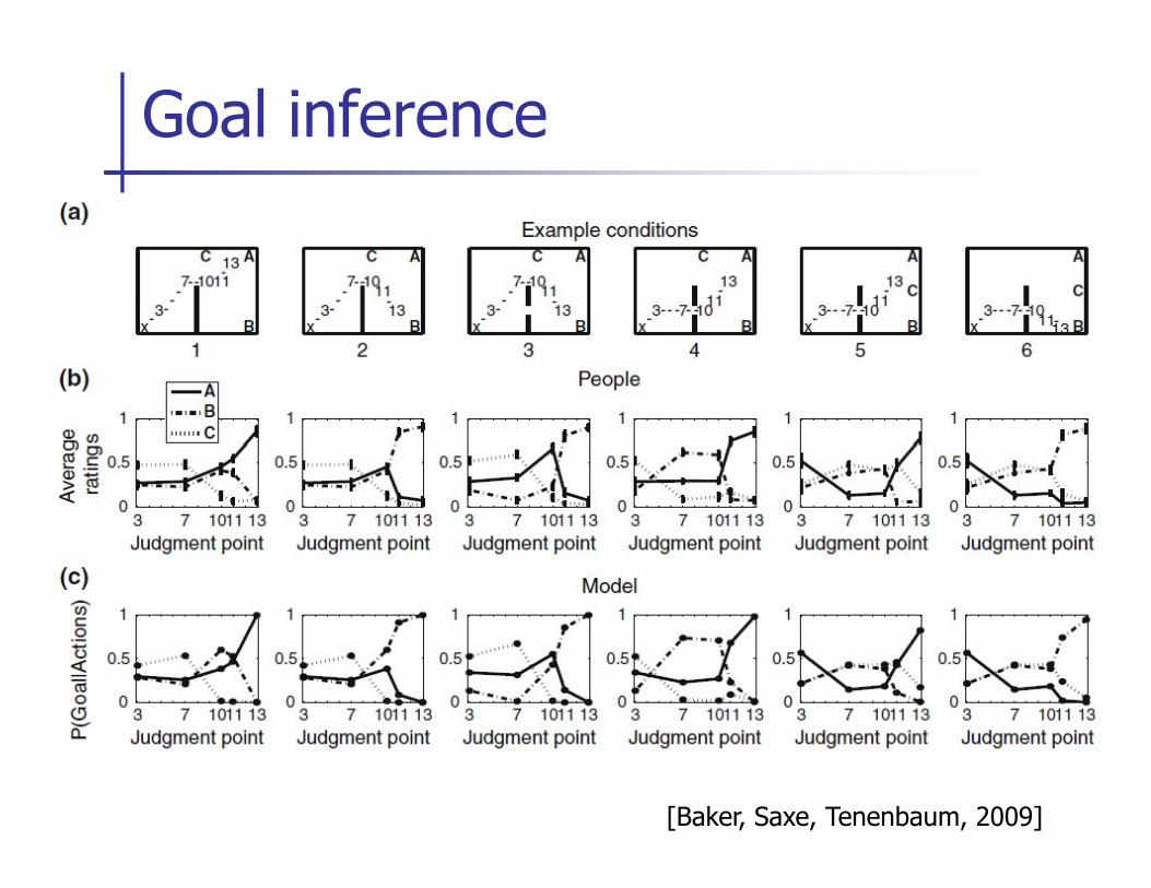
� Observe partial paths, predict goal. Goal could be either A, B, or C.
Goal inference
[Baker, Saxe, Tenenbaum, 2009]
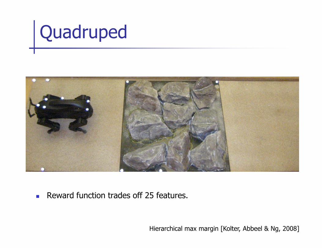
Quadruped
� Reward function trades off 25 features.
Hierarchical max margin [Kolter, Abbeel & Ng, 2008]
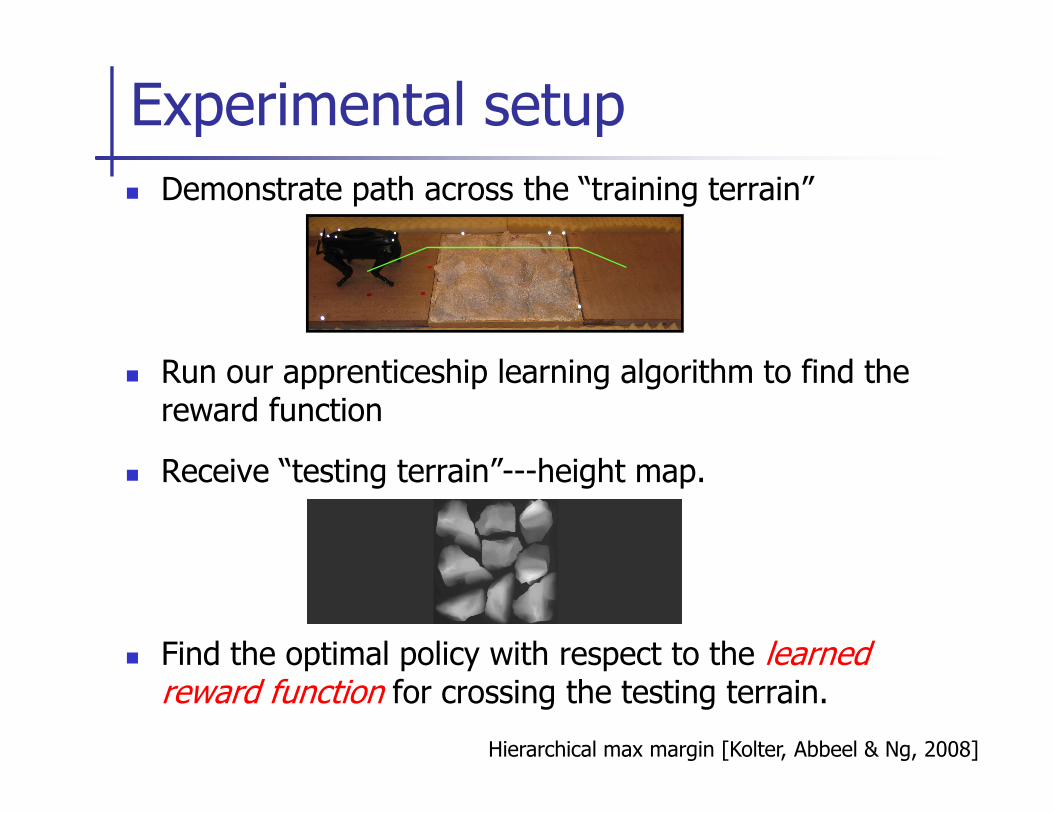
� Demonstrate path across the “training terrain”
� Run our apprenticeship learning algorithm to find the reward function
Experimental setup
reward function
� Receive “testing terrain”---height map.
� Find the optimal policy with respect to the learned reward function for crossing the testing terrain.
Hierarchical max margin [Kolter, Abbeel & Ng, 2008]
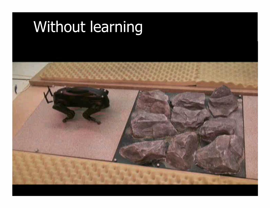
Without learning
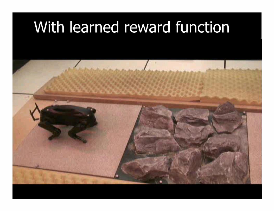
With learned reward function
� Run footstep planner as expert (slow!)
� Run boosted max margin to find a reward function that explains the center of gravity path of the robot (smaller state space)
Quadruped: Ratliff + al, 2007
� At control time: use the learned reward function as a heuristic for A* search when performing footstep-level planning
� Example applications
� Inverse RL vs. behavioral cloning
� Sketch of history of inverse RL
� Mathematical formulations for inverse RL
Summary
� Case studies
� Open directions: Active inverse RL, Inverse RL w.r.t. minmax control, partial observability, learning stage (rather than observing optimal policy), … ?


![FurtherStudiesonAntioxidantPotentialandProtectionof ...downloads.hindawi.com/journals/jdr/2007/015803.pdf · formulations [13, 14]. Ayurveda also describes vidanga as pungent and](https://static.fdocument.org/doc/165x107/5e983cb5ea21fc1c66732cb3/furtherstudiesonantioxidantpotentialandprotectionof-formulations-13-14-ayurveda.jpg)