Inverse Gaussian Distribution Alessia Dorigoni

The main properties The standard form of the Inverse Gaussian distribution is given by the probability density function (PDF):

! ! =λ

2!!!  !"#−! ! − µμ !

2!!!

for x > 0, λ > 0 and µ > 0. But we have different variations of it. In Deniz, Sarabia and Calderin-Ojeda (2005), for example, they mixed the p negative binomial parameter with an inverse Gaussian distribution considering the reparameterization p = exp(−λ) proponing a binomial-inverse Gaussian distribution interesting to study insurance-premiums calculation and their robustness. Alanko and Duffy (1996) developed a compound binomial distribution mixing the binomial parameter using the gamma and inverse Gaussian distributions. Usually, in finance, the binomial options pricing model (BOPM) provides a generalizable numerical method for the valuation of options. There have been several generalizations of Inverse Gaussian proposed in the literature. In the Chou and Huang’s generalization (2004) the pdf is given by ! ! = !!!!! !"# −!" −

!!

for x > 0, α > 0, p > 0 and q > 0 An alternative Inverse Gaussian distribution was proposed by Nadarajah (2009) and the pdf given by

! ! = !!!!!!! !" +!!

for x > 0, α > 0, c > 0 and ν > 0, “where C denotes the normalizing constant and

!! ! =!!!

2!г(! + 12)!! − 1 !!!!

!

!exp −!" !"

is the modified Bessel function of the third kind”. Considering the canonical pdf we have a continuous probability distributions with two parameters: µ is the mean and λ is the shape parameter. The function has support on (0,∞) for X ∼ IG (µ, λ). The effect of the parameters is evident: increasing µ has the effect of changing the mean of the distribution while increasing λ has the effect of changing the shape of the function (see Figure 1 from Giner and Smyth, 2014).

Mean ! ! = !

!1! =

1! +

1!

Mode ! 1+

9!!

4!!

!!−3!2!

Variance !"# ! =!!!

!"#1! =

1!" +

2!!

Skewness

3!!

!!

Ex Kurtosis 15!!

MGF !

!! 1− 1−

2!!!!

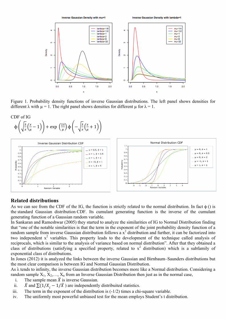
Figure 1. Probability density functions of inverse Gaussian distributions. The left panel shows densities for different λ with µ = 1. The right panel shows densities for different µ for λ = 1. CDF of IG

ɸ !!

!!− 1 + exp   !!

!ɸ − !

!!!+ 1

Related distributions As we can see from the CDF of the IG, the function is strictly related to the normal distribution. In fact φ () is the standard Gaussian distribution CDF. Its cumulant generating function is the inverse of the cumulant generating function of a Gaussian random variable. In Sankaran and Rameshwar (2005) they started to analyze the similarities of IG to Normal Distribution finding that “one of the notable similarities is that the term in the exponent of the joint probability density function of a random sample from inverse Gaussian distribution follows a x2 distribution and further, it can be factorized into two independent x2 variables. This property leads to the development of the technique called analysis of reciprocals, which is similar to the analysis of variance based on normal distribution”. After that they obtained a class of distributions (satisfying a specified property, related to x2 distribution) which is a subfamily of exponential class of distributions. In Jones (2012) it is analyzed the links between the inverse Gaussian and Birnbaum–Saunders distributions but the most clear comparison is between IG and Normal Gaussian Distribution. As λ tends to infinity, the inverse Gaussian distribution becomes more like a Normal distribution. Considering a random sample X1, X2,…, Xn from an Inverse Gaussian Distribution then just as in the normal case,

i. The sample mean ! is inverse Gaussian. ii. ! and (1/!! − 1/! ) are independently distribuited statistics.

iii. The term in the exponent of the distribution is (-1/2) times a chi-square variable. iv. The uniformly most powerful unbiased test for the mean employs Student’s t distribution.

This relation was given in the Theorem 1 in Chhikara and Folks (1989) which establishes a basic relationship between IG and the normal. Genesis and applications especially in economics/management The Inverse Gaussian Distribution was first derived by Schordinger (1915) as the first probability distribution of the first passage time in a linear Brownian motion process with a positive drift. Later, Tweedie (1941) proposed the name Inverse Gaussian because while the Gaussian describes a Brownian Motion's level at a fixed time, the inverse Gaussian describes the distribution of the time a Brownian Motion with positive drift takes to reach a fixed positive level. Tweedie (1957) investigated its basic characteristics, established some distributional properties, and depicted certain analogies between its statistical properties and that of normal distribution. The notion of Brownian motion is applicable in describing the inherent process of many phenomena, particularly in the natural and physical sciences. Because the first passage time of a Brownian motion is distribuited as Inverse Gaussian, it is logical to use it as a lifetime model. The distribution has a wide application area in clinical trials, quality and reliability theory, industrial engineering applications and life tests. The IG distribution is widely used in reliability and survival analysis (Whitmore, 1975; Chhikara and Folks, 1977; Bardsley, 1980; Chhikara, 1989). It is more generally used for modeling non-negative positively skewed data because of its connections to exponential families and generalized linear models. Most of these applications are base on the idea of first passage time for underlying process (cardiology, hydrology, demography, linguistics, employment service, labor disputes and finance). For the cardiology IG is used to describe cycle time distribution for particles in the blood (Wise, 1975) and for the probability distribution for the time that a particle of a substance remains in the blood, the time distribution. It is used as a purchase incidence model, postulating that the interpurchase times follow an IG (Banerjee and Bhattacharyya 1976). Leonenko, Petherick, Sikorskii (2012) used IG for a model for a risky asset, an investment with a return that is not guaranteed, with dependence in a stock price model. Balakrishna and Rahul (2014) proposed IG distribution for modeling conditional durations in finance. Using data from price duration they proved that IG stochastic conditional duration model provides a choice for analyzing transaction durations in financial time series. IG is used for derivative pricing. once the four moments (mean, variance, skewness and kurtosis) are given, you can fill in the blanks with the NIG and obtain the entire distribution. Liu, Li, Hu (2015) used data set about times to breakdown in minutes of an insulating fluid subjected to high voltage stress assuming that the failure time of the insulating fluid for each group as an IG distribuited random variable since the IG distribution is widely applied as a lifetime model in reliability analysis. In survival analysis also frailty is often used to model heterogeneity between individuals or correlation within clusters. Typically frailty is taken to be a continuous random effect, yielding a continuous mixture distribution for survival times and the gamma distribution is the most commonly used frailty distribution. But in Kheiria, Kimberb Meshkanic, an IG distribution has been used for the two components of the correlated frailty variable and a piecewise constant hazard model has been adopted. IG is used for word frequency distribution (Herdan, 1960), length of employee service (Withmore, 1979), net maternity function (Hadwiger, 1940), wind speed and energy evaluation (Bardsley, 1980) in Chhikara and Folks (1989) and as a model for response times in psychology (Schwarz, 2001) How to determine probabilities using a computer The R programming language has software for IG distribution. In Giner and Smyth (2014) they used the monotonic Newton iteration, implemented in the qinvgauss function of the R package statmod to compute quantiles of inverse Gaussian distributions. The following is minimal R code to implement the monotonic Newton iteration (to compute quantiles of the IG distribution). We are interested only in the first part about PDF and CDF. The code assumes that x and q values are positive and the probabilities are strictly between 0 and 1. The first argument is assumed to be a vector, whereas the parameters µ and φ are scalars. dinvgauss <- function(x, mu=1, phi=1) # Probability density function of inverse Gaussian distribution d <- (-log(phi)-log(2*pi)-3*log(x))/2-((x-mu)/mu)^2/(2*phi*x) exp(d) pinvgauss <- function(q, mu=1, phi=1) # Cumulative distribution function of inverse Gaussian distribution

q <- q/mu phi <- phi*mu pq <- sqrt(phi*q) pnorm((q-1)/pq) + exp( 2/phi + pnorm(-(q+1)/pq,log.p=TRUE) )

The sample code in Java for generating random variates from an inverse-Gaussian distribution

References Alanko, T., Duffy, J.C., (1996). Compound binomial distribution for modelling consumption data. The Statistician 45 (3), 269–286. Balakrishna, N., Rahul, T. (2014). Inverse Gaussian Distribution for Modeling Conditional Durations in Finance. Communications in Statistics - Simulation and Computation, 43:3, 476-486. Banerjee and Bhattacharyya (1976). A Purchase Incidence Model With Inverse Gaussian Interpurchase Times. Journal of the American Statistical Association, 71, 823–829 Chhikara, R.S., Folks, J.L. (1989). The inverse gaussian distribution. Statistics: textbook and monographs. Chou, C.-W., Huang, W.-J. (2004). On characterizations of the gamma and generalized inverse Gaussian distributions, Statistics and Probability Letters 69 381–388. Deniza, E. G., Sarabiab, J.M., Ojedaa, E. C. (2008). Univariate and multivariate versions of the negative binomial-inverse Gaussian distributions with applications. Insurance: Mathematics and Economics 42 39–49. Giner, G., Smyth, G. K. (2014). A Monotonically Convergent Newton Iteration for the Quantiles of any Unimodal Distribution, with Application to the Inverse Gaussian Distribution Gupta, R.C., Kundu, D. (2011). Weighted inverse Gaussian – a versatile lifetime model. Journal of Applied Statistics, 38:12, 2695-2708. Jones, M.C. (2012). Relationships between distributions with certain symmetries. Statistics and Probability Letters 82 1737–1744. Kheiria, S., Kimberb, A., Meshkanic, M. R. (2007). Computational Statistics & Data Analysis 51 5317 – 5326. Lemontea, A.J., Cordeiro, G.M. (2011). The exponentiated generalized inverse Gaussian distribution. Statistics and Probability Letters 81 506–517 Leonenkoa, N.N., Petherick, S., Sikorskii, A. (2012). A normal inverse Gaussian model for a risky asset with dependence. Statistics and Probability Letters 82 109-115. Leydold, J., Hörmann, W. (2011). Generating generalized inverse Gaussian random variates by fast inversion. Computational Statistics and Data Analysis 55 213_217. Liu, X., Li, N., Hu, Y. (2015). Combining inferences on the common mean of several inverse Gaussian distributions based on confidence distribution. Statistics and Probability Letters 105 136–142. Nadarajah, S. (2009). An alternative inverse Gaussian distribution. Mathematics and Computers in Simulation 79 1721–1729. Sankaran, P.G., Rameshwar, D. G. (2005). A General Class of Distributions: Properties and Applications, Communications in Statistics - Theory and Methods, 34:11, 2089-209. Schrodinger E., (1915). Zur Theorie der Fall-und Steigversuche an Teilchen mit Brownscher Bewegung, Physikalische Zeitschrift 16, 289-295. Tweedie M.C.K., (1957). Statistical properties of inverse Gaussian distributions I, II, Annals of Mathematical Statistics 28, 362{377. Vladimirescu, I., Tunaru, R. (2003). Estimation functions and uniformly most powerful tests for inverse Gaussian distribution. Comment.Math.Univ.Carolinae 44,1 153-164. Wise, M. E. (1975). Skew Distributions in Biomedicine Including some with Negative Powers of Time. Volume 17 of the series NATO Advanced Study Institutes Series pp 241-262.