Introduction - TWMS) J

TWMS J. Pure Appl. Math. V.9, N.2, 2018, pp.123-134

SKEW GENERALIZED QUASI-CYCLIC CODES

TAHER ABUALRUB1, MARTIANUS FREDERIC EZERMAN2

PADMAPANI SENEVIRATNE3, PATRICK SOLE4

Abstract. This article discusses skew generalized quasi-cyclic codes over any finite field F with

Galois automorphism θ. This is a generalization of both quasi-cyclic codes and skew polynomial

codes. These codes have an added advantage over quasi-cyclic codes since their lengths do not

have to be multiples of the index.

After a brief description of the skew polynomial ring F[x; θ], we show that a skew generalized

quasi-cyclic code C is a left submodule of R1×R2× . . .×Rℓ, where Ri , F[x; θ]/(xmi −1), with

|⟨θ⟩| = m and m divides mi for all i ∈ {1, . . . , ℓ}. This description provides a direct construction

of many codes with best-known parameters over GF (4). As a byproduct, some good asymmetric

quantum codes detecting single bit-flip error can be derived from the constructed codes.

Keywords: generalized skew quasi-cyclic codes, skew polynomial codes, quasi-cyclic codes, quan-

tum CSS codes.

AMS Subject Classification: 94B05, 81P70, 16S36.

1. Introduction

One of the most important problems in error-correcting codes is to construct codes with good

parameters, such as having a large minimum Hamming distance for a given dimension. Such a

code is capable of detecting and correcting a good number of errors. One class of codes that has

been studied in the literature is quasi-cyclic (QC) codes. QC codes of index ℓ over a finite field

F are linear codes where the cyclic shift of any codeword by ℓ positions is another codeword. QC

codes of index ℓ = 1 are the well-known cyclic codes. The importance of the family of QC codes

has been shown in, e.g., [6], [18], [19], [20], [24], and [28]. Many of the optimal and currently

best-known linear codes are QC codes as established in, e.g., [6], [12], [13], [14], and [26].

Some recent works in the literature, such as [1], [3], [4], [10], and [25], focussed on the construc-

tion of error-correcting codes using non-commutative rings. D. Boucher et al. in [3] and in [4],

generalized the notion of cyclic codes by using generator polynomials in a non-commutative

polynomial ring called skew polynomial ring. They gave some examples of skew cyclic codes

with minimum distances as good as the best-known comparable linear codes of the same lengths

and dimensions. Extending the non-commutative framework to quasi-cyclic codes, Abualrub et

al. derived many new optimal linear codes from skew QC codes in [1].

Siap and Kulhan [27] introduced the concept of generalized quasi-cyclic (GQC) codes over

finite fields. These codes are generalization of QC codes. Esmaili and Yari [7] gave examples of

1Department of Mathematics and Statistics, American University of Sharjah, Sharjah, UAE2School of Physical and Mathematical Sciences, Nanyang Technological University, Singapore3Department of Mathematics, Texas A&M University-Commerce, TX, USA4 CNRS/LAGA, University of Paris 8, 93 526 Saint-Denis, France

e-mail: [email protected], [email protected], [email protected],

[email protected]

Manuscript received March 2016.

123

124 TWMS J. PURE APPL. MATH., V.9, N.2, 2018

GQC codes with parameters equalling those of the then best-known linear codes. J. Gao et al.

in [10] studied skew GQC codes using the Chinese Remainder Theorem.

In this work we study skew GQC codes and give a direct approach to the construction of

these codes. We will show that both classical and quantum codes with good parameters can

be derived from them. The paper is organized as follows. After this introduction, we give a

preliminary introduction on the skew polynomial ring F[x; θ] in Section 2. Properties of skew

GQC codes and their duals over finite fields are discussed in Section 2. Section 3 provides our

search results for good classical and quantum codes that can be derived from skew GQC codes.

Section 4 wraps the paper up with conclusions and open problems. A last section is dedicated

to Acknowledgements.

2. The skew polynomial ring F [x, θ]

To make this work self-contained, we begin with a brief introduction on skew polynomial rings

over finite fields and their properties.

Let F be any finite field of characteristic p. Let θ be an automorphism of F with |⟨θ⟩| = m.

Let K be the subfield of F fixed by θ. Then, [F : K] = m, K = GF (pt), and F = GF (q = ptm).

Since θ fixes K, θ(a) = aptfor all a ∈ F.

Definition 2.1. Keeping the above notations, a skew polynomial set F[x; θ] is given by

F[x; θ] = {f(x) = a0 + a1x+ . . .+ anxn with ai ∈ F for all i ∈ {0, 1, . . . , n}} .

Addition is defined in the usual manner, while multiplication is associative, distributive on the

addition, and follows the rule

(axi) (bxj) = a θi(b) xi+j.

Theorem 2.1. [21] The set F[x; θ] with respect to addition and multiplication in Definition 2.1.

forms a non-commutative ring called a skew polynomial ring.

Some facts are straightforward. The ring F[x; θ] has no nonzero zero-divisors. Its units are the

units of F. Due to how the operations are defined, deg(f(x)+g(x)) ≤ max{deg(f(x)), deg(g(x))}and deg(f(x)g(x)) = deg(f(x))+deg(g(x)). The ring F[x; θ] was introduced by Ore [22] in 1933,

and a complete treatment of this ring can be found in [17] and in [21].

Theorem 2.2. [21, The Right Division Algoritheorem]. For f(x) = 0 and g(x) in F[x; θ] thereexist unique polynomials q(x) and r(x) in F[x; θ] such that

g(x) = q(x)f(x) + r(x) with deg(r(x)) < deg(f(x)).

The above result is called division on the right by f(x). A similar result holds regarding

division on the left by f(x). Applying the division algoritheorem one can prove the following

result.

Theorem 2.3. [17] The ring F[x; θ] is a noncommutative principal left and right ideal ring.

Any two-sided ideal must be generated by

f(x) = (a0 + a1xm + a2x

2m + . . .+ arxrm) xe, where |⟨θ⟩| = m.

In particular, the ideal generated by (xs − 1) with m | s is a two-sided ideal.

T. ABUALRUB et al: SKEW GENERALIZED QUASI-CYCLIC CODES 125

The next two results state some properties of the center Z(F[x; θ]) of F[x; θ].Lemma 2.1. [1, Lemma 1] If m | s, then Z(F[x; θ]) contains (xs − 1).

Lemma 2.2. [5, Lemma 7] If g(x) h(x) ∈ Z(F[x; θ]), then g(x)h(x) = h(x)g(x).

From Lemmas 2 and 2, we may conclude that the factors of xs − 1 commute. Thus, if f(x) is

a left divisor of xs − 1, then it is also a right divisor. This fact helps in reducing the complexity

of factoring xs − 1 in F[x; θ]. Henceforth, we say divisors or factors of xs − 1 without specifying

left or right.

Definition 2.2. We say that f(x) is a right multiple of h(x) if there exists g(x) such that

f(x) = h(x) g(x). When this is the case, h(x) is called a left divisor of f(x).

Definition 2.3. A monic polynomial h(x) is the greatest common left divisor of a(x) and

b(x), denoted by gcld(a(x), b(x)), if h(x) is a left divisor of both a(x) and b(x) and if, for any

other left divisor e(x) of a(x) and b(x), there exists k(x) satisfying h(x) = e(x) k(x).

Since θ is an automorphism of F, then the greatest common right divisor gcrd of a(x) and b(x)

is a monic polynomial defined analogously. The least common left multiple, denoted by lclm,

and least common right multiple, denoted by lcrm, are well-defined in F[x; θ].

3. Skew generalized quasi cyclic codes

In this section we define skew generalized quasi-cyclic (GQC) codes and establish their most

important properties.

Definition 3.1. Let F be a finite field of characteristic p with q = pmt elements, and let θ be

an automorphism of F with |⟨θ⟩| = m. Let (a1, a2, . . . , an) ∈ Fn. Define the function

T : Fn → Fn by (a1, a2, . . . , an) 7→ (θ(an), θ(a1), . . . , θ(an−1)). (1)

Let m1,m2, . . . ,mℓ be positive integers with m | mi for all i ∈ {1, 2, . . . , ℓ} and n :=∑ℓ

i=1mi.

A subset C of Fm1 × Fm2 × . . .× Fmℓ is called a skew generalized quasi-cyclic code of length n

and index ℓ (or a skew ℓ-GQC code) if both of the following conditions hold.

(1) The code C is a subspace of Fm1 × Fm2 × . . .× Fmℓ.

(2) Let vj , (vj,1, vj,2, . . . , vj,mj ) ∈ Fmj for all j ∈ {1, . . . , ℓ}. If v = (v1,v2, . . . ,vℓ) ∈ C,

then T(v) = (T(v1),T(v2), . . . ,T(vℓ)) ∈ C.

Thus, skew ℓ-GQC codes are linear codes that are closed under skew quasi-cyclic shift. If θ is

the identity map, then skew ℓ-GQC codes are just the standard GQC codes over F. For brevity,henceforth we assume that n :=

∑ℓi=1mi, and m | mi for all i ∈ {1, 2, . . . , ℓ}.

With each vj = (vj,1, vj,2, . . . , vj,mj ) ∈ Fmj we associate the polynomial vj(x) =∑mj

i=1 vj,ixi−1

for all j ∈ {1, . . . , ℓ}. This gives a one to one correspondence between Fm1 × Fm2 × . . . × Fmℓ

and the ring R = R1 ×R2 × . . .×Rℓ where Rj , F[x; θ]/(xmj − 1) for all j ∈ {1, . . . , ℓ}. In fact,

the following result is straightforward from the definition

Theorem 3.1. Let Rj , F[x; θ]/(xmj − 1) and g(x) ∈ F[x; θ]. Then the ring

R , R1 ×R2 × . . .×Rℓ

is a left F[x; θ]-module with multiplication defined by

g(x)(f1(x) + (xm1 − 1), . . . , fℓ(x) + (xmℓ − 1))

= (g(x)f1(x) + (xm1 − 1), . . . , g(x)fℓ(x) + (xmℓ − 1)). (2)


At this point it is easy to see that Definition 3 is equivalent to the following definition.

Definition 3.2. ([10, Definition 3.1].) A subset C is called a skew ℓ-GQC code of length n if

C is a left F[x; θ]-submodule of R.

We say that C is a 1-generator skew ℓ-GQC code if it has the form

C = {f(x)(s1(x), s2(x), . . . , sℓ(x)) : f(x) ∈ F[x; θ] and sj(x) ∈ Rj} . (3)

We often denote such a code by C = ⟨S(x)⟩ where S(x) := (s1(x), . . . , sℓ(x)). The following

lemma was established in [10, Section 4].

Lemma 3.1. Let C be a 1-generator skew ℓ-GQC code of length n. Then there exist polyno-

mials gi(x) and pi(x) ∈ Ri such that gi(x) divides xmi − 1 and

C = ⟨(p1(x)g1(x), p2(x)g2(x), . . . , pℓ(x)gℓ(x))⟩.

The next result is similar to [10, Theorem 4.2]. Here we give a direct proof of the theorem

instead of via the parity-check polynomial as was done in the said reference.

Theorem 3.2. Let C be a skew ℓ-GQC code C of length n given by

C = ⟨(p1(x)g1(x), p2(x)g2(x), . . . , pℓ(x)gℓ(x))⟩

and let µi(x) := gcld (pi(x)gi(x), xmi − 1). Write xmi − 1 = βi(x) µi(x) = µi(x) βi(x), and

define u(x) := lclm (β1(x), β2(x), . . . , βℓ(x)). Then dim(C) = deg(u(x)).

Proof. Since µi(x) = gcld (pi(x)gi(x), xmi − 1), there exist αi(x) and βi(x) such that

pi(x) gi(x) = µi(x) αi(x) and xmi − 1 = βi(x) µi(x) = µi(x) βi(x). (4)

Hence, we can write

βi(x) =xmi − 1

µi(x). (5)

By definition, for each i there exists γi(x) for which u(x) = γi(x) βi(x). By Eq. (5),

u(x) = γi(x)xmi − 1

µi(x).

Suppose c(x) = f(x) (p1(x) g1(x), . . . , pℓ(x) gℓ(x)) ∈ C. Applying the right division algo-

ritheorem, there exist q(x) and ri(x), for each i, such that

f(x) = q(x) u(x) + ri(x) with 0 = ri(x) or deg(ri(x)) < deg(u(x)).

This implies that

f(x) pi(x) gi(x) = (q(x) u(x) + ri(x)) pi(x) gi(x) = q(x) u(x) pi(x) gi(x) + ri(x) pi(x) gi(x)

= q(x) γi(x)xmi − 1

µi(x)µi(x) αi(x) + ri(x) pi(x) gi(x)

≡ ri(x) pi(x) gi(x) modulo (xmi − 1).

Using the notations p(x) := (p1(x), . . . , pℓ(x)), g(x) := (g1(x), . . . , gℓ(x)), and

p(x) g(x) , (p1(x) g1(x), p2(x) g2(x), . . . , pℓ(x) gℓ(x)),

we obtain C = ⟨S⟩ with S ={xj p(x) g(x)

}deg(u(x))−1

j=0. Next, we show that S is linearly inde-

pendent.

Suppose, for a contradiction, that there exists f(x) ∈ F[x; θ] with deg f (x) < deg u (x) satis-

fying

f(x) (p1(x) g1(x), p2(x) g2(x), . . . , pℓ(x) gℓ(x)) = (0, 0, . . . , 0).


Hence,

f(x) pi(x) gi(x) = yi(x) (xmi − 1) for some yi(x). (6)

Since µi(x) = gcld (pi(x)gi(x), xmi − 1), there exist polynomials w1(x) and w2(x) satisfying

f(x) pi(x) gi(x) w1(x) + f(x) (xmi − 1) w2(x) = f(x) µi(x).

By Eq. (6) and since (xmi − 1) ∈ Z(F[x; θ]), we can write

(yi(x) w1(x) + f(x) w2(x)) (xmi − 1) = f(x) µi(x).

Now, Eq. (4) allows us to infer that (yi(x) w1(x)+f(x) w2(x)) βi(x) µi(x) = f(x) µi(x), implying

that (yi(x) w1(x)+ f(x) w2(x)) βi(x) = f(x). Thus, f(x) is a common left multiple of βi(x) for

all i. Hence, there exists d(x) such that f(x) = d(x) u(x) since u(x) = lclm (β1(x), . . . , βℓ(x)).

This is a contradiction since deg(f(x)) < deg(u(x)). �

Definition 3.3. Let C be a skew ℓ-GQC code C of length n. Let vi = (vi,1, . . . , vi,mi) ∈ Fmi.

The dual code C⊥ of C is given by

C⊥ =

{v = (v1, . . . ,vℓ) ∈ Fm1 × Fm2 × . . .× Fmℓ : ⟨v, c⟩ :=

ℓ∑i=1

mi∑j=1

vi,jci,j = 0

}.

The next results establishes that if C is a skew ℓ-GQC code then C⊥ is also a skew ℓ-GQC

code.

Theorem 3.3. Let C be a skew GQC code of length n = m1 +m2 + . . .mℓ and index ℓ. Then

C⊥ is also a skew GQC code of length n and index ℓ.

Proof. Let

a = (a1, . . . ,aℓ) = (a1,0, a1,1, . . . , a1,m1−1, a2,0, a2,1, . . . , a2,m2−1, . . . , aℓ,0, aℓ,1, . . . , aℓ,mℓ−1) ∈ C⊥.

To show that C⊥ is a skew GQC code of length n = m1 +m2 + . . .+mℓ and index ℓ, it suffices

to show that

T(a) = (θ(a1,m1−1), θ(a1,0), . . . , θ(a1,m1−2), θ(a2,m2−1), θ(a2,0), . . . , θ(a2,m2−2), . . . ,

θ(aℓ,mℓ−1), θ(aℓ,0), . . . , θ(aℓ,mℓ−2)) ∈ C⊥,

i.e., for any

c = (c1, . . . , cℓ) = (c1,0, c1,1, . . . , c1,m1−1, c2,0, c2,1, . . . , c2,m2−1, . . . , cℓ,0, cℓ,1, . . . , cℓ,mℓ−1) ∈ C

we must show that ⟨T(a), c⟩ = 0. Writing explicitly,

⟨T(a), c⟩ =c1,0θ(a1,m1−1) + c1,1θ(a1,0) + . . .+ c1,m1−1θ(a1,m1−2) + . . .+

cℓ,0θ(aℓ,mℓ−1) + cℓ,1θ(aℓ,0) + . . .+ cℓ,mℓ−1θ(aℓ,mℓ−2). (7)

Since C is skew GQC code, Tk(c) ∈ C. Let M := lcm(m1,m2, . . . ,mℓ). Since |⟨θ⟩| = m and m |mi for all i ∈ {1, . . . , ℓ}, we know that m | M . Hence, θM (x) = x for any x, θM−1(x) = θ−1(x),

and TM (c) = c. Thus,

TM−1(c) = (θ−1(c1,1), θ−1(c1,2), . . . , θ

−1(c1,m1−1), θ−1(c1,0), . . . ,

θ−1(cℓ,1), θ−1(cℓ,2), . . . , θ

−1(cℓ,mℓ−1), θ−1(cℓ,0)).

Since C is a skew GQC code, we have⟨a,TM−1(c)

⟩= 0. Hence,

a1,0θ−1(c1,1) + a1,1θ

−1(c1,2) + . . .+ a1,m1−1θ−1(c1,0) + . . .+

aℓ,0θ−1(cℓ,1) + aℓ,1θ

−1(cℓ,2) + . . .+ aℓ,mℓ−1θ−1(cℓ,0) = 0. (8)


Apply θ to both sides of Eq. (8) to get

c1,1θ(a1,0) + c1,2θ(a1,1) + . . .+ c1,0θ(a1,m1−1) + . . .+

cℓ,1θ(aℓ,0) + cℓ,2θ(aℓ,1) + . . .+ cℓ,0θ(aℓ,mℓ−1) = 0. (9)

Notice that the left hand side of Eq. (9) is the right hand side of Eq. (7) after some rearrangement.

Therefore, C⊥ is indeed a skew GQC code of length n = m1 +m2 + . . .+mℓ and index ℓ. �

Remark 3.1. Theorem 3.3 states that if C is a skew ℓ-GQC code, then C⊥ is also a skew

ℓ-GQC code. Note, however, that if C is a 1-generator skew ℓ-GQC code, then C⊥ is not

necessarily 1-generator as well.

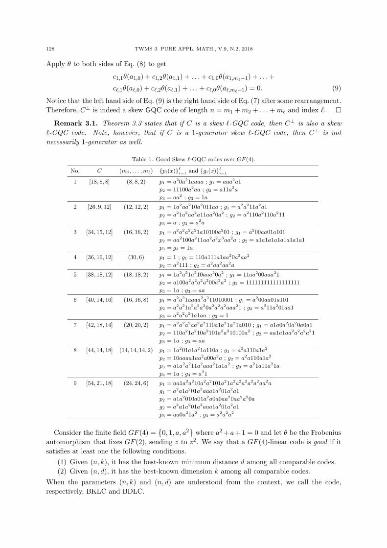
Table 1. Good Skew ℓ-GQC codes over GF (4).

No. C (m1, . . . ,mℓ) {pi(x)}ℓi=1 and {gi(x)}ℓi=1

1 [18, 8, 8] (8, 8, 2) p1 = a20a21aaaa ; g1 = aaa2a1

p2 = 11100a2aa ; g2 = a11a2a

p3 = aa2 ; g3 = 1a

2 [26, 9, 12] (12, 12, 2) p1 = 1a2aa210a2011aa ; g1 = a2a211a2a1

p2 = a21a2aa2a11aa20a2 ; g2 = a2110a2110a211

p3 = a ; g3 = a2a

3 [34, 15, 12] (16, 16, 2) p1 = a2a2a2a21a10100a201 ; g1 = a200aa01a101

p2 = aa2100a211aa2a2x3aa2a ; g2 = a1a1a1a1a1a1a1a1

p3 = g3 = 1a

4 [36, 16, 12] (30, 6) p1 = 1 ; g1 = 110a111a1aa20a2aa2

p2 = a2111 ; g2 = a2aa2aa2a

5 [38, 18, 12] (18, 18, 2) p1 = 1a2a21a210aaa20a2 ; g1 = 11aa200aaa21

p2 = a100a2a2a2a200a2a2 ; g2 = 111111111111111111

p3 = 1a ; g3 = aa

6 [40, 14, 16] (16, 16, 8) p1 = a2a21aaaa2a211010001 ; g1 = a200aa01a101

p2 = a2a21a2a2a20a2a2a2aaa21 ; g2 = a211a201aa1

p3 = a2a2a21a1aa ; g3 = 1

7 [42, 18, 14] (20, 20, 2) p1 = a2a2a2aa2a2110a1a21a21a010 ; g1 = a1a0a20a20a0a1

p2 = 110a21a210a2101a2a210100a2 ; g2 = aa1a1aa2a2a2a21

p3 = 1a ; g3 = aa

8 [44, 14, 18] (14, 14, 14, 2) p1 = 1a201a1a21a110a ; g1 = a2a110a1a2

p2 = 10aaaa1aa2a00a2a ; g2 = a2a110a1a2

p3 = a1a2a211a2aaa21a1a2 ; g3 = a21a11a21a

p4 = 1a ; g4 = a21

9 [54, 21, 18] (24, 24, 6) p1 = aa1a2a210a2a2101a21a2a2a2a2a2aa2a

g1 = a2a1a201a2aaa1a201a2a1

p2 = a1a2010a01a2a0a0aa20aa2a20a

g2 = a2a1a201a2aaa1a201a2a1

p3 = aa0a21a2 ; g3 = a2a2a2

Consider the finite field GF (4) ={0, 1, a, a2

}where a2+a+1 = 0 and let θ be the Frobenius

automorphism that fixes GF (2), sending z to z2. We say that a GF (4)-linear code is good if it

satisfies at least one the following conditions.

(1) Given (n, k), it has the best-known minimum distance d among all comparable codes.

(2) Given (n, d), it has the best-known dimension k among all comparable codes.

When the parameters (n, k) and (n, d) are understood from the context, we call the code,

respectively, BKLC and BDLC.


This section contains three distinct but related search results. Good skew ℓ-GQC codes found

are discussed in the first subsection. The second one gives the results upon applying shortening

and puncturing methods. To highlight the benefit of constructing skew ℓ-GQC codes we show

how to derive some asymmetric quantum codes detecting single bit-flip error in the third one.

These quantum codes cannot presently be derived from the BKLC and BDLC codes stored in

the MAGMA database or the codes recorded in the Grassl Table [11].

3.1. Good Skew ℓ-GQC codes over GF (4). We wrote a program in MAGMA (Ver. 2.20) [2]

to search for good GF (4)-linear skew ℓ-GQC codes based on the results obtained in previous

sections. The program first generates positive even integers m1, . . . ,mℓ. It then searches for a

divisor gi(x) of xmi − 1 in F[x; θ]. Next, it looks for polynomials pi(x) so that the skew ℓ-GQC

code of the form

C := ⟨p1(x) g1(x), p2(x) g2(x), . . . , pℓ(x) gℓ(x)⟩

has a large minimum distance d. The product pi(x) gi(x) is then computed modulo (xmi − 1).

For ease of verification, when presenting the good codes that the program finds we list down

pi(x) and gi(x). The polynomials are represented by a sequence of coefficients of decreasing

powers. For example, the sequence 1a0a20a represents the polynomial x5+ax4+a2x2+a. Table

1 lists down skew ℓ-GQC codes having the parameters specified by BKLC(GF (4), n, k). They

are, however, not BDLC. The main advantage of these codes over most of the corresponding

codes in the Grassl Table is that they can be directly constructed as opposed to being obtained

through some rather ad hoc steps.

Example 3.1. Consider the skew 3-GQC [18, 8, 8] code C listed as Entry 1 in Table 1. Note

that d(C) = 8, equaling the minimum distance specified by BKLC(GF (4), 18, 8). The best-

known code in the Grassl Table was obtained indirectly in two steps. First, an [18, 9, 8]4-code is

constructed from a stored generator matrix. Taking a subcode of the resulting code then yields

an [18, 8, 8]4-code.

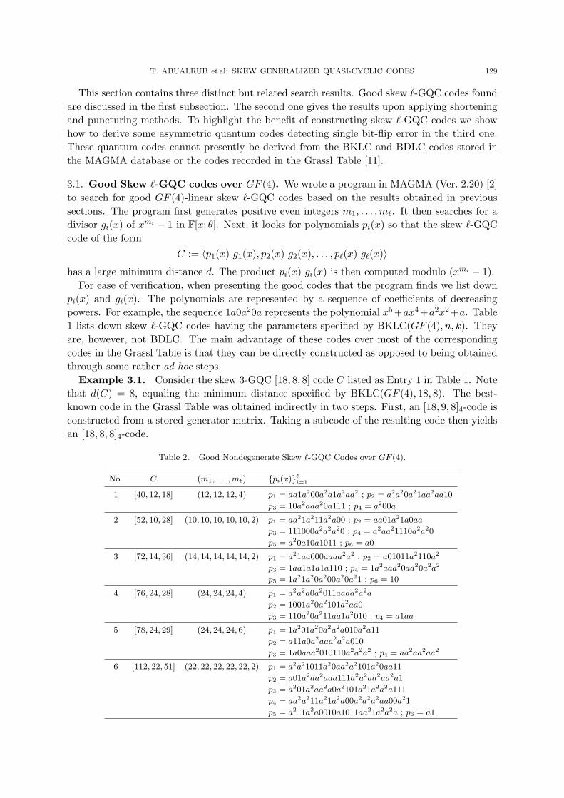
Table 2. Good Nondegenerate Skew ℓ-GQC Codes over GF (4).

No. C (m1, . . . ,mℓ) {pi(x)}ℓi=1

1 [40, 12, 18] (12, 12, 12, 4) p1 = aa1a200a2a1a2aa2 ; p2 = a2a20a21aa2aa10

p3 = 10a2aaa20a111 ; p4 = a200a

2 [52, 10, 28] (10, 10, 10, 10, 10, 2) p1 = aa21a211a2a00 ; p2 = aa01a21a0aa

p3 = 111000a2a2a20 ; p4 = a2aa21110a2a20

p5 = a20a10a1011 ; p6 = a0

3 [72, 14, 36] (14, 14, 14, 14, 14, 2) p1 = a21aa000aaaa2a2 ; p2 = a01011a2110a2

p3 = 1aa1a1a1a110 ; p4 = 1a2aaa20aa20a2a2

p5 = 1a21a20a200a20a21 ; p6 = 10

4 [76, 24, 28] (24, 24, 24, 4) p1 = a2a2a0a2011aaaa2a2a

p2 = 1001a20a2101a2aa0

p3 = 110a20a211aa1a2010 ; p4 = a1aa

5 [78, 24, 29] (24, 24, 24, 6) p1 = 1a201a20a2a2a010a2a11

p2 = a11a0a2aaa2a2a010

p3 = 1a0aaa2010110a2a2a2 ; p4 = aa2aa2aa2

6 [112, 22, 51] (22, 22, 22, 22, 22, 2) p1 = a2a21011a20aa2a2101a20aa11

p2 = a01a2aa2aaa111a2a2aa2aa2a1

p3 = a201a2aa2a0a2101a21a2a2a111

p4 = aa2a211a21a2a00a2a2a2aa00a21

p5 = a211a2a0010a1011aa21a2a2a ; p6 = a1


It is also possible to construct good skew ℓ-GQC codes having the trivial factor g(x) = 1.

They are of the form

C := ⟨p1(x), p2(x), . . . , pℓ(x)⟩ .Following [1], these codes are called non-degenerate skew ℓ-GQC codes. Table 2 presents such

codes found in our search. They all satisfy both the BKLC and the BDLC conditions, except for

Entry 4, which is only BKLC, since the largest known dimension for (n = 76, d = 28) is k = 26.

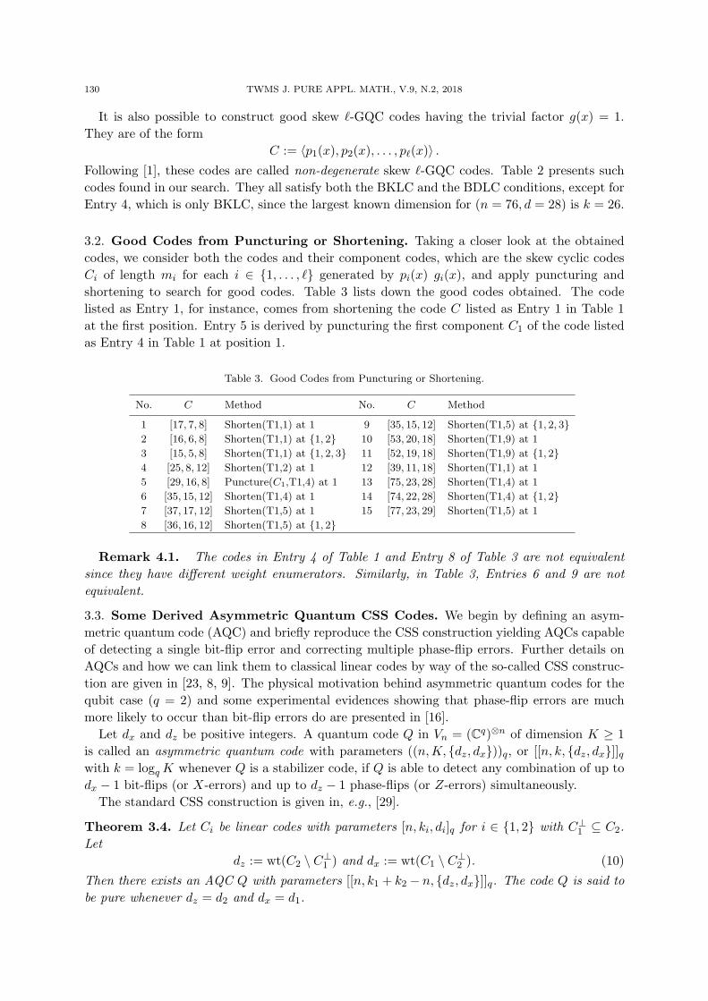
3.2. Good Codes from Puncturing or Shortening. Taking a closer look at the obtained

codes, we consider both the codes and their component codes, which are the skew cyclic codes

Ci of length mi for each i ∈ {1, . . . , ℓ} generated by pi(x) gi(x), and apply puncturing and

shortening to search for good codes. Table 3 lists down the good codes obtained. The code

listed as Entry 1, for instance, comes from shortening the code C listed as Entry 1 in Table 1

at the first position. Entry 5 is derived by puncturing the first component C1 of the code listed

as Entry 4 in Table 1 at position 1.

Table 3. Good Codes from Puncturing or Shortening.

No. C Method No. C Method

1 [17, 7, 8] Shorten(T1,1) at 1 9 [35, 15, 12] Shorten(T1,5) at {1, 2, 3}2 [16, 6, 8] Shorten(T1,1) at {1, 2} 10 [53, 20, 18] Shorten(T1,9) at 1

3 [15, 5, 8] Shorten(T1,1) at {1, 2, 3} 11 [52, 19, 18] Shorten(T1,9) at {1, 2}4 [25, 8, 12] Shorten(T1,2) at 1 12 [39, 11, 18] Shorten(T1,1) at 1

5 [29, 16, 8] Puncture(C1,T1,4) at 1 13 [75, 23, 28] Shorten(T1,4) at 1

6 [35, 15, 12] Shorten(T1,4) at 1 14 [74, 22, 28] Shorten(T1,4) at {1, 2}7 [37, 17, 12] Shorten(T1,5) at 1 15 [77, 23, 29] Shorten(T1,5) at 1

8 [36, 16, 12] Shorten(T1,5) at {1, 2}

Remark 4.1. The codes in Entry 4 of Table 1 and Entry 8 of Table 3 are not equivalent

since they have different weight enumerators. Similarly, in Table 3, Entries 6 and 9 are not

equivalent.

3.3. Some Derived Asymmetric Quantum CSS Codes. We begin by defining an asym-

metric quantum code (AQC) and briefly reproduce the CSS construction yielding AQCs capable

of detecting a single bit-flip error and correcting multiple phase-flip errors. Further details on

AQCs and how we can link them to classical linear codes by way of the so-called CSS construc-

tion are given in [23, 8, 9]. The physical motivation behind asymmetric quantum codes for the

qubit case (q = 2) and some experimental evidences showing that phase-flip errors are much

more likely to occur than bit-flip errors do are presented in [16].

Let dx and dz be positive integers. A quantum code Q in Vn = (Cq)⊗n of dimension K ≥ 1

is called an asymmetric quantum code with parameters ((n,K, {dz, dx}))q, or [[n, k, {dz, dx}]]qwith k = logq K whenever Q is a stabilizer code, if Q is able to detect any combination of up to

dx − 1 bit-flips (or X-errors) and up to dz − 1 phase-flips (or Z-errors) simultaneously.

The standard CSS construction is given in, e.g., [29].

Theorem 3.4. Let Ci be linear codes with parameters [n, ki, di]q for i ∈ {1, 2} with C⊥1 ⊆ C2.

Let

dz := wt(C2 \ C⊥1 ) and dx := wt(C1 \ C⊥

2 ). (10)

Then there exists an AQC Q with parameters [[n, k1 + k2 − n, {dz, dx}]]q. The code Q is said to

be pure whenever dz = d2 and dx = d1.


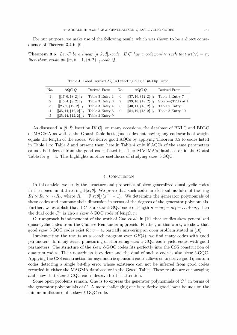
For our purpose, we make use of the following result, which was shown to be a direct conse-

quence of Theorem 3.4 in [9].

Theorem 3.5. Let C be a linear [n, k, d]q-code. If C has a codeword v such that wt(v) = n,

then there exists an [[n, k − 1, {d, 2}]]q-code Q.

Table 4. Good Derived AQCs Detecting Single Bit-Flip Error.

No. AQC Q Derived From No. AQC Q Derived From

1 [[17, 6, {8, 2}]]4 Table 3 Entry 1 6 [[37, 16, {12, 2}]]4 Table 3 Entry 7

2 [[15, 4, {8, 2}]]4 Table 3 Entry 3 7 [[39, 10, {18, 2}]]4 Shorten(T2,1) at 1



5 [[35, 14, {12, 2}]]4 Table 3 Entry 9

As discussed in [9, Subsection IV.C], on many occasions, the database of BKLC and BDLC

of MAGMA as well as the Grassl Table host good codes not having any codewords of weight

equals the length of the codes. We derive good AQCs by applying Theorem 3.5 to codes listed

in Table 1 to Table 3 and present them here in Table 4 only if AQCs of the same parameters

cannot be inferred from the good codes listed in either MAGMA’s database or in the Grassl

Table for q = 4. This highlights another usefulness of studying skew ℓ-GQC.

4. Conclusion

In this article, we study the structure and properties of skew generalized quasi-cyclic codes

in the noncommutative ring F[x; θ]. We prove that such codes are left submodules of the ring

R1 × R2 × · · ·Rℓ, where Ri = F[x; θ]/(xmi − 1). We determine the generator polynomials of

these codes and compute their dimension in terms of the degrees of the generator polynomials.

Further, we establish that if C is a skew ℓ-GQC code of length n = m1 +m2 + . . . +mℓ, then

the dual code C⊥ is also a skew ℓ-GQC code of length n.

Our approach is independent of the work of Gao et al. in [10] that studies skew generalized

quasi-cyclic codes from the Chinese Remainder approach. Further, in this work, we show that

good skew ℓ-GQC codes exist for q = 4, partially answering an open problem stated in [10].

Implementing the results as a search program over GF (4), we find many codes with good

parameters. In many cases, puncturing or shortening skew ℓ-GQC codes yield codes with good

parameters. The structure of the skew ℓ-GQC codes fits perfectly into the CSS construction of

quantum codes. Their nestedness is evident and the dual of such a code is also skew ℓ-GQC.

Applying the CSS construction for asymmetric quantum codes allows us to derive good quantum

codes detecting a single bit-flip error whose existence can not be inferred from good codes

recorded in either the MAGMA database or in the Grassl Table. These results are encouraging

and show that skew ℓ-GQC codes deserve further attention.

Some open problems remain. One is to express the generator polynomials of C⊥ in terms of

the generator polynomials of C. A more challenging one is to derive good lower bounds on the

minimum distance of a skew ℓ-GQC code.


5. Acknowledgment

We thank the anonymous reviewer for the valuable comments that lead us to improve the

paper.

References

[1] Abualrub, T., Ghrayeb, A., Aydin, N., and Siap, I., (2010), On the construction of skew quasi-cyclic codes,

IEEE Trans. Inf. Theory, 56(2), pp.2081-2090.

[2] Bosma, W., Canon, J.J., Playoust, C., (1997), The magma algebra system I: The user language, J. Symbol.

Comput., 24, pp.235-266.

[3] Boucher, D., Geismann, W., Ulmer, F., (2007), Skew-cyclic codes, Appl. Algebra Engrg. Comm. Comput.,

18(4), pp.379-389.

[4] Boucher, D., Sole, P., Ulmer, F., (2008), Skew constacyclic codes over Galois Rings, Adv. Math. Commun.,

2(3), pp.273-292.

[5] Boucher, D., Ulmer, F., (2009), Coding with skew polynomial rings, J. Symbol. Comput., 44, pp.1644-1656.

[6] Chen, Z., (1994), Six new binary quasi-cyclic codes, IEEE Trans. Inf. Theory, 40(5), pp.1666-1667.

[7] Esmaeili, M., Yari, S., (2009), Generalized quasi-cyclic codes: Structural properties and code construction,

Appl. Algebra Engrg. Comm. Comput., 20, pp.159-173.

[8] Ezerman, M.F., Jitman, S., Ling, S., Sole, P., (2011), Additive Asymmetric Quantum Codes, IEEE Trans.

on Information Theory, IT-57, pp.5536-5550.

[9] Ezerman, M.F., Jitman, S., Ling, S., Pasechnik, D.V., (2013), CSS-like constructions of asymmetric quantum

codes, IEEE Trans. Inf. Theory, 59(10), pp.6732-6754.

[10] Gao,J., Shen, L., Fu, F., (2016), A Chinese remainder theorem approach to skew generalized quasi-cyclic

codes over finite fields, Cryptogr. Commun., 8, pp.51-66.

[11] Grassl, M.,(2018), Bounds on the minimum distance of linear codes and quantum codes, Online available at

http://www.codetables.de, accessed on January 2.

[12] Greenough, P.P., Hill, R., (1992), Optimal ternary quasi-cyclic codes, Des. Codes Cryptogr., 2, pp.81-91.

[13] Gulliver, T.A., Bhargava, V.K., (1992), Nine good rate (m − 1)/pm quasi-cyclic codes,”IEEE Trans. Inf.

Theory, 38(4), pp.1366-1369.

[14] Gulliver, T.A., Bhargava, V.K., (1992), Some best rate 1/p and rate (p− 1)/p systematic quasi-cyclic codes

over GF (3) and GF (4), IEEE Trans. Inf. Theory, 38(4), pp.1369-1374.

[15] Hammons A.R., Kumar, P.V., Calderbank, A.R., Sloane, N.J.A., Sole, P., (1994), The Z4-linearity of Ker-

dock, Preparata, Goethals and related codes, IEEE Trans. Inf. Theory, 40, pp.301-319.

[16] Ioffe, L., Mezard, M., (2007), Asymmetric quantum error-correcting codes, Phys. Rev. A, 75(3), pp.32345.

[17] Jacobson, N.,(1943), The Theory of Rings, Amer. Math. Soc. Math., New York.

[18] Kasami, T., (1974), A Gilbert-Varshamov Bound for Quasi-cyclic Codes of Rate 1/2, IEEE Trans. Inf.

Theory, 20, p. 679.

[19] Lally, K., Fitzpatrick, P., (2001), Algebraic structure of quasi-cyclic codes, Discr. Appl. Math., 111, pp.157-

175.

[20] Ling, S., Sole, P., (2001), On the algebraic structure of the quasi-cyclic codes I: Finite fields, IEEE Trans.

Inf. Theory, 47(7), pp.2751-2759.

[21] McDonald, B.R., (1974), Finite Rings with Identity, Marcel Dekker Inc., New York.

[22] Ore, O., (1933), Theory of non-commutative polynomials, Annals of Math., 34, pp.480-508.

[23] Sarvepalli, P.K., Klappenecker, A., Rotteler, M., (2009), Asymmetric quantum codes: Constructions, bounds,

and performance, Proc. Royal Society London A, 465(2105), pp.1645-1672.

[24] Seguin, G.E., Drolet, G., (1990), The theory of 1-generator quasi-cyclic codes, Preprint, Royal Military

College of Canada, Kingston, Ontario.

[25] Siap, I., Abualrub, T., Aydin, N., Seneviratne, P., (2011), Skew cyclic codes of arbitrary lengtht, Int. J. Inf.

Coding Theory, 2(1), pp.10-20.

[26] Siap, I., Aydin, N., Ray-Chaudhuri, D.K., (2000), New ternary quasi-cyclic codes with better minimum

distances, IEEE Trans. Inf. Theory, 46(4), pp.1554-1558.

[27] Siap, I., Kulhan, N., (2005), The structure of generalized quasi cyclic codes, Appl. Math. E-Notes, 5, pp.24-30.

[28] Thomas, K., (1977), Polynomial approach to quasi-cyclic codes, Bul. Cal. Math. Soc., 69, pp.51-59.


[29] Wang, L., Feng, K., Ling, S., Xing, C., (2010), Asymmetric quantum codes: Characterization and construc-

tions, IEEE Trans. Inf. Theory, 56, pp.2938-2945.

Taher Abualrub - is a professor of Mathemat-

ics at the American University of Sharjah. He

received his Master and Ph.D. degrees in Mathe-

matics from the University of Iowa, USA, in Au-

gust 1994 and May 1998, respectively. In 1998 he

joined the American University of Sharjah (AUS)

as an Assistant Professor in the department of

Mathematics and Statistics. Currently, he is a

professor of mathematics at AUS. His research in-

terests include error correcting codes, DNA com-

puting, wavelet theory, and control theory.

Martianus Frederic Ezerman - grew up in

East Java Indonesia. He received the B.A. Phil.

and the B.Sc. Math. degrees in 2005 and the

M.Sc. Math. degree in 2007, all from Ateneo de

Manila University, Philippines, and obtained the

Ph.D. degree in mathematics from Nanyang Tech-

nological University, Singapore in 2011. After re-

search fellowships at Universite Libre de Brux-

elles, Belgium and at the Centre for Quantum

Technologies, National University of Singapore,

he returned in March 2014 to NTU where he is

currently a Senior Research Fellow. His main in-

terests are coding theory, cryptography, and quan-

tum information processing.

Padmapani Seneviratne - received the Ph.D.

degree from Clemson University, South Carolina

in 2007 under the supervision of Dr. Jennifer D.

Key. After graduation, he joined the American

University of Sharjah, UAE, as an Assistant Pro-

fessor and was promoted to Associate Professor

in 2014. He is currently a tenured Associate Pro-

fessor of Mathematics at Texas A&M University

Commerce, USA. His research interests include al-

gebraic coding theory and applications of discrete

mathematics.


Patrick Sole - received the Ingenieur and

Docteur-Ingenieur degrees both from Ecole

Nationale Superieure des Telecommunications,

Paris, France, in 1984 and 1987, respectively, and

the habilitation a diriger des recherches from Uni-

versite de Nice-Sophia Antipolis, Sophia Antipo-

lis, France, in 1993. He has held visiting posi-

tions in Syracuse University, Syracuse, NY, from

1987 to 1989, Macquarie University, Sydney, Aus-

tralia, from 1994 to 1996, and Lille University,

Lille, France, from 1999 to 2000. Since 1989, he

has been a permanent member of the CNRS and

became Directeur de Recherche in 1996.

He is currently member of the CNRS lab LAGA at University of Paris 8. His research interests include

coding theory, interconnection networks (graph spectra, expanders), vector quantization (lattices), and

cryptography (Boolean functions, pseudorandom sequences).

Introduction - TWMS) J

Documents

Transcript of Introduction - TWMS) J