Introduction to Information Retrieval ΕΠΛ660 · 2011-02-08 · Introduction to Information...

Introduction to Information RetrievalIntroduction to Information Retrieval

ΕΠΛ660ΕΠΛ660

Ανάκτηση Πληροφοριών καιΑνάκτηση Πληροφοριών καιΜηχανές Αναζήτησηςηχ ς ζή η ης

I d C t ti Index Construction

Slides by Manning, Raghavan, Schutze


Plan

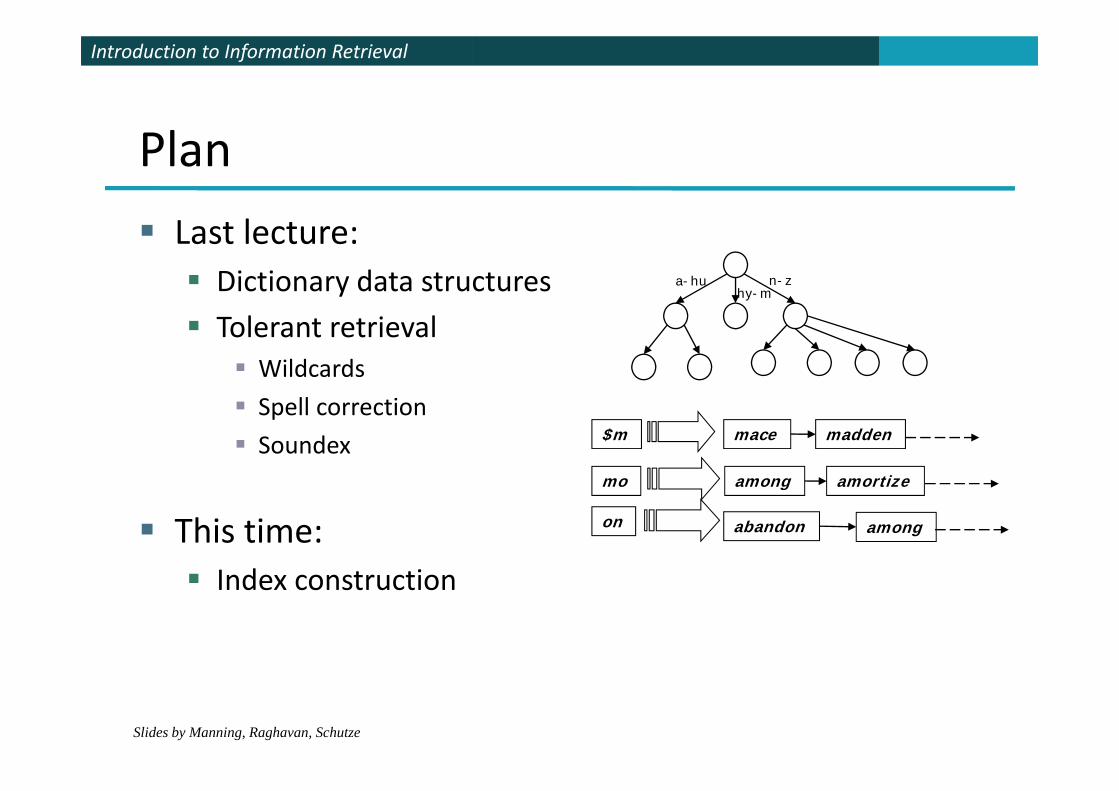
Last lecture: Dictionary data structures a-hu hy-m

n-z

Tolerant retrieval Wildcards

Spell correction

Soundexmo among

$m mace

amortize

madden

This time: Index construction

moon

among

abandon

amortize

among

Index construction


Introduction to Information RetrievalIntroduction to Information Retrieval Ch. 4

Index construction

How do we construct an index?

What strategies can we use with limited main gmemory?


Introduction to Information RetrievalIntroduction to Information Retrieval Sec. 4.1

Hardware basics

Many design decisions in information retrieval are based on the characteristics of hardware

We begin by reviewing hardware basics



Hardware basics

Access to data in memory is much faster than access to data on disk.

Disk seeks: No data is transferred from disk while the disk head is being positioned.

Therefore: Transferring one large chunk of data from disk to memory is faster than transferring many small d s o e o y s as e a a s e g a y s achunks.

Disk I/O is block‐based: Reading and writing of entire Disk I/O is block‐based: Reading and writing of entire blocks (as opposed to smaller chunks).

Block sizes 8KB to 256 KB


Block sizes: 8KB to 256 KB.


Hardware basics

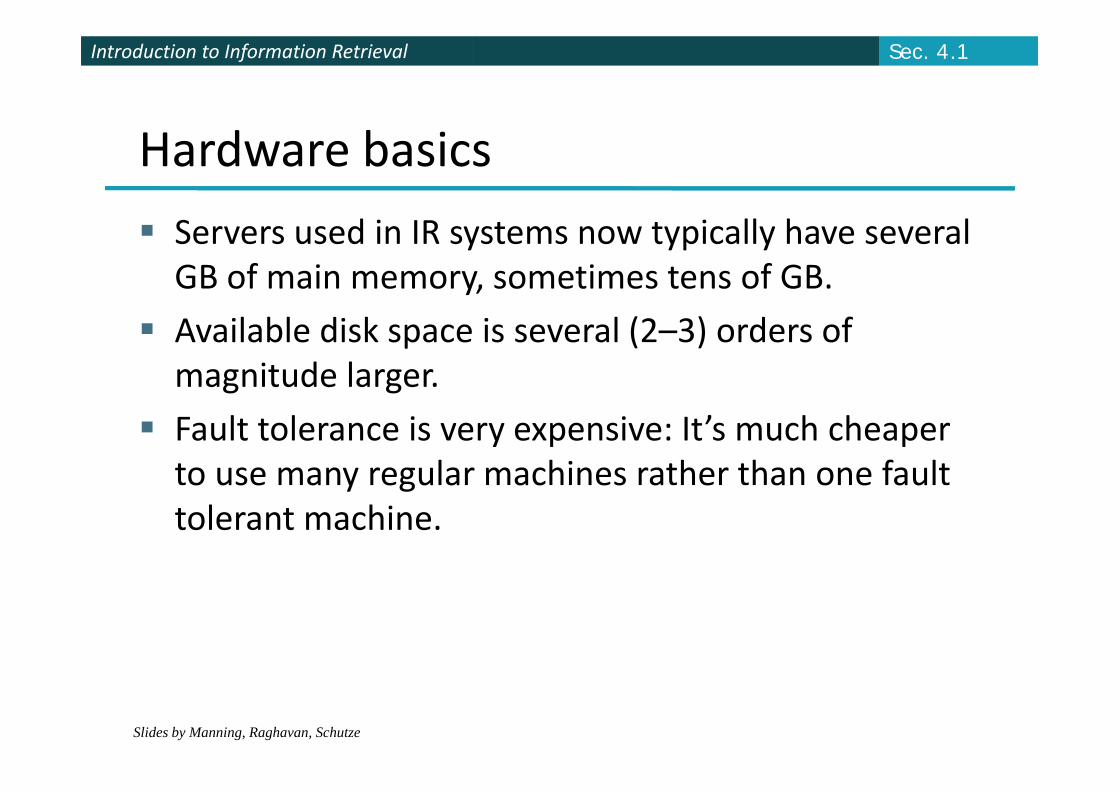
Servers used in IR systems now typically have several GB of main memory, sometimes tens of GB.

Available disk space is several (2–3) orders of magnitude larger.

Fault tolerance is very expensive: It’s much cheaper to use many regular machines rather than one fault o use a y egu a ac es a e a o e autolerant machine.



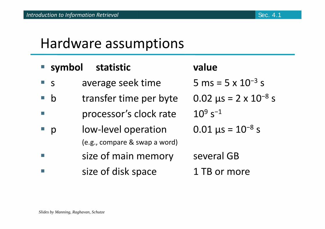
Hardware assumptions

symbol statistic value

s average seek time 5 ms = 5 x 10−3 s

b transfer time per byte 0.02 μs = 2 x 10−8 s

processor’s clock rate 109 s−1 processor s clock rate 10 s

p low‐level operation 0.01 μs = 10−8 s( & d)(e.g., compare & swap a word)

size of main memory several GB

size of disk space 1 TB or more



RCV1: Our collection for this lecture

Shakespeare’s collected works definitely aren’t large enough for demonstrating many of the points in this course.

The collection we’ll use isn’t really large enough either, but it’s publicly available and is at least a more plausible example.

As an example for applying scalable index construction algorithms, we will use the Reuters g ,RCV1 collection.

This is one year of Reuters newswire (part of 1995


This is one year of Reuters newswire (part of 1995 and 1996)


A Reuters RCV1 document


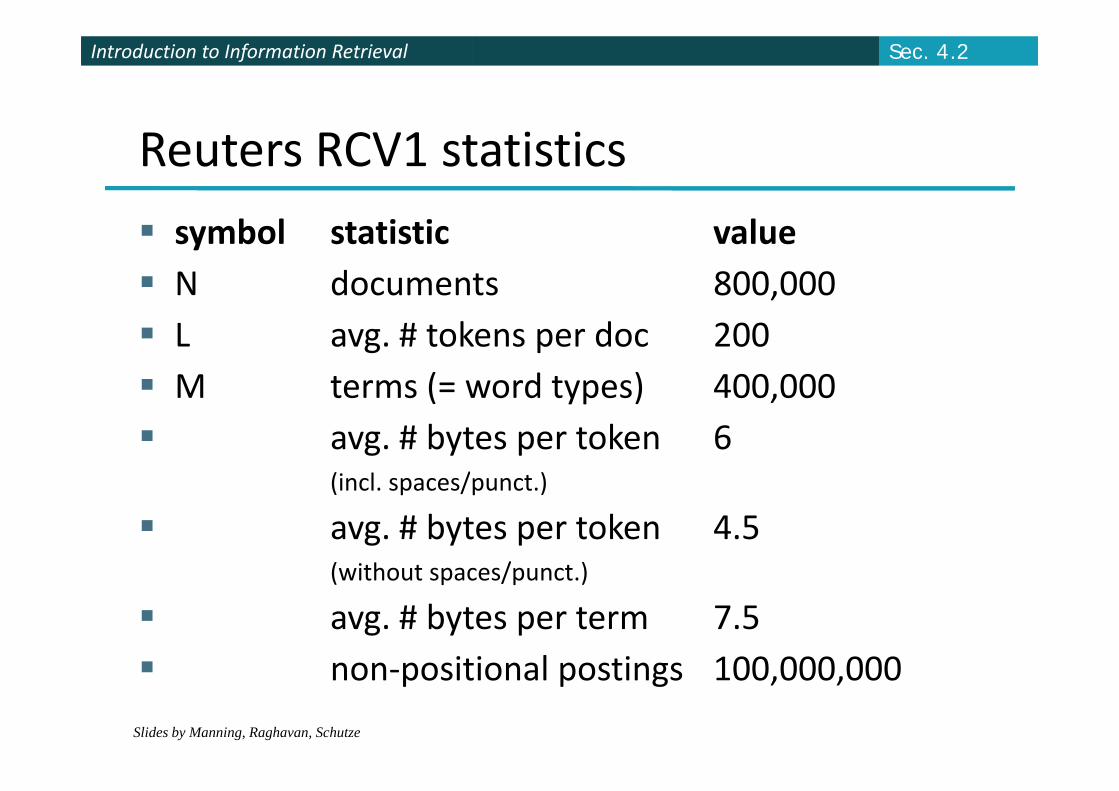
Reuters RCV1 statistics

symbol statistic value N documents 800,000 L avg. # tokens per doc 200 M terms (= word types) 400,000M terms ( word types) 400,000 avg. # bytes per token 6

(incl spaces/punct )(incl. spaces/punct.)

avg. # bytes per token 4.5(without spaces/punct )(without spaces/punct.)

avg. # bytes per term 7.5 non positional postings 100 000 000


non‐positional postings 100,000,000


Term Doc #

Sec. 4.2

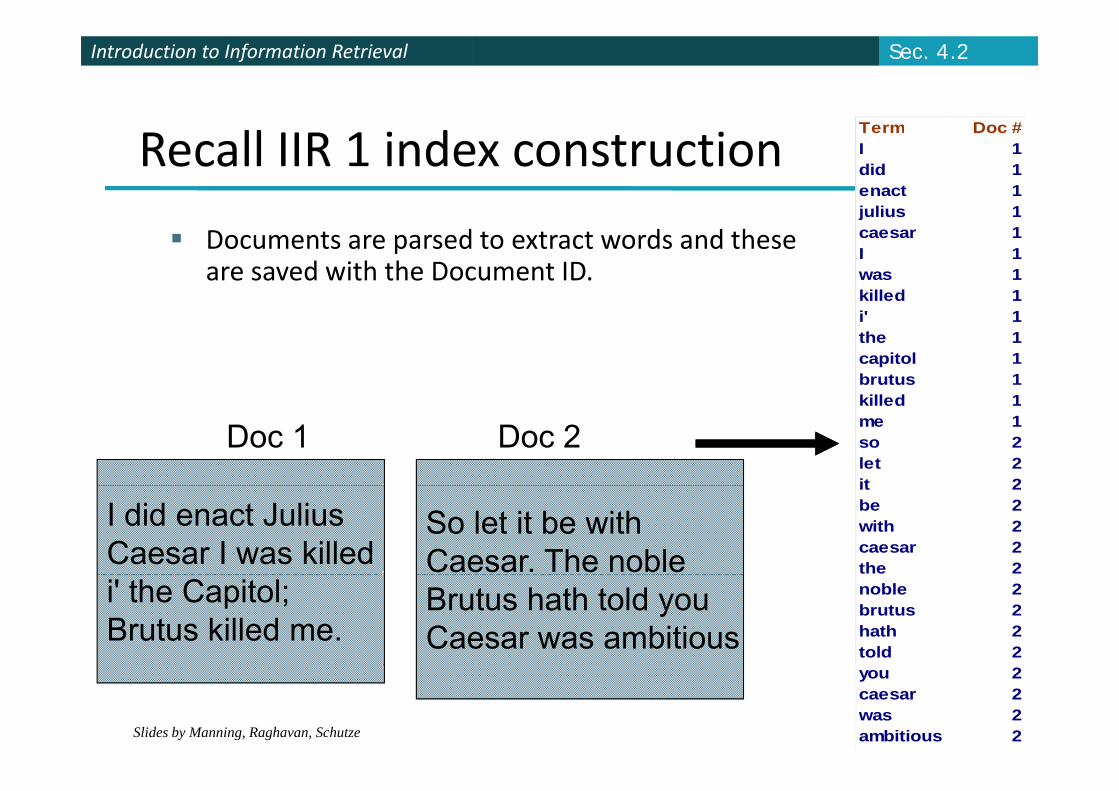
Recall IIR 1 index constructionTerm Doc #I 1did 1enact 1julius 1

Documents are parsed to extract words and these are saved with the Document ID.

julius 1caesar 1I 1was 1killed 1i' 1the 1capitol 1brutus 1kill d 1

Doc 1 Doc 2killed 1me 1so 2let 2it 2

I did enact JuliusCaesar I was killed

So let it be withCaesar. The noble

it 2be 2with 2caesar 2the 2

i' the Capitol; Brutus killed me.

Brutus hath told youCaesar was ambitious

noble 2brutus 2hath 2told 2


you 2caesar 2was 2ambitious 2


Term Doc #I 1did 1enact 1j li 1

Term Doc #ambitious 2be 2brutus 1b t 2

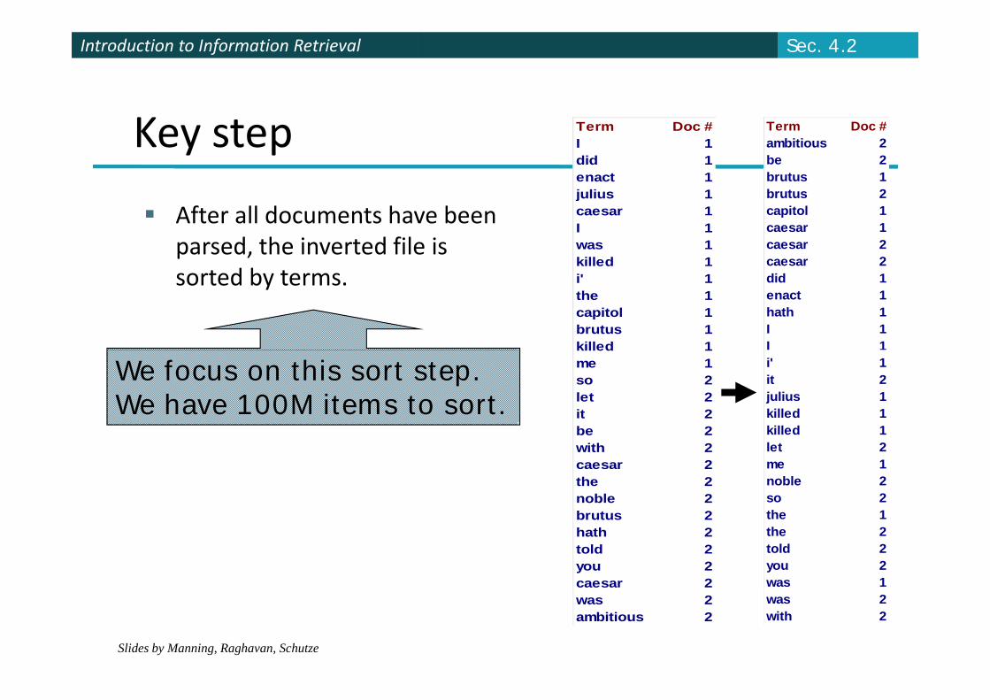
Key stepjulius 1caesar 1I 1was 1killed 1

brutus 2capitol 1caesar 1caesar 2caesar 2

After all documents have been parsed, the inverted file is

t d b t i' 1the 1capitol 1brutus 1killed 1

did 1enact 1hath 1I 1I 1

sorted by terms.

killed 1me 1so 2let 2it 2be 2

i' 1it 2julius 1killed 1killed 1

We focus on this sort step.We have 100M items to sort.

be 2with 2caesar 2the 2noble 2

killed 1let 2me 1noble 2so 2

brutus 2hath 2told 2you 2caesar 2

the 1the 2told 2you 2was 1


was 2ambitious 2

was 2with 2


Scaling index construction

In‐memory index construction does not scale.

How can we construct an index for very large collections?

Taking into account the hardware constraints we justTaking into account the hardware constraints we just learned about . . .

Memory disk speed etc Memory, disk, speed, etc.



Sort‐based index construction As we build the index, we parse docs one at a time.

While building the index, we cannot easily exploit i t i k ( b h l )compression tricks (you can, but much more complex)

The final postings for any term are incomplete until the end.

A 12 b i i l i ( d At 12 bytes per non‐positional postings entry (term, doc, freq), demands a lot of space for large collections.

T 100 000 000 in the case of RCV1 T = 100,000,000 in the case of RCV1

So … we can do this in memory in 2009, but typical collections are much larger E g the New York Timescollections are much larger. E.g. the New York Times provides an index of >150 years of newswire

Thus: We need to store intermediate results on disk.


Thus: We need to store intermediate results on disk.


Use the same algorithm for disk?

Can we use the same index construction algorithm for larger collections, but by using disk instead of memory?

No: Sorting T = 100,000,000 records on disk is too slow – too many disk seeks.

We need an external sorting algorithm.e eed a e e a so g a go



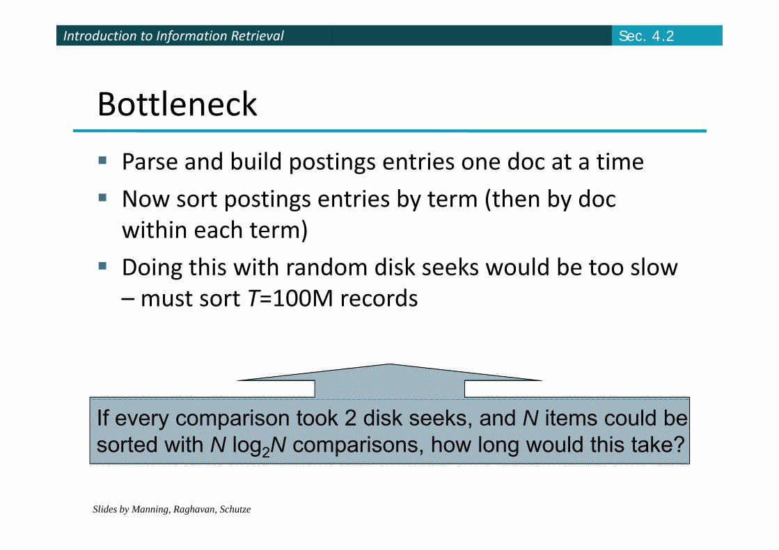
Bottleneck

Parse and build postings entries one doc at a time

Now sort postings entries by term (then by doc within each term)

Doing this with random disk seeks would be too slowDoing this with random disk seeks would be too slow – must sort T=100M records

If every comparison took 2 disk seeks, and N items could besorted with N log2N comparisons, how long would this take?



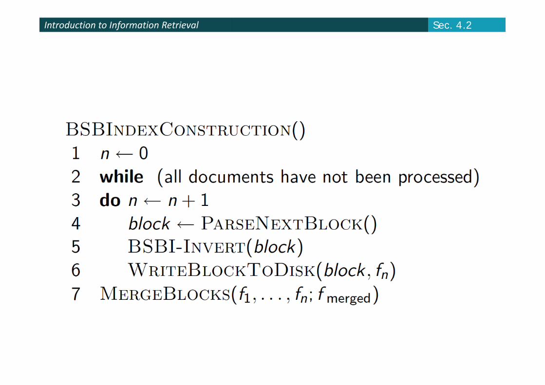
BSBI: Blocked sort‐based Indexing Sec. 4.2

(Sorting with fewer disk seeks)

12‐byte (4+4+4) records (term, doc, freq).

These are generated as we parse docs.

Must now sort 100M such 12‐byte records by term.

Define a Block ~ 10M such records Define a Block 10M such records Can easily fit a couple into memory.

Will have 10 such blocks to start with Will have 10 such blocks to start with.

Basic idea of algorithm: Accumulate postings for each block, sort, write to disk.

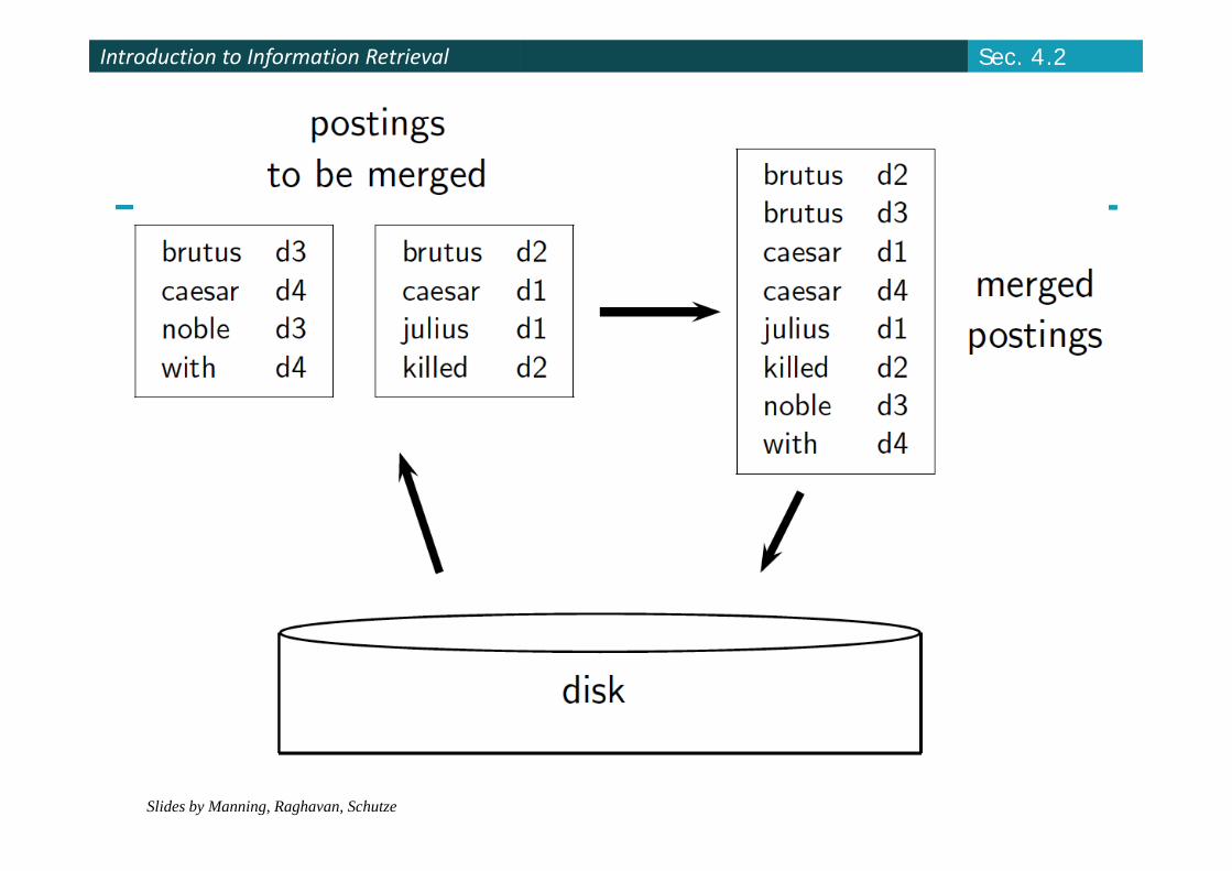
Then merge the blocks into one long sorted order.



Sorting 10 blocks of 10M records

First, read each block and sort within: Quicksort takes 2N ln N expected steps

In our case 2 x (10M ln 10M) steps

Exercise: estimate total time to read each block from Exercise: estimate total time to read each block from ffdisk and disk and quicksortquicksort it.it.

10 times this estimate – gives us 10 sorted runs of10 times this estimate gives us 10 sorted runs of 10M records each.

Done straightforwardly need 2 copies of data on disk Done straightforwardly, need 2 copies of data on disk But can optimize this



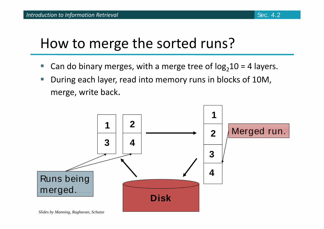
How to merge the sorted runs? Can do binary merges, with a merge tree of log210 = 4 layers.

During each layer, read into memory runs in blocks of 10M, merge, write back.

113 4

2 21

Merged run.3 4

34Runs being

merged.Slides by Manning, Raghavan, Schutze

Diskmerged.


How to merge the sorted runs? But it is more efficient to do a n‐way merge, where you are

reading from all blocks simultaneously

P idi d d t i d h k f h bl k i t Providing you read decent‐sized chunks of each block into memory and then write out a decent‐sized output chunk, then you’re not killed by disk seeksthen you re not killed by disk seeks



Remaining problem with sort‐based Sec. 4.3

algorithm

Our assumption was: we can keep the dictionary in memory.

We need the dictionary (which grows dynamically) in order to implement a term to termID mapping.

Actually, we could work with term,docID postings instead of termID,docID postings . . .s ead o e ,doc pos gs

. . . but then intermediate files become very large. (We would end up with a scalable but very slow(We would end up with a scalable, but very slow index construction method.)



SPIMI: Sec. 4.3

Single‐pass in‐memory indexing

Key idea 1: Generate separate dictionaries for each block – no need to maintain term‐termID mapping across blocks.

Key idea 2: Don’t sort. Accumulate postings in postings lists as they occur.

With these two ideas we can generate a complete ese o deas e ca ge e a e a co p e einverted index for each block.

These separate indexes can then be merged into one These separate indexes can then be merged into one big index.



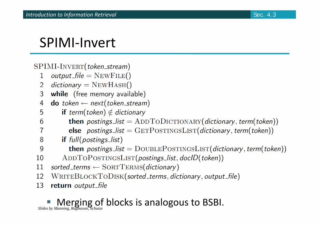
SPIMI‐Invert

Slides by Manning, Raghavan, Schutze Merging of blocks is analogous to BSBI.


SPIMI: Compression

Compression makes SPIMI even more efficient. Compression of terms

Compression of postings

See next lecture



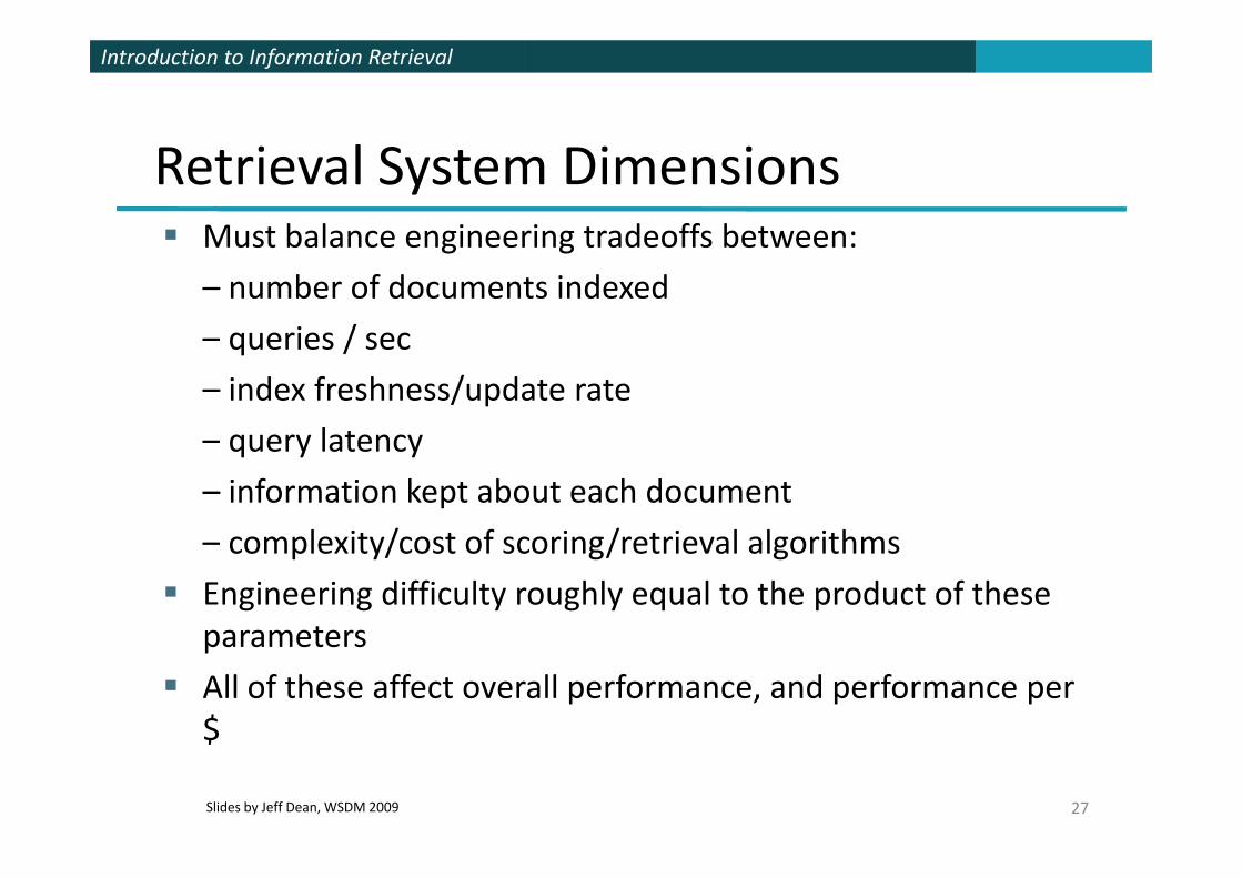
Retrieval System Dimensions Must balance engineering tradeoffs between:Must balance engineering tradeoffs between:

– number of documents indexed

– queries / sec– queries / sec

– index freshness/update rate

query latency– query latency

– information kept about each document

complexity/cost of scoring/retrieval algorithms– complexity/cost of scoring/retrieval algorithms

Engineering difficulty roughly equal to the product of these parametersparameters

All of these affect overall performance, and performance per $


$

27Slides by Jeff Dean, WSDM 2009


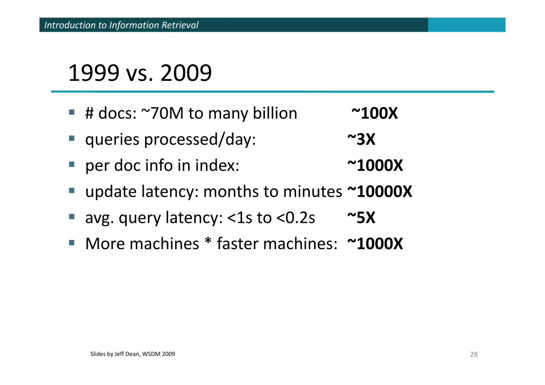
1999 vs. 2009

# docs: ~70M to many billion ~100X

queries processed/day: ~3X

per doc info in index: ~1000X

update latency: months to minutes ~10000X update latency: months to minutes 10000X

avg. query latency: <1s to <0.2s ~5X

More machines * faster machines: ~1000X

Slides by Manning, Raghavan, Schutze 28Slides by Jeff Dean, WSDM 2009


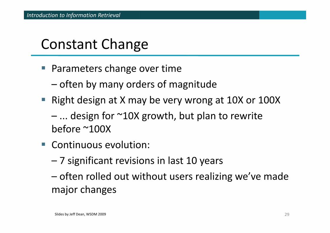
Constant Change

Parameters change over time

– often by many orders of magnitude

Right design at X may be very wrong at 10X or 100X

– design for ~10X growth but plan to rewrite– ... design for 10X growth, but plan to rewrite before ~100X

Contin o s e ol tion Continuous evolution:

– 7 significant revisions in last 10 years

– often rolled out without users realizing we’ve made major changes



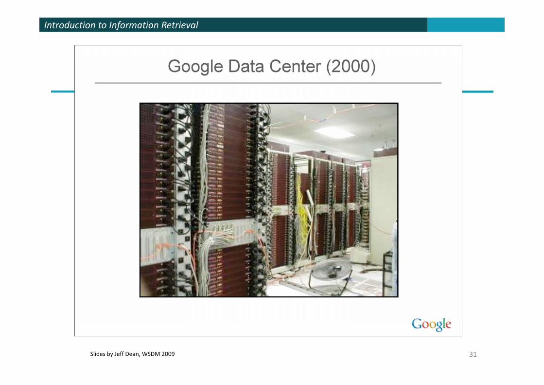
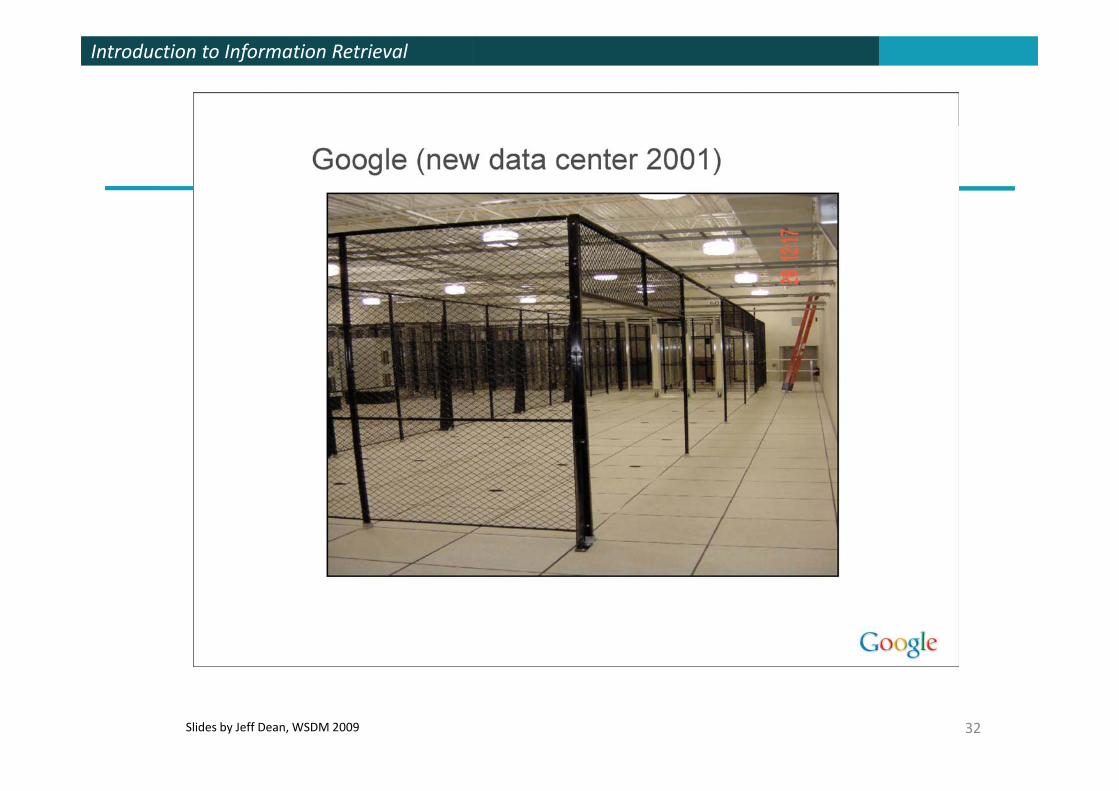
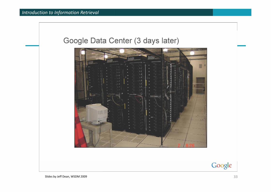
Google data centers

Google data centers mainly contain commodity machines.

Data centers are distributed around the world.

Estimate: a total of 1 million servers, 3 millionEstimate: a total of 1 million servers, 3 million processors/cores (Gartner 2007)

Estimate: Google installs 100 000 servers each Estimate: Google installs 100,000 servers each quarter. Based on expenditures of 200 250 million dollars per year Based on expenditures of 200–250 million dollars per year

This would be 10% of the computing capacity of the ld!?!


world!?!


Google data centers

If in a non‐fault‐tolerant system with 1000 nodes, each node has 99.9% uptime, what is the uptime of the system?

Answer: 63%

Calculate the number of servers failing per minute for an installation of 1 million servers.o a s a a o o o se e s



Distributed indexing

Maintain a mastermachine directing the indexing job – considered “safe”.

Break up indexing into sets of (parallel) tasks.

Master machine assigns each task to an idle machineMaster machine assigns each task to an idle machine from a pool.



Parallel tasks

We will use two sets of parallel tasks Parsers

Inverters

Break the input document collection into splitsp p

Each split is a subset of documents (corresponding to blocks in BSBI/SPIMI)blocks in BSBI/SPIMI)



Parsers

Master assigns a split to an idle parser machine

Parser reads a document at a time and emits (term, doc) pairs

Parser writes pairs into j partitionsParser writes pairs into j partitions

Each partition is for a range of terms’ first letters (e g a f g p q z) here j = 3 (e.g., a‐f, g‐p, q‐z) – here j = 3.

Now to complete the index inversion



Inverters

An inverter collects all (term,doc) pairs (= postings) for one term‐partition.

Sorts and writes to postings lists



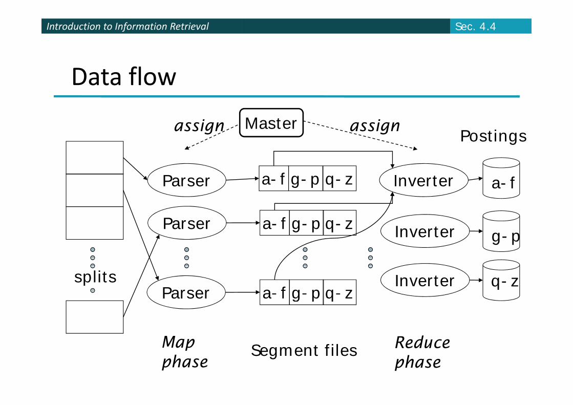
Data flow

Master Postingsassign assign

Parser a-f g-p q-z Inverter a-f

Parser a-f g-p q-z Inverter g-p

splitsParser a-f g-p q-z Inverter q-zParser a f g p q z

Map ReduceMapphase

Segment files Reducephase


MapReduce

The index construction algorithm we just described is an instance of MapReduce.

MapReduce (Dean and Ghemawat 2004) is a robust and conceptually simple framework for distributed computing …

… without having to write code for the distribution ou a g o e code o e d s bu opart.

They describe the Google indexing system (ca 2002) They describe the Google indexing system (ca. 2002) as consisting of a number of phases, each implemented in MapReduce


implemented in MapReduce.


MapReduce

Index construction was just one phase.

Another phase: transforming a term‐partitioned index into a document‐partitioned index. Term‐partitioned: one machine handles a subrange of terms

Document‐partitioned: one machine handles a subrange of documents

As we discuss in the web part of the course) most search engines use a document‐partitioned index … better load balancing, etc.



Schema for index construction in Sec. 4.4

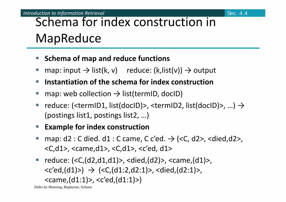
MapReduce Schema of map and reduce functions

map: input → list(k, v) reduce: (k,list(v)) → output

Instantiation of the schema for index construction

map: web collection → list(termID, docID)

reduce: (<termID1, list(docID)>, <termID2, list(docID)>, …) → (postings list1, postings list2, …)

l f d Example for index construction

map: d2 : C died. d1 : C came, C c’ed. → (<C, d2>, <died,d2>, <C d1> < d1> <C d1> < ’ d d1><C,d1>, <came,d1>, <C,d1>, <c’ed, d1>

reduce: (<C,(d2,d1,d1)>, <died,(d2)>, <came,(d1)>, <c’ed (d1)>) → (<C (d1:2 d2:1)> <died (d2:1)>


<c ed,(d1)>) → (<C,(d1:2,d2:1)>, <died,(d2:1)>, <came,(d1:1)>, <c’ed,(d1:1)>)


Dynamic indexing

Up to now, we have assumed that collections are static.

They rarely are: Documents come in over time and need to be inserted.

Documents are deleted and modified.

This means that the dictionary and postings lists haveThis means that the dictionary and postings lists have to be modified: Postings updates for terms already in dictionaryPostings updates for terms already in dictionary

New terms added to dictionary



Simplest approach

Maintain “big” main index

New docs go into “small” auxiliary index

Search across both, merge results

Deletions Deletions Invalidation bit‐vector for deleted docs

Filter docs output on a search result by this invalidation Filter docs output on a search result by this invalidation bit‐vector

Periodically re index into one main index Periodically, re‐index into one main index



Issues with main and auxiliary indexes Problem of frequent merges – you touch stuff a lot

Poor performance during merge

Actually: Merging of the auxiliary index into the main index is efficient if we

keep a separate file for each postings listkeep a separate file for each postings list.

Merge is the same as a simple append.

But then we would need a lot of files – inefficient for O/S.

Assumption for the rest of the lecture: The index is one big file.

In reality: Use a scheme somewhere in between (e.g., split very large postings lists, collect postings lists of length 1 in one fil )


file etc.)


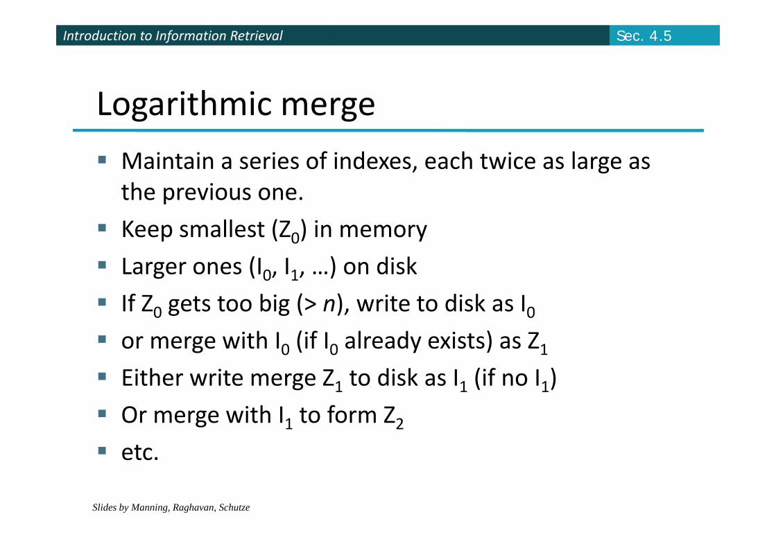
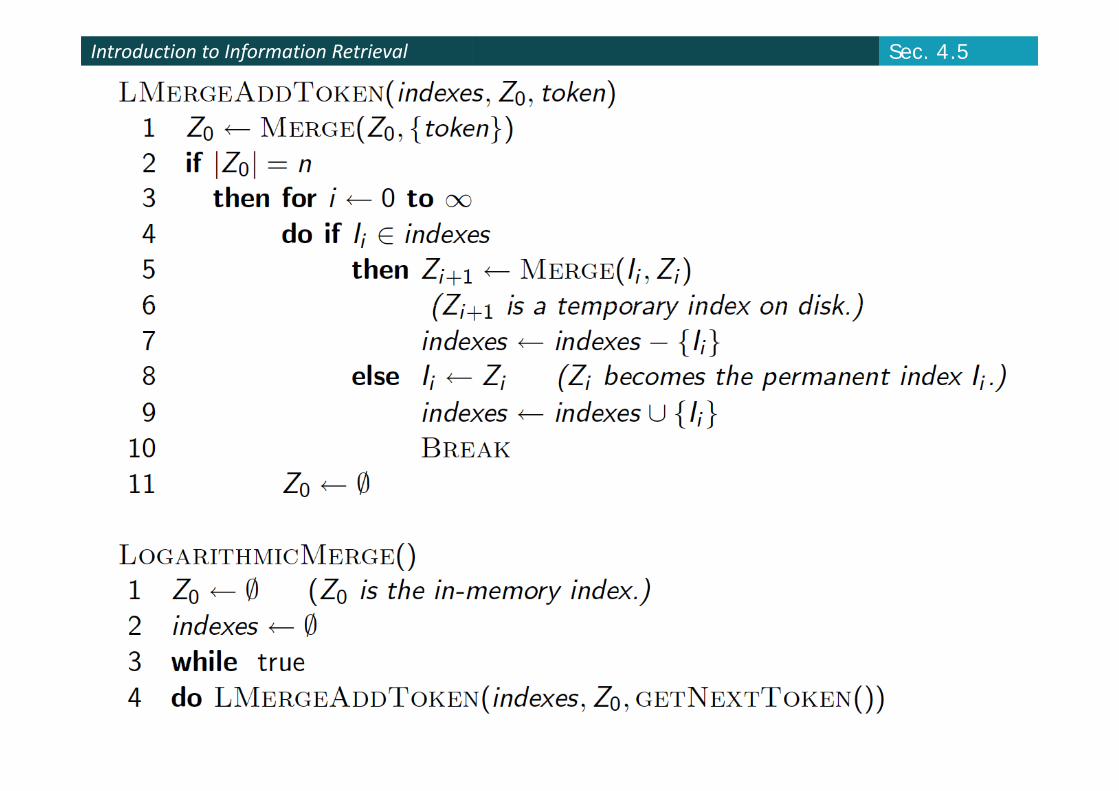
Logarithmic merge

Maintain a series of indexes, each twice as large as the previous one.

Keep smallest (Z0) in memory

Larger ones (I0, I1, …) on diskLarger ones (I0, I1, …) on disk

If Z0 gets too big (> n), write to disk as I0 or merge ith I (if I alread e ists) as Z or merge with I0 (if I0 already exists) as Z1 Either write merge Z1 to disk as I1 (if no I1)

Or merge with I1 to form Z2 etc.



Logarithmic merge

Auxiliary and main index: index construction time is O(T2) as each posting is touched in each merge.

Logarithmic merge: Each posting is merged O(log T) times, so complexity is O(T log T)

So logarithmic merge is much more efficient for index constructionde co s uc o

But query processing now requires the merging of O(log T) indexesO(log T) indexes Whereas it is O(1) if you just have a main and auxiliary index


index


Further issues with multiple indexes

Collection‐wide statistics are hard to maintain

E.g., when we spoke of spell‐correction: which of several corrected alternatives do we present to the user? We said, pick the one with the most hits

How do we maintain the top ones with multipleHow do we maintain the top ones with multiple indexes and invalidation bit vectors? One possibility: ignore everything but the main index forOne possibility: ignore everything but the main index for such ordering

Will see more such statistics used in results ranking


Will see more such statistics used in results ranking


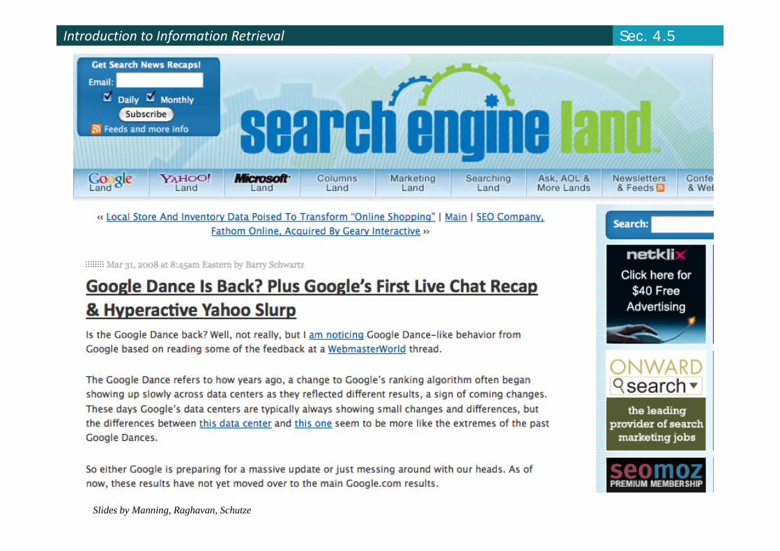
Dynamic indexing at search engines

All the large search engines now do dynamic indexing

Their indices have frequent incremental changes News items, blogs, new topical web pages

Sarah Palin, …

But (sometimes/typically) they also periodically ( yp y) y p yreconstruct the index from scratch Query processing is then switched to the new index, and y p g ,the old index is then deleted



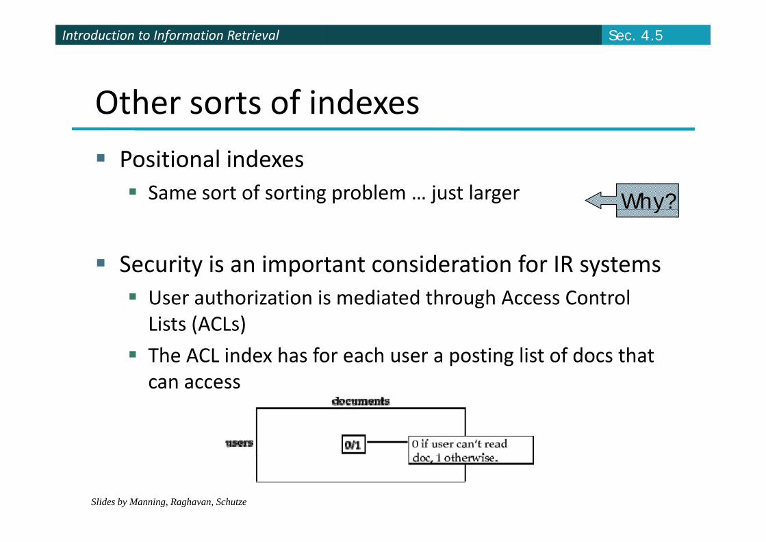
Other sorts of indexes

Positional indexes Same sort of sorting problem … just larger Why?

Security is an important consideration for IR systems

y

Security is an important consideration for IR systems User authorization is mediated through Access Control Lists (ACLs)( )

The ACL index has for each user a posting list of docs that can access


Introduction to Information RetrievalIntroduction to Information Retrieval Ch. 4

Resources for today’s lecture

Chapter 4 of IIR

MG Chapter 5

Original publication on MapReduce: Dean and Ghemawat (2004)Ghemawat (2004)

Original publication on SPIMI: Heinz and Zobel (2003)


Introduction to Information Retrieval ΕΠΛ660 · 2011-02-08 · Introduction to Information...

Documents

Transcript of Introduction to Information Retrieval ΕΠΛ660 · 2011-02-08 · Introduction to Information...