Regular Paper

Probabilistic Coverage Methods inPeople-Centric Sensing

Abstract

To achieve sensing coverage for a given Areas of Interest (AoI) over time at low

cost in a People-Centric Sensing manner, we propose a concept of (α, T )-coverage of

a target field where each point in the field is sensed by at least one mobile node with

probability of at least α during time period T . Our goal is to achieve (α, T )-coverage

of a given AoI by a minimal set of mobile nodes. In this paper, we propose two algo-

rithms: inter-location algorithm that selects a minimal number of mobile nodes from

nodes inside the AoI considering the distance between them and inter-meeting-time

algorithm that selects nodes regarding the expected meeting time between the nodes.

To cope with the case that there is insufficient number of nodes inside AoI, we pro-

pose an extended algorithm which regards nodes inside and outside AoI. To improve

the accuracy of the proposed algorithms, we also propose an updating mechanism

which adapts the number of selected nodes based on their latest locations during

the time period T . In our simulation-based performance evaluation, our algorithms

achieved (α, T )-coverage with good accuracy for various values of α, T , AoI size,

and moving probability.

i

1. Introduction

Recently, the demand for realtime environmental information about specific re-

gions in urban areas has been increasing for various purposes such as surveillance,

navigation, and event detection. People moving inside an urban area give the pos-

sibility to cover a given area of interest (AoI) at low cost. Exploiting people as a

part of the sensing infrastructure, introduces a new sensing paradigm called People-

Centric Sensing (PCS)1). PCS realizes that people with mobile devices can act as

mobile sensors to sense and gather information from the environment to serve sens-

ing applications and their users. In PCS, the coverage depends on the uncontrollable

mobility of people, therefore it is difficult to achieve the full coverage of the target

AoI. Consequently, it is preferable to measure the expected coverage degree as a

ratio.

Here, we describe our motivation scenario and our problem settings. The realtime

urban sensing scenarios drive an interesting motivating application. In a city sensing

application, for instance, users want to know the information in a specific AoI such

as interesting spots, crowded places, events on specific locations, and so on. In such

an application, a user sends a query about a geographic area as the AoI, a required

coverage ratio α (i.e., the required percent of coverage of the AoI), the required

information (e.g., noise level), and a query interval (maximum allowable response

time) T . Then, the query responding process will be carried out by some people with

mobile devices in the AoI, which satisfy the query requirements. Here, to minimize

cost, it is desirable to select a minimal number of people with mobile devices that

can provide the desired information. We refer to this problem as the (α, T )-coverage

problem.

In this paper, we formally describe the (α, T )-coverage problem. Given a target

field that is composed of a set of points, an AoI as a subset of it, a set of mobile

nodes, and a query with a required coverage ratio α and a specified time interval T ,

we define the problem that finds a minimal set of mobile nodes such that each point

in the AoI is visited and sensed by at least one node within T with a probability of

at least α. To solve this problem, we need to predict the future locations visited by

each mobile node depending on its current location when a query is initiated and its

1

mobility. Thus, we model the mobility of the mobile nodes with a discrete Markov

chain. The solution for this problem depends critically on the number and the ini-

tial locations of mobile nodes inside and near the target AoI. One possible solution

for this problem is random selection of nodes. The main drawback of the random

selection is inefficiency by selecting a set of nodes that are likely to visit the same lo-

cations in AoI in the future and this set may not be minimal to achieve the coverage.

To avoid this drawback, we should carefully select a minimal set of nodes that are not

likely to visit the same locations. Based on this insight, we propose two algorithms:

inter-location and inter-meeting-time algorithms, to meet a coverage ratio α in time

period T . The inter-location algorithm estimates the probability of locations in the

AoI being visited by each mobile sensor node in T , and selects a minimal number of

mobile nodes inside the AoI considering the distance between the nodes. The inter-

meeting-time algorithm selects a minimal number of nodes regarding the expected

time until any two of the nodes will meet at a location. Sometimes, the required cov-

erage may not be achieved due to insufficient number of nodes existing inside AoI.

To meet the required coverage in this case, we also propose an extended algorithm

which takes into account not only nodes existing inside AoI, but also nodes outside

AoI.

Future estimated location of each node could be inaccurate when T is large, re-

sulting in inaccurate coverage. For more accurate coverage, we propose an updating

mechanism for the inter-location and the inter-meeting-time algorithms which aims

to remove useless nodes and add some extra nodes that contribute more to AoI cover-

age. This updating mechanism is periodically executed every specified time interval

during T .

We conducted simulation experiments to evaluate the performance of the proposed

algorithms for various parameter settings. As a result, we confirmed that the pro-

posed algorithms achieve (α, T )-coverage with good accuracy for a variety of val-

ues of α, T , and AoI size, and the inter-meeting time algorithm selected the smallest

number of nodes without deteriorating coverage accuracy.

The rest of this paper is organized as follows. Section 2 reviews the related studies.

Section 3 defines the (α, T )-coverage problem. Section 4 describes the proposed

algorithms. Section 5 shows the performance evaluation of the proposed algorithms

2

through simulation-based experiments, and finally Section 6 concludes the paper.

2. Related Work

Many studies have proposed data gathering protocols to realize efficient communi-

cation between sensor nodes in wireless sensor networks (WSNs)2)–5). Some studies

also have proposed to use mobile sensor nodes in WSNs to improve coverage, life-

time, and/or fault-tolerance6),7).

Recently, information collection by pedestrians in PCS has received increasing

attentions. PCS is different from existing WSNs because we cannot control the mo-

bility of mobile nodes. In addition, the two important criteria in PCS are coverage of

the AoI and time. There are several studies and research projects based on PCS8)–15).

Cartel8) is a mobile communications infrastructure based on car-mounted commu-

nication platforms exploiting open WiFi access points in a city, and provides urban

sensing information such as traffic conditions. CitySense9) provides a static sensor

mesh offering similar types of urban sensing data feeds. SensorPlanet10) is a plat-

form that enables the collection of sensor data on a large and heterogeneous scale,

and establishes a central repository for sharing the collected sensor data. Bubble-

sensing11) is a sensor network that allows mobile phone users to create a binding

between tasks and places of interest in the physical world. Mobile users are able

to affix task bubbles at places of interest and then receive sensed data as it becomes

available in a delay-tolerant fashion. PriSense12) relies on data slicing and mixing and

binary search to enable privacy-preserving queries, where each node slices its data

into (n + 1) data slices, randomly chooses n other nodes, and sends a unique data

slice to each of them. Finally, each node sends the sum of its own slice and the slices

received from others to the aggregation server. Anonysense13) is a privacy-aware ar-

chitecture for realizing pervasive applications based on collaborative, opportunistic

sensing by personal mobile devices. AnonySense allows applications to query and

receive context through an expressive task language and by leveraging a broad range

of sensor types on mobile devices, and at the same time respects the privacy of users.

GreenGPS15) is a navigation service that uses participatory sensing data to map fuel

consumption on city streets and find the most fuel-efficient route for vehicles between

arbitrary endpoints.

3

Most of these approaches focus on information collection, but do not consider the

probabilistic coverage in PCS when the information collection period is restricted to

a short time duration such as an on-demand query. They consider neither the difficul-

ties to achieve sensing coverage of a relatively wide area nor the time requirements of

on-demand sensing by mobile users. However, these two criteria are very important

in PCS. To meet these criteria, it is also very important to estimate the area covered

by each mobile node in a specified time interval. However, existing studies do not

consider such a spatiotemporal coverage by mobile nodes.

In 16) and 17), we formulated the (α, T )-coverage problem and proposed two

probabilistic algorithms: inter-location based algorithm, called ILB, and inter-meeting-

time based algorithm, called IMTB, that consider on-demand sensing by mobile

users, and probabilistic coverage in PCS based on the mobility of people. Also,

we evaluated the performance of ILB and IMTB for various parameter settings in-

cluding a realistic scenario on a specific city map. ILB and IMTB algorithms were

based only on the initial locations of mobile nodes inside AoI and did not consider

the latest locations during the time period. To improve the accuracy of the proposed

algorithms, our contribution in this paper is the proposal of two extensions: (i) an

updating mechanism for ILB and IMTB algorithms which aims to remove useless

nodes and add some extra nodes that contribute more to AoI coverage during query

interval, and (ii) an extended algorithm which regards not only nodes existing inside

AoI, but also nodes near AoI. In addition, we compare the proposed algorithms with

a random selection method to evaluate their performance.

3. The (α, T )-Coverage Problem

In this section, we first describe the models and assumptions for our target PCS

application, then formulate the target problem to realize the application.

3.1 Assumptions and Models

3.1.1 System Model

We assume an application such that when requested, some of the mobile users take

part in a task to obtain the latest environmental information such as noise level, sun-

shine intensity, temperature, exhaust gas concentration, and so on, over a specified

4

geographical area of the urban district in a PCS fashion. We assume that those par-

ticipating users are collaborative to serve as mobile sensors based on some incentive

such as electronic currency or coupons given by a service provider.

We denote the whole service area by A. A road (street) network on which mobile

users can move spans the area A. A service user wants to know the approximate con-

dition of a specific area called the Area of Interest (AoI) produced by obtaining the

environmental information about some locations in the AoI. Thus, we assume that

there are multiple sensing locations with a uniform spacing ∆⋆1 (e.g., ∆ = 50m)

on each road and that sensing coverage is achieved by obtaining the environmen-

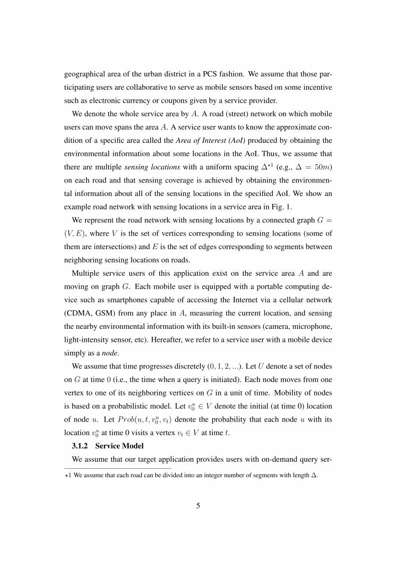
tal information about all of the sensing locations in the specified AoI. We show an

example road network with sensing locations in a service area in Fig. 1.

We represent the road network with sensing locations by a connected graph G =

(V,E), where V is the set of vertices corresponding to sensing locations (some of

them are intersections) and E is the set of edges corresponding to segments between

neighboring sensing locations on roads.

Multiple service users of this application exist on the service area A and are

moving on graph G. Each mobile user is equipped with a portable computing de-

vice such as smartphones capable of accessing the Internet via a cellular network

(CDMA, GSM) from any place in A, measuring the current location, and sensing

the nearby environmental information with its built-in sensors (camera, microphone,

light-intensity sensor, etc). Hereafter, we refer to a service user with a mobile device

simply as a node.

We assume that time progresses discretely (0, 1, 2, ...). Let U denote a set of nodes

on G at time 0 (i.e., the time when a query is initiated). Each node moves from one

vertex to one of its neighboring vertices on G in a unit of time. Mobility of nodes

is based on a probabilistic model. Let vu0 ∈ V denote the initial (at time 0) location

of node u. Let Prob(u, t, vu0 , vt) denote the probability that each node u with its

location vu0 at time 0 visits a vertex vt ∈ V at time t.

3.1.2 Service Model

We assume that our target application provides users with on-demand query ser-

⋆1 We assume that each road can be divided into an integer number of segments with length ∆.

5

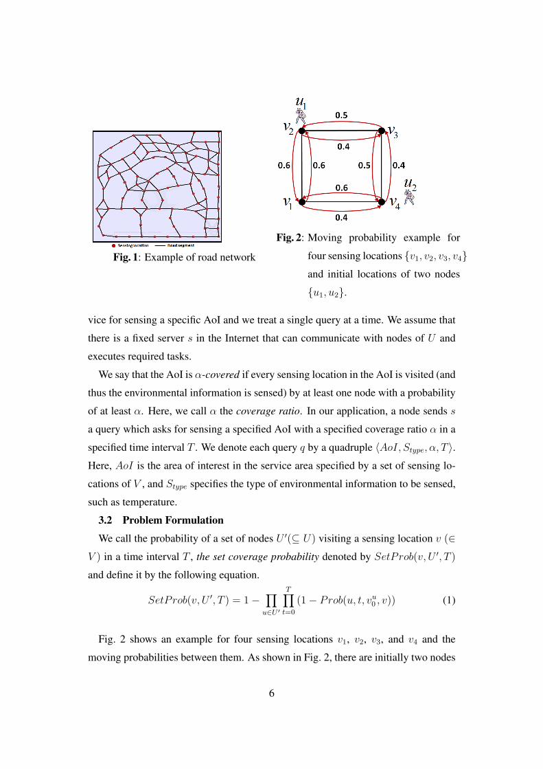
Fig. 1: Example of road network

Fig. 2: Moving probability example for

four sensing locations {v1, v2, v3, v4}and initial locations of two nodes

{u1, u2}.

vice for sensing a specific AoI and we treat a single query at a time. We assume that

there is a fixed server s in the Internet that can communicate with nodes of U and

executes required tasks.

We say that the AoI is α-covered if every sensing location in the AoI is visited (and

thus the environmental information is sensed) by at least one node with a probability

of at least α. Here, we call α the coverage ratio. In our application, a node sends s

a query which asks for sensing a specified AoI with a specified coverage ratio α in a

specified time interval T . We denote each query q by a quadruple ⟨AoI, Stype, α, T ⟩.Here, AoI is the area of interest in the service area specified by a set of sensing lo-

cations of V , and Stype specifies the type of environmental information to be sensed,

such as temperature.

3.2 Problem Formulation

We call the probability of a set of nodes U ′(⊆ U) visiting a sensing location v (∈V ) in a time interval T , the set coverage probability denoted by SetProb(v, U ′, T )

and define it by the following equation.

SetProb(v, U ′, T ) = 1−∏u∈U ′

T∏t=0

(1− Prob(u, t, vu0 , v)) (1)

Fig. 2 shows an example for four sensing locations v1, v2, v3, and v4 and the

moving probabilities between them. As shown in Fig. 2, there are initially two nodes

6

Sensing node u1 node u2

location Prob(u1, t, v2, v) Prob(u2, t, v4, v) SetProb(v, U ′, 2)

v t = 0 t = 1 t = 2 t = 0 t = 1 t = 2 U ′ = {u1, u2}

v1 0 0.6 0 0 0.6 0 1− (1− 0.6)(1− 0.6) = 0.84

v2 1 0 0.56 0 0 0.56 1− (1− 1)(1− 0.56)(1− 0.56) = 1

v3 0 0.4 0 0 0.4 0 1− (1− 0.4)(1− 0.4) = 0.64

v4 0 0 0.44 1 0 0.44 1− (1− 0.44)(1− 1)(1− 0.44) = 1

Table 1: Visiting time and set coverage probabilities for the example in Fig. 2 with

T = 2.

u1 and u2 at sensing locations v2 and v4, respectively. Table 1 shows the set coverage

probabilities of v1, v2, v3, and v4 by U ′ = {u1, u2} when T = 2.

Definition 1. (α, T )-coverage: Given a graph G = (V,E), an area specified by a

set of sensing locations AoI ⊆ V , a set of nodes U ′ ⊆ U , a required coverage ratio

α, and a time interval T , the area AoI is called (α, T )-covered if the following

condition holds.

∀v ∈ AoI, SetProb(v, U ′, T ) ≥ α (2)

We formally define the (α, T )-coverage problem as follows:

Definition 2. Given a service area as a connected graph G = (V,E), a set of nodes

U on G at time 0, and a query q = ⟨AoI, Stype, α, T ⟩, the (α, T )-coverage problem

is the problem of selecting a minimal set of nodes U ′ ⊆ U which achieves (α, T )-

coverage of AoI .

We define the objective function of this problem by the following equation.

minimize |U ′| (3)

subject to AoI is (α, T )-covered (4)

This problem is NP-hard since it implies, as a special case, the Minimum Set Cov-

ering Problem (MSCP)18) which is known to be NP-hard.

4. Algorithms

In this section, we propose two heuristic algorithms for the problem defined in

Section 3, named Inter-Location Based (ILB) and Inter-Meeting Time Based (IMTB)

7

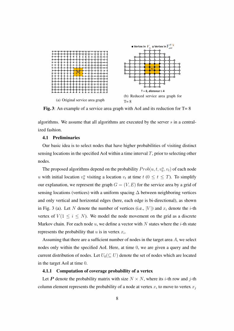
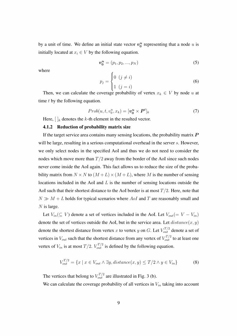
(a) Original service area graph(b) Reduced service area graph forT= 8

Fig. 3: An example of a service area graph with AoI and its reduction for T= 8

algorithms. We assume that all algorithms are executed by the server s in a central-

ized fashion.

4.1 Preliminaries

Our basic idea is to select nodes that have higher probabilities of visiting distinct

sensing locations in the specified AoI within a time interval T , prior to selecting other

nodes.

The proposed algorithms depend on the probability Prob(u, t, vu0 , vt) of each node

u with initial location vu0 visiting a location vt at time t (0 ≤ t ≤ T ). To simplify

our explanation, we represent the graph G = (V,E) for the service area by a grid of

sensing locations (vertices) with a uniform spacing ∆ between neighboring vertices

and only vertical and horizontal edges (here, each edge is bi-directional), as shown

in Fig. 3 (a). Let N denote the number of vertices (i.e., |V |) and xi denote the i-th

vertex of V (1 ≤ i ≤ N ). We model the node movement on the grid as a discrete

Markov chain. For each node u, we define a vector with N states where the i-th state

represents the probability that u is in vertex xi.

Assuming that there are a sufficient number of nodes in the target area A, we select

nodes only within the specified AoI. Here, at time 0, we are given a query and the

current distribution of nodes. Let U0(⊆ U) denote the set of nodes which are located

in the target AoI at time 0.

4.1.1 Computation of coverage probability of a vertex

Let P denote the probability matrix with size N ×N , where its i-th row and j-th

column element represents the probability of a node at vertex xi to move to vertex xj

8

by a unit of time. We define an initial state vector vu0 representing that a node u is

initially located at xi ∈ V by the following equation.

vu0 = (p1, p2, ..., pN) (5)

where

pj =

0 (j ̸= i)

1 (j = i)(6)

Then, we can calculate the coverage probability of vertex xk ∈ V by node u at

time t by the following equation.

Prob(u, t, vu0 , xk) = [vu0 × P t]k (7)

Here, [ ]k denotes the k-th element in the resulted vector.

4.1.2 Reduction of probability matrix size

If the target service area contains many sensing locations, the probability matrix P

will be large, resulting in a serious computational overhead in the server s. However,

we only select nodes in the specified AoI and thus we do not need to consider the

nodes which move more than T/2 away from the border of the AoI since such nodes

never come inside the AoI again. This fact allows us to reduce the size of the proba-

bility matrix from N ×N to (M +L)× (M +L), where M is the number of sensing

locations included in the AoI and L is the number of sensing locations outside the

AoI such that their shortest distance to the AoI border is at most T/2. Here, note that

N ≫M + L holds for typical scenarios where AoI and T are reasonably small and

N is large.

Let Vin(⊆ V ) denote a set of vertices included in the AoI. Let Vout(= V − Vin)

denote the set of vertices outside the AoI, but in the service area. Let distance(x, y)

denote the shortest distance from vertex x to vertex y on G. Let V T/2out denote a set of

vertices in Vout such that the shortest distance from any vertex of V T/2out to at least one

vertex of Vin is at most T/2. V T/2out is defined by the following equation.

VT/2out = {x | x ∈ Vout ∧ ∃y, distance(x, y) ≤ T/2 ∧ y ∈ Vin} (8)

The vertices that belong to VT/2out are illustrated in Fig. 3 (b).

We can calculate the coverage probability of all vertices in Vin taking into account

9

only the node moving probability at each vertex of Vin ∪ VT/2out . Consequently, we

define the new probability matrix P ′ for vertices of Vin ∪ VT/2out .

We define the i-th row and j-th column element p′i,j of P ′ by the following equa-

tion.

p′i,j =

pi,j (xi, xj ∈ Vin ∪ VT/2out ∧ i ̸= j)

∑x∈Ngh(i)

p(i, x) (xi ∈ VT/2out − V

T/2−1out ∧ i = j)

(9)

Here, Ngh(i) is the set of neighboring vertices outside VT/2out and pi,j is the prob-

ability of the corresponding edge in the original matrix P . Equation (9) represents

that the moving probability from xi to xj is the same as the original matrix P if i is

not equal to j. In addition, knowing that nodes once going outside VT/2out cannot go

inside AoI in T , we for convenience set the probability of a node staying at the same

location xi at border of V T/2out to the sum of probabilities of outgoing edges to outside

VT/2out .

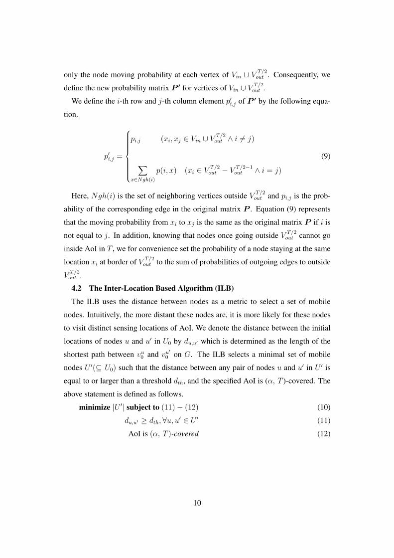
4.2 The Inter-Location Based Algorithm (ILB)

The ILB uses the distance between nodes as a metric to select a set of mobile

nodes. Intuitively, the more distant these nodes are, it is more likely for these nodes

to visit distinct sensing locations of AoI. We denote the distance between the initial

locations of nodes u and u′ in U0 by du,u′ which is determined as the length of the

shortest path between vu0 and vu′

0 on G. The ILB selects a minimal set of mobile

nodes U ′(⊆ U0) such that the distance between any pair of nodes u and u′ in U ′ is

equal to or larger than a threshold dth, and the specified AoI is (α, T )-covered. The

above statement is defined as follows.

minimize |U ′| subject to (11)− (12) (10)

du,u′ ≥ dth, ∀u, u′ ∈ U ′ (11)

AoI is (α, T )-covered (12)

10

Algorithm 1 The Inter-location based algorithm (ILB)Input: U , AoI , α, T , G = (V,E)

Output: U ′

1: U ′ ← ∅2: Compose Vin, V T/2

out , U0 from AoI and U

3: P ← ComputeProbMatrix(AoI ,Vin ∪ VT/2out )

4: for ∀u ∈ U0 do

5: Compose u’s initial state vector vu0

6: end for

7: dmax ← maxu,u′∈U0

{du,u′}8: dth ← min( T

α·dmax, dmax)

9: while SetProb(v, U ′, T ) < α,∀v ∈ Vin do

10: if U0 = ∅ then

11: return ∅12: end if

13: Select u ∈ U0 at random

14: if U ′ = ∅ or minu′∈U ′{du,u′} ≥ dth then

15: U ′ ← U ′ ∪ {u}, U0 ← U0 − {u}16: end if

17: end while

18: return U ′

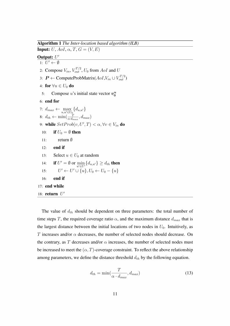
The value of dth should be dependent on three parameters: the total number of

time steps T , the required coverage ratio α, and the maximum distance dmax that is

the largest distance between the initial locations of two nodes in U0. Intuitively, as

T increases and/or α decreases, the number of selected nodes should decrease. On

the contrary, as T decreases and/or α increases, the number of selected nodes must

be increased to meet the (α, T )-coverage constraint. To reflect the above relationship

among parameters, we define the distance threshold dth by the following equation.

dth = min(T

α · dmax

, dmax) (13)

11

Algorithm 1 shows the node selection process of ILB. The input parameters are

the set of mobile nodes U , the area of interest AoI , the required coverage ratio α, the

query interval time T , and the service area graph G = (V,E). In line 1, the algorithm

initializes U ′ to be empty. In line 2, it composes the sets of vertices Vin and VT/2out , and

the set of nodes in the AoI, U0. In line 3, it composes the probability matrix P . In

lines 4 to 6, it composes the initial state vector for each node u ∈ U0. In lines 7 and

8, the algorithm determines the maximum distance dmax between nodes in U0 and

the distance threshold dth, as defined in equation (13). In lines 9 to 18, the algorithm

selects a set of nodes U ′ as follows: (i) while the AoI is not (α, T )-covered, the

algorithm checks the state of U0 and if U0 is empty, the algorithm returns ∅ (i.e., the

current U0 is not sufficient to satisfy the required coverage α), as shown in lines 9

to 12, (ii) the algorithm selects a node u ∈ U0 at random, as shown in line 13; and

(iii) it adds the node u to the selected set of nodes U ′ if U ′ is empty or the distance

between u and each node u′ ∈ U ′ is no less than the threshold dth, as shown in lines

14 to 16. Finally, in line 18, the algorithm returns the selected set of nodes U ′.

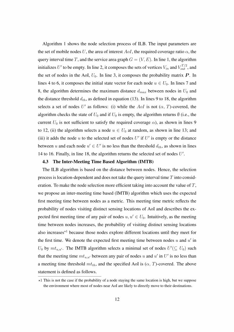
4.3 The Inter-Meeting Time Based Algorithm (IMTB)

The ILB algorithm is based on the distance between nodes. Hence, the selection

process is location-dependent and does not take the query interval time T into consid-

eration. To make the node selection more efficient taking into account the value of T ,

we propose an inter-meeting time based (IMTB) algorithm which uses the expected

first meeting time between nodes as a metric. This meeting time metric reflects the

probability of nodes visiting distinct sensing locations of AoI and describes the ex-

pected first meeting time of any pair of nodes u, u′ ∈ U0. Intuitively, as the meeting

time between nodes increases, the probability of visiting distinct sensing locations

also increases⋆1 because those nodes explore different locations until they meet for

the first time. We denote the expected first meeting time between nodes u and u′ in

U0 by mtu,u′ . The IMTB algorithm selects a minimal set of nodes U ′(⊆ U0) such

that the meeting time mtu,u′ between any pair of nodes u and u′ in U ′ is no less than

a meeting time threshold mtth, and the specified AoI is (α, T )-covered. The above

statement is defined as follows.

⋆1 This is not the case if the probability of a node staying the same location is high, but we supposethe environment where most of nodes near AoI are likely to directly move to their destinations.

12

minimize |U ′| subject to (15)− (16) (14)

mtu,u′ ≥ mtth, ∀u, u′ ∈ U ′ (15)

AoI is (α, T )-covered (16)

Algorithm 2 The Iner-meeting time based algorithm (IMTB)Input: U , AoI , α, T , G = (V,E)

Output: U ′

1: U ′ ← ∅2: Compose Vin, V T/2

out , U0 from AoI and U

3: P ← ComputeProbMatrix(AoI ,Vin ∪ VT/2out )

4: for ∀u ∈ U0 do

5: compose u’s initial state vector vu0

6: end for

7: mtmax ← maxu,u′∈U0{mtu,u′ : mtu,u′ ̸=∞}8: mtth ← min( T

α·mtmax,mtmax)

9: while SetProb(v, U ′, T ) < α,∀v ∈ Vin do

10: if U0 = ∅ then

11: return ∅12: end if

13: Select u ∈ U0 at random

14: if U ′ = ∅ or minu′∈U ′{mtu,u′} ≥ mtth then

15: U ′ ← U ′ ∪ {u}, U0 ← U0 − {u}16: end if

17: end while

18: return U ′

The values of mtu,u′ and mtth are calculated as follows.

The expected first meeting time mtu,u′ represents the earliest time when two nodes

u and u′ in U0 may meet at some location vt ∈ Vin and is defined by the following

equation.

13

mtu,u′ =

min

t∈MTu,u′{t} (MTu,u′ ̸= ∅)

T (MTu,u′ = ∅)(17)

where MTu,u′ is a set of possible meeting time between u and u′ during the time

period T and is defined by the following equation.

MTu,u′ = {t | Prob(u, t, vu0 , vt) > 0 ∧ Prob(u′, t, vu′

0 , vt) > 0, 0 ≤ t ≤ T,(18)

∃ vt ∈ AoI}

The meeting time threshold mtth should be dependent on three parameters: the

total number of time steps T , the required coverage ratio α, and the maximum ex-

pected first meeting time mtmax between pairs of nodes in U0. Intuitively, as T

increases and/or α decreases, the number of selected nodes will decrease. To reflect

the above relationship among parameters, we define the meeting time threshold mtth

as follows.

mtth = min(T

α ·mtmax

,mtmax) (19)

Algorithm 2 shows the node selection process of IMTB. The input parameters are

the same as in Algorithm 1. In lines 1 to 6, the algorithm does the same steps as

lines 1 to 6 in Algorithm 1. In lines 7 and 8, the algorithm determines the maximum

expected first meeting time mtmax between nodes in U0 and the threshold mtth, as

defined in equation (19). In lines 9 to 18, the algorithm selects a set of nodes U ′ as in

Algorithm 1, except in line 14, where it adds the node u to the selected set of nodes

U ′ if U ′ is empty or the expected first meeting time between u and each node u′ ∈ U ′

is no less than the threshold mtth.

4.4 The Extended Algorithm without Thresholds (EWOT)

As we described in the previous two subsections, ILB and IMTB algorithms apply

the selection process only on a set of nodes located inside AoI at time 0, U0, and

do not consider the nodes outside AoI. The number of nodes inside AoI at time 0

may not be sufficient to guarantee the α-coverage of AoI in time period T , if it is too

small.

14

Algorithm 3 The Extended Algorithm without Thresholds (EWOT)Input: U , AoI , α, T , G = (V,E)

Output: U ′

1: U ′ ← ∅2: Compose Vin, V T/2

out , U0, UT/20 from AoI and U

3: P ← ComputeProbMatrix(AoI ,Vin ∪ VT/2out )

4: for ∀u ∈ U0 ∪ UT/20 do

5: compose u’s initial state vector vu0

6: end for

7: while SetProb(v, U ′, T ) < α,∀v ∈ Vin do

8: if U0 ̸= ∅ then

9: Select u with the highest coverage contribution of U0

10: U ′ ← U ′ ∪ {u}, U0 ← U0 − {u}11: else if U0 = ∅ then

12: if UT/20 = ∅ then

13: return ∅14: end if

15: Select u with the highest coverage contribution of UT/20

16: U ′ ← U ′ ∪ {u}, UT/20 ← U

T/20 − {u}

17: end if

18: end while

19: return U ′

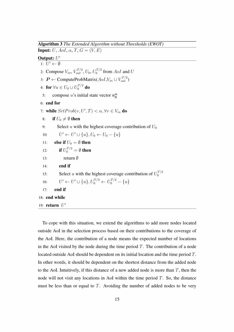
To cope with this situation, we extend the algorithms to add more nodes located

outside AoI in the selection process based on their contributions to the coverage of

the AoI. Here, the contribution of a node means the expected number of locations

in the AoI visited by the node during the time period T . The contribution of a node

located outside AoI should be dependent on its initial location and the time period T .

In other words, it should be dependent on the shortest distance from the added node

to the AoI. Intuitively, if this distance of a new added node is more than T , then the

node will not visit any locations in AoI within the time period T . So, the distance

must be less than or equal to T . Avoiding the number of added nodes to be very

15

large, we add only nodes if the shortest distance to the AoI is less than or equal to

⌊T2⌋. We denote the extended algorithm without thresholds by EWOT.

Algorithm 3 shows the node selection process of EWOT. The input parameters are

the same as in Algorithms 1 and 2. In line 1, the algorithm initializes U ′ to empty.

In line 2, it composes the sets of vertices Vin and VT/2out , and the sets of nodes U0 and

UT/20 (this contains all nodes that initially exist in V

T/2out ). In line 3, it composes the

probability matrix P . In lines 4 to 6, it composes the initial state vector for each node

u ∈ U0∪UT/20 . In lines 7 to 19, the algorithm selects a set of nodes U ′ as follows: (i)

while the AoI is not (α, T )-covered, if U0 is not empty, the algorithm selects a node

u with the highest coverage contribution of U0 and adds it to the selected set of nodes

U ′, as shown in lines 7 to 10. (ii) if U0 is empty (i.e., the current U0 is not sufficient

to satisfy the required coverage α), the algorithm checks the state of UT/20 , and if it is

empty, the algorithm returns ∅, as shown in lines 11 to 14, (iii) the algorithm selects

a node u with the highest coverage contribution of UT/20 , as shown in line 15; (iv) it

adds the node u to the selected set of nodes U ′, as shown in line 16. Finally, in line

19, the algorithm returns the selected set of nodes U ′.

4.5 The ILB and IMTB Algorithms with Updating Mechanism

As we described in the previous two subsections, the ILB and IMTB algorithms

are based only on the initial locations of nodes inside the AoI and do not consider

the latest locations of nodes during the query period T . There can be a scenario that

some nodes initially exist in the AoI and may go out of the AoI after some time

during the query period T . Also, some nodes may initially exist outside of the AoI

and may go into the AoI after some time during the query period T . If we track

the location of nodes in and near the AoI during period T , we can achieve more

accurate coverage with lower cost by removing useless nodes and adding some extra

nodes that more contribute coverage. For more accurate coverage, we propose an

updating mechanism for the ILB and IMTB algorithms that aims to adapt the number

of selected nodes based on the latest location of nodes. This updating mechanism is

executed every specified time interval during the time period T .

Let tcurrent denote the current time step. The updating mechanism consists of the

following steps

16

( 1 ) Calculate the remaining required coverage ratio, β⋆1 (β = α − γ, where γ is

the already achieved coverage ratio).

( 2 ) Estimate the coverage probability for all uncovered locations in AoI by the

nodes in U ′ if their current locations exist in AoI by using the ILB or IMTB

algorithms.

( 3 ) If the estimated coverage probability is less than β, then one-by-one add a

new node to the selected set while all locations in AoI are (β, T − tcurrent)-

covered.

( 4 ) If the estimated coverage probability is larger than β, then one-by-one remove

a node from U ′ as long as all uncovered locations in AoI are (β, T − tcurrent)-

covered.

By using this updating mechanism, the ILB and IMTB algorithms can adapt the

number of selected nodes by adding or removing some nodes to improve the accuracy

of the coverage probability of AoI as much as possible. This updating mechanism is

executed periodically every specified time interval which called the updating interval

UI .

The value of UI is preferable to be determined internally. In other words, it should

be dependent on T and α. So, we use the distance threshold dth and the meeting

time threshold mtth of ILB, and IMTB, respectively to determine the value of UI as

follows.

UI =

dth for ILB

mtth for IMTB(20)

We refer to the ILB and IMTB with the updating mechanism by ILB-up and IMTB-

up, respectively.

4.6 Complexity

Here, we evaluate the computing time of the proposed algorithms according to the

size of matrix P , (M + L)2 , the number of nodes in U0 (i.e., inside AoI), n, and

the total number of steps, T . According to coverage probability of a vertex which is

defined in Equation (7), the computing time of ILB and IMTB is O (n·(M+L)2 ·T ),while the computing time for EWOT is O((n+ n′) · (M + L)2 · T ), where n′ is the

⋆1 Here, to minimize the total overhead, β represents the maximum deficit coverage ratio among alllocations in AoI.

17

number of nodes in UT/20 (i.e., outside AoI).

5. Performance Evaluation

In this section, we show the results of simulation experiments that examine the

coverage performance of the proposed algorithms in terms of the number of nodes

selected and the accuracy of the achieved coverage ratio. We compared the proposed

algorithms with the random selection method which repeats selecting a node ran-

domly among all nodes inside AoI until satisfying (α, T )-coverage and does not use

any distance or time thresholds.

Table 2: Configuration Parameters.

Configuration parameter Value in simulation

# nodes 25 to 200

Node speed 1 m/s

Field size 500m× 500m

Required coverage, α 0.2, 0.4, 0.5, 0.6, 0.8, 0.9

Total # sensing locations in A 121

AoI-Size (# sensing locations) 0.01 (4), 0.25 (36), 0.45 (56),

0.5 (66), 0.65 (77), 0.85 (99)

∆ 50 m

Total # steps (time period), T 2, 4, 6,..., 20

5.1 Simulation Environment

The QualNet19) simulator was used with the input parameters listed in Table 2, such

as service area size, number of nodes, node speed, etc. In addition, the node mobility

was based on a discrete Markov model as described in Section 4. The service area

was represented as a grid of sensing locations arranged with uniform spacing, 50

meters. We selected the AoI as a rectangular region where its position was selected

at random within the service area. The ratio of its size to the service area size, called

AoI-Size, was selected from {0.01, 0.25, 0.45, 0.5, 0.65, 0.85} and the corresponding

number of sensing locations in each AoI was {4, 36, 56, 66, 77, 99}. The initial node

location was selected at random among all sensing locations in the service area. We

18

(a) Number of selected nodes (b) Achieved coverage ratio

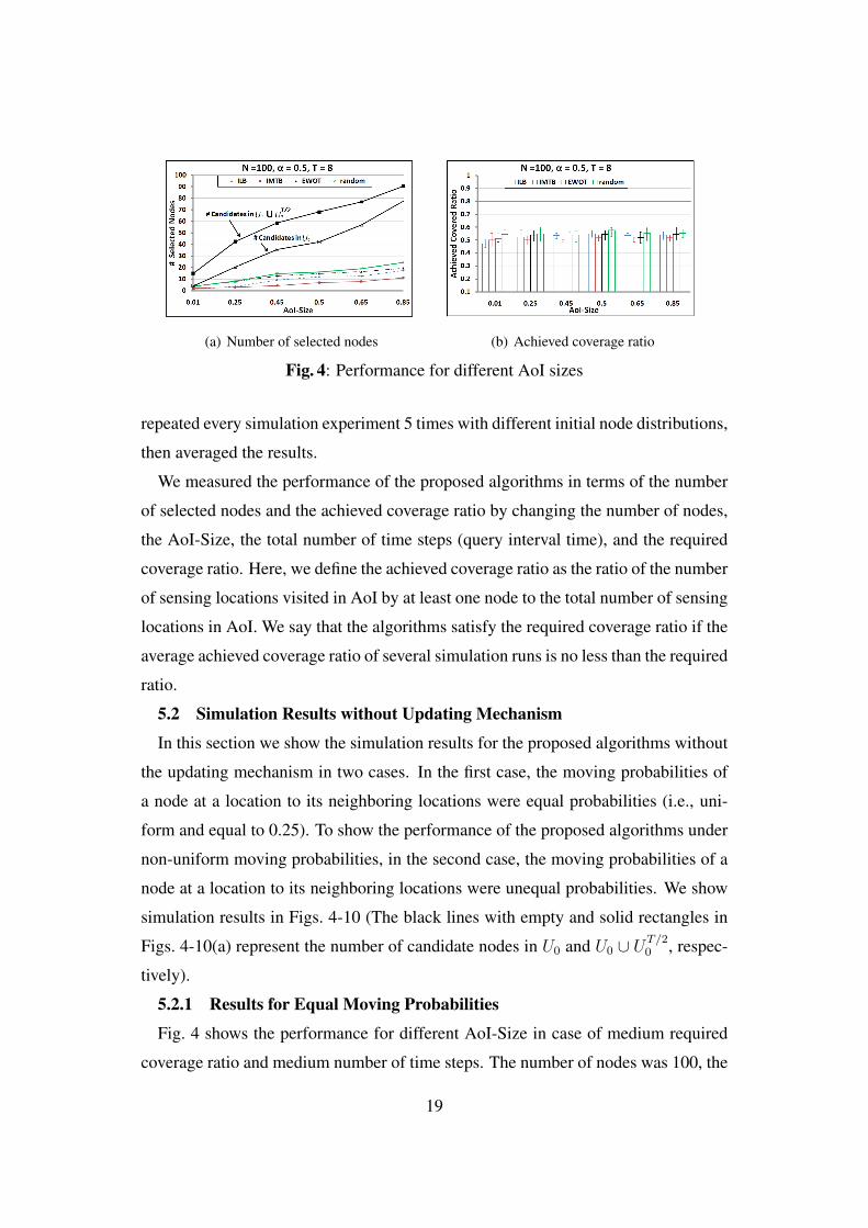
Fig. 4: Performance for different AoI sizes

repeated every simulation experiment 5 times with different initial node distributions,

then averaged the results.

We measured the performance of the proposed algorithms in terms of the number

of selected nodes and the achieved coverage ratio by changing the number of nodes,

the AoI-Size, the total number of time steps (query interval time), and the required

coverage ratio. Here, we define the achieved coverage ratio as the ratio of the number

of sensing locations visited in AoI by at least one node to the total number of sensing

locations in AoI. We say that the algorithms satisfy the required coverage ratio if the

average achieved coverage ratio of several simulation runs is no less than the required

ratio.

5.2 Simulation Results without Updating Mechanism

In this section we show the simulation results for the proposed algorithms without

the updating mechanism in two cases. In the first case, the moving probabilities of

a node at a location to its neighboring locations were equal probabilities (i.e., uni-

form and equal to 0.25). To show the performance of the proposed algorithms under

non-uniform moving probabilities, in the second case, the moving probabilities of a

node at a location to its neighboring locations were unequal probabilities. We show

simulation results in Figs. 4-10 (The black lines with empty and solid rectangles in

Figs. 4-10(a) represent the number of candidate nodes in U0 and U0 ∪ UT/20 , respec-

tively).

5.2.1 Results for Equal Moving Probabilities

Fig. 4 shows the performance for different AoI-Size in case of medium required

coverage ratio and medium number of time steps. The number of nodes was 100, the

19

(a) Number of selected nodes (b) Achieved coverage ratio

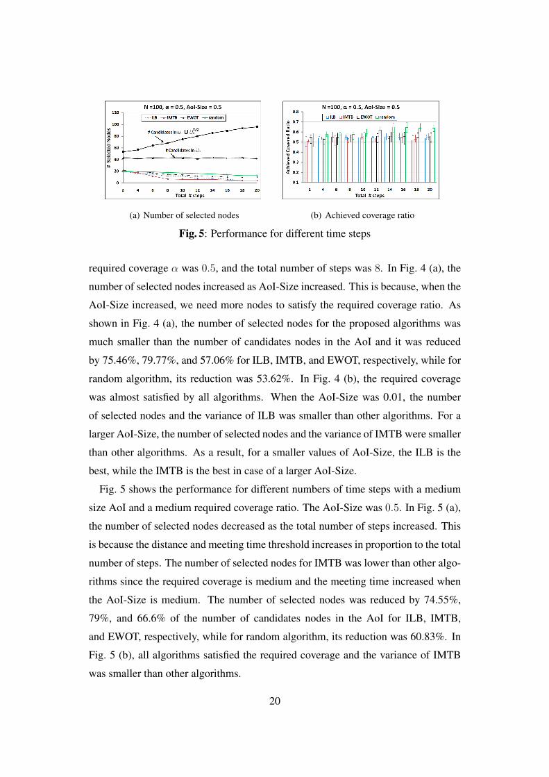
Fig. 5: Performance for different time steps

required coverage α was 0.5, and the total number of steps was 8. In Fig. 4 (a), the

number of selected nodes increased as AoI-Size increased. This is because, when the

AoI-Size increased, we need more nodes to satisfy the required coverage ratio. As

shown in Fig. 4 (a), the number of selected nodes for the proposed algorithms was

much smaller than the number of candidates nodes in the AoI and it was reduced

by 75.46%, 79.77%, and 57.06% for ILB, IMTB, and EWOT, respectively, while for

random algorithm, its reduction was 53.62%. In Fig. 4 (b), the required coverage

was almost satisfied by all algorithms. When the AoI-Size was 0.01, the number

of selected nodes and the variance of ILB was smaller than other algorithms. For a

larger AoI-Size, the number of selected nodes and the variance of IMTB were smaller

than other algorithms. As a result, for a smaller values of AoI-Size, the ILB is the

best, while the IMTB is the best in case of a larger AoI-Size.

Fig. 5 shows the performance for different numbers of time steps with a medium

size AoI and a medium required coverage ratio. The AoI-Size was 0.5. In Fig. 5 (a),

the number of selected nodes decreased as the total number of steps increased. This

is because the distance and meeting time threshold increases in proportion to the total

number of steps. The number of selected nodes for IMTB was lower than other algo-

rithms since the required coverage is medium and the meeting time increased when

the AoI-Size is medium. The number of selected nodes was reduced by 74.55%,

79%, and 66.6% of the number of candidates nodes in the AoI for ILB, IMTB,

and EWOT, respectively, while for random algorithm, its reduction was 60.83%. In

Fig. 5 (b), all algorithms satisfied the required coverage and the variance of IMTB

was smaller than other algorithms.

20

(a) Number of selected nodes (b) Achieved coverage ratio

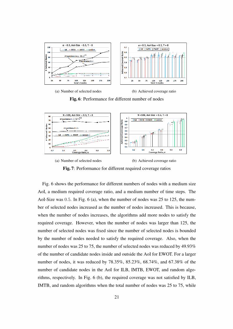
Fig. 6: Performance for different number of nodes

(a) Number of selected nodes (b) Achieved coverage ratio

Fig. 7: Performance for different required coverage ratios

Fig. 6 shows the performance for different numbers of nodes with a medium size

AoI, a medium required coverage ratio, and a medium number of time steps. The

AoI-Size was 0.5. In Fig. 6 (a), when the number of nodes was 25 to 125, the num-

ber of selected nodes increased as the number of nodes increased. This is because,

when the number of nodes increases, the algorithms add more nodes to satisfy the

required coverage. However, when the number of nodes was larger than 125, the

number of selected nodes was fixed since the number of selected nodes is bounded

by the number of nodes needed to satisfy the required coverage. Also, when the

number of nodes was 25 to 75, the number of selected nodes was reduced by 49.93%

of the number of candidate nodes inside and outside the AoI for EWOT. For a larger

number of nodes, it was reduced by 78.35%, 85.23%, 68.74%, and 67.38% of the

number of candidate nodes in the AoI for ILB, IMTB, EWOT, and random algo-

rithms, respectively. In Fig. 6 (b), the required coverage was not satisfied by ILB,

IMTB, and random algorithms when the total number of nodes was 25 to 75, while

21

the EWOT algorithm satisfied the required coverage with small variance. This is be-

cause EWOT algorithm takes into account nodes that also exist outside AoI and it

can add more nodes to meet the required coverage. For a larger number of nodes, all

algorithms satisfied the required coverage and the variance of IMTB was smaller than

other algorithms. As a result, for a small number of nodes inside AoI, the EWOT is

the best, while the IMTB is the best in case of a larger number of nodes.

Fig. 7 shows the performance for different required coverage ratio with medium

size AoI and medium number of time steps. The AoI-Size was 0.5. In Fig. 7 (a),

the number of selected nodes increased as required coverage ratio increased. This is

because, as the required coverage ratio increases, we need more nodes to satisfy it.

The number of selected nodes for IMTB was lower than other algorithms and it was

reduced by 76.68% of the number candidate nodes in the AoI. On the other hand, it

was reduced by 69.46%, 58%, and 50.45% for ILB, EWOT, and random algorithms,

respectively. In Fig. 7 (b), the required coverage was satisfied by all algorithms and

the variance of IMTB is smaller than other algorithms.

Here, we summarize the simulation results as follows.

• ILB, IMTB, and EWOT algorithms reduce the number of selected nodes to a

great extent for (α, T )-coverage compared to the number of candidate nodes in

the AoI.

• For a small AoI, ILB can select a smaller number of nodes to meet the required

coverage with smaller variance than IMTB, EWOT, and random algorithms.

• For medium and large AoI, IMTB can select smaller number of nodes to meet

the required coverage with smaller variance than ILB, EWOT, and random al-

gorithms..

• When only a small number of nodes are initially located in the AoI, only the

EWOT algorithm can meet the required coverage.

5.2.2 Results for Unequal Moving Probabilities

In the real environment, the moving probabilities of a node at any location to its

neighboring are almost unequal. In order to investigate to what extent the unequal-

ness of the moving probability affects the performance of the proposed methods, we

conducted simulations according to the following two scenarios.

• a) random moving probabilities: in this scenario, the moving probability of a

22

node at a location i to one of its neighboring locations is determined randomly

between 0.01 and 0.09 such that the sum of all moving probabilities to its neigh-

boring locations is equal to 1.

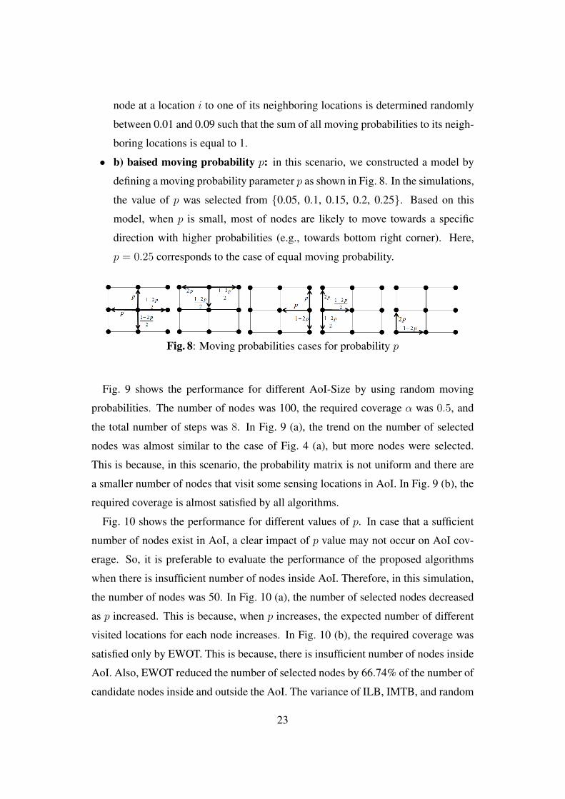
• b) baised moving probability p: in this scenario, we constructed a model by

defining a moving probability parameter p as shown in Fig. 8. In the simulations,

the value of p was selected from {0.05, 0.1, 0.15, 0.2, 0.25}. Based on this

model, when p is small, most of nodes are likely to move towards a specific

direction with higher probabilities (e.g., towards bottom right corner). Here,

p = 0.25 corresponds to the case of equal moving probability.

Fig. 8: Moving probabilities cases for probability p

Fig. 9 shows the performance for different AoI-Size by using random moving

probabilities. The number of nodes was 100, the required coverage α was 0.5, and

the total number of steps was 8. In Fig. 9 (a), the trend on the number of selected

nodes was almost similar to the case of Fig. 4 (a), but more nodes were selected.

This is because, in this scenario, the probability matrix is not uniform and there are

a smaller number of nodes that visit some sensing locations in AoI. In Fig. 9 (b), the

required coverage is almost satisfied by all algorithms.

Fig. 10 shows the performance for different values of p. In case that a sufficient

number of nodes exist in AoI, a clear impact of p value may not occur on AoI cov-

erage. So, it is preferable to evaluate the performance of the proposed algorithms

when there is insufficient number of nodes inside AoI. Therefore, in this simulation,

the number of nodes was 50. In Fig. 10 (a), the number of selected nodes decreased

as p increased. This is because, when p increases, the expected number of different

visited locations for each node increases. In Fig. 10 (b), the required coverage was

satisfied only by EWOT. This is because, there is insufficient number of nodes inside

AoI. Also, EWOT reduced the number of selected nodes by 66.74% of the number of

candidate nodes inside and outside the AoI. The variance of ILB, IMTB, and random

23

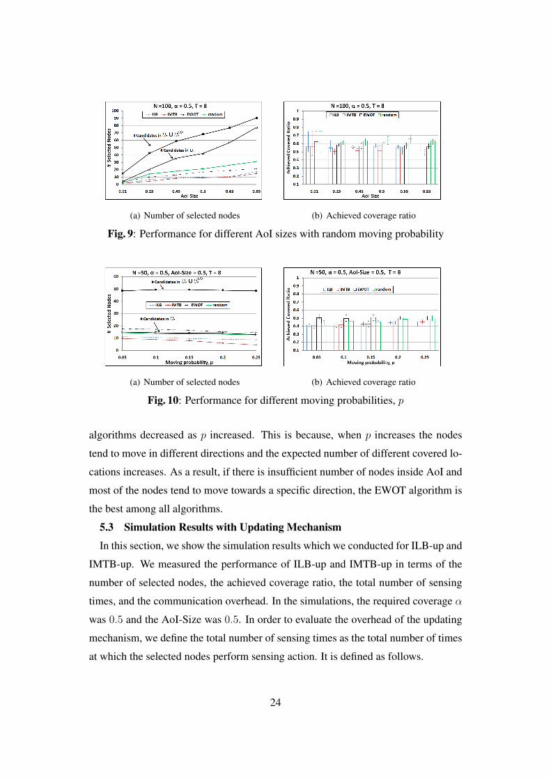
(a) Number of selected nodes (b) Achieved coverage ratio

Fig. 9: Performance for different AoI sizes with random moving probability

(a) Number of selected nodes (b) Achieved coverage ratio

Fig. 10: Performance for different moving probabilities, p

algorithms decreased as p increased. This is because, when p increases the nodes

tend to move in different directions and the expected number of different covered lo-

cations increases. As a result, if there is insufficient number of nodes inside AoI and

most of the nodes tend to move towards a specific direction, the EWOT algorithm is

the best among all algorithms.

5.3 Simulation Results with Updating Mechanism

In this section, we show the simulation results which we conducted for ILB-up and

IMTB-up. We measured the performance of ILB-up and IMTB-up in terms of the

number of selected nodes, the achieved coverage ratio, the total number of sensing

times, and the communication overhead. In the simulations, the required coverage α

was 0.5 and the AoI-Size was 0.5. In order to evaluate the overhead of the updating

mechanism, we define the total number of sensing times as the total number of times

at which the selected nodes perform sensing action. It is defined as follows.

24

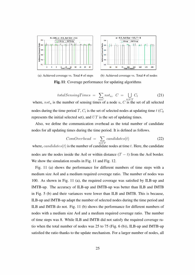
(a) Achieved coverage vs. Total # of steps (b) Achieved coverage vs. Total # of nodes

Fig. 11: Coverage performance for updating algorithms

totalSensingT imes =∑u∈C

nstu, C =∪

t∈UT

Ct (21)

where, nstu is the number of sensing times of a node u, C is the set of all selected

nodes during the time period T , Ct is the set of selected nodes at updating time t (C0

represents the initial selected set), and UT is the set of updating times.

Also, we define the communication overhead as the total number of candidate

nodes for all updating times during the time period. It is defined as follows.

ComOverhead =∑t∈UT

candidates(t) (22)

where, candidates(t) is the number of candidate nodes at time t. Here, the candidate

nodes are the nodes inside the AoI or within distance (T − t) from the AoI border.

We show the simulation results in Fig. 11 and Fig. 12.

Fig. 11 (a) shows the performance for different numbers of time steps with a

medium size AoI and a medium required coverage ratio. The number of nodes was

100. As shown in Fig. 11 (a), the required coverage was satisfied by ILB-up and

IMTB-up. The accuracy of ILB-up and IMTB-up was better than ILB and IMTB

in Fig. 5 (b) and their variances were lower than ILB and IMTB. This is because,

ILB-up and IMTB-up adapt the number of selected nodes during the time period and

ILB and IMTB do not. Fig. 11 (b) shows the performance for different numbers of

nodes with a medium size AoI and a medium required coverage ratio. The number

of time steps was 8. While ILB and IMTB did not satisfy the required coverage ra-

tio when the total number of nodes was 25 to 75 (Fig. 6 (b)), ILB-up and IMTB-up

satisfied the ratio thanks to the update mechanism. For a larger number of nodes, all

25

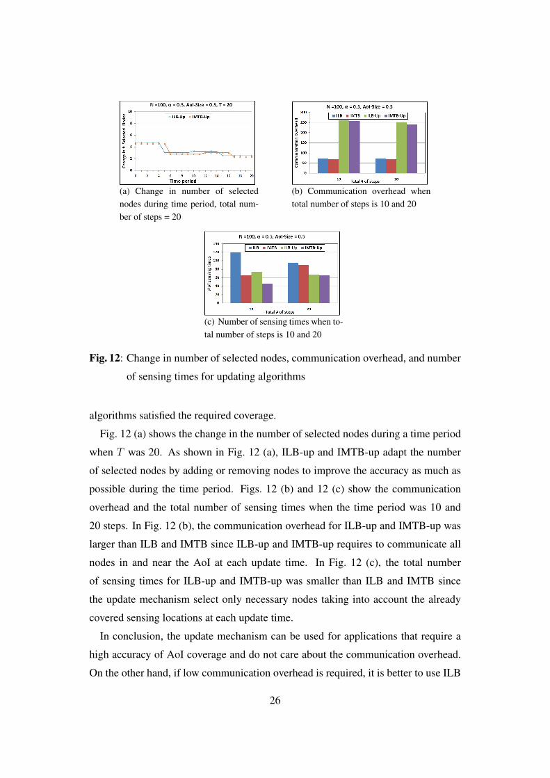
(a) Change in number of selectednodes during time period, total num-ber of steps = 20

(b) Communication overhead whentotal number of steps is 10 and 20

(c) Number of sensing times when to-tal number of steps is 10 and 20

Fig. 12: Change in number of selected nodes, communication overhead, and number

of sensing times for updating algorithms

algorithms satisfied the required coverage.

Fig. 12 (a) shows the change in the number of selected nodes during a time period

when T was 20. As shown in Fig. 12 (a), ILB-up and IMTB-up adapt the number

of selected nodes by adding or removing nodes to improve the accuracy as much as

possible during the time period. Figs. 12 (b) and 12 (c) show the communication

overhead and the total number of sensing times when the time period was 10 and

20 steps. In Fig. 12 (b), the communication overhead for ILB-up and IMTB-up was

larger than ILB and IMTB since ILB-up and IMTB-up requires to communicate all

nodes in and near the AoI at each update time. In Fig. 12 (c), the total number

of sensing times for ILB-up and IMTB-up was smaller than ILB and IMTB since

the update mechanism select only necessary nodes taking into account the already

covered sensing locations at each update time.

In conclusion, the update mechanism can be used for applications that require a

high accuracy of AoI coverage and do not care about the communication overhead.

On the other hand, if low communication overhead is required, it is better to use ILB

26

and IMTB without the update mechanism.

6. Conclusion

In this paper, we tackled the (α, T )-coverage problem in people centric sensing

with a motivating application scenario. We formulated this problem as an optimiza-

tion problem with the objective of minimizing the number of selected nodes to meet

the demanded coverage ratio α within a query interval time T . To resolve this prob-

lem, we proposed heuristic algorithms.

Our simulation results showed that the proposed algorithms achieved (α, T )-coverage

with good accuracy for a variety of values of α, T , AoI size, and moving probability,

and that the inter-meeting time based algorithm selects a smaller number of nodes

without deteriorating coverage accuracy. Also, the proposed algorithms reduce the

cost (number of sensing times) to a great extent compared to the case of selecting all

nodes in the AoI. In addition, our updating mechanism adapts the number of selected

nodes by removing useless nodes and adding some extra nodes that contribute more

to AoI coverage.

In this paper, we considered only the case where a single query is issued at a

time. In future work, we will try to make the proposed algorithms adaptive in case

of multiple simultaneous queries to minimize the overhead.

References

1) Campbell, A., Eisenman, S., Lane, N., Miluzzo, E., Peterson, R., Lu, H.,

Zheng, X., Musolesi, M., Fodor, K. and Ahn, G.: The Rise of People-Centric

Sensing, IEEE Internet Computing Special Issue on Mesh Networks, Vol. 12,

No.4, pp.12–21 (2008).

2) Al-Karaki, J. N. and Kamal, A. E.: Routing Techniques in Wireless Sensor

Networks: A survey, IEEE Wireless Communications, Vol.11, No.6, pp.6–28

(2004).

3) Akkaya, K. and Younis, M.: A survey on Routing Protocols for Wireless Sensor

Networks, IEEE Wireless Communications, Vol.3, No.3, pp.325–349 (2005).

4) Lima, L. and Barros, J.: Random Walks on Sensor Networks, Proc. of the 5th

Intl. Syposium on Modeling and Optimization in Mobile, Ad hoc, and Wireless

27

Networks, pp.1–5 (2007).

5) Shah, R., Roy, S., Jain, S. and Brunette, W.: Data mules: Modeling a three-

tier architecture for sparse sensor networks, Proc. of IEEE Workshop on Sensor

Network Protocols and Applications, pp.30–41 (2003).

6) Katsuma, R., Murata, Y., Shibata, N., Yasumoto, K. and Ito, M.: Extending k-

Coverage Lifetime of Wireless Sensor Networks Using Mobile Sensor Nodes,

Proc. of the 5th IEEE Intl. Conf. on Wireless and Mobile Computing, Networking

and Communications (WiMob’09), pp.48–54 (2009).

7) Wang, W., Sirinivasan, V. and Chua, K.: Trade-offs Between Mobility and Den-

sity for Coverage in Wireless Sensor Networks, Proc. of the 5th IEEE Intl. Conf.

on Mobile Computing and Networking (MobiCom’07), pp.39–50 (2007).

8) Hull, B., Bychkovsky, V., Zhang, Y., Chen, K., Goraczko, M., Miu, A., Shih, E.,

Balakrishnan, H. and Madden, S.: CarTel: A Distributed Mobile Sensor Com-

puting System, Proc. of the 4th Intl. Conf. on Embedded Networked Sensor Sys-

tems, pp.125–138 (2006).

9) Murty, R., Gosain, A., Tierney, M., Brody, A., Fahad, A., Bers, J. and Welsh,

M.: CitySense: A Vision for an Urban-Scale Wireless Networking Testbed,

Proc. Intl. Conf. on Technologies for Homeland Security, pp.583–588 (2008).

10) Tuulos, V., Scheible, J. and Nyholm, H.: Combining Web, Mobile Phones and

Public Displays in Large-Scale: Manhattan Story Mashup, Proc. of the 5th Intl.

Conf. on Pervasive Computing, pp.37–54 (2007).

11) Lua, H., Lane, N., Eisenmanb, S. and Campbella, A.: Bubble-sensing: Binding

Sensing Tasks to The Physical World, Pervasive and Mobile Computing, Vol.6,

No.1, pp.58–71 (2010).

12) Shi, J., Zhang, R., Liu, Y. and Zhang, Y.: PriSense: privacy-preserving data

aggregation in people-centric urban sensing systems, Proc. of INFOCOM’10,

pp.758–766 (2010).

13) Cornelius, C., Kapadia, A., Kotz, D., Peebles, D., Shin, M. and Triandopoulos,

N.: Anonysense: privacy-aware people-centric sensing, Proc. of MobiSys08, pp.

211–224 (2008).

14) Abdelzaher, T.: Mobiscopes for human spaces, IEEE Pervasive Computing,

Vol.6, No.2, pp.20–29 (2007).

28

15) Ganti, R. K., Pham, N., Ahmadi, H., Nangia, S. and Abdelzaher, T. F.:

GreenGPS: a participatory sensing fuel-efficient maps application, Proc. of Mo-

biSys10, pp.151–164 (2010).

16) Ahmed, A., Yasumoto, K., Yamauchi, Y. and Ito, M.: Probabilistic Methods for

Spatio-Temporal Coverage in People-Centric Sensing, Proc. of the 55th Mobile

Computing and Ubiquities communications Workshop (MBL55), pp.1–8 (2010).

17) Gadelrab, A., Yasumoto, K., Yamauchi, Y. and Ito, M.: Distance and Time

Based Node Selection for Probabilistic Coverage in People-Centric Sensing,

Subbmited to the 8th Annual IEEE Communications Society Conference on Sen-

sor, Mesh and Ad Hoc Communications and Networks (SECON’11) (2011).

http://www.aist-nara.ac.jp/~yasumoto/tmp/secon2011-

submitted.pdf.

18) Vercellis, C.: A Probabilistic Analysis of The Set Covering Problem, Annals of

Operations Research, Vol.1, No.3, pp.255–271 (1984).

19) Scalable Network Technologies Inc.: Qualnet 4.0 network simulator (2007).

29