
Interactions of ions with mattermetronu.ulb.ac.be/npauly/Pauly/metronu/3 Part 1_2.pdf · ·...
75
Chapter II: Interactions of ions with matter 1
Transcript of Interactions of ions with mattermetronu.ulb.ac.be/npauly/Pauly/metronu/3 Part 1_2.pdf · ·...

Chapter II: Interactions of ions with matter
1
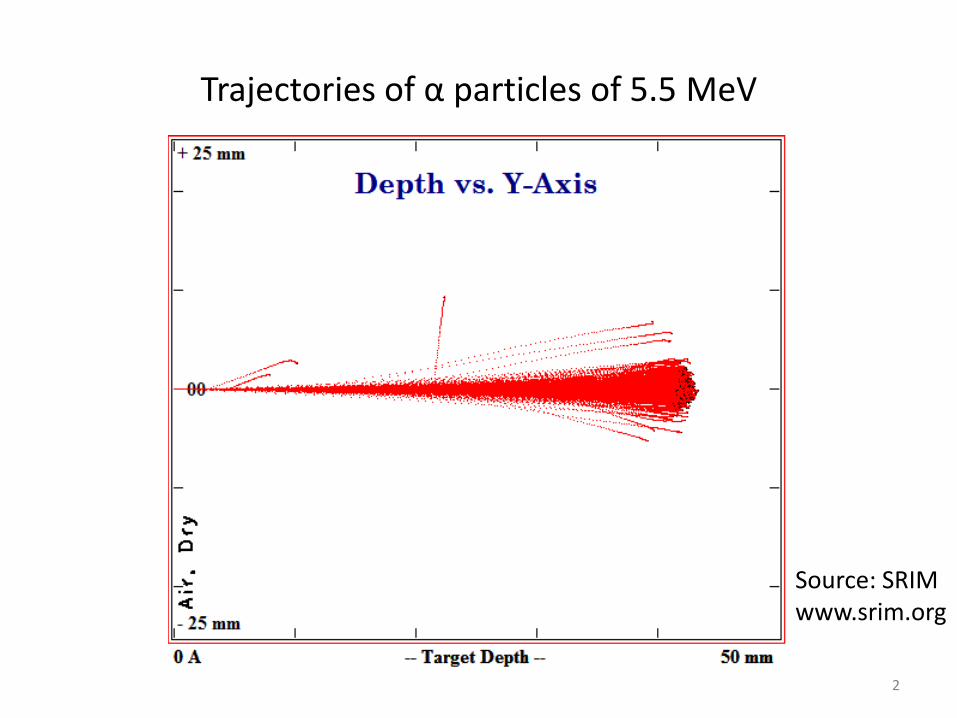
Trajectories of α particles of 5.5 MeV
2
Source: SRIM www.srim.org
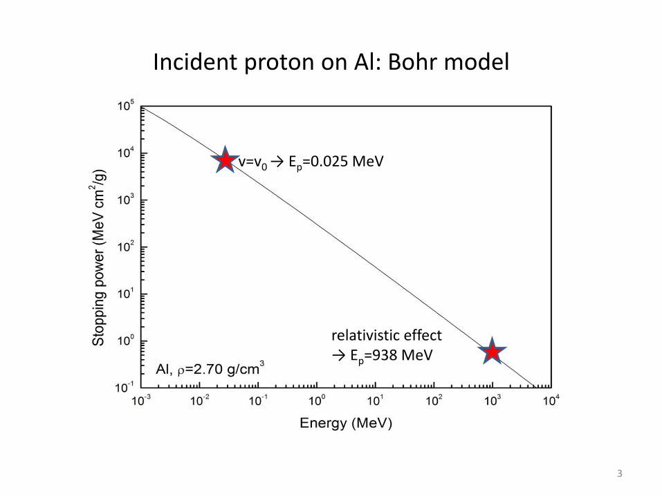
v=v0 → Ep=0.025 MeV
relativistic effect → Ep=938 MeV
Incident proton on Al: Bohr model
3
Contents
• Quantum model of the electronic stopping force
- Intermediate velocities
- Large velocities
- Small velocities
• Nuclear stopping force (small velocities)
• Range and Bragg curve
4
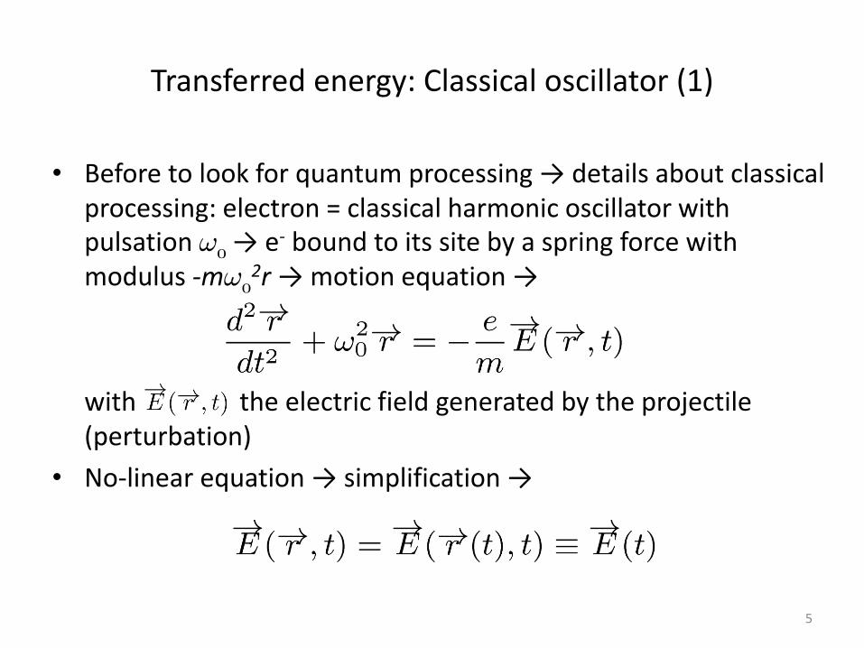
Transferred energy: Classical oscillator (1)
• Before to look for quantum processing → details about classical processing: electron = classical harmonic oscillator with pulsation !0 → e- bound to its site by a spring force with modulus -m!0
2r → motion equation →
with the electric field generated by the projectile (perturbation)
• No-linear equation → simplification →
5
Transferred energy: Classical oscillator (2)
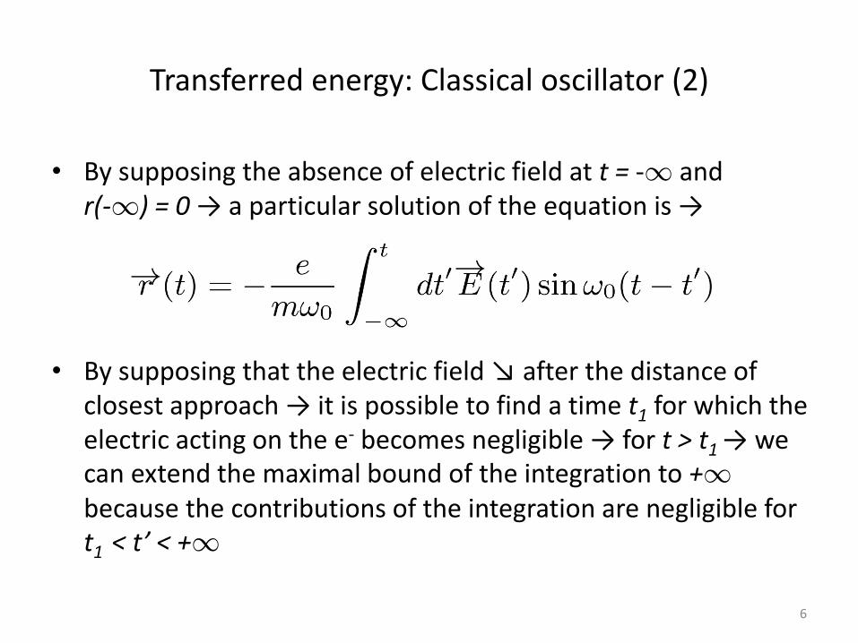
• By supposing the absence of electric field at t = -1 and r(-1) = 0 → a particular solution of the equation is →
• By supposing that the electric field ↘ after the distance of closest approach → it is possible to find a time t1 for which the electric acting on the e- becomes negligible → for t > t1 → we can extend the maximal bound of the integration to +1 because the contributions of the integration are negligible for t1 < t’ < +1
6
Transferred energy: Classical oscillator (3)
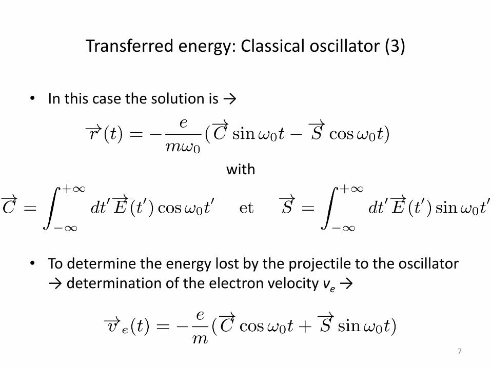
• In this case the solution is →
with
• To determine the energy lost by the projectile to the oscillator → determination of the electron velocity ve →
7
Transferred energy: Classical oscillator (4)
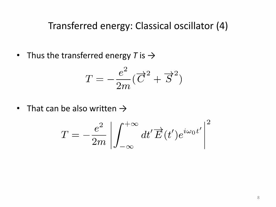
• Thus the transferred energy T is →
• That can be also written →
8
Classical oscillator: Dipolar approximation (1)
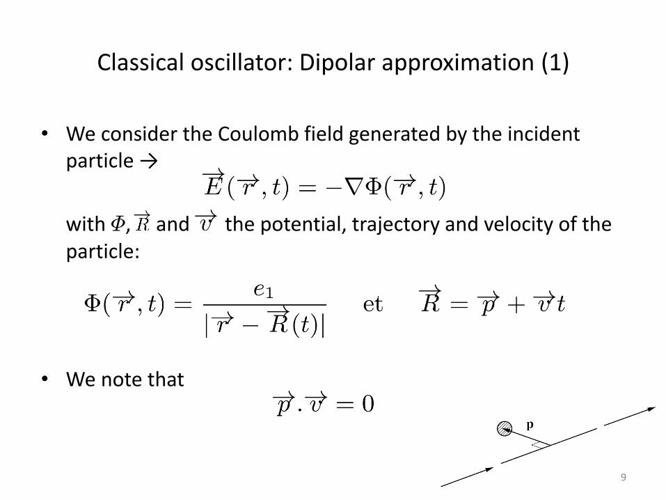
• We consider the Coulomb field generated by the incident particle →
with ©, and the potential, trajectory and velocity of the particle:
• We note that
9
Classical oscillator: Dipolar approximation (2)
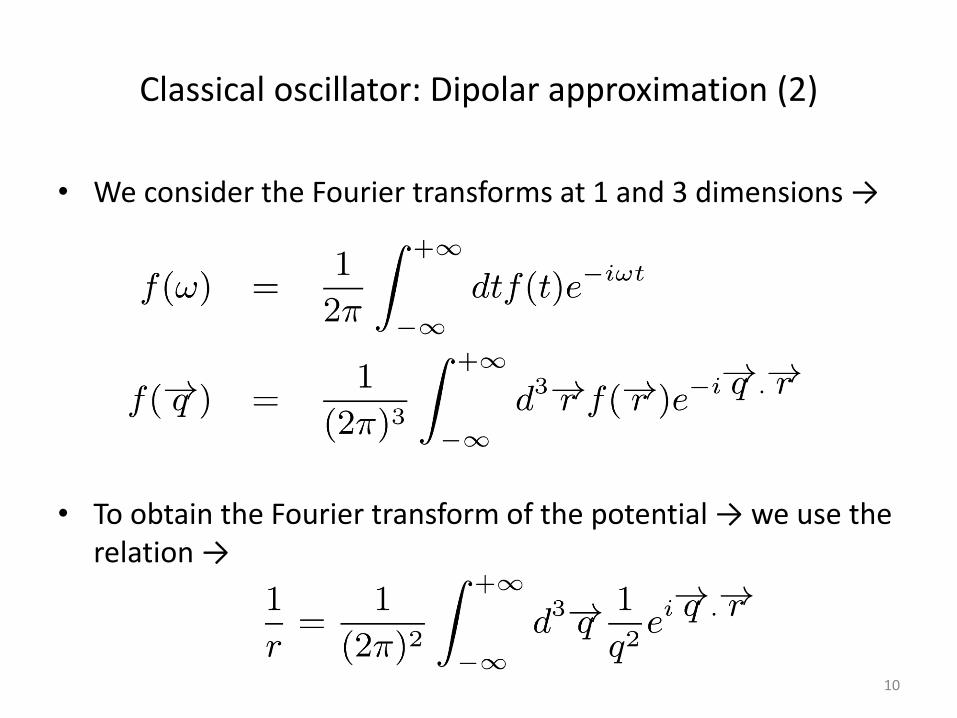
• We consider the Fourier transforms at 1 and 3 dimensions →
• To obtain the Fourier transform of the potential → we use the relation →
10
Classical oscillator: Dipolar approximation (3)
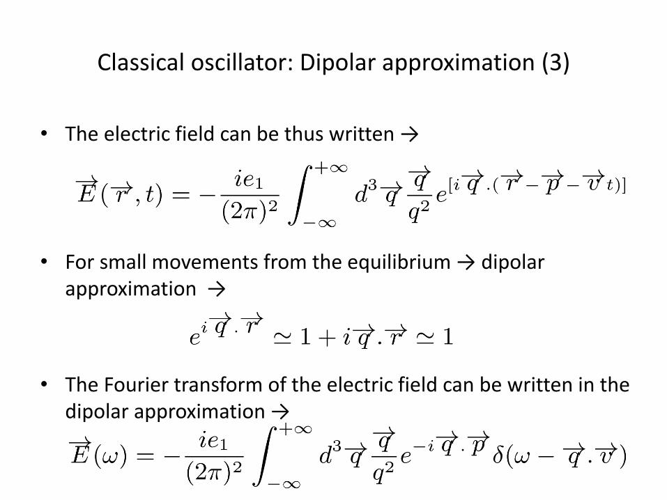
• The electric field can be thus written →
• For small movements from the equilibrium → dipolar approximation →
• The Fourier transform of the electric field can be written in the dipolar approximation →
11
Classical oscillator: Dipolar approximation (4)
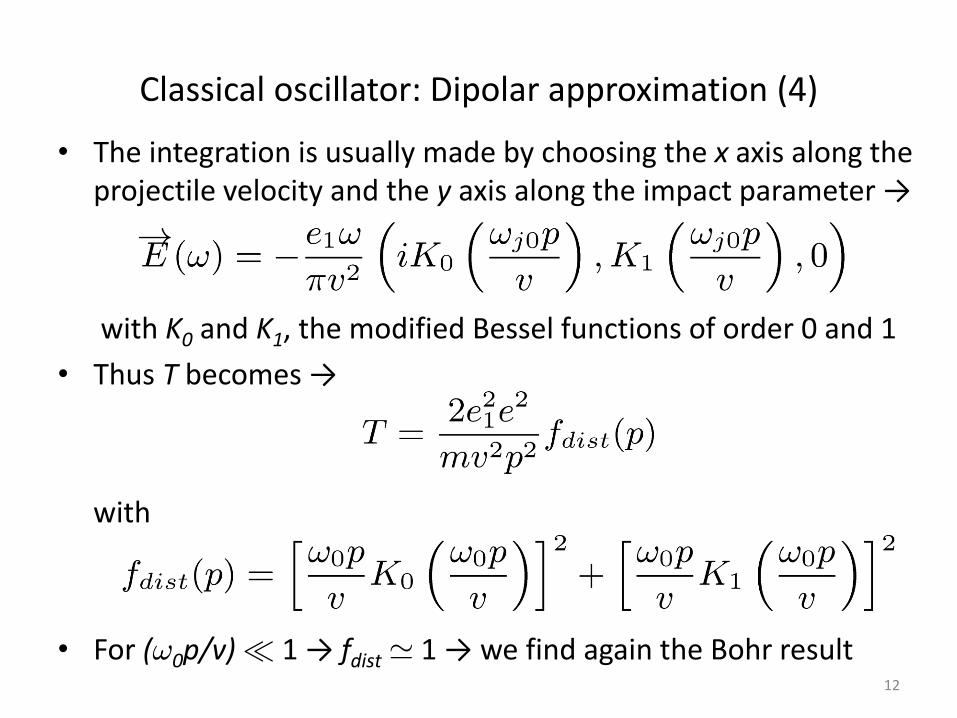
• The integration is usually made by choosing the x axis along the projectile velocity and the y axis along the impact parameter →
with K0 and K1, the modified Bessel functions of order 0 and 1
• Thus T becomes →
with
• For (!0p/v) ¿ 1 → fdist ' 1 → we find again the Bohr result 12
Semi-classical model for the stopping power: v0 ¿ v ¿ c (1)
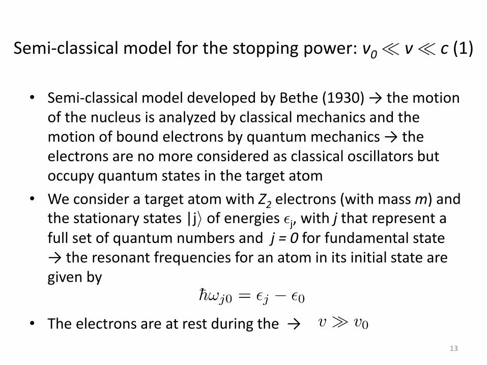
• Semi-classical model developed by Bethe (1930) → the motion of the nucleus is analyzed by classical mechanics and the motion of bound electrons by quantum mechanics → the electrons are no more considered as classical oscillators but occupy quantum states in the target atom
• We consider a target atom with Z2 electrons (with mass m) and the stationary states |ji of energies ²j, with j that represent a full set of quantum numbers and j = 0 for fundamental state → the resonant frequencies for an atom in its initial state are given by
• The electrons are at rest during the →
13
Semi-classical model for the stopping power: v0 ¿ v ¿ c (2)
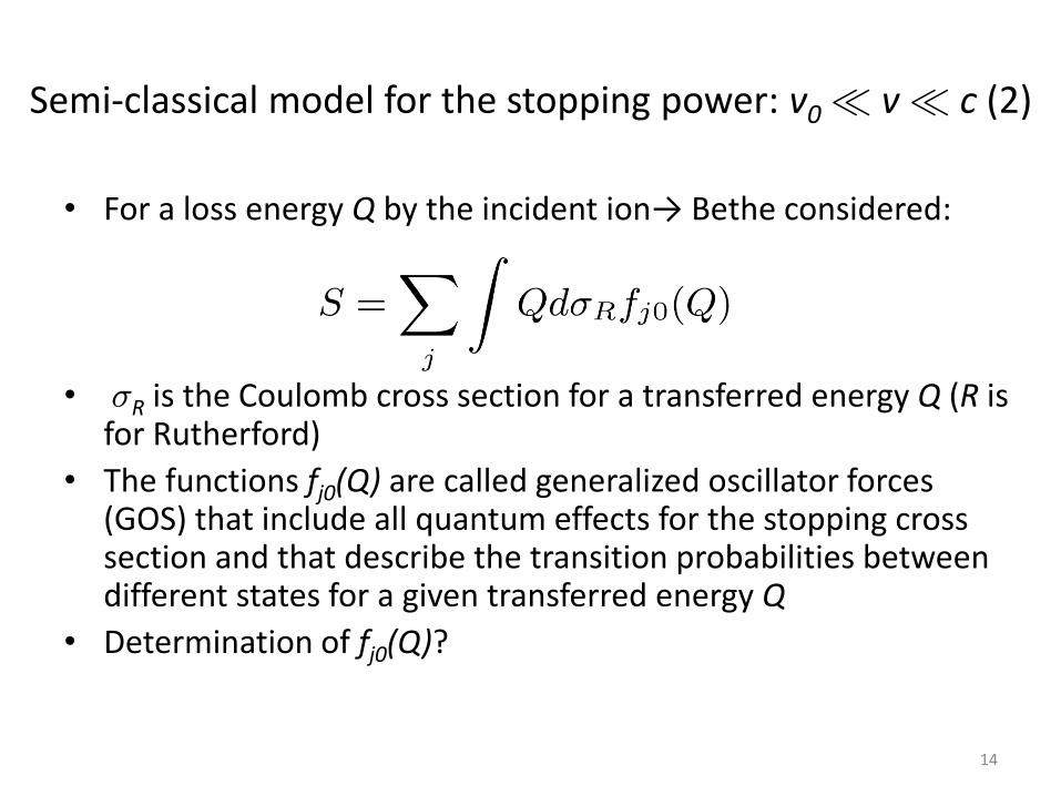
• For a loss energy Q by the incident ion→ Bethe considered:
• ¾R is the Coulomb cross section for a transferred energy Q (R is for Rutherford)
• The functions fj0(Q) are called generalized oscillator forces (GOS) that include all quantum effects for the stopping cross section and that describe the transition probabilities between different states for a given transferred energy Q
• Determination of fj0(Q)?
14
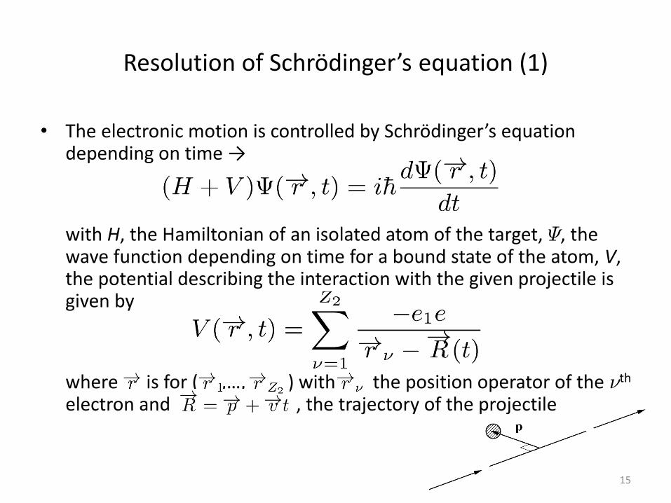
• The electronic motion is controlled by Schrödinger’s equation depending on time →
with H, the Hamiltonian of an isolated atom of the target, ª, the wave function depending on time for a bound state of the atom, V, the potential describing the interaction with the given projectile is given by
where is for ( ,…, ) with the position operator of the ºth electron and , the trajectory of the projectile
Resolution of Schrödinger’s equation (1)
15
Resolution of Schrödinger’s equation (2)
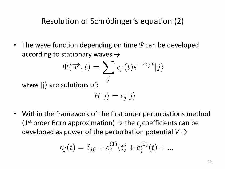
• The wave function depending on time ª can be developed according to stationary waves →
where |ji are solutions of:
• Within the framework of the first order perturbations method (1st order Born approximation) → the cj coefficients can be developed as power of the perturbation potential V →
16
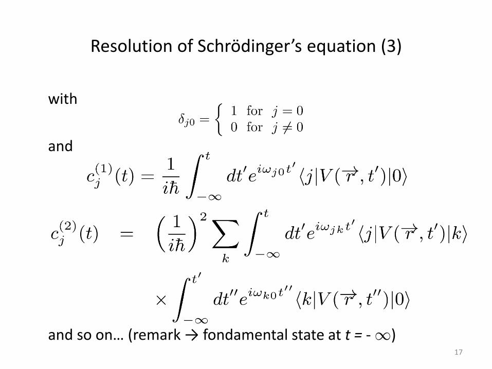
with
and
and so on… (remark → fondamental state at t = - 1)
Resolution of Schrödinger’s equation (3)
17
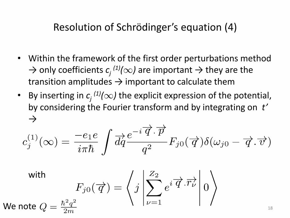
Resolution of Schrödinger’s equation (4)
• Within the framework of the first order perturbations method → only coefficients cj
(1)(1) are important → they are the transition amplitudes → important to calculate them
• By inserting in cj (1)(1) the explicit expression of the potential,
by considering the Fourier transform and by integrating on t’ →
with
18 We note
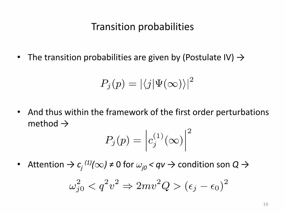
Transition probabilities
• The transition probabilities are given by (Postulate IV) →
• And thus within the framework of the first order perturbations method →
• Attention → cj (1)(1) ≠ 0 for !j0 < qv → condition son Q →
19
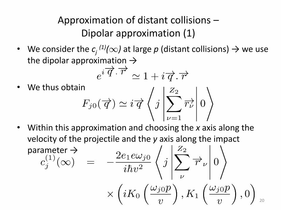
Approximation of distant collisions –Dipolar approximation (1)
• We consider the cj (1)(1) at large p (distant collisions) → we use
the dipolar approximation →
• We thus obtain
• Within this approximation and choosing the x axis along the velocity of the projectile and the y axis along the impact parameter →
20
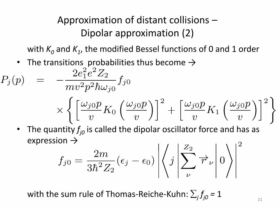
Approximation of distant collisions – Dipolar approximation (2)
with K0 and K1, the modified Bessel functions of 0 and 1 order
• The transitions probabilities thus become →
• The quantity fj0 is called the dipolar oscillator force and has as expression →
with the sum rule of Thomas-Reiche-Kuhn: j fj0 = 1 21
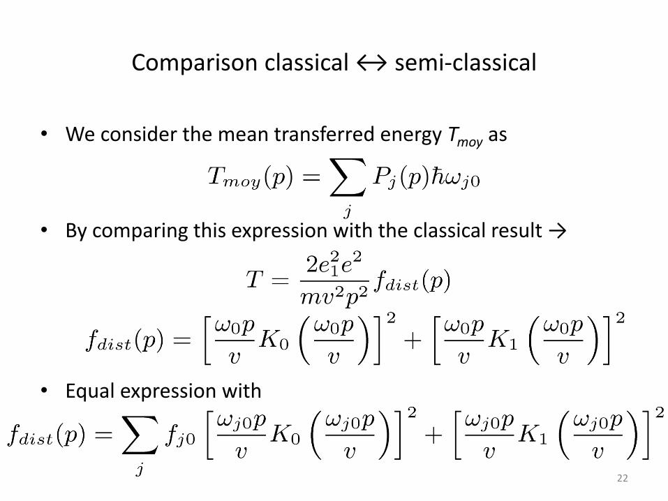
Comparison classical ↔ semi-classical
• We consider the mean transferred energy Tmoy as
• By comparing this expression with the classical result →
• Equal expression with
22
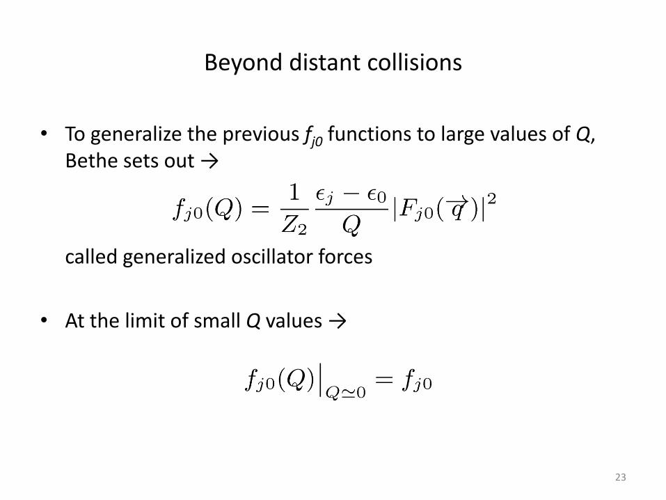
Beyond distant collisions
• To generalize the previous fj0 functions to large values of Q, Bethe sets out →
called generalized oscillator forces
• At the limit of small Q values →
23
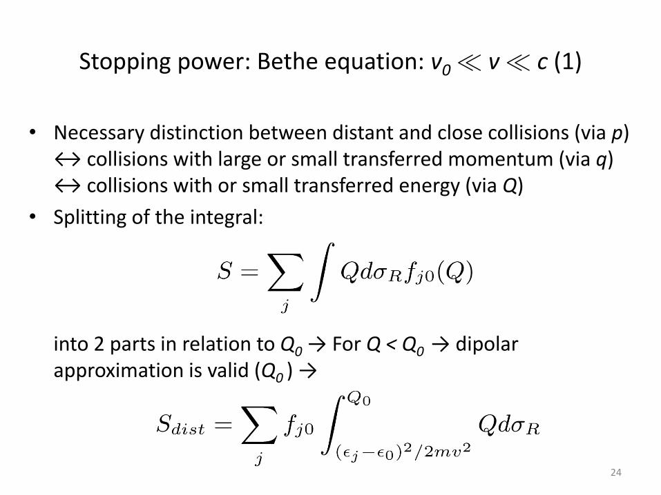
Stopping power: Bethe equation: v0 ¿ v ¿ c (1)
• Necessary distinction between distant and close collisions (via p) ↔ collisions with large or small transferred momentum (via q) ↔ collisions with or small transferred energy (via Q)
• Splitting of the integral:
into 2 parts in relation to Q0 → For Q < Q0 → dipolar approximation is valid (Q0 ) →
24
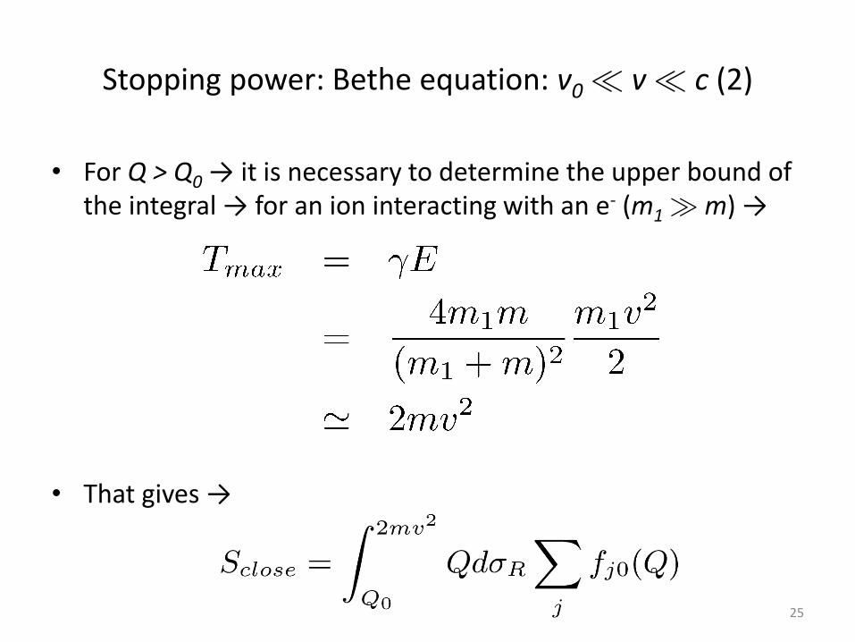
Stopping power: Bethe equation: v0 ¿ v ¿ c (2)
• For Q > Q0 → it is necessary to determine the upper bound of the integral → for an ion interacting with an e- (m1 À m) →
• That gives →
25
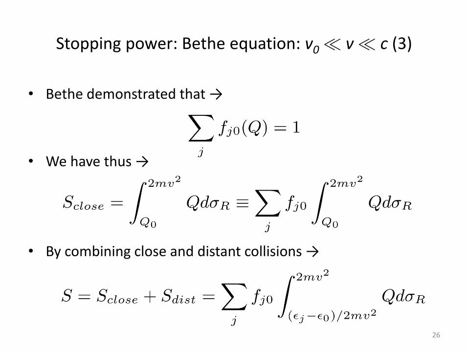
Stopping power: Bethe equation: v0 ¿ v ¿ c (3)
• Bethe demonstrated that →
• We have thus →
• By combining close and distant collisions →
26
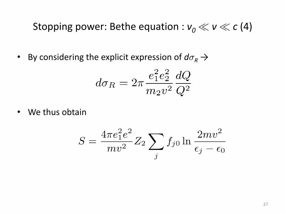
Stopping power: Bethe equation : v0 ¿ v ¿ c (4)
• By considering the explicit expression of d¾R →
• We thus obtain
27
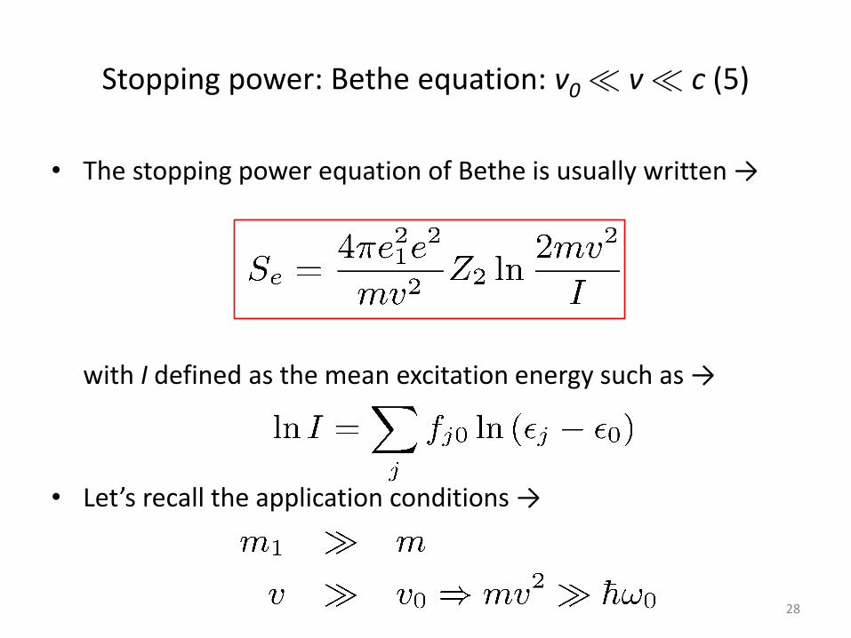
Stopping power: Bethe equation: v0 ¿ v ¿ c (5)
• The stopping power equation of Bethe is usually written →
with I defined as the mean excitation energy such as →
• Let’s recall the application conditions →
28
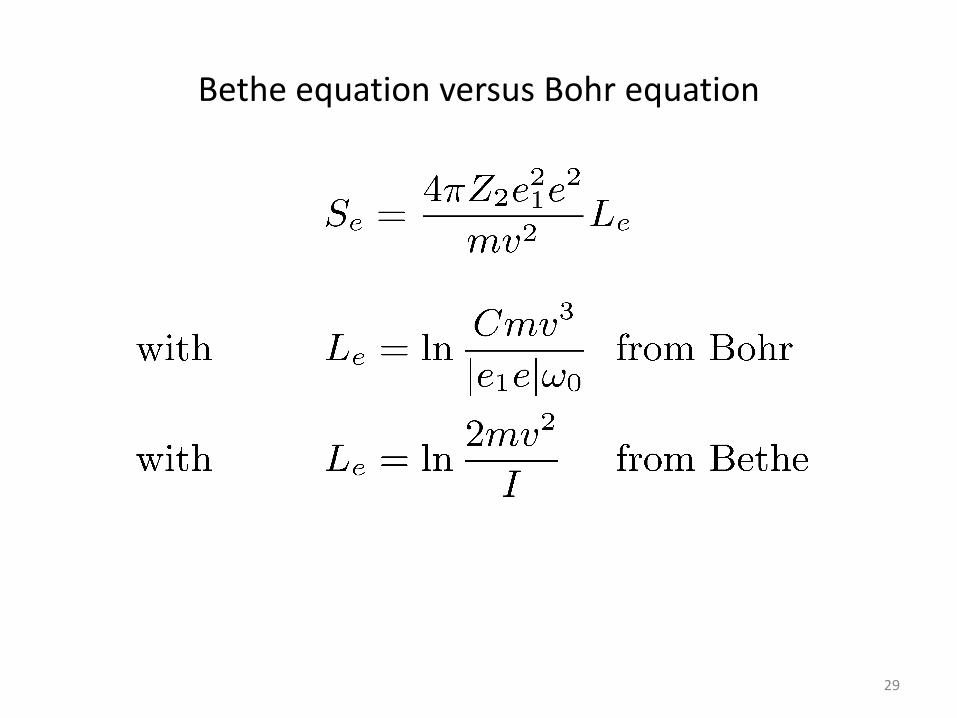
Bethe equation versus Bohr equation
29
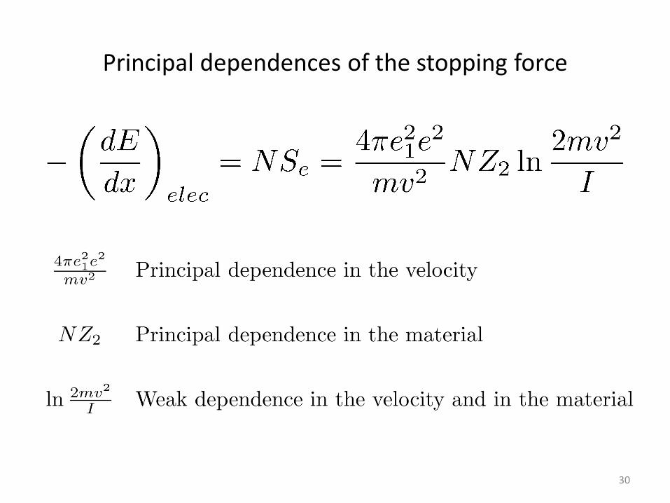
Principal dependences of the stopping force
30
Mean logarithmic excitation energy (1)
• The mean logarithmic excitation energy I only depends on the medium (not on the projectile)
• Difficult calculations → obtained from experiment
• I is in the logarithmic part of → not necessary to be known with precision
• I linearly varies (approximately) with Z → atomic model of Thomas-Fermi (atomic electrons = “gas”)
• The irregularities in the variation with Z are due to the shell structure of the atom
• Usually → evaluation of I with an empirical equation
31
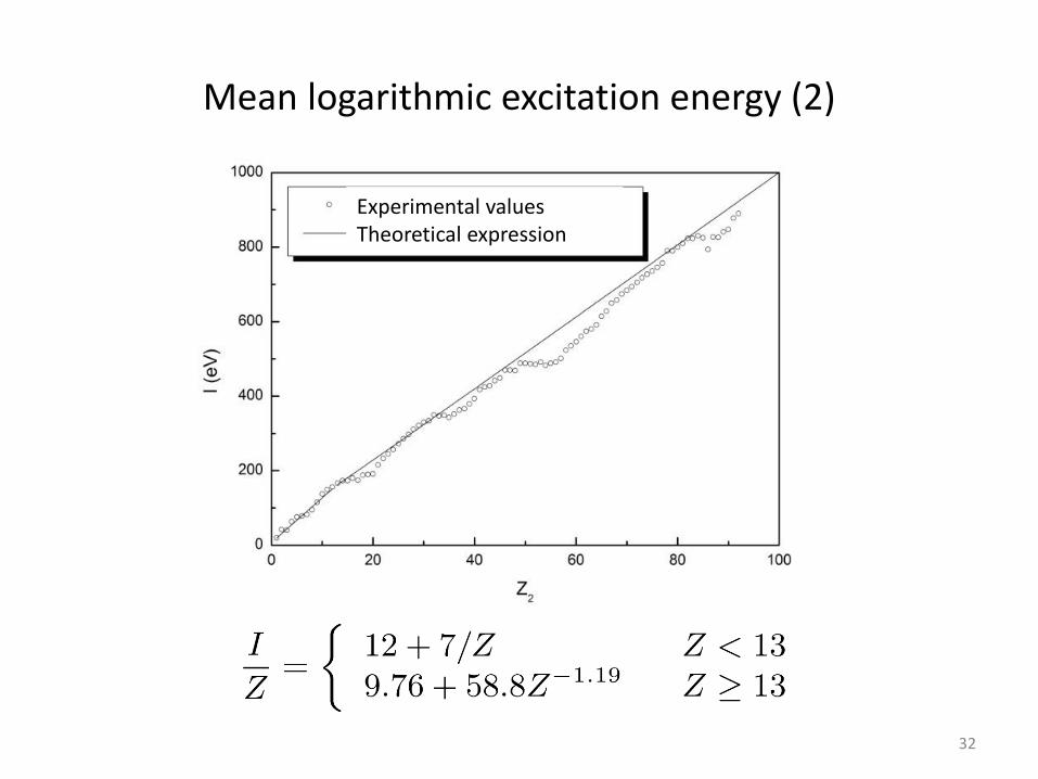
Mean logarithmic excitation energy (2)
32
Experimental values Theoretical expression
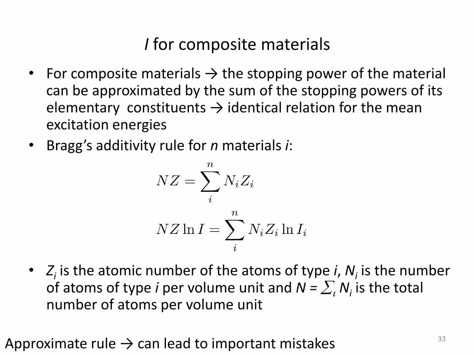
I for composite materials
• For composite materials → the stopping power of the material can be approximated by the sum of the stopping powers of its elementary constituents → identical relation for the mean excitation energies
• Bragg’s additivity rule for n materials i:
• Zi is the atomic number of the atoms of type i, Ni is the number of atoms of type i per volume unit and N = i Ni is the total number of atoms per volume unit
33 Approximate rule → can lead to important mistakes
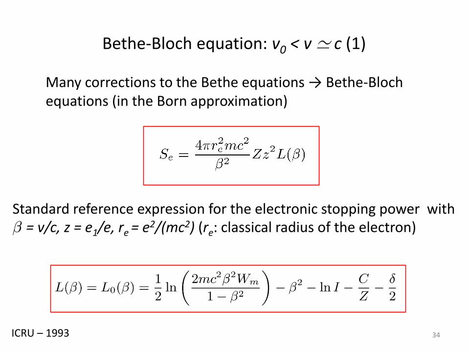
Bethe-Bloch equation: v0 < v ' c (1)
Many corrections to the Bethe equations → Bethe-Bloch equations (in the Born approximation)
34
Standard reference expression for the electronic stopping power with ¯ = v/c, z = e1/e, re = e2/(mc2) (re: classical radius of the electron)
ICRU – 1993
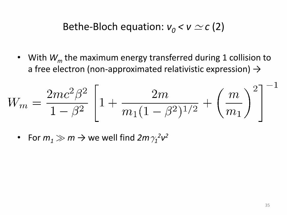
Bethe-Bloch equation: v0 < v ' c (2)
• With Wm the maximum energy transferred during 1 collision to a free electron (non-approximated relativistic expression) →
• For m1 À m → we well find 2m°12v2
35
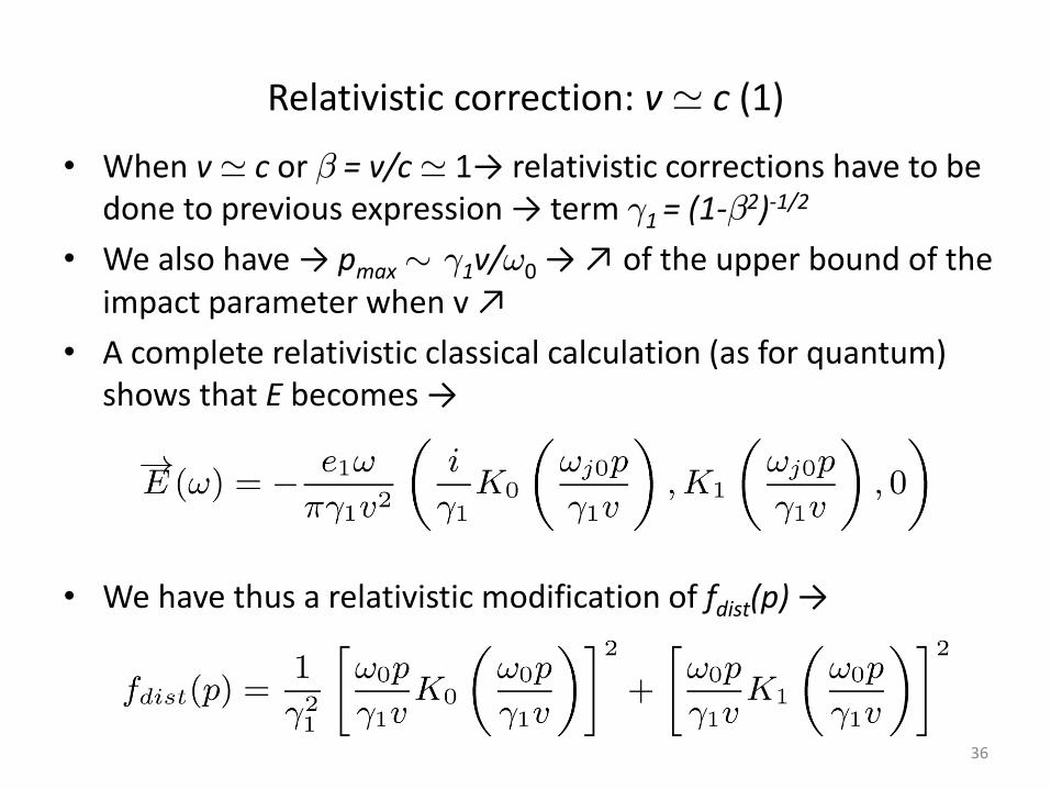
• When v ' c or ¯ = v/c ' 1→ relativistic corrections have to be done to previous expression → term °1 = (1-¯2)-1/2
• We also have → pmax » °1v/!0 → ↗ of the upper bound of the impact parameter when v ↗
• A complete relativistic classical calculation (as for quantum) shows that E becomes →
• We have thus a relativistic modification of fdist(p) →
Relativistic correction: v ' c (1)
36
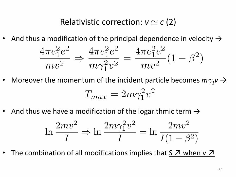
Relativistic correction: v ' c (2)
• And thus a modification of the principal dependence in velocity →
• Moreover the momentum of the incident particle becomes m°1v →
• And thus we have a modification of the logarithmic term →
• The combination of all modifications implies that S ↗ when v ↗
37
Density correction (1)
• Density correction → -±/2
• In the Bethe equation → interactions with isolated atoms → valid for low density gas
• In condensed matter (solid) → the interactions can get done with a large amount of atoms at once → we have to consider collective effects
• Model of Fermi (1940) → matter assimilated to a gas of oscillators submitted to the electric field of the particle
• Incident charged particle → polarization of matter → the electric field due to the charged particle disturb the atoms → they get a dipolar electric momentum → production of an electric field opposed to the field due to the charged particle → reduction of the electric field due to screening effect of the dipoles
38
Density correction (2)
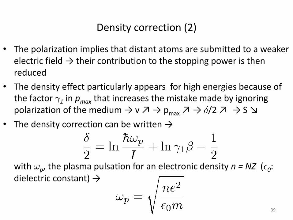
• The polarization implies that distant atoms are submitted to a weaker electric field → their contribution to the stopping power is then reduced
• The density effect particularly appears for high energies because of the factor °1 in pmax that increases the mistake made by ignoring polarization of the medium → v ↗ → pmax ↗ → ±/2 ↗ → S ↘
• The density correction can be written →
with !p, the plasma pulsation for an electronic density n = NZ (²0: dielectric constant) →
39
Density correction (3)
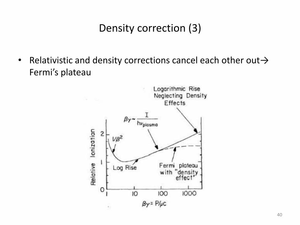
• Relativistic and density corrections cancel each other out→ Fermi’s plateau
40
Shell correction (1)
• Shell correction → -C/Z
• Bethe and Bohr equations supposed v À v0 (velocity of the atomic electrons) → the evaluation of I is based on this assumption → mean I value
• When it is not the case (v ↘) → it is necessary to explicitly calculate the ions-electrons interactions for each electron shell and for each electron binding energy
• When v ↘ → contribution to S of internal electrons (first K, then L, …) ↘
• “Mean” correction that reduces S (maximal correction = 6%) → = for all charged particles (including electrons) → only dependent on medium and velocity
41
Shell correction (2)
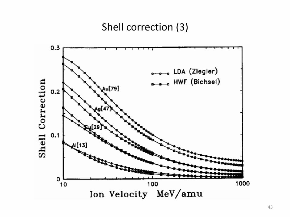
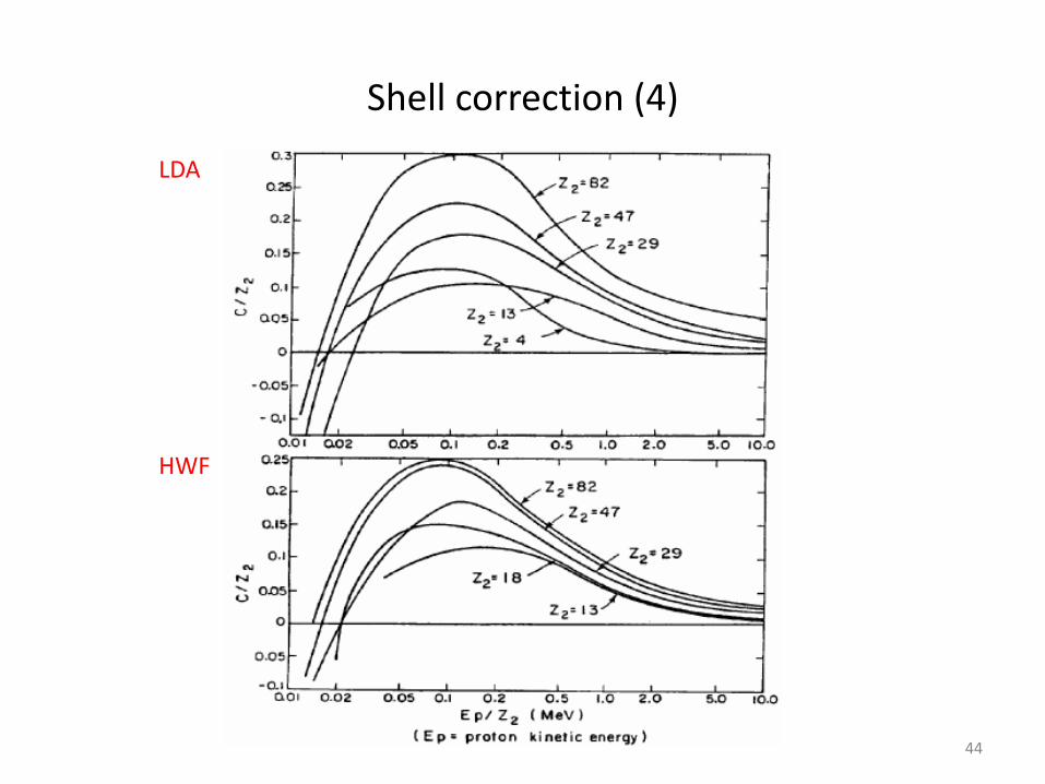
• 2 models to calculate C/Z →
1. The method of the hydrogenous wave functions (HWF: bound e- described by hydrogenous wave functions )
2. The method of the local density approximation (LDA: bound e- are a gas of e- with variable density)
42
Shell correction (3)
43
Shell correction (4)
44
LDA
HWF
Corrections beyond the first order Born approximation
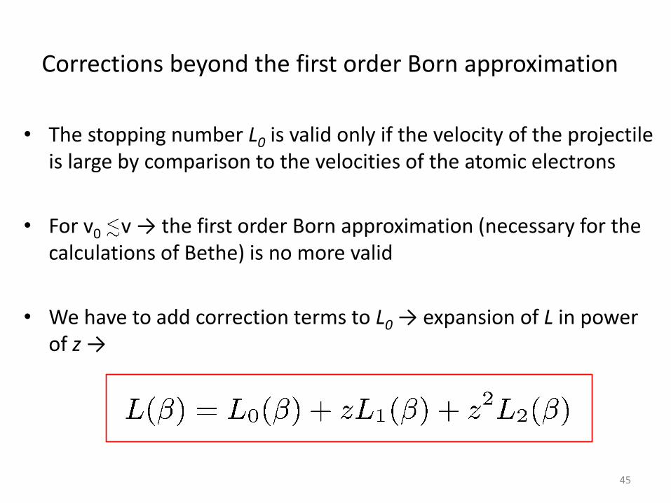
• The stopping number L0 is valid only if the velocity of the projectile is large by comparison to the velocities of the atomic electrons
• For v0 v → the first order Born approximation (necessary for the calculations of Bethe) is no more valid
• We have to add correction terms to L0 → expansion of L in power of z →
45
Barkas-Andersen correction
• Barkas-Andersen correction → zL1(¯)
• The Barkas-Andersen correction is proportional to an odd power in z (charge of the projectile) → S for negative particles is slightly weaker than for positive particles → S≠ between particles and corresponding antiparticles
• A positive charge attracts the e- → the interactions ↗ → S ↗
• A negative charge repulses the e- → the interactions ↘ → S ↘
46
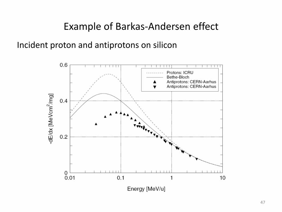
Example of Barkas-Andersen effect
Incident proton and antiprotons on silicon
47
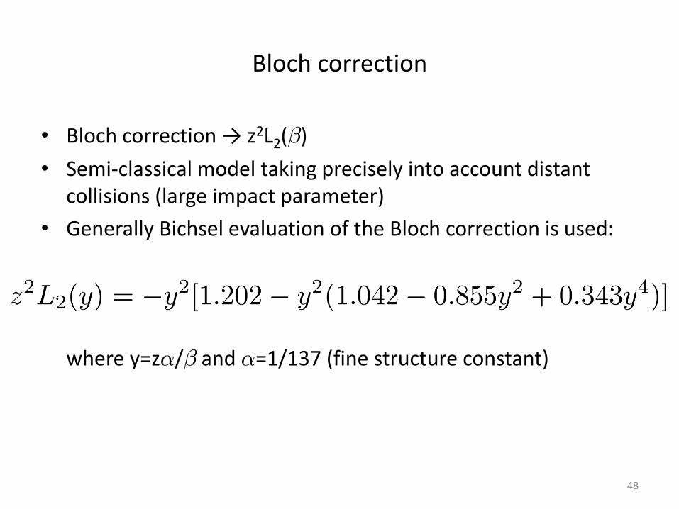
Bloch correction
• Bloch correction → z2L2(¯)
• Semi-classical model taking precisely into account distant collisions (large impact parameter)
• Generally Bichsel evaluation of the Bloch correction is used:
where y=z®/¯ and ®=1/137 (fine structure constant)
48
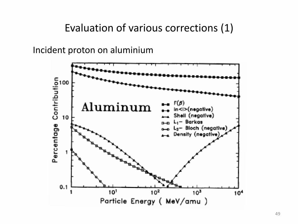
Evaluation of various corrections (1)
49
Incident proton on aluminium
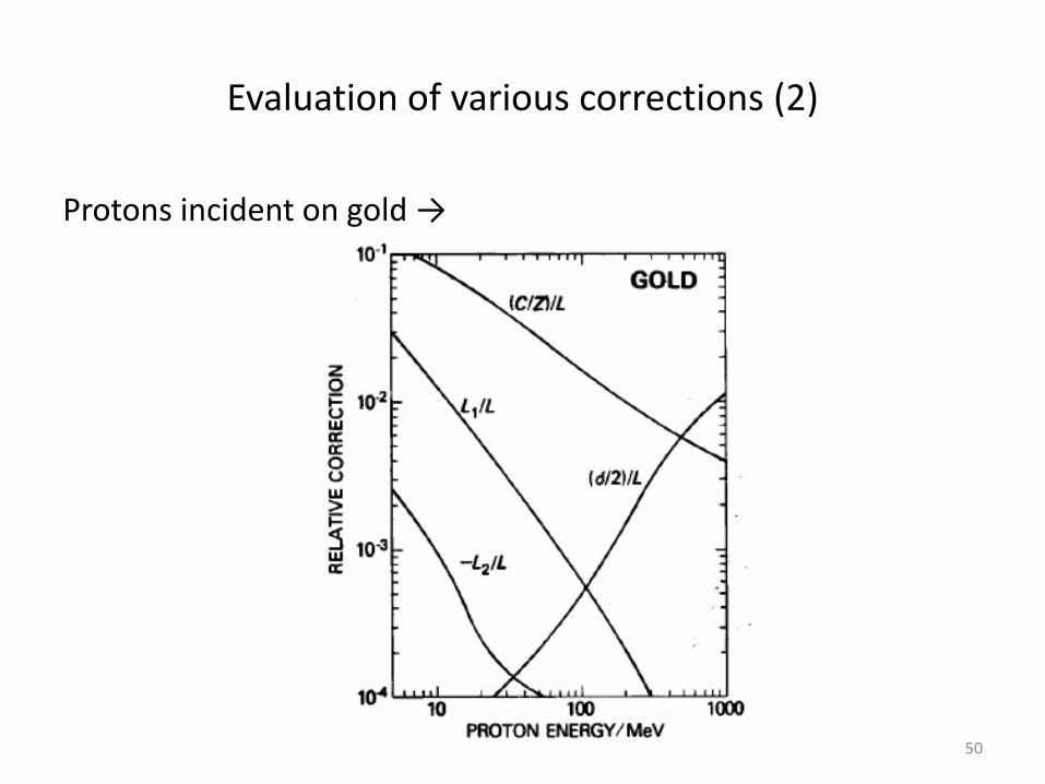
Evaluation of various corrections (2)
Protons incident on gold →
50
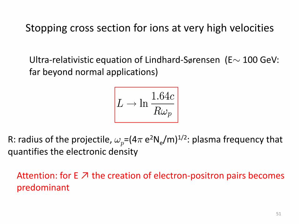
Stopping cross section for ions at very high velocities
Ultra-relativistic equation of Lindhard-Sørensen (E» 100 GeV: far beyond normal applications)
51
R: radius of the projectile, !p=(4¼ e2Ne/m)1/2: plasma frequency that quantifies the electronic density Attention: for E ↗ the creation of electron-positron pairs becomes predominant
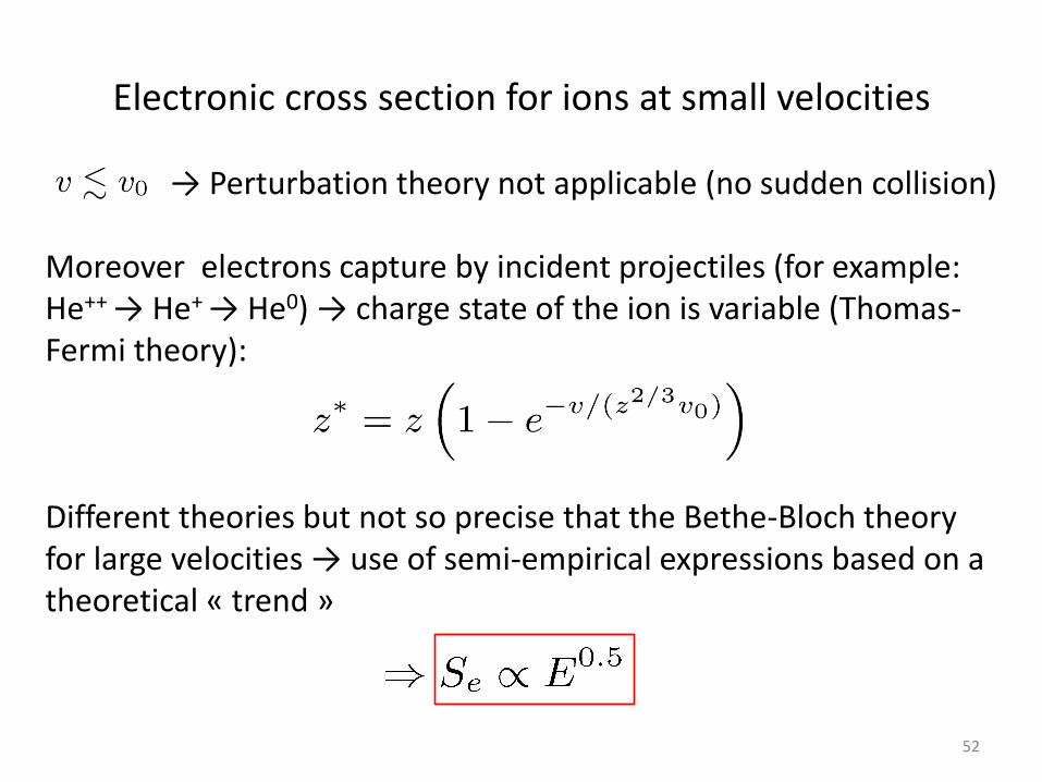
→ Perturbation theory not applicable (no sudden collision) Moreover electrons capture by incident projectiles (for example: He++ → He+ → He0) → charge state of the ion is variable (Thomas-Fermi theory): Different theories but not so precise that the Bethe-Bloch theory for large velocities → use of semi-empirical expressions based on a theoretical « trend »
Electronic cross section for ions at small velocities
52
Nuclear cross section for ions at small velocities (1)
• Chapter 1 → Nuclear collisions for incidents ions are rare → small contribution to the total stopping power
• Only for incident ions with small velocity → even in that case their contribution is small
• However → They can have effects a posteriori → radiative damages
53
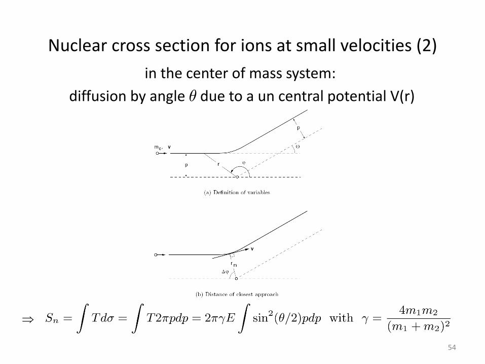
Nuclear cross section for ions at small velocities (2)
54
in the center of mass system:
diffusion by angle µ due to a un central potential V(r)
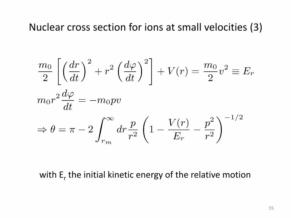
Nuclear cross section for ions at small velocities (3)
55
with Er the initial kinetic energy of the relative motion
Nuclear cross section for ions at small velocities (4)
56
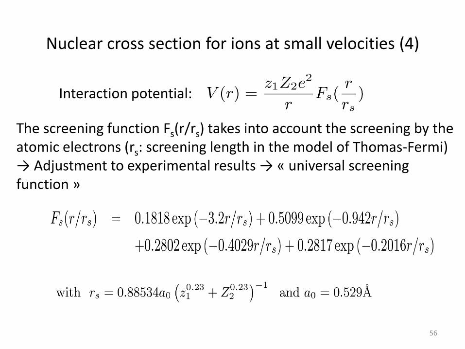
Interaction potential:
The screening function Fs(r/rs) takes into account the screening by the atomic electrons (rs: screening length in the model of Thomas-Fermi) → Adjustment to experimental results → « universal screening function »
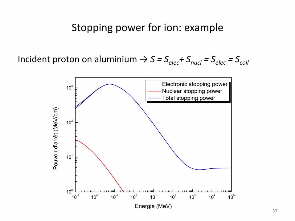
Stopping power for ion: example
Incident proton on aluminium → S = Selec+ Snucl ≈ Selec = Scoll
57
Electronic mass stopping power (1)
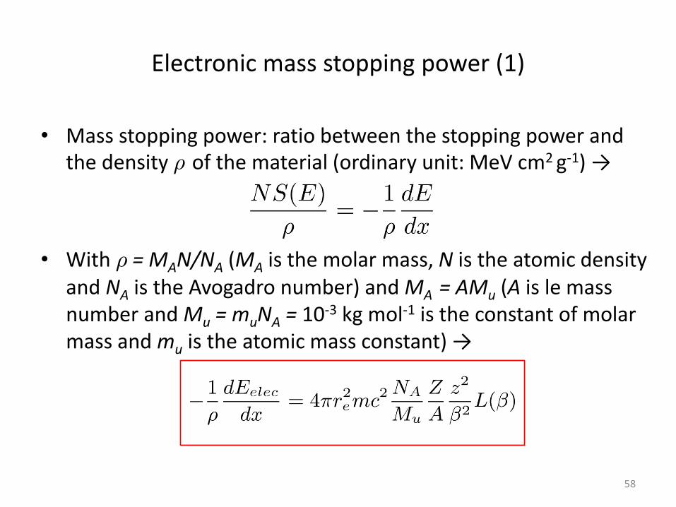
• Mass stopping power: ratio between the stopping power and the density ½ of the material (ordinary unit: MeV cm2 g-1) →
• With ½ = MAN/NA (MA is the molar mass, N is the atomic density and NA is the Avogadro number) and MA = AMu (A is le mass number and Mu = muNA = 10-3 kg mol-1 is the constant of molar mass and mu is the atomic mass constant) →
58
Electronic mass stopping power (2)
The electronic mass stopping power is the product of 4 factors:
1. The constant factor 4¼re2mc2NA/Mu = 0.307 MeV cm2 g-1 →
order of magnitude for the electronic mass stopping power
2. The factor Z/A that is included between 0.4 et 0.5 for all stable isotopes (except hydrogen) → weak dependency into the medium
3. The factor ¯-2 → monotonic decreasing function in ion velocity that tends to 1 for large energies → explain the decrease of the stopping power as a function of the energy
4. The stopping number L(¯) → for L(¯) = L0(¯) → monotonic increasing function (slow) in the velocity and in Z (via I: -ln I)
59
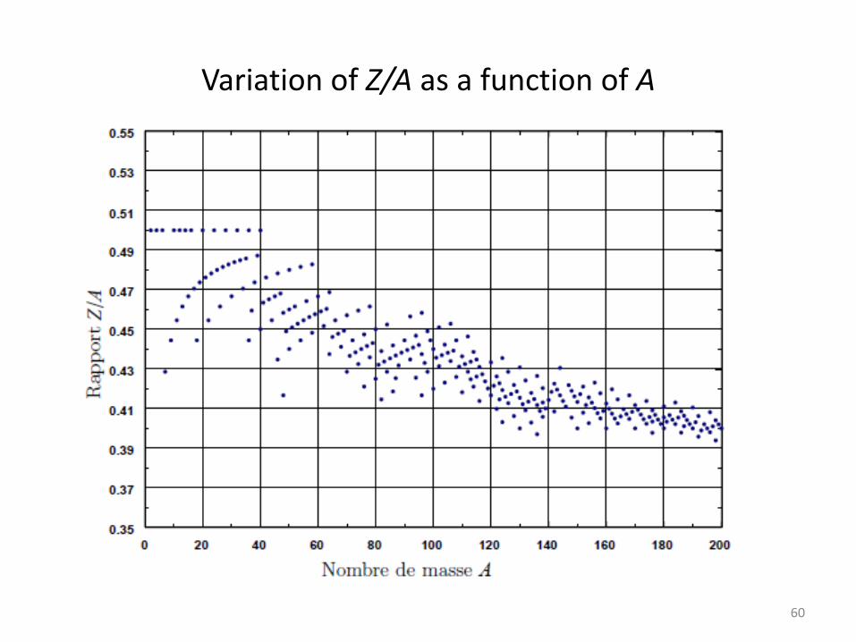
Variation of Z/A as a function of A
60
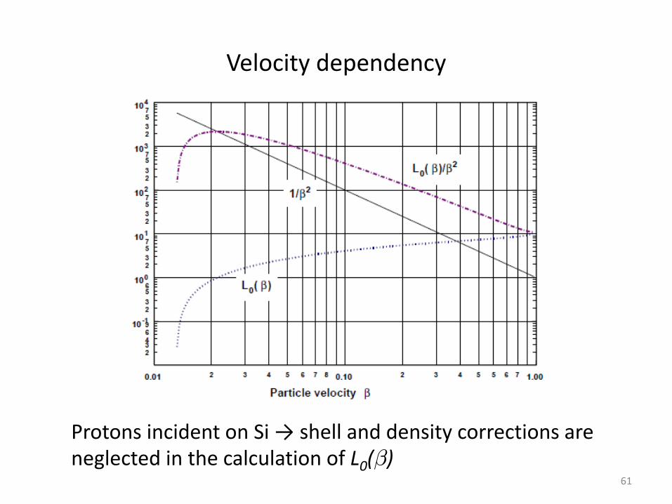
Velocity dependency
Protons incident on Si → shell and density corrections are neglected in the calculation of L0(¯)
61
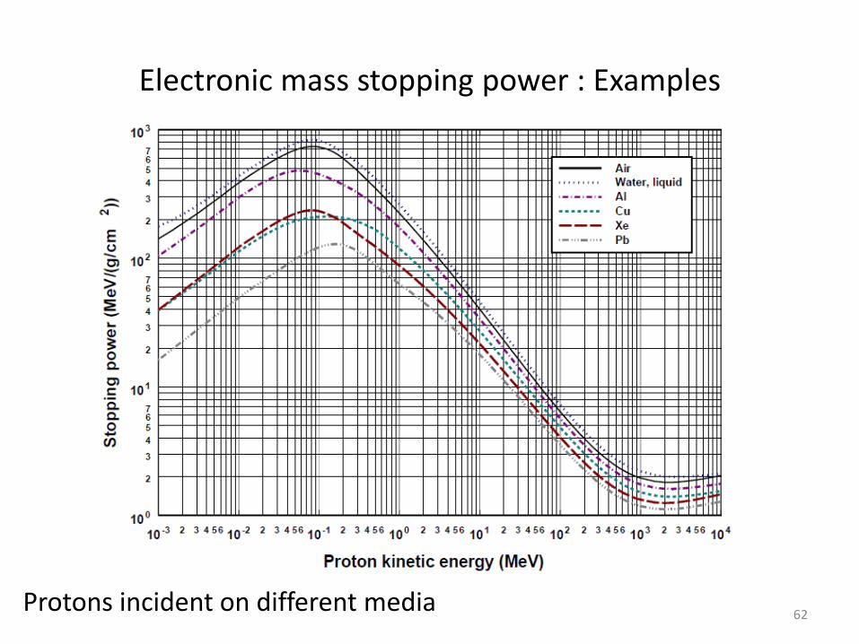
Electronic mass stopping power : Examples
Protons incident on different media 62
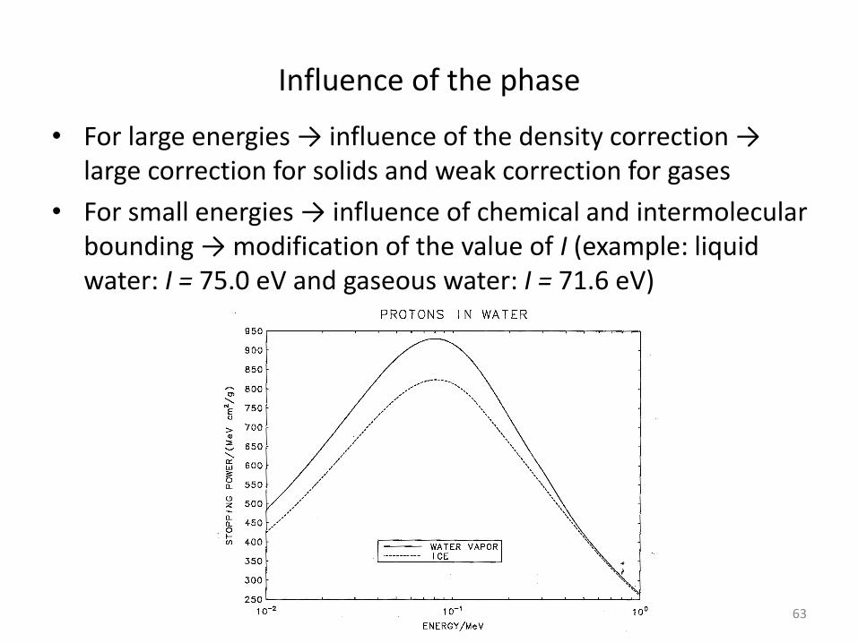
Influence of the phase
• For large energies → influence of the density correction → large correction for solids and weak correction for gases
• For small energies → influence of chemical and intermolecular bounding → modification of the value of I (example: liquid water: I = 75.0 eV and gaseous water: I = 71.6 eV)
63
Range of charged particles (1)
• Charged particles lose their energy in matter → they travel a certain distance in matter → this distance is variable because of aleatory energy losses and deviations (straggling) → different ranges have to be defined: – The range R of a charged particle of energy E in a medium is the mean value
h l i of the length l of its trajectory as it slows down to rest (we do not take into account thermal motion)
– The projected range Rp of a charged particle of energy E in a medium is the mean value of its penetration depth h d i along the initial direction of the particle
• Rp < R due to the sinuous character of trajectories → definition of the detour factor = RP/RCSDA < 1
64
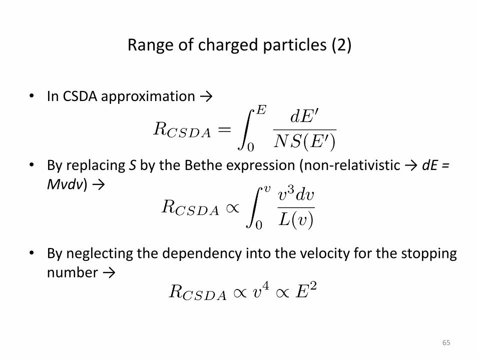
Range of charged particles (2)
• In CSDA approximation →
• By replacing S by the Bethe expression (non-relativistic → dE = Mvdv) →
• By neglecting the dependency into the velocity for the stopping number →
65
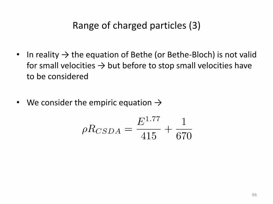
Range of charged particles (3)
• In reality → the equation of Bethe (or Bethe-Bloch) is not valid for small velocities → but before to stop small velocities have to be considered
• We consider the empiric equation →
66
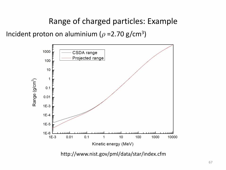
Range of charged particles: Example
67
Incident proton on aluminium (½ =2.70 g/cm3)
http://www.nist.gov/pml/data/star/index.cfm
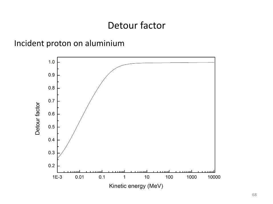
Detour factor
68
Incident proton on aluminium
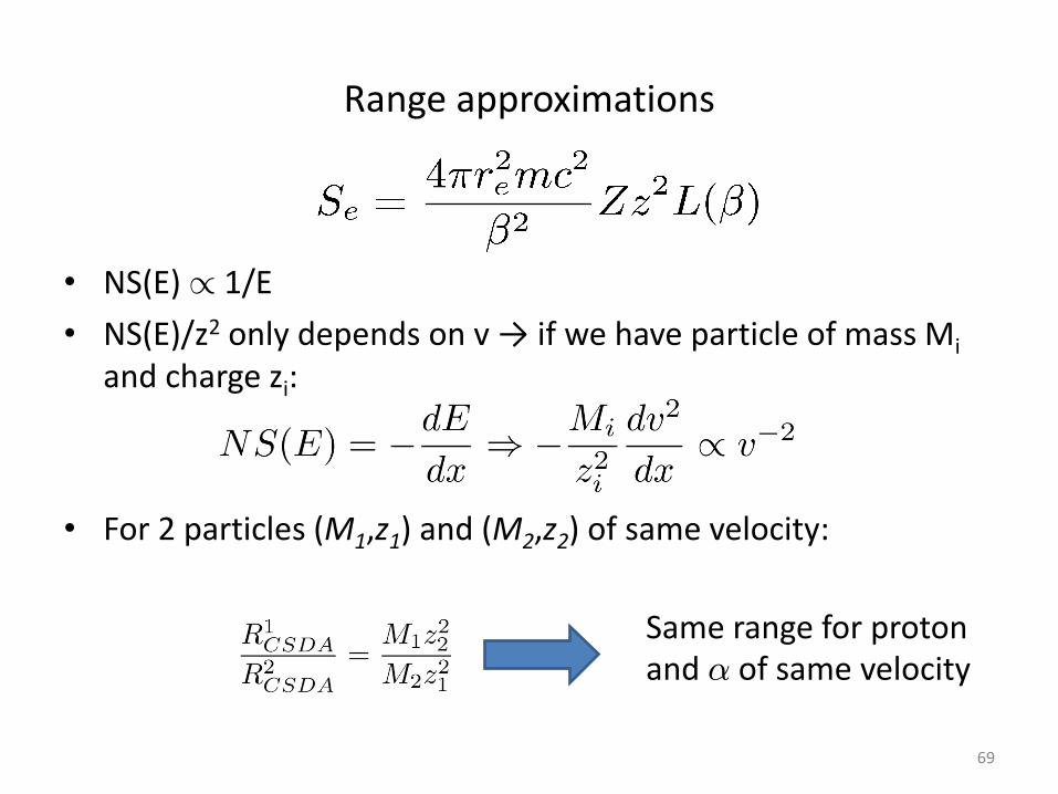
Range approximations
• NS(E) / 1/E
• NS(E)/z2 only depends on v → if we have particle of mass Mi and charge zi:
• For 2 particles (M1,z1) and (M2,z2) of same velocity:
69
Same range for proton and ® of same velocity
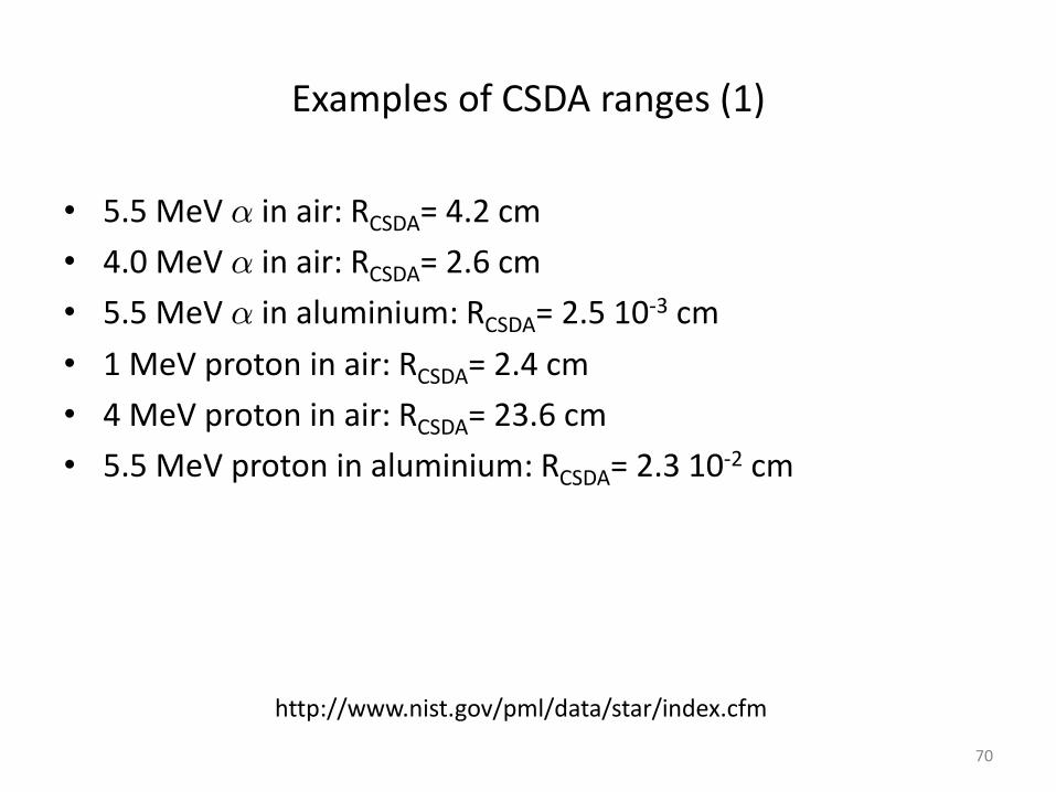
Examples of CSDA ranges (1)
• 5.5 MeV ® in air: RCSDA= 4.2 cm
• 4.0 MeV ® in air: RCSDA= 2.6 cm
• 5.5 MeV ® in aluminium: RCSDA= 2.5 10-3 cm
• 1 MeV proton in air: RCSDA= 2.4 cm
• 4 MeV proton in air: RCSDA= 23.6 cm
• 5.5 MeV proton in aluminium: RCSDA= 2.3 10-2 cm
70
http://www.nist.gov/pml/data/star/index.cfm
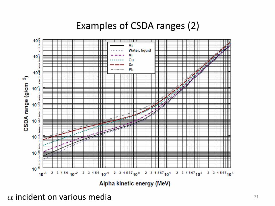
Examples of CSDA ranges (2)
® incident on various media
71
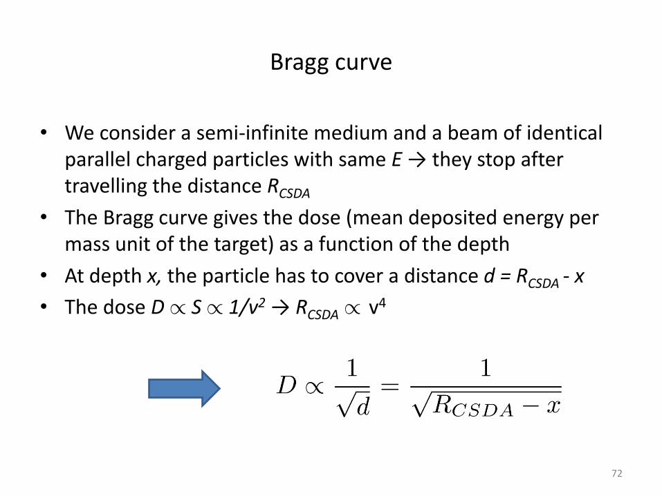
Bragg curve
• We consider a semi-infinite medium and a beam of identical parallel charged particles with same E → they stop after travelling the distance RCSDA
• The Bragg curve gives the dose (mean deposited energy per mass unit of the target) as a function of the depth
• At depth x, the particle has to cover a distance d = RCSDA - x
• The dose D / S / 1/v2 → RCSDA / v4
72
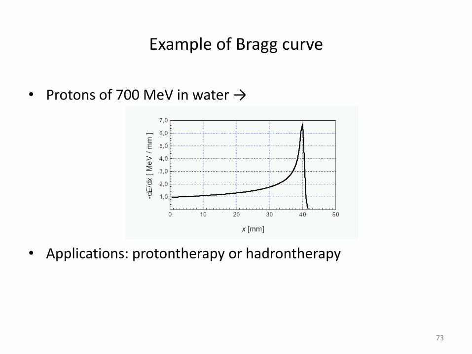
Example of Bragg curve
• Protons of 700 MeV in water →
• Applications: protontherapy or hadrontherapy
73
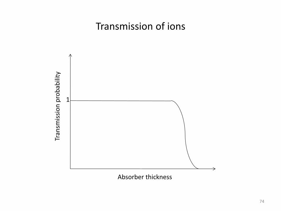
Transmission of ions
74
Absorber thickness
Tran
smis
sio
n p
rob
abili
ty
1
Strong nuclear interactions
• If ion comes very close to target nucleus → strong nuclear interaction becomes possible → the target nucleus will be broken up
• One particular case: the collision of a high-energy proton with a very heavy nucleus with thus more neutrons than protons (lead: 82 protons and ≈125 neutrons) → the fragments will quickly expel their excess neutrons → production of a large number of secondary neutrons (proton of 1 GeV → on average 25 neutrons in lead)
• This process of neutrons production is called spallation → efficient way to produce neutrons
• All fragments interact with matter
75